IEEE TRANSACTIONS ON MAGNETICS, VOL. 49, NO. 5, MAY 2013 1833
Non-Conforming Sliding Interfaces for Relative Motion in 3D FiniteElement Analysis of Electrical Machines by Magnetic Scalar
Potential Formulation Without CutsStefan Boehmer , Enno Lange , and Kay Hameyer
Institute of Electrical Machines, RWTH Aachen University, Aachen, D-52062 GermanyCST-Computer Simulation Technology AG, Darmstadt, D-64289 Germany
This paper discusses non-conforming sliding interfaces for motion in combination with a magnetic scalar potential formulation. La-grange multiplier are used to implement the relative motion of stator and rotor. The utilization of the specific Lagrange multiplierapproach implies the application of a magnetic scalar potential formulation in 3D Finite Element (FE) modeling of electrical machinesbecause up to the present a canonical definition of biorthogonal basis functions for the magnetic vector potential is not available.Classical magnetic scalar potential formulations require the definition of cuts to make the potential single-valued. The presented ap-
proach uses a decomposition of the magnetic field into a scalar potential and loop fields defined on the whole domain to avoid the explicitdefinition of cuts.
Index Terms—Dual formulation, electrical machines, finite element methods, sliding interfaces.
I. INTRODUCTION
N OWADAYS several approaches for handling relative mo-tion of stator and rotor in FE analysis of electrical ma-
chines are available [1], [2]. Static, transient and particularlyfield coupling simulations of electrical machines require theflexible displacement of the rotor by an arbitrary angle in ro-tating machines or a distance in translational electric machines.In 2D FE modeling the Moving-Band method can be employedwhere an annulus-shaped band in the airgap between rotor andstator is remeshed in every time step [3]. In 3D FEmodeling thisapproach is not feasible because it would require a full meshgenerator whereas remeshing is done by a simple mapping in2D. Thus, the Lockstep method [1] is usually applied in 3Dwhich is based on a regular discretization of the rotor and thestator surfaces. The major disadvantage of this method is thelack of arbitrary displacement because step size is fixed by thediscretization. As a consequence, a smooth movement leads to asignificant increase in the number of elements resulting in an in-crease of computing time which is highly undesirable. Lagrangemultiplier approaches seek to overcome the disadvantages beingapplicable to 2D as well as 3D problems [4], [5].
II. MOTION BY LAGRANGE MULTIPLIER
The Lagrange multiplier method ensures the continuity ofthe fields across the non-conforming interface between thestationary and moving FE discretizations of the stator androtor of the electrical machine. As a consequence an arbitrarydisplacement without restrictions in time or space discretizationis possible. In general, the application of Lagrange multipliermethods yields a saddle point problem, which cannot besolved by standard Krylov-subspace algorithms. In order topreserve the numerical properties of a conforming approach,the FE-space of the discrete Lagrange multiplier is spanned by
Manuscript received October 31, 2012; revised January 12, 2013; acceptedJanuary 13, 2013. Date of current version May 07, 2013. Corresponding author:S. Boehmer (e-mail: [email protected]).Color versions of one or more of the figures in this paper are available online
at http://ieeexplore.ieee.org.Digital Object Identifier 10.1109/TMAG.2013.2242051
basis functions fulfilling the biorthogonality condition as de-scribed in [4] and applied to electromagnetic field computationin [2] and [6]. Thereby, the resulting symmetric positive definitesystem can be solved by Krylov-subspace algorithms. Previousstudies have indicated that it is not feasible to construct suchbiorthogonal basis function in 3D for the magnetic vector po-tential formulation in a canonical way but for magnetic scalarpotential formulation [2].In the presented paper the authors hence utilize the magnetic
scalar potential formulation shown in [7] and simplify the algo-rithm to compute the source fields on basis of spanning trees.Furthermore, this algorithm is extended to overcome possibletermination issues. The resulting method is combined with theLagrange multiplier approach presented by the authors in [2]and is applied to an exemplary electrical machine.
III. TOPOLOGICAL STRUCTURE
In the classical formulation the field is computed in theconducting region only whereas is computed in the whole do-main ([8], [9]). This approach requires the definition of cuts inthe non-conducting domain for multiple connected regions be-cause otherwise may become multi-valued. In order to avoidthese cuts the approach in this paper consists in decomposingthe magnetic field appropriately. The theoretical backgroundhas been presented in [7] and is recapitulated as far as necessary.Let be a connected mesh, the non-conducting
domain, the domain of all conductors and itsboundary as shown in Fig. 1. Furthermore, let be the setof differential forms of degree which are defined on the do-main . In the non-conducting domain one has to solve
and with and :
(1)
While can be satisfied by introduction of the magneticvector potential with , the situation is more com-plicated for . The Poincaré lemma states that canbe represented by a continuous gradient field in
1834 IEEE TRANSACTIONS ON MAGNETICS, VOL. 49, NO. 5, MAY 2013
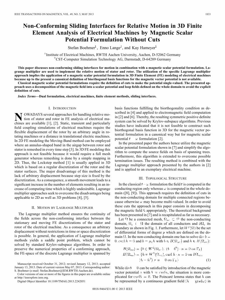
Fig. 1. Volumes and surfaces in the 3D domain [7].
a contractible domain like a ball or a tetrahedron. If the domaincontains holes and thus is not contractible, the topological struc-ture of the functional space has to be considered. Let
be the set of all gradients and the set of allcurl-free fields on . Following De Rham’s theorem the quo-tient vector space is of finitedimension and equals the number of holes in , respectivelythe number of independent loops formed by the conduc-tors, also called Betti number . The first cohomology group
represents the set of curl-free 1-forms which cannotbe expressed as a gradient of a 0-form.The magnetic field in can then be expressed by
(2)
where is the current in conductor loop which is imposedin an independent section of the conductor as seen in Fig. 1and is a continuous scalar potential without cutsdefined on
(3)
The loop fields form a basis of the first coho-mology group and are computed for every singleby imposing a unity current in and zero current in all other
. Instead of a direct computation of , whichis in general a task of high complexity, we utilize the duality be-tween cohomology and homology groups. The first homologygroup is defined as the set ofall closed curves in which are not the boundary of any sur-face in . By De Rham’s theorem the first homology group isisomorph to the first cohomology group .The construction of the loop fields can hence be achieved by
three single steps:1) Generate a basis for the first homology groupwhich is done by the definition of the surfaces .
2) Build a spanning tree on corresponding to .3) For each construct a basis of the first cohomology group
which forms the according loop field.
IV. CONSTRAINED SPANNING TREE
The presented approach of using spanning trees is a modifiedand extended version of [7] which is based on [10]. An (edge)spanning tree of a mesh is a subset of edges which does notcontain any cycle and visits every node of the mesh.To construct a constrained spanning tree, it is necessary to
build a spanning tree on which is also a spanning tree onall constrained volumes and surfaces. Therefore, the followingconstraints have to be considered:
• curl on• curl on• on S• on•
The algorithm to construct the spanning tree, which is de-scribed later in this section, works by iteratively appendingedges to the tree which do not close a cycle and hence pre-serve the spanning tree property. To ensure that the spanningtree is also valid on the constrained volumes and surfaces,edges corresponding to these sets have to be put into the treebefore other ones. This is ensured by assigning a priority toevery edge in the mesh. Let us denote the set of volumes by
and the set of the constrained surfacesby .The set of edges corresponding to the volume , or the surfaceare denoted by and respectively and the priority
of edge is denoted by . In contrast to the algorithmpresented in [7] a simpler algorithm to compute the priority forall edges is proposed:
1) For each edge in (all edges):•
2) For each volume :• For each edge in :
3) For each surface :• For each edge in :
This algorithm ensures that a higher priority is assigned to anedge which is contained in more volumes and surfaces thanan edge which is contained in fewer entities.Afterwards, the constrained spanning tree can be constructed
by the following straightforward algorithm which appends iter-atively edges to the set representing the spanning tree. Theset contains all the nodes visited by the spanning tree:
1)2) Pick one arbitrary initial node and append it to3) Append all edges associated with to4) While :• Pick and remove one edge with highestpriority from
• If end node not in :— Append to—Append to— Insert all edges associated with into
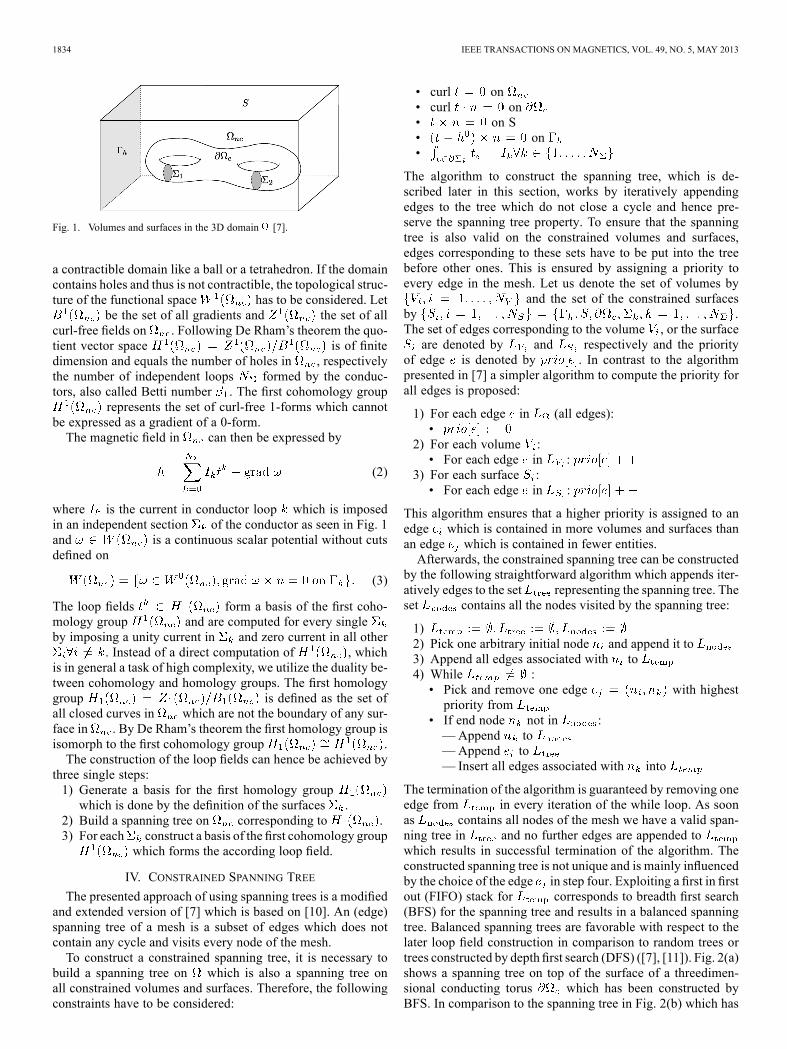
The termination of the algorithm is guaranteed by removing oneedge from in every iteration of the while loop. As soonas contains all nodes of the mesh we have a valid span-ning tree in and no further edges are appended towhich results in successful termination of the algorithm. Theconstructed spanning tree is not unique and is mainly influencedby the choice of the edge in step four. Exploiting a first in firstout (FIFO) stack for corresponds to breadth first search(BFS) for the spanning tree and results in a balanced spanningtree. Balanced spanning trees are favorable with respect to thelater loop field construction in comparison to random trees ortrees constructed by depth first search (DFS) ([7], [11]). Fig. 2(a)shows a spanning tree on top of the surface of a threedimen-sional conducting torus which has been constructed byBFS. In comparison to the spanning tree in Fig. 2(b) which has
BOEHMER et al.: NON-CONFORMING SLIDING INTERFACES FOR RELATIVE MOTION IN 3D FINITE ELEMENT ANALYSIS 1835
Fig. 2. Spanning tree on the top surface of a torus. (a) breadth first search,(b) depth first search.
Fig. 3. Spanning tree on the surface of a torus with .
been constructed by DFS, one can observe that BFS results inmuch more nodes with branching edges.
V. LOOP FIELDS
After the construction of the spanning tree on the loopfields can be build which have to fulfill the condition curlon the non-conducting domain using edge-basedWhitneyelements. This is done iteratively for every by imposing aunity current in and zero current in all other .By construction of the spanning tree there is exactly one edgefor every set which is not contained in the tree. Thisis illustrated in Fig. 3 where is highlighted by exposing itsnodes by spheres and all the tree edges in being drawnby bold edges. It can be seen, that the top left edge ofis the only edge which is not contained in the spanning tree.Therefore, it is possible to impose unity current by assigning aunity value to the edge with . Tocompute the desired loop fields , it is necessary to satisfy thecurl condition for all faces in the non-conducting region :
(4)
where denotes all faces of elements in . Equation(4) can be transformed to a linear system of equations with un-known for every edge and one equation for every face
. This system of equation does not have full rank, thereis an infinite number of possible loop fields , but the kernelof the system of equations can be eliminated by fixing all edgevalues corresponding to spanning tree edges [12].This results in a unique solution of the system of equations andthus to a unique loop field .Instead of utilizing an equation solver, the algorithm to com-
pute the loop field for works by backsubstitution as fol-lows (cf. [7]):1) Set all values of tree edges to zero:2) For each in :• Set for
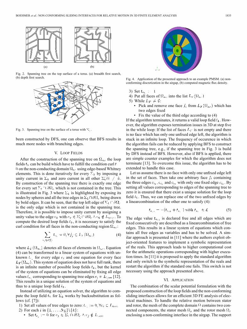
Fig. 4. Application of the presented approach to an example PMSM. (a) non-conforming discretization in the airgap, (b) computed magnetic flux density.
3) Set4) Put all faces of into the list5) While :• Pick and remove one face from which hastwo edges fixed
• Fix the value of the third edge according to (4)If the algorithm terminates, it returns a valid loop field . How-ever, the algorithm exposes termination issues in 3D at step fivein the while loop: If the list of faces is not empty and thereis no face which has only one unfixed edge left, the algorithm isstuck in an infinite loop. The frequency of occurence in whichthe algorithm fails can be reduced by applying BFS to constructthe spanning tree, e.g., if the spanning tree in Fig. 3 is buildby DFS instead of BFS. However, also if BFS is applied, thereare simple counter examples for which the algorithm does notterminate [13]. To overcome this issue, the algorithm has to beextended to handle this case.Let us assume there is no face with only one unfixed edge left
in the set of faces. Then take one arbitrary face containingthe three edges and with only one fixed edge . Bysetting all values corresponding to edges of the spanning tree tozero it is ensured that there exist a unique solution for the loopfield . Thus, we can replace one of the two unfixed edges bya linearcombination of the other one to satisfy (4):
(5)
The edge value is declared free and all edges which arefixed consecutively are described as a linearcombination of freeedges. This results in a linear system of equations which con-tains all free edges as variables and has to be solved. A sim-ilar approach is presented in [11] where the authors exploit ob-ject-oriented features to implement a symbolic representationof the reals. This approach leads to higher computational costfor the arithmetic operations corresponding with higher execu-tion times. In [11] it is proposed to apply the standard algorithmand only switch to the symbolic representation of the reals andrestart the algorithm if the standard one fails. This switch is notnecessary using the approach presented above.
VI. APPLICATION
The combination of the scalar potential formulation with theproposed construction of the loop fields and the non-conformingsliding interfaces allows for an efficient 3D FE analysis of elec-trical machines. To handle the relative motion between statorand rotor, the mesh of the complete domain contains two con-nected components, the stator mesh and the rotor meshenclosing a non-conforming interface in the airgap. The support
1836 IEEE TRANSACTIONS ON MAGNETICS, VOL. 49, NO. 5, MAY 2013
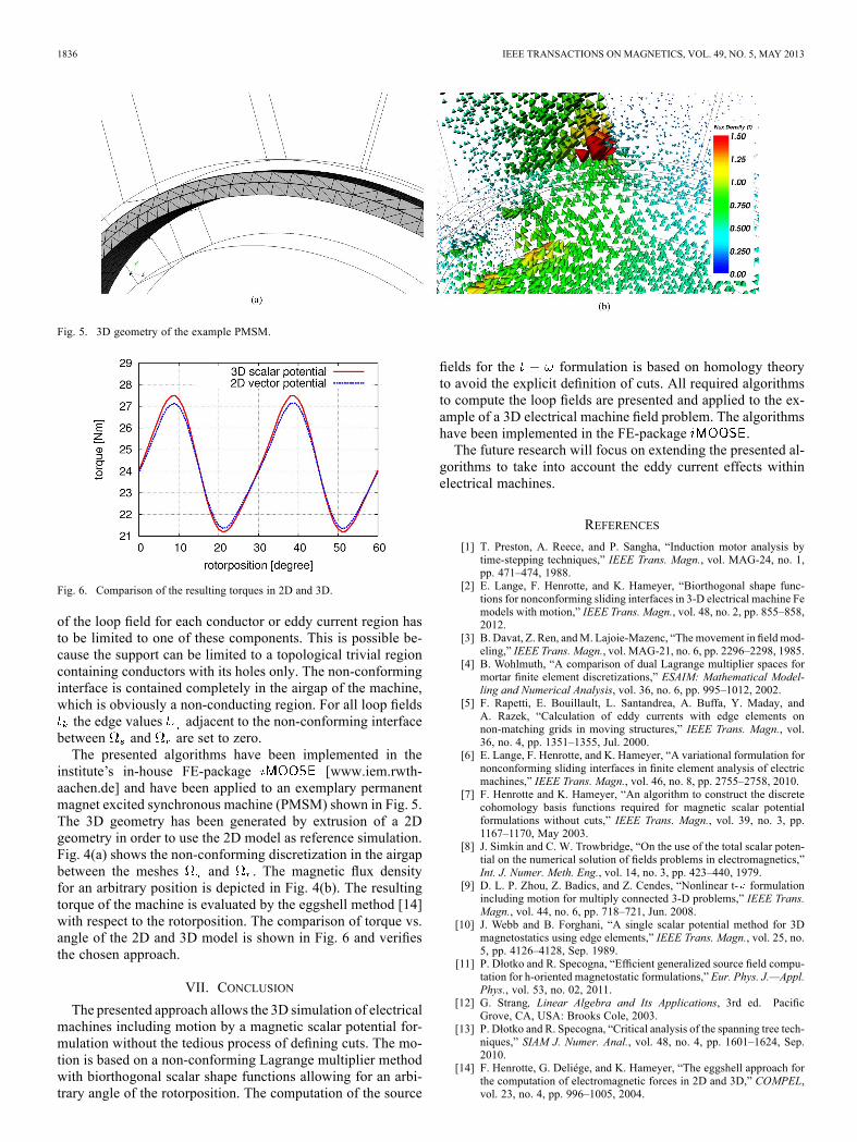
Fig. 5. 3D geometry of the example PMSM.
Fig. 6. Comparison of the resulting torques in 2D and 3D.
of the loop field for each conductor or eddy current region hasto be limited to one of these components. This is possible be-cause the support can be limited to a topological trivial regioncontaining conductors with its holes only. The non-conforminginterface is contained completely in the airgap of the machine,which is obviously a non-conducting region. For all loop fieldsthe edge values adjacent to the non-conforming interface
between and are set to zero.The presented algorithms have been implemented in the
institute’s in-house FE-package [www.iem.rwth-aachen.de] and have been applied to an exemplary permanentmagnet excited synchronous machine (PMSM) shown in Fig. 5.The 3D geometry has been generated by extrusion of a 2Dgeometry in order to use the 2D model as reference simulation.Fig. 4(a) shows the non-conforming discretization in the airgapbetween the meshes and . The magnetic flux densityfor an arbitrary position is depicted in Fig. 4(b). The resultingtorque of the machine is evaluated by the eggshell method [14]with respect to the rotorposition. The comparison of torque vs.angle of the 2D and 3D model is shown in Fig. 6 and verifiesthe chosen approach.
VII. CONCLUSION
The presented approach allows the 3D simulation of electricalmachines including motion by a magnetic scalar potential for-mulation without the tedious process of defining cuts. The mo-tion is based on a non-conforming Lagrange multiplier methodwith biorthogonal scalar shape functions allowing for an arbi-trary angle of the rotorposition. The computation of the source
fields for the formulation is based on homology theoryto avoid the explicit definition of cuts. All required algorithmsto compute the loop fields are presented and applied to the ex-ample of a 3D electrical machine field problem. The algorithmshave been implemented in the FE-package .The future research will focus on extending the presented al-
gorithms to take into account the eddy current effects withinelectrical machines.
REFERENCES
[1] T. Preston, A. Reece, and P. Sangha, “Induction motor analysis bytime-stepping techniques,” IEEE Trans. Magn., vol. MAG-24, no. 1,pp. 471–474, 1988.
[2] E. Lange, F. Henrotte, and K. Hameyer, “Biorthogonal shape func-tions for nonconforming sliding interfaces in 3-D electrical machine Femodels with motion,” IEEE Trans. Magn., vol. 48, no. 2, pp. 855–858,2012.
[3] B. Davat, Z. Ren, andM. Lajoie-Mazenc, “Themovement in field mod-eling,” IEEE Trans. Magn., vol. MAG-21, no. 6, pp. 2296–2298, 1985.
[4] B. Wohlmuth, “A comparison of dual Lagrange multiplier spaces formortar finite element discretizations,” ESAIM: Mathematical Model-ling and Numerical Analysis, vol. 36, no. 6, pp. 995–1012, 2002.
[5] F. Rapetti, E. Bouillault, L. Santandrea, A. Buffa, Y. Maday, andA. Razek, “Calculation of eddy currents with edge elements onnon-matching grids in moving structures,” IEEE Trans. Magn., vol.36, no. 4, pp. 1351–1355, Jul. 2000.
[6] E. Lange, F. Henrotte, and K. Hameyer, “A variational formulation fornonconforming sliding interfaces in finite element analysis of electricmachines,” IEEE Trans. Magn., vol. 46, no. 8, pp. 2755–2758, 2010.
[7] F. Henrotte and K. Hameyer, “An algorithm to construct the discretecohomology basis functions required for magnetic scalar potentialformulations without cuts,” IEEE Trans. Magn., vol. 39, no. 3, pp.1167–1170, May 2003.
[8] J. Simkin and C. W. Trowbridge, “On the use of the total scalar poten-tial on the numerical solution of fields problems in electromagnetics,”Int. J. Numer. Meth. Eng., vol. 14, no. 3, pp. 423–440, 1979.
[9] D. L. P. Zhou, Z. Badics, and Z. Cendes, “Nonlinear t- formulationincluding motion for multiply connected 3-D problems,” IEEE Trans.Magn., vol. 44, no. 6, pp. 718–721, Jun. 2008.
[10] J. Webb and B. Forghani, “A single scalar potential method for 3Dmagnetostatics using edge elements,” IEEE Trans. Magn., vol. 25, no.5, pp. 4126–4128, Sep. 1989.
[11] P. Dłotko and R. Specogna, “Efficient generalized source field compu-tation for h-oriented magnetostatic formulations,” Eur. Phys. J.—Appl.Phys., vol. 53, no. 02, 2011.
[12] G. Strang, Linear Algebra and Its Applications, 3rd ed. PacificGrove, CA, USA: Brooks Cole, 2003.
[13] P. Dłotko and R. Specogna, “Critical analysis of the spanning tree tech-niques,” SIAM J. Numer. Anal., vol. 48, no. 4, pp. 1601–1624, Sep.2010.
[14] F. Henrotte, G. Deliége, and K. Hameyer, “The eggshell approach forthe computation of electromagnetic forces in 2D and 3D,” COMPEL,vol. 23, no. 4, pp. 996–1005, 2004.