Non-dissipative effects in nonequilibrium systems Christian Maes Instituut voor Theoretische Fysica, KU Leuven Studying the role of activity parameters and the nature of time-symmetric path- variables constitutes an important part of nonequilibrium physics, so we argue. The relevant variables are residence times and the undirected traffic between different states. Parameters are the reactivities, escape rates and accessibilities and how those possibly depend on the imposed driving. All those count in the frenetic contribution to statistical forces, response and fluctuations, operational even in the stationary distribution when far enough from equilibrium. As these time-symmetric aspects can vary independently from the entropy production we call the resulting effects non-dissipative, ranking among features of nonequilibrium that have traditionally not been much included in statistical mechanics until recently. Those effects can be linked to localization such as in negative differential conductivity, in jamming or glassy behavior or in the slowing down of thermalization. Activities may decide the direction of physical currents away from equilibrium, and the nature of the stationary distribution, including its population inversion, is not as in equilibrium decided by energy-entropy content. The ubiquity of non-dissipative effects and of that frenetic contribution in theoretical considerations invites a more operational understanding and statistical forces outside equilibrium appear to provide such a frenometry. I. INTRODUCTORY COMMENTS Upon opening a book or a review on nonequilibrium physics, if not exposed to specific models, we are often guided immediately to consider notions and quantities that concep- tually remain very close to their counterparts in equilibrium and that are concentrating on dissipative aspects. We mean ideas from local equilibrium, from balance equations and from meditating about the nature of entropy production. Even in the last decades, while a fluctuation theory for nonequilibrium systems has been moving to the foreground, in the middle stood the fluctuations of the path-dependent entropy fluxes and currents. A good example of a collection of recent work is stochastic thermodynamics, which however
Transcript
Non-dissipative effects in nonequilibrium systems
Christian Maes
Instituut voor Theoretische Fysica, KU Leuven
Studying the role of activity parameters and the nature of time-symmetric path-
variables constitutes an important part of nonequilibrium physics, so we argue. The
relevant variables are residence times and the undirected traffic between different
states. Parameters are the reactivities, escape rates and accessibilities and how those
possibly depend on the imposed driving. All those count in the frenetic contribution
to statistical forces, response and fluctuations, operational even in the stationary
distribution when far enough from equilibrium. As these time-symmetric aspects
can vary independently from the entropy production we call the resulting effects
non-dissipative, ranking among features of nonequilibrium that have traditionally
not been much included in statistical mechanics until recently. Those effects can
be linked to localization such as in negative differential conductivity, in jamming or
glassy behavior or in the slowing down of thermalization. Activities may decide the
direction of physical currents away from equilibrium, and the nature of the stationary
distribution, including its population inversion, is not as in equilibrium decided by
energy-entropy content. The ubiquity of non-dissipative effects and of that frenetic
contribution in theoretical considerations invites a more operational understanding
and statistical forces outside equilibrium appear to provide such a frenometry.
I. INTRODUCTORY COMMENTS
Upon opening a book or a review on nonequilibrium physics, if not exposed to specific
models, we are often guided immediately to consider notions and quantities that concep-
tually remain very close to their counterparts in equilibrium and that are concentrating
on dissipative aspects. We mean ideas from local equilibrium, from balance equations and
from meditating about the nature of entropy production. Even in the last decades, while
a fluctuation theory for nonequilibrium systems has been moving to the foreground, in
the middle stood the fluctuations of the path-dependent entropy fluxes and currents. A
good example of a collection of recent work is stochastic thermodynamics, which however
2
has concentrated mostly on retelling in a path-dependent way the usual thermodynamic
relations, concentrating on refinements of the second law and other dissipative features.
Similarly, so called macroscopic fluctuation theory has been restricted to diffusive limits
where the driving boundary conditions are treated thermodynamically. Nevertheless, more
and more we see the importance of dynamical activity and time-symmetric features in
nonequilibrium situations. There is even a domain of research now about active particles
and active media where the usual driving conditions are replaced by little internal engines or
by contacts with nonequilibrium degrees of freedom and where non-thermodynamic features
are emphasized. An important property of these active particles is their persistence length
which is of course itself a time-symmetric quantity. In the present text we call all those
the non-dissipative aspects and we will explain in the next section what we exactly mean
by that. Let us however first remind ourselves that the big role of entropic principles in
equilibrium statistical mechanics is quite miraculous, and hence should not be exaggerated
or tried to be repeated as such also for nonequilibria.
For a closed and isolated macroscopic system of many particles undergoing Hamilto-
nian dynamics one easily identifies a number of conserved quantities such as the total
energy E, the number N of particles and the volume V . If we know the interaction
between the particles and with the walls we can then estimate the phase space volume
W (x;E, V,N) corresponding to values x for well-chosen macroscopic quantities X at
fixed (E, V,N). Those X may for example correspond to spatial profiles of particle
and momentum density or of kinetic energy etc., in which case the values x are really
functions on physical or on one-particle phase space, but in other cases the value(s) of X
can also be just numbers like giving the total magnetization fo the system. At any rate,
together they determine what is called the macroscopic condition. Equilibrium is that
condition (with values xeq) where W (x;E, V,N) is maximal, and the equilibrium entropy
is Seq = S(E, V,N) = kB logW (xeq;E, V,N). In other words, we find the equilibrium
condition by maximizing the entropy functional S(x;E, V,N) = kB logW (x,E, V,N) over
all possible values x.
Going to open systems, be it by exchanging energy or particles with the environment or with
variable volume, we use other thermodynamic potentials (free energies) but they really just
replace for the open (sub)system what the entropy and energy are doing for the total system:
via the usual tricks (Legendre transforms) we can move between (equivalent) ensembles.
3
In particular the Gibbs variational principle determines the equilibrium distribution, and
hence gets specified by the interaction and just a few thermodynamic quantities.
Something very remarkable happens on top of all that. Entropy and these thermodynamic
potentials also have an important operational meaning in terms of heat and work. In
fact historically, entropy entered as a thermodynamic state function via the Clausius heat
theorem, a function of the equilibrium condition whose differential gives the reversible heat
over temperature in the instantaneous thermal reservoir. The statistical interpretation
was given only later by Boltzmann, Planck and Einstein, where entropy (thus, specific
heat) governs the macroscopic static fluctuations making the relation between probabilities
and entropy at fixed energy (which explains the introduction of kB). The same applies
for the relation between e.g. Helmholtz free energy and isothermal work in reversible
processes. Moreover, that Boltzmann entropy gives an H-functional, a typically monotone
increasing function for the return towards equilibrium. That relaxation of macroscopic
quantities follows gradient flow in a thermodynamic landscape. Similarly, linear response
around equilibrium is related again to that same entropy in the fluctuation–dissipation
theorem, where the (Green-)Kubo formula universally correlates the observable under
investigation with the excess in entropy flux as caused by the perturbation. And of course,
statistical forces are gradients of thermodynamic potentials with the entropic force being
the prime example of the power of numbers. To sum it up, for equilibrium purposes
it appears sufficient to use energy-entropy arguments, and in the close-to-equilibrium
regime arguments based on the fluctuation–dissipation theorem and on entropy production
principles suffice to understand response and relaxation. All of that is basically unchanged
when the states of the system are discrete as for chemical reactions, and in fact much of
the formalism below will be applied to that case.
Nonequilibrium statistical mechanics wants to create a framework for the understanding
of open driven systems. The driving can be caused by the presence of mutually contradicting
reservoirs, e.g. holding different temperatures at the ends of a system’s boundaries or im-
posing different chemical potentials at various places. It can also be implied by mechanical
means, like by the presence of non-conservative forces, or by contacts with time-dependent
or nonequilibrium environments, or by very long lived special initial conditions. There
are indeed a great many nonequilibria, and it is probably naive to think there is a simple
unique framework comparable with that of Gibbs in equilibrium for their description and
4
analysis. It would be rather conservative to believe that extensions involving only notions
such as local equilibrium and entropy production, even when space-time variable, would
suffice to describe the most interesting nonequilibrium physics. It is not because stationary
non-zero dissipation is almost equivalent with steady nonequilibrium, or that dissipation is
ubiquitous in complex phenomena that all nonequilibrium properties would be determined
by the time-antisymmetric fluctuation sector or by energy–entropy considerations, or that
typical nonequilibrium features would be uniquely caused by dissipative aspects. That is not
surprising, but still it may be useful to get simple reminders of the role of time-symmetric
and kinetic aspects in the construction of nonequilibrium statistical mechanics. The plan
of this note is then to list a number of non-dissipative aspects, summarized in what we
call the frenetic contribution and related, to discuss the measurability of that. The point
is that non-dissipative features become manifest and visible even in stationary conditions,
when sufficiently away from equilibrium — the (nonequilibrium) dissipation merely makes
the constructive role of non-dissipative aspects effective.
In these notes we have avoided complications and the examples are kept very simple, just
enabling each time to illustrate a specific point. For example no general physics related to
phase transitions or pattern formation is discussed. Also the level of exposition is introduc-
tory. Yet, the material or the concepts are quite new compared to the traditional line of
extending standard thermodynamics to the irreversible domain [1].
Contents
I. Introductory comments 1
II. (Non-)dissipative effects? 5
III. On the stationary distribution 8
A. The difference between a lake and a river 11
B. From the uniform to a peaked distribution 12
C. Heat bounds 14
D. Population inversion 15
E. Variational principles 16
F. Recent examples 18
5
1. Demixing 18
2. No thermodynamic pressure 19
IV. Transport properties 19
A. Current direction decided by time-symmetric factors 19
B. Negative differential conductivity 25
C. Death and resurrection of a current 27
V. Response 27
A. Standard fluctuation–dissipation relation 28
B. Enters dynamical activity 31
C. Second order response 32
D. Breaking of local detailed balance 34
VI. Frenetic bounds to dissipation rates 35
VII. Symmetry breaking 40
VIII. Frenometry 43
A. Reactivities, escape rates 44
B. Non-gradient aspects are non-dissipative 44
IX. Conclusions 46
References 47
II. (NON-)DISSIPATIVE EFFECTS?
Before we start discussing possible effects and phenomena we need to be more precise
about the meaning of dissipative versus non-dissipative aspects. As alluded to already in
the abstract that plays in two ways: there will be (1) activity parameters, and (2) important
time-symmetric path-variables. In general the activity parameters allow more or bigger
changes and transitions in the system; we can think how e.g. temperature or diffusion
constants allow the system to rapidly explore more state space. Or how by shaking we can
reactivate a cold battery. As examples of time-symmetric variables we can try to observe
the sojourn time in a given condition or the undirected traffic between different regions in
6
state space.
The easiest way to be more specific about all those is to refer to the modeling via Markov
processes, a common tool in nonequilibrium statistical mechanics. For the moment we
miss crucial and interesting physics by ignoring spatial extensions or confinements but
some important points can (and should) already be illustrated for continuous time jump
processes on a finite state space K without insisting on spatial structure or architecture.
The elements of K are called states x, y, . . . ∈ K and can represent the coarse grained
position of particle(s) or a chemical-mechanical configuration of a molecule, or an energy
level as derived via Fermi Golden’s Rule in quantum mechanics etc. There are transition
rates k(x, y) ≥ 0 for the jump x → y, and they are supposed to make physical sense
of course. In particular here we have in mind that all such transitions are associated
with an entropy flux s(x, y) = −s(y, x) in the environment. The environment is taken
to be time-independent and consisting possibly of multiple equilibrium reservoirs which
are characterized primarily by their (constant) temperature or chemical potential. Their
presence in the model is indirect, and the (effective) Markov dynamics should in principle
be obtained via some weak coupling limit or other procedures that integrate out the
environment. The point is that the entropy fluxes in these reservoirs are entirely given in
terms of the changes in the states of the system. (We no longer call it the open (sub)system
from now on.) The s(x, y) is the change of the entropy in one of the equilibrium reservoirs
in the environment associated to the change x→ y in the system.
In a deep sense that entropy flux s(x, y) measures the time-asymmetry. The point in
general is that we understand our modeling such that the ratio of transition rates for jumps
between states x to y satisfiesk(x, y)
k(y, x)= es(x,y) (1)
where s(x, y) = −s(y, x) is the entropy flux per kB (Boltzmann’s constant) over the
transition x → y. That hypothesis (1), which can be derived in the usual Markov approx-
imation when the reservoirs are well separated, is called the condition of local detailed
balance and follows from the dynamical reversibility of standard Hamiltonian mechanics;
see [3–7]. It is obviously an important indicator of how to model the time-antisymmetric
part of the transition rates. Loosely speaking here, dissipative is everything which is
expressed in terms of those entropy fluxes or other quantities that are anti-symmetric under
time-reflection/reversal. A driving field or force can generate currents with associated
7
entropy fluxes into the various reservoirs in contact with the system. If we specify a
trajectory ω = (xs, s ∈ [0, t]) of consecutive states in a time-interval [0, t], then the
time-antisymmetric sector contains all functions J(ω) which are anti-symmetric under
time-reversal, J(θω) = −J(ω) for (θω)s = xt−s. We could for a moment entertain the idea
that the nonequilibrium condition of the system would be entirely determined by giving the
interactions between the particles and the values of all observables in the time-antisymmetric
sector, or even only by the values of some currents or mean entropy fluxes, together with
the intensive parameters of the equilibrium reservoirs making up the environment. Or we
could hope that the stationary nonequilibrium distribution is determined by a variational
principle involving only the expected entropy production as function of probability laws on
K. All that however would be a dissipative dream, at best holding true for some purposes
and approximations close-to-equilibrium. Non-dissipative effects bring time-symmetric
observables to the fore-ground, like the residence times in states or the unoriented traffic
between states. When such observables as the time-symmetric dynamical activity explicitly
contribute to the nonequilibrium physics, we will speak of a frenetic contribution.
The rates (and hence the modeling) is of course not determined completely by (1). We
also have the products γ(x, y) = k(x, y)k(y, x) = γ(y, x) which each are symmetric between
forward and backward jumps. It is like the “width” of the transition. Note also that it enters
independently from the entropy flux because over all edges where γ(x, y) = ψ2(x, y) 6= 0, we
can write
k(x, y) =√k(x, y)k(y, x)
√k(x, y)
k(y, x)= ψ(x, y) es(x,y)/2 (2)
We call the ψ(x, y) = ψ(y, x) ≥ 0 activity parameters; they may depend on the temperature
of the reservoir(s) but what is also very important is that they may (as do the s(x, y))
depend on the driving fields, like external forces or differences in reservoir temperatures
and chemical potentials. The ψ(x, y) will be determined again from some weak coupling
procedure but can also be obtained from Arrhenius and Kramers type formulæ for reaction
rates. How they will depend on driving (nonequilibrium) parameters is an important
challenge. We count as non-dissipative effect how the ψ(x, y) specify or even determine
the nonequilibrium condition, in particular through their variation with the external field.
Again we will speak here about a frenetic contribution.
Let us finally compare again with the equilibrium situation. Here we need the dynamics to
8
be undriven in the sense that the stationary distribution when extended in the time-domain
is invariant under time-reversal. In other words, when under equilibrium we must have that
all expectations 〈J(ω)〉eq = 0 of time-antisymmetric observables J(ω) vanish. That is of
course much more than requiring stationarity, which only says that 〈 f(xt)− f(x0) 〉 = 0 for
all times t. Time-reversal invariance in the stationary condition (reversibility or equilibrium,
for short) is equivalent with having (1) for s(x, y) = F(x)−F(y) for some free energy function
F on K. We do not prove that statement here, but the reader then recognizes the typical
expressions for transition rates under (global) detailed balance, as
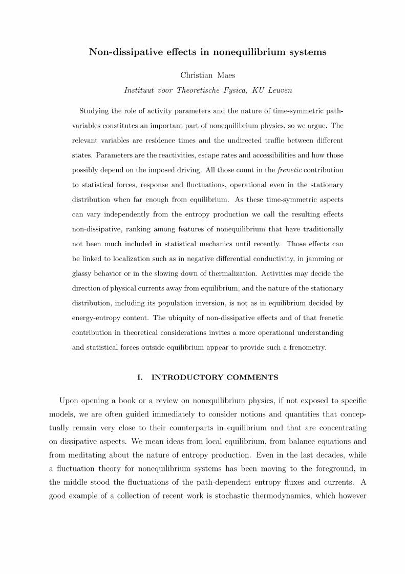
for normalization z := (α + δ + γ + κ)(δ + γ + κ + γ(δ + κ) + α(1 + δ + κ)). Clearly, from
symmetries and from normalization, such distribution is completely decided from knowing
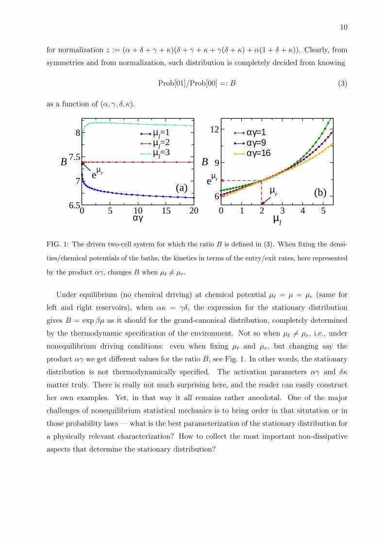
Prob[01]/Prob[00] =: B (3)
as a function of (α, γ, δ, κ).
0 5 10 15 20αγ
6.5
7
7.5
8
B
µl=1
µl=2
µl=3
0 1 2 3 4 5µ
l
6
9
12
B
αγ=1αγ=9αγ=16
(a)e
µr
µr
eµ
r
(b)
FIG. 1: The driven two-cell system for which the ratio B is defined in (3). When fixing the densi-
ties/chemical potentials of the baths, the kinetics in terms of the entry/exit rates, here represented
by the product αγ, changes B when µ` 6= µr.
Under equilibrium (no chemical driving) at chemical potential µ` = µ = µr (same for
left and right reservoirs), when ακ = γδ, the expression for the stationary distribution
gives B = exp βµ as it should for the grand-canonical distribution, completely determined
by the thermodynamic specification of the environment. Not so when µ` 6= µr, i.e., under
nonequilibrium driving conditions: even when fixing µ` and µr, but changing say the
product αγ we get different values for the ratio B, see Fig. 1. In other words, the stationary
distribution is not thermodynamically specified. The activation parameters αγ and δκ
matter truly. There is really not much surprising here, and the reader can easily construct
her own examples. Yet, in that way it all remains rather anecdotal. One of the major
challenges of nonequilibrium statistical mechanics is to bring order in that situtation or in
those probability laws — what is the best parameterization of the stationary distribution for
a physically relevant characterization? How to collect the most important non-dissipative
aspects that determine the stationary distribution?
11
The above example is easy but stands for the general scenario that static fluctuations in
the stationary distribution far from equilibrium will depend on activity parameters, and in
contrast with equilibrium, are not directly related to thermodynamics like via energy-entropy
like quantities. Still, when the model above is extended to the boundary driven exclusion
process, and one looks in the diffusive scaling limit (of space-time) one finds nonequilibrium
free energies which retain important nonequilibrium characteristics but the dependence on
the kinetics is gone. Clearly the precise formulae will be difficult to get analytically1, but
the general structure for the probability of a density profile is
ProbN [ρ(r), r ∈ [0, 1]] ' exp(−NI[ρ(r), r ∈ [0, 1]]) (4)
where I is called the nonequilibrium free energy and N is the rescaling parameter (e.g. the
size of the system in microscopic units). Here it is for the open symmetric exclusion process,
[26, 31], just for completeness,
I[ρ(r), r ∈ [0, 1]] =
∫ 1
0
dr
[ρ(r) log
ρ(r)
F (r)+ (1− ρ(r)) log
1− ρ(r)
1− F (r)+ log
F ′(r)
ρ1 − ρ0
]where the function F is the unique solution of
ρ(r) = F (r) +F (r)(1− F (r))F ′′(r)
(F ′(r))2, F (0) = ρ0, F (1) = ρ1
Note that on that hydrodynamic scale the fluctuations indeed do not appear to depend on
the details of the kinetics in terms of the exit and entry parameters at the edges; only the
densities ρ0, ρ1 of the left and right particle reservoirs count in the fluctuation functional
I, no matter whether the reservoirs contain champagne or water. Yet that disappearing
of the relevant role of activity parameters is restricted to the diffusive regime and to the
macroscopic fluctuation theory we alluded to in the beginning of the introduction of these
notes.
A. The difference between a lake and a river
We mentioned above that for (global) detailed balance the equilibrium distribution
ρeq does not depend on the activity parameters ψ(x, y). In fact, in equilibrium if all
1 But there is some algorithm, where the static fluctuation functional becomes the solution of a Hamilton-
Jacobi equation, see [24, 25]. In equilibrium we have the macroscopic static fluctuation theory of
Boltzmann-Planck-Einstein. It is still very instructive to read the first pages of [27] to get an early
review. Later reviews for the macroscopic fluctuation theory in equilibrium are for example [28–30].
12
states in K remain connected via some transition path, adding kinetic constraints (i.e.,
imposing ψ(x, y) = 0 for some (x, y)) has no effect on the stationary distribution; we retain
ρeq(x) ∝ exp−F(x). Leaving even aside the required irreducibility, by isolating parts of
the state space which are no longer accessible when not starting in it, locally the stationary
distribution really does not change drastically. For example we can look at the dynamics
on fewer states, like restricting to smaller volume and ask how the stationary distributions
resemble. The answer is well known, under detailed balance the stationary distribution
for the smaller volume (on a restricted class of states) is the restriction of the equilibrium
distribution on the larger volume (original state space), possibly with some changes at the
boundary only. In other words, if a big lake gets perturbed by a wall in the middle, there
just appear two (very similar) lakes.
In nonequilibrium, setting some activity parameters ψ(x, y) to zero can have drastic
effects. For example, suppose we have a ring K = ZN , x = 1, 2, . . . , N with N + 1 = 1,
with transition rates k(x, x + 1) = p, k(x, x − 1) = q (random walker on a ring). Then the
uniform distribution ρ(x) = 1/N is invariant for all values of p and q. Let us now break the
ring by putting k(1, N) = 0 = k(N, 1). The dynamics remains well defined and irreducible
on the same state space K but now the stationary distribution is
ρ(x) ∝(p
q
)xand only in equilibrium, for p = q, is the stationary distribution (unchanged) uniform. For
nonequilibrium, at driving log p/q 6= 0, the uniform distribution has changed into a spatially
exponential profile. Throwing a tree or building a wall in a river has a much larger effect
than for a lake. The river can even turn into a lake.
In the next section we give an example how you can use the activity parameters to select
one or more states for the stationary distribution to be concentrated on.
B. From the uniform to a peaked distribution
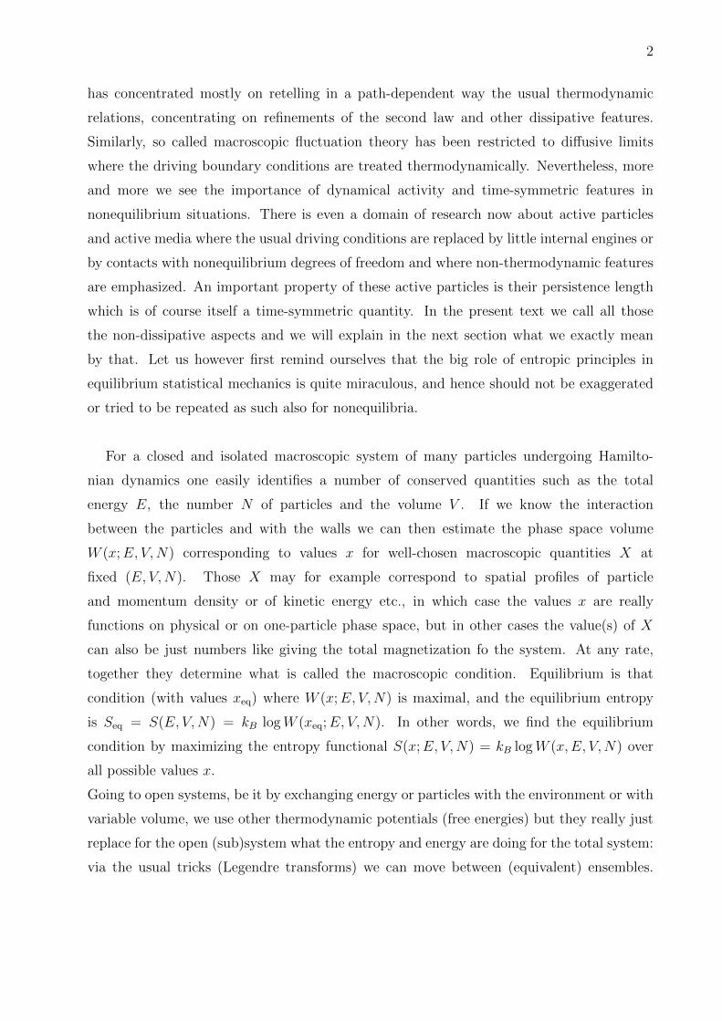
Suppose a three-state Markov process with state space K = {1, 2, 3} and transition rates,
k(1, 2) = a eε/2, k(2, 3) = b eε/2, k(3, 1) = c eε/2,
k(1, 3) = c e−ε/2, k(3, 2) = b e−ε/2, k(2, 1) = a e−ε/2 (5)
13
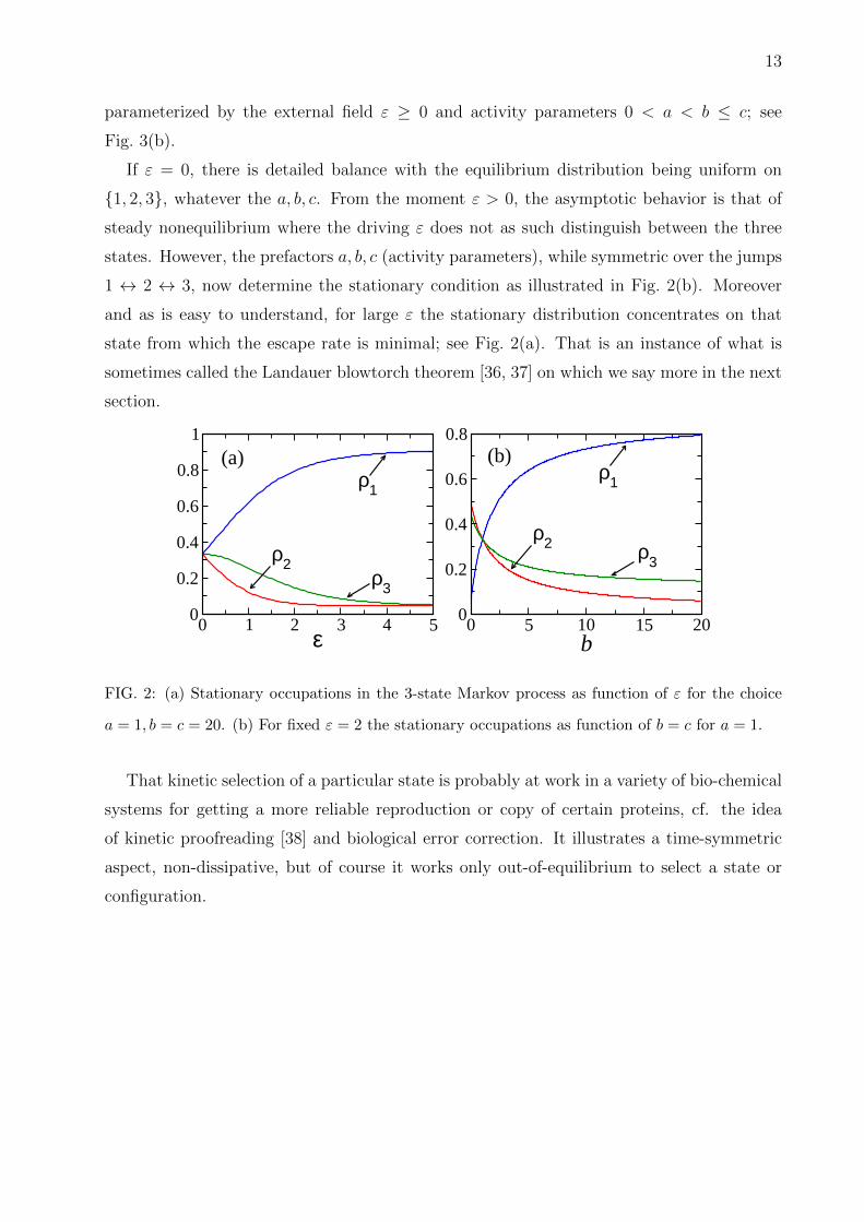
parameterized by the external field ε ≥ 0 and activity parameters 0 < a < b ≤ c; see
Fig. 3(b).
If ε = 0, there is detailed balance with the equilibrium distribution being uniform on
{1, 2, 3}, whatever the a, b, c. From the moment ε > 0, the asymptotic behavior is that of
steady nonequilibrium where the driving ε does not as such distinguish between the three
states. However, the prefactors a, b, c (activity parameters), while symmetric over the jumps
1 ↔ 2 ↔ 3, now determine the stationary condition as illustrated in Fig. 2(b). Moreover
and as is easy to understand, for large ε the stationary distribution concentrates on that
state from which the escape rate is minimal; see Fig. 2(a). That is an instance of what is
sometimes called the Landauer blowtorch theorem [36, 37] on which we say more in the next
section.
0 1 2 3 4 5ε
0
0.2
0.4
0.6
0.8
1
0 5 10 15 20b
0
0.2
0.4
0.6
0.8(a) (b)
ρ1
ρ2
ρ1
ρ2 ρ3ρ3
FIG. 2: (a) Stationary occupations in the 3-state Markov process as function of ε for the choice
a = 1, b = c = 20. (b) For fixed ε = 2 the stationary occupations as function of b = c for a = 1.
That kinetic selection of a particular state is probably at work in a variety of bio-chemical
systems for getting a more reliable reproduction or copy of certain proteins, cf. the idea
of kinetic proofreading [38] and biological error correction. It illustrates a time-symmetric
aspect, non-dissipative, but of course it works only out-of-equilibrium to select a state or
configuration.
14
C. Heat bounds
Let us go back to (1) but now write the entropy flux as heat over environment tempera-
ture,
k(x, y) := ψ(x, y) exp[β
2q(x, y)
](6)
where we took β = (kBT )−1 ≥ 0 for the inverse temperature of the environment so that
the heat is q(x, y) = −q(y, x) following the prescription of local detailed balance (1),
s(x, y) = βq(x, y). The activity parameters are ψ(x, y) = ψ(y, x) ≥ 0. The edges of K (as a
graph) are made by the pairs {x, y} over which ψ(x, y) > 0.
We want to understand the stationary occupations ρ(x) in terms of the heat {q(x, y)} and
activity parameters {ψ(x, y)}.
For any oriented path D along the edges b = (x, y), let q(D) be the total dissipated heat
along D, which is the sum q(D) :=∑
b q(b). For a spanning tree T we put Txy for the unique
oriented path from x to y along the edges of T . Then, we show in [37] that the stationary
occupations satisfy
minyD→xq(D) ≤ 1
βlog
ρ(x)
ρ(y)≤ max
yD→xq(D) (7)
with the minimum and maximum taken over all oriented paths (self-avoiding walks) from y to
x on the graph. In the case of global detailed balance q(x, y) = F(x)−F(y) we have that the
heat q(D) = F(xi)−F(xf ) only depends on the initial and final configurations xi, xf of the
path D. We then get the Boltzmann equilibrium statistics for ρ. However in nonequilibrium
systems, most of the time it is easy to find configurations x and y for which there exist two
oriented paths D1,2 from x to y such that q(D1) < 0 < q(D2) (heat-incomparable). In other
words along one path D2 heat is dissipated while transiting from x to y, while along the
other path D1 heat is absorbed to go from x to y. Then, it simply cannot be decided which
of the occupations ρ(x), ρ(y) is larger on the basis of heat functions q(x, y); we only have
the heat bounds (7) and nothing more can be concluded from dissipative characteristics.
The activity parameters then become essential. In such a case indeed where a pair of states
x∗ and y∗ is “heat-incomparable”, then without changing the heat function {q(x, y)}, we
can always make either ρ(x∗) > ρ(y∗) or ρ(x∗) < ρ(y∗) by just changing the {ψ(x, y)}.That is typical in nonequilibrium systems; we cannot (partially) order states depending on
whether heat is being released over all paths connecting them, or being absorbed over all
paths connecting them. In such a case, when depending on what path we choose heat is
15
absorbed or released in going x → y, then we can change the relative weight ρ(x)/ρ(y) in
the stationary distribution ρ from being greater than one to being smaller than one, just
by an appropriate change in the activity parameters (the a, b, c in the previous section).
To all that we can add that the heat bounds (7) become less sharp of course when the
environment temperature lowers (high β). We can then expect that the notion of ground
state for nonequilibrium systems is not at all (only) energy-connected but also takes into
account non-dissipative aspects such as accessibility; see [32, 33].
D. Population inversion
Thermal equilibrium occupation statistics is completely determined by energy-entropy
considerations. In the simplest case of a nondegenerate multilevel system, we have relative
occupations determined by temperature and energy difference. However, when adding
kinetic effects, like introducing a symmetrizer between two levels we break detailed balance
and we can basically select any desired (even high) energy level to have the largest
occupation. In that way, like for lasers, under nonequilibrium conditions but via changes in
non-dissipative factors, we can establish an inversion of the population with respect to the
usual Boltzmann statistics.
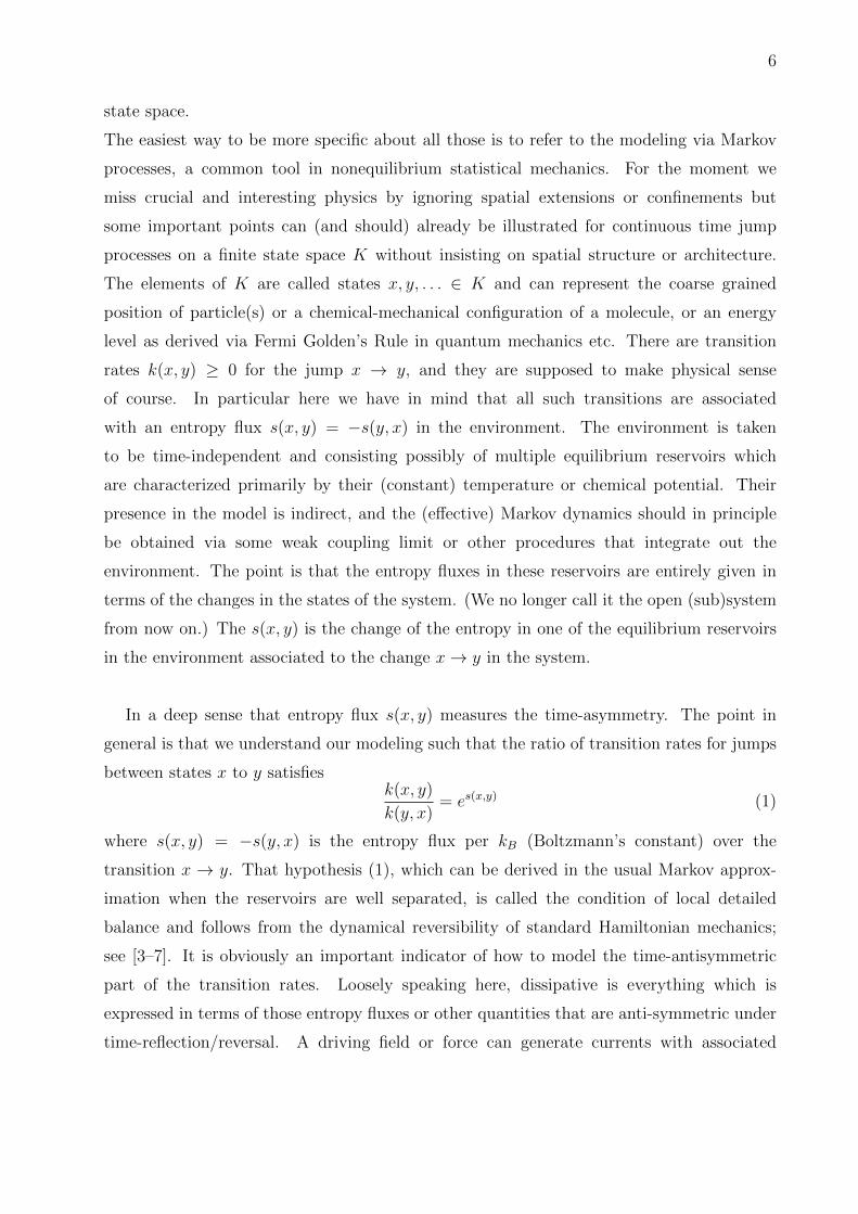
Consider a system with K energy levels where the lowest and highest levels are connected
by an equalizer and an additional energy barrier F exists between the K and K − 1th level.
Denote the number of particles at level ` by n` and let the rate at which a single particle
jumps from level ` to level `′ be k(`, `′) with
k(`, `+ 1) = n` e− 1T
(E`+1−E`), ∀` 6= K − 1, K
k(`, `− 1) = n`, ∀` 6= K, 1
k(K − 1, K) = nK−1 e−FT e−
1T
(EK−EK−1), k(1, K) = b n1
k(K,K − 1) = nK e−FT , k(K, 1) = b nK (8)
The equalizing symmetric activity parameter b > 0 between the highest and lowest energy
level along with the factor e−F/T gives rise to the desired population inversion [32]. That
can be witnessed by the “effective temperature”
Teff = (EK − E1)
[log
ρ1
ρK
]−1
(9)
16
0 0.5 1 1.5b
0
10
20
30
Teff
F=2,T=1F=2,T=5F=3,T=1F=3,T=5
(a)
1
23
(b)
aeε/2
ae−ε/2ce−ε/2ceε/2
beε/2
be−ε/2
FIG. 3: (a) Effective temperature Teff as function of the symmetrizer b for different environment
temperatures T and barrier strengths F for K = 3 levels. For b = 0 there is no dependence on F .
For lower T and b > 0 the dependence on F shows more. (b) Graph-representation of the 3-state
Markov process (5). Changing the activity parameters a, b, c can select a state when ε > 0 is big
enough.
Fig. 3(a) (a variation of Fig. 7(a) in [35]) shows that the effective temperature Teff is in-
creasing with the strength of the equalizer b. At low temperature T the effective temperature
Teff will grow fast with b (and for high T the effective Teff is about constant). That shows
up in the figure: for a fixed F, the curve of Teff corresponding to a lower thermodynamic
temperature T crosses that of a higher temperature from below. That signifies population
inversion as function of the activity parameter b for low temperature T . The barrier F
(again time-symmetric) facilitates that phenomenon — crossing occurs for smaller b when
F is increased.
E. Variational principles
Static fluctuations refer to the occurrence of single time events that are not typical for
an existing condition. For example, in this room there is a certain air density which is
quite homogeneous and as a result we have a constant index of refraction of light etc. That
is typical for the present equilibrium condition here for air at room temperature and at
atmospheric pressure. Yet, there are fluctuations, meaning little regions where the density
locally deviates. We can expect these regions to be very small; otherwise we would have
noticed before. That is why such fluctuations are called large deviations; they are very
unlikely when they take macroscopic proportions and they are exponentially small in the
17
volume of the fluctuation. The rate of fluctuations, i.e., what multiplies that volume, is given
by the appropriate free energy difference (at least in equilibrium); for the local air density
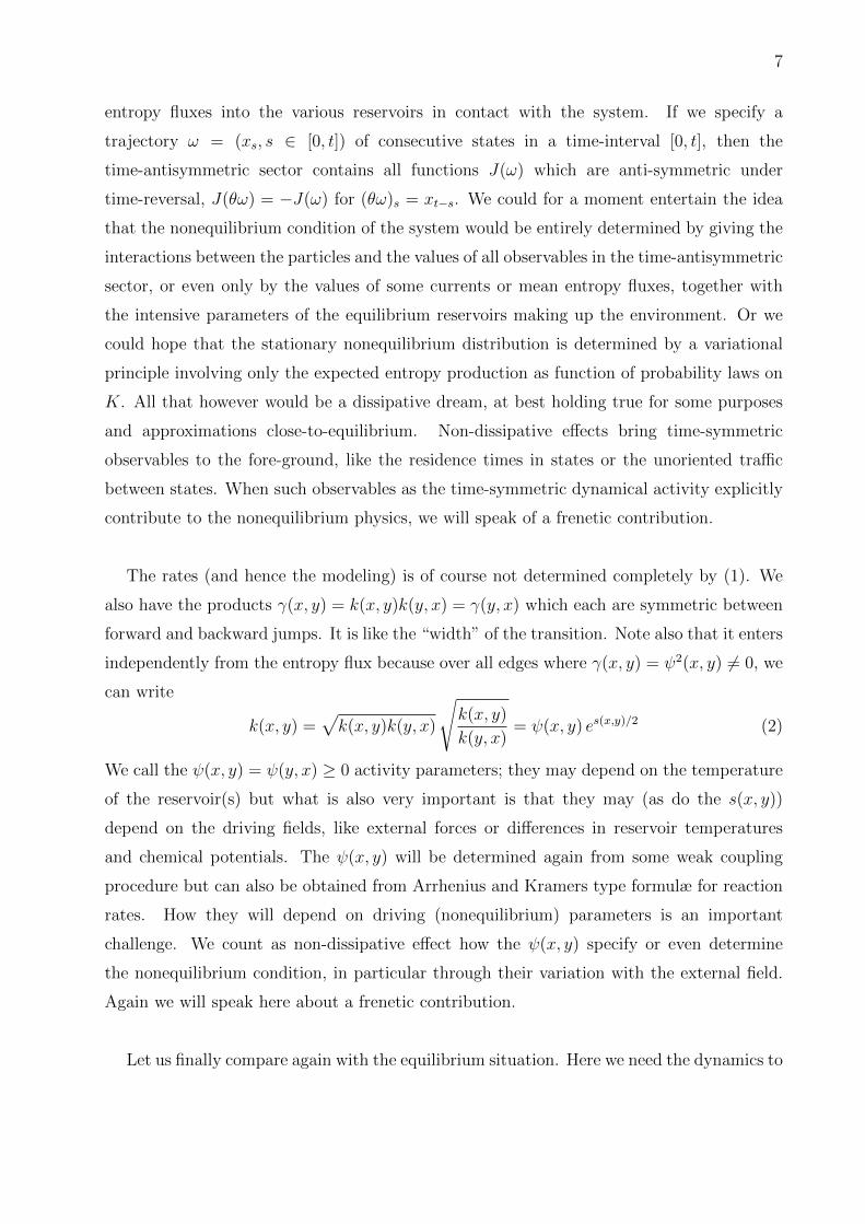
we would have the grand canonical potential. Similarly, the energy EV in a subvolume V
fluctuates. The total energy is conserved in an isolated system, but there will be exchanges
through the boundary; see Fig. 4. It could be that the particle number N is also fixed
inside V , in which case the fluctuations are governed by the Helmholtz free energy F , in the
following sense. When the system is in thermal equilibrium and away from phase coexistence
regimes2 the local fluctuations of the energy density EV /V satisfy the asymptotic law
Prob
[EVV
= e
]' exp−βV [F(e)−Feq] (10)
where the variational functional is F(e) = e−TS(e, V,N) with S being the entropy density
at that energy density e, and Feq(T, V,N) being the equilibrium free energy density at
temperature T (and β−1 = kBT ).
V,N
T
FIG. 4: Fluctuations in a subvolume V in weak contact with an equilibrium bath at fixed temper-
ature T are described in the canonical Gibbs ensemble.
It is only a slight variation to ask for the probability of profiles, i.e., to estimate the
plausibility of given spatial variations of a particular quantity. We then need spatially
extended systems, most interestingly with interacting components and that is what we
already did around formula (4).
2 Otherwise, we must introduce also surface tensions and the scaling could be with the surface of the
subsystem and not with its volume.
18
As a clear consequence of fluctuation formulæ as (10) we get that the equilibrium con-
dition minimizes the free energy functional, F(e) in the above. That constitutes in fact
a derivation of the Gibbs variational principle. As such, one could try to repeat that for
nonequilibrium systems, but clearly such a formulation with explicit functionals does not
exist (yet). Since a long time however people have been trying to use a dissipative charac-
terization of the stationary distribution. These are known as entropy production principles;
see the minimum entropy production principle discussed in [10].
The entropy production rate functional corresponding to the Markov process characterized
by (2) is
σ(µ) =∑x,y
µ(x)k(x, y) logk(x, y)µ(x)
k(y, x)µ(y)≥ 0 (11)
defined on all (possibly even unnormalized) distributions µ. That functional σ is convex, and
homogeneous, σ(λµ) = λσ(µ). In our case of irreducible Markov processes it is even strictly
convex. It thus has a unique minimum, called the Prigogine distribution ρP > 0. Suppose
now that k(x, y) = kε(x, y) depends on a driving parameter ε so that there is detailed balance
for ε = 0, k0(x, y) = keq(x, y), with smooth dependence on ε close to equilibrium. Then, the
stationary distribution ρ(ε) and the Prigogine distribution ρ(ε)P coincide up to linear order
in ε: ρ(ε)P = ρ(ε) + O(ε2). That is called the minimum entropy production principle (here
formulated for finite state space Markov jump processes). It should be added that most
often, the Prigogine distribution as completely characterized by minimizing the entropy
production rate (11) is of course not equal to the (true) stationary distribution and they
really start to differ from second order onwards. The reason is just a non-dissipative effect.
For a discussion on maximum entropy production principles, we refer to [34].
F. Recent examples
1. Demixing
The above examples are extremely simple, but the heuristics can easily be moved towards
more interesting applications. Suppose indeed that we have a macroscopic system with two
types of particles and we must see whether a condition with phase separation between the
two types is most plausible. In equilibrium that would be called a low-entropy condition
which can only be obtained at sufficiently low temperature and with the appropriate interac-
tions. In nonequilibrium opens the possibility of a totally different physics, that the demixed
19
configuration gets more plausible whenever it is a trap in the sense that the escape rates to
leave from it are rather low. For that to be effective, we need, as above in Section III C,
that the mixed and the demixed condition are dynamically connected through both positive
dissipative as well as negative dissipative paths. In the end it will be the configuration with
lowest escape possibilities that will dominate.
An example of that phenomenon is shown in [39, 40]. The importance of life-time consider-
ations especially at low temperatures is discussed in [32].
2. No thermodynamic pressure
Suppose we have active particles in a container, like for active Brownians or for self-
propelled particles etc. The pressure on a wall is obtained from calculating the mechanical
force on the wall and to average over the stationary ensemble. Since that stationary ensem-
ble could depend on kinetic details, we cannot expect the pressure to be thermodynamically
determined. It means that details of the interaction between particles and wall can matter
and that, unless we have symmetries that cancel the kinetic dependencies, we will not have
an equation of state relating that wall pressure to bulk properties such as global density or
temperature. The simple reason is that the stationary distribution is itself not thermody-
namically energy-entropy characterized.
We find an analysis of that effect in [41].
IV. TRANSPORT PROPERTIES
Transport is usefully characterized in terms of response coefficients such as conductivities.
We discuss them in Section V, while here we deal with the question of what determines the
direction of the current and how it could decrease by pushing harder.
A. Current direction decided by time-symmetric factors
Consider the metal rod in Fig. 5 which is connected at its ends with a hot and a cold ther-
mal bath. The environment exchanges energy with the system but at different temperatures
for the two ends of the rod.
In that case we can, on the appropriate scale of time, think of the system as being in
steady nonequilibrium. It is stationary alright, not changing its macroscopic appearance, but
20
FIG. 5: Example of a simple stationary current for which the direction is decided by the positivity
of the entropy production.
a current is maintained through it. Therefore the (stationary) system is not in equilibrium.
In fact there is a constant production σ of entropy in the environment, in the sense that
energy is dissipated in the two thermal baths. We apply the usual formula
σ = J1/T1 + J2/T2
with Ji the energy flux into the i−th bath at temperature Ti. Stationarity (conservation of
energy) implies that J1 + J2 = 0 so that we can find the direction of the energy current J1
by requiring
σ = J1(1/T1 − 1/T2) ≥ 0 (second law)
Similar scenario’s can be written for chemical and mechanical baths that frustrate the
system. Those are typical examples where, to find the direction of the current, we can
apply the second law stating that the stationary entropy production be positive3.
It is however not uncommon in nonequilibrium to find a system where the direction of the
current is essentially not decided by the entropy production. The paper [2] treats different
examples of that.
A simple scenario is to imagine a network consisting of various nodes (vertices) repre-
senting each a certain chemical-mechanical configuration of an ensemble of molecules or
the coarse-grained positions of diffusing colloids. The edges between the nodes indicate the
possible transitions (jumps) in a continuous time Markov dynamics. There could be various
cycles in that network and some of them relate to the observed or interesting physical or
chemical current. The question is what typically will be the direction of that current in that
cycle; is it e.g. clockwise or counter-clockwise in the network, which could imply a different
direction of the current in physical space.
3 In the presence of multiple currents we can only require that the matrix of Onsager response coefficients
is positive.
21
To be more specific let us look at Fig. 6, where we see an example of a necklace, a periodic
repetition of pearls. Think of a random walker jumping between the nodes connected via
an edge. Let us suppose we are interested in the current going in the bulk necklace (the red
nodes). The problem becomes non-trivial at the moment we organize the driving in each
pearl in such a way that “entropically” there is no preferred direction.
A
B
Connection points
FIG. 6: A necklace consists of pearls, here heptagons connected periodically at the red nodes.
A clockwise current is generated in each pearl in such a way that the upper A-trajectory has the
same dissipation as the lower B-trajectory. Nevertheless a current typically appears in the necklace.
Courtesy of Mathias Stichelbaut.
The simplest example is represented in Fig. 7 where the pearls are triangles. We specify
the transition rates as follows:
k↗ = eε/2, k↘ = eε/4, k← = ϕ eε/2
k↙ = e−ε/2, k↖ = e−ε/4, k→ = ϕ e−ε/2 (12)
where the arrows reflect the direction of the hopping in each triangle of Fig. 7. The ϕ is an
activity parameter. We have chosen the rates in such a way that the trajectory A =↗↘has entropy flux
S(A) = logk↗ k↘k↖ k↙
= ε
identical to the entropy flux over trajectory B =←, S(B) = log k←k→
= ε.
22
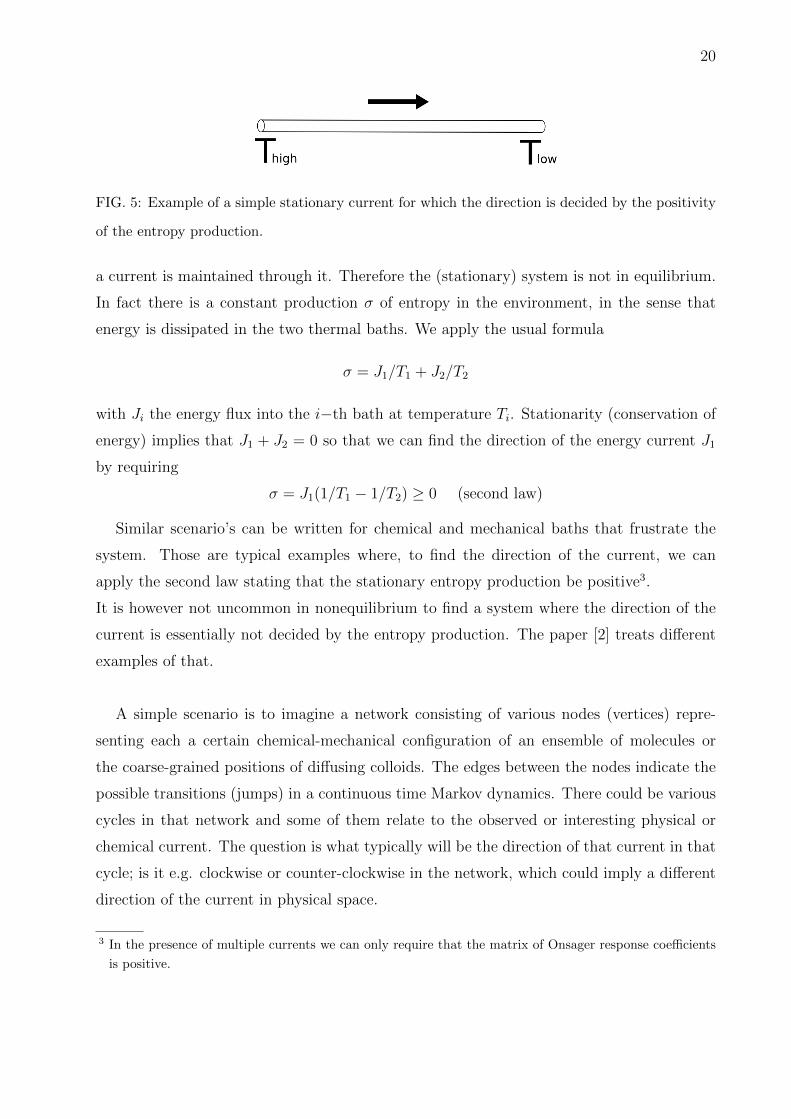
FIG. 7: Zooming in on the triangular pearls making the closed necklace. Will the current go left
or right over the lower nodes when an emf with driving ε in (12) is created in each triangle which
is entropically neutral? Courtesy of Mathias Stichelbaut.
Many other choices are possible of course to achieve that. Note that the entropy flux
balance between A and B is independent of ϕ which is a time-symmetric parameter in the
sense that k←k→ = ϕ2. A non-dissipative effect would be to see how changes in ϕ influence
the nonequilibrium nature of the system, here in particular, how it can decide the direction
of the necklace current. And in fact it does: for a fixed driving ε, by changing ϕ we can
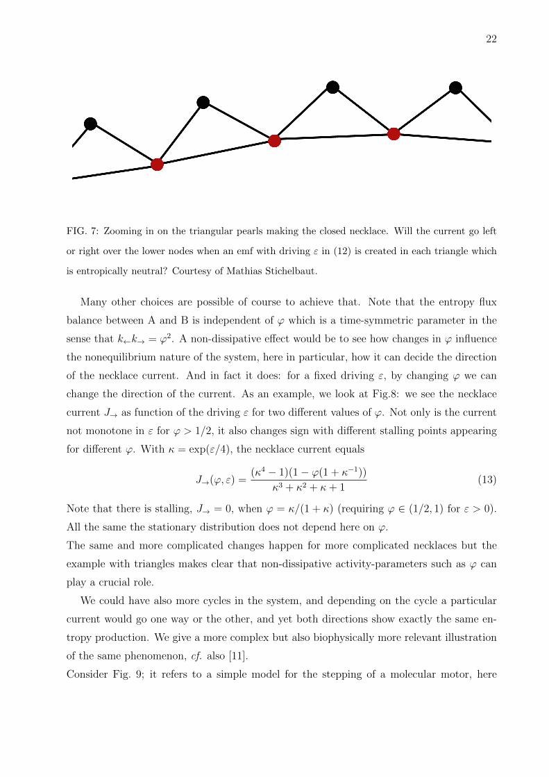
change the direction of the current. As an example, we look at Fig.8: we see the necklace
current J→ as function of the driving ε for two different values of ϕ. Not only is the current
not monotone in ε for ϕ > 1/2, it also changes sign with different stalling points appearing
for different ϕ. With κ = exp(ε/4), the necklace current equals
J→(ϕ, ε) =(κ4 − 1)(1− ϕ(1 + κ−1))
κ3 + κ2 + κ+ 1(13)
Note that there is stalling, J→ = 0, when ϕ = κ/(1 + κ) (requiring ϕ ∈ (1/2, 1) for ε > 0).
All the same the stationary distribution does not depend here on ϕ.
The same and more complicated changes happen for more complicated necklaces but the
example with triangles makes clear that non-dissipative activity-parameters such as ϕ can
play a crucial role.
We could have also more cycles in the system, and depending on the cycle a particular
current would go one way or the other, and yet both directions show exactly the same en-
tropy production. We give a more complex but also biophysically more relevant illustration
of the same phenomenon, cf. also [11].
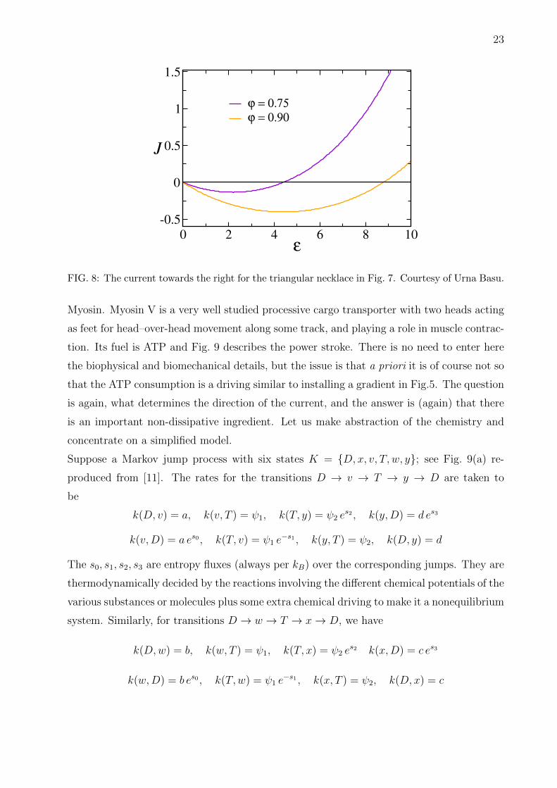
Consider Fig. 9; it refers to a simple model for the stepping of a molecular motor, here
23
0 2 4 6 8 10
ε
-0.5
0
0.5
1
1.5
J
ϕ = 0.75
ϕ = 0.90
FIG. 8: The current towards the right for the triangular necklace in Fig. 7. Courtesy of Urna Basu.
Myosin. Myosin V is a very well studied processive cargo transporter with two heads acting
as feet for head–over-head movement along some track, and playing a role in muscle contrac-
tion. Its fuel is ATP and Fig. 9 describes the power stroke. There is no need to enter here
the biophysical and biomechanical details, but the issue is that a priori it is of course not so
that the ATP consumption is a driving similar to installing a gradient in Fig.5. The question
is again, what determines the direction of the current, and the answer is (again) that there
is an important non-dissipative ingredient. Let us make abstraction of the chemistry and
concentrate on a simplified model.
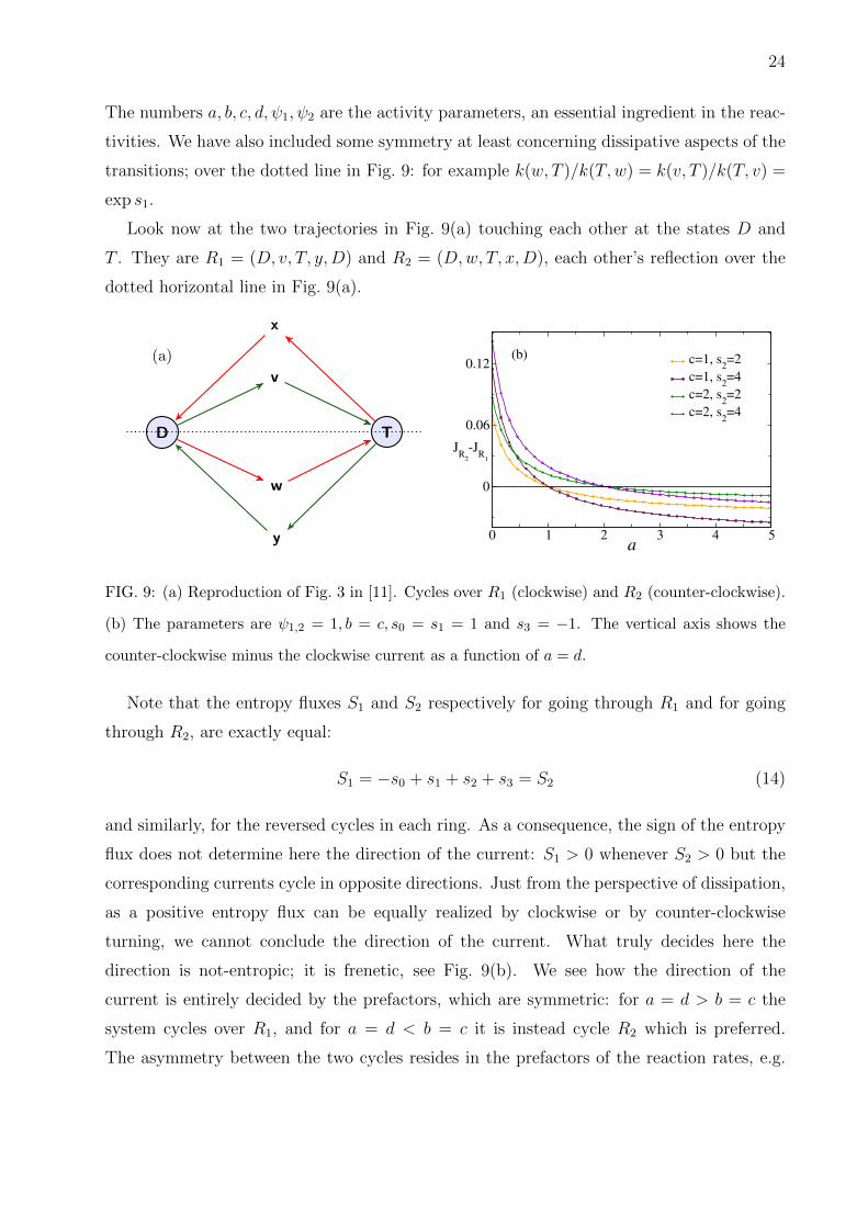
Suppose a Markov jump process with six states K = {D, x, v, T, w, y}; see Fig. 9(a) re-
produced from [11]. The rates for the transitions D → v → T → y → D are taken to
be
k(D, v) = a, k(v, T ) = ψ1, k(T, y) = ψ2 es2 , k(y,D) = d es3
k(v,D) = a es0 , k(T, v) = ψ1 e−s1 , k(y, T ) = ψ2, k(D, y) = d
The s0, s1, s2, s3 are entropy fluxes (always per kB) over the corresponding jumps. They are
thermodynamically decided by the reactions involving the different chemical potentials of the
various substances or molecules plus some extra chemical driving to make it a nonequilibrium
system. Similarly, for transitions D → w → T → x→ D, we have
k(D,w) = b, k(w, T ) = ψ1, k(T, x) = ψ2 es2 k(x,D) = c es3
k(w,D) = b es0 , k(T,w) = ψ1 e−s1 , k(x, T ) = ψ2, k(D, x) = c
24
The numbers a, b, c, d, ψ1, ψ2 are the activity parameters, an essential ingredient in the reac-
tivities. We have also included some symmetry at least concerning dissipative aspects of the
transitions; over the dotted line in Fig. 9: for example k(w, T )/k(T,w) = k(v, T )/k(T, v) =
exp s1.
Look now at the two trajectories in Fig. 9(a) touching each other at the states D and
T . They are R1 = (D, v, T, y,D) and R2 = (D,w, T, x,D), each other’s reflection over the
dotted horizontal line in Fig. 9(a).
v
D
w
T
x
y
(a)
0 1 2 3 4 5a
0
0.06
0.12
JR
2
-JR
1
c=1, s2=2
c=1, s2=4
c=2, s2=2
c=2, s2=4
(b)
FIG. 9: (a) Reproduction of Fig. 3 in [11]. Cycles over R1 (clockwise) and R2 (counter-clockwise).
(b) The parameters are ψ1,2 = 1, b = c, s0 = s1 = 1 and s3 = −1. The vertical axis shows the
counter-clockwise minus the clockwise current as a function of a = d.
Note that the entropy fluxes S1 and S2 respectively for going through R1 and for going
through R2, are exactly equal:
S1 = −s0 + s1 + s2 + s3 = S2 (14)
and similarly, for the reversed cycles in each ring. As a consequence, the sign of the entropy
flux does not determine here the direction of the current: S1 > 0 whenever S2 > 0 but the
corresponding currents cycle in opposite directions. Just from the perspective of dissipation,
as a positive entropy flux can be equally realized by clockwise or by counter-clockwise
turning, we cannot conclude the direction of the current. What truly decides here the
direction is not-entropic; it is frenetic, see Fig. 9(b). We see how the direction of the
current is entirely decided by the prefactors, which are symmetric: for a = d > b = c the
system cycles over R1, and for a = d < b = c it is instead cycle R2 which is preferred.
The asymmetry between the two cycles resides in the prefactors of the reaction rates, e.g.
25
a 6= b for the transition D → v versus D → w. When there is detailed balance, i.e. for
s0 = s1 + s2 + s3, the discrepancy a� b or c 6= d etc. is irrelevant and the stationary regime
would be equilibrium-dead showing no orbiting whatsoever. Those activity considerations
for the nonequilibrium statistical mechanical aspects of Myosin V motion are discussed in
[11]. General considerations on how dynamical activity plays in determining the direction
of ratchet currents are found in [12].
B. Negative differential conductivity
The usual way random walks are discussed is by giving the rates for the walker to move to
its neighbors. Let us then take the simple 1-dimensional walk, x ∈ Z, with rates k(x, x+1) =
p and k(x, x− 1) = q. The fact that p > q would mean that there is a bias to move to the
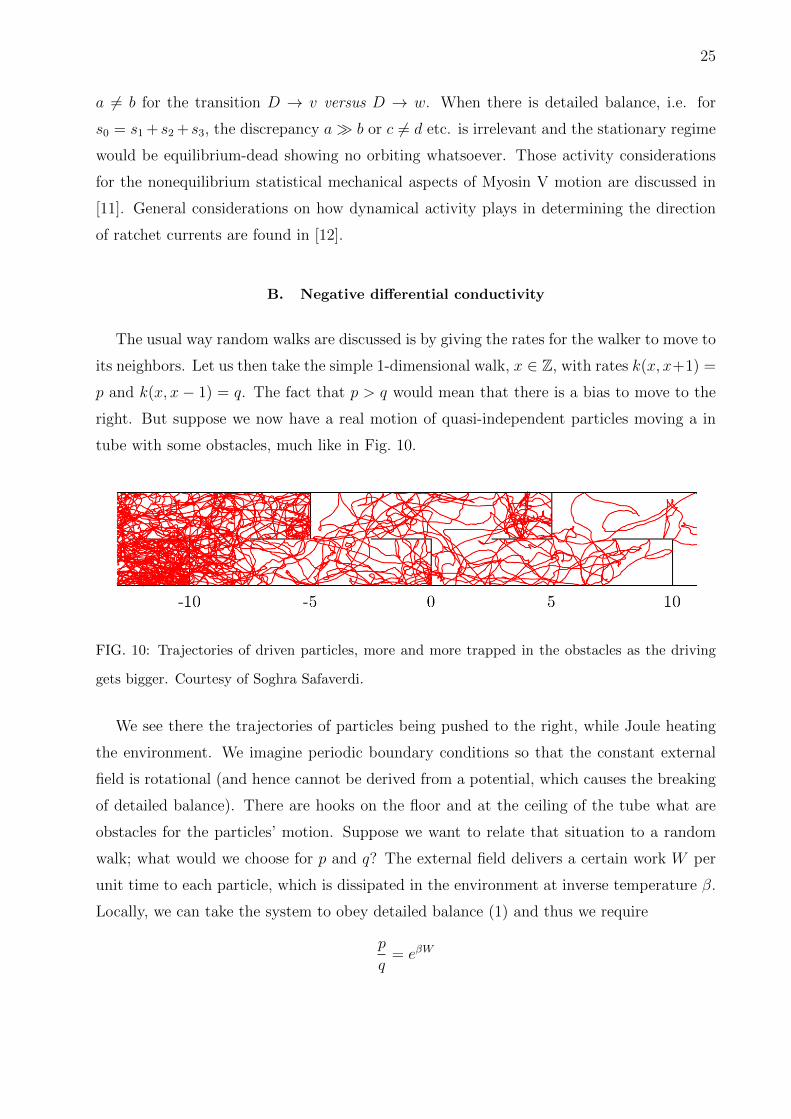
right. But suppose we now have a real motion of quasi-independent particles moving a in
tube with some obstacles, much like in Fig. 10.
FIG. 10: Trajectories of driven particles, more and more trapped in the obstacles as the driving
gets bigger. Courtesy of Soghra Safaverdi.
We see there the trajectories of particles being pushed to the right, while Joule heating
the environment. We imagine periodic boundary conditions so that the constant external
field is rotational (and hence cannot be derived from a potential, which causes the breaking
of detailed balance). There are hooks on the floor and at the ceiling of the tube what are
obstacles for the particles’ motion. Suppose we want to relate that situation to a random
walk; what would we choose for p and q? The external field delivers a certain work W per
unit time to each particle, which is dissipated in the environment at inverse temperature β.
Locally, we can take the system to obey detailed balance (1) and thus we require
p
q= eβW
26
That does not quite determine the rates p, q. What appears important here also is to know
how the escape rates depend on W ; that is the dependence
p+ q = ψ(W )
From the situation in Fig. 10 it is clear that a large driving field or what amounts to the
same thing, large W , causes trapping. The particles are being pushed against the hooks, or
caught and have much difficulty in escaping from the trap as they are constantly pushed
back on them. Hence the escape rates and the function ψ will be decreasing in W . In fact,
we can expect that here ψ(W ) ∼ exp−βW ; see [13].
Let us see what that means for the current; the random walker has a current
J = p− q = ψ(W )1− e−βW1 + e−βW
(15)
We clearly see that for large W , in fact basically outside the linear regime in W , the current
becomes decreasing in W (whenever ψ is decreasing in W ); the more you push the more
the particles get trapped and the current goes down; see also [14].
The above mechanism, described here in the simplest possible terms, is an instance of
negative differential conductivity, the current showing a negative derivative with respect to
the driving field. It is physically interesting and also very important, but for us it suffices
to remark that the effect is clearly non-dissipative. Of course one needs a current in the
first place but what happens with it is related to time-symmetric fluctuations, here in the
form of waiting time distributions. The dynamical activity is a function of W and cannot
be ignored, and is even essential in the understanding of the effect of negative differential
conductivities. We have a general response–approach to that effect coming up in Section
V; see (25)–(27).
As a final remark, the trapping effect in the above is trivially caused by the geometry.
There are other mechanisms like in the Lorentz gas where the obstacles are random placed
or even moving slightly, [15–17]. But we can also imagine that that trapping and caging is
not caused by external placements but by the interaction itself between the driven particles.
In that case we speak about jamming and glass transitions [22], or even about many body
localization [23].
27
C. Death and resurrection of a current
The previous section can be continued to the extreme situation where the current
actually dies (vanishes completely) at large but finite driving. That phenomenon has been
described in the probability and physics theory alike; see e.g. [18, 19]. Recently we showed
how the current can resurrect for those large field amplitudes by adding activity in the
form of a time-dependent external field, [20]. The cure is somewhat similar to a dynamical
counterpart of stochastic resonance, [21]. The point is that by the ‘shaking’ of the field,
particles get again time to go backwards and find new ways to escape. It is effectively
a resetting mechanism that improves the finding of the exit from the condition which
previously meant an obstacle.
One should imagine an infinite sequence of potential barriers (along a one-dimensional
line). There is an external field E which drives the particles to the right but at the same
time the height of the potential barriers grows with E. In other words we have again an
activity parameter (for escape over the barrier) here which decreases with E. Since there is
an infinite sequence of them the current to the right will vanish identically when the field E
reaches a threshold Ec. But suppose we now add a time-dependence and make the external
field E = Ef(t) where f(t) is periodic and∫ τ
0f(t)/τ = 1 over the period τ . The amplitude of
the force over the period has therefore not changed. Yet, we can increase the variance of f(t)
for fixed such amplitude, and hence the capacity of negative field will grow and the potential
barrier goes down, even compensating for the negative field, so that the particle can diffuse
through to the right. The result of that activation (the “shaking”) is the resurrection of the
current in the form of a first order phase transition (at zero temperature); see [20].
V. RESPONSE
We come to the meaning and the extension of the fluctuation–dissipation theorem.
The general aim is the physical understanding of the statistical reaction of a system to
an external stimulus. In that sense we look at averages of certain quantities, for example
over many repeated measurements. We start from a stationary condition and we perturb
the system over some time period. The question is to find a good representation of the
response of the system: we want to learn what determines the susceptibility in terms of the
original (unperturbed) system. Old examples are the Sutherland-Einstein relation between
28
diffusion and mobility, or the Nyquist-Johnson formula for the thermal noise in resistors.
These can be extended to nonequilibrium situations and invariantly specific non-dissipative
effects show up. Alternatively, measuring response can inform us about activity parameters
and time-symmetric traffic in the original system.
For the above purpose and especially for nonequilibrium systems, working on space-time
is more convenient than directly working on the single-time distribution. The path-space
distribution is local in space-time and has often explicit representations; we speak then
about dynamical ensembles and it is part of nonequilibrium statistical mechanics to learn
how they are specified and what they determine.
A. Standard fluctuation–dissipation relation
We start by describing the path-space approach for characterizing the response in equi-
librium. We here thus deviate from the usual rather formal analytic treatment which is on
the level of perturbations of the time-flow, e.g. via a Dyson formula for the perturbation of
semi-groups or unitary evolutions.
A dynamical ensemble gives the weight of a trajectory of system variables. Let ω denote
such a system trajectory over time-interval [0, t]. It could be the sequence of positions of an
overdamped colloid or the sequence of chemical or electronic states of a complex molecule
etc. We consider a path–observable O = O(ω) with expectation
〈O〉 =
∫D[ω]P (ω)O(ω) =
∫D[ω] e−A(ω) Peq(ω)O(ω) (16)
Here D[ω] is the notation, quite formally, for the volume element on path–space. The
perturbed dynamical ensemble is denoted by P and gets specified by an action A with
respect to the reference equilibrium ensemble Peq:
P (ω) = e−A(ω) Peq(ω)
At the initial time, say t = 0, the system is in equilibrium and the path-probability distri-
butions P and Peq differ (only) because P is the dynamically perturbed ensemble. Time-
reversibility of the equilibrium condition is the invariance Peq(θω) = Peq(ω) under time-
reversal θ, defined on paths ω = (xs, 0 ≤ s ≤ t) via
(θω)s = πxt−s
29
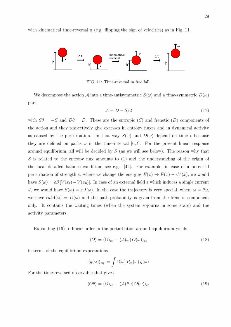
with kinematical time-reversal π (e.g. flipping the sign of velocities) as in Fig. 11.
FIG. 11: Time-reversal in free fall.
We decompose the action A into a time-antisymmetric S(ω) and a time-symmetric D(ω)
part,
A = D − S/2 (17)
with Sθ = −S and Dθ = D. These are the entropic (S) and frenetic (D) components of
the action and they respectively give excesses in entropy fluxes and in dynamical activity
as caused by the perturbation. In that way S(ω) and D(ω) depend on time t because
they are defined on paths ω in the time-interval [0, t]. For the present linear response
around equilibrium, all will be decided by S (as we will see below). The reason why that
S is related to the entropy flux amounts to (1) and the understanding of the origin of
the local detailed balance condition; see e.g. [42]. For example, in case of a potential
perturbation of strength ε, where we change the energies E(x)→ E(x)− εV (x), we would
have S(ω) = εβ [V (xt)−V (x0)]. In case of an external field ε which induces a single current
J , we would have S(ω) = ε J(ω). In the case the trajectory is very special, where ω = θω,
we have calA(ω) = D(ω) and the path-probability is given from the frenetic component
only. It contains the waiting times (when the system sojourns in some state) and the
activity parameters.
Expanding (16) to linear order in the perturbation around equilibrium yields
〈O〉 = 〈O〉eq − 〈A(ω)O(ω)〉eq (18)
in terms of the equilibrium expectations
〈g(ω)〉eq :=
∫D[ω]Peq(ω) g(ω)
For the time-reversed observable that gives
〈Oθ〉 = 〈O〉eq − 〈A(θω)O(ω)〉eq (19)
30
where we have used the time-reversibility Peq(θω) = Peq(ω) so that 〈g(ω)〉eq = 〈g(θω)〉eq.
Subtracting (19) from (18) gives
〈O −Oθ〉 = −〈[A(ω)−A(θω)]O(ω)〉eq
always to linear order in the perturbation. Now use that the time-anisymmetric part A(ω)−A(θω) = −S(ω) equals the entropy flux, to get
〈O −Oθ〉 = 〈S(ω)O(ω)〉eq (20)
for all path-variables O.
For an observable O(ω) = O(xt) that depends on the final time, we have Oθ(ω) = O(πx0).
Since 〈O(πx0)〉eq = 〈O(x0)〉eq = 〈O(xt)〉eq we receive
〈O(xt)〉 − 〈O(xt)〉eq = 〈S(ω)O(xt)〉eq (21)
In other words, the response is completely given by the correlation with the dissipative part
in the action, the entropy flux S. That result (21) is the Kubo formula even though it is
often presented in a more explicit way. Suppose indeed that the entropy flux is S(ω) =
εβ [V (xt) − V (x0)] (tiem-independent perturbation by a potential V starting at the initial
time zero) as mentioned above formula (18), then we would get from (21) that
〈O(xt)〉 = 〈O(xt)〉eq + εβ 〈[V (xt)− V (x0)]O(xt)〉eq + terms of order ε2
Similarly, for such a time-dependent (amplitude hs) perturbation that becomes
〈O(xt)〉 = 〈O(xt)〉eq + εβ
∫ t
0
ds hsd
ds〈V (xs)O(xt)〉eq + terms of order ε2 (22)
When the observable is odd under time-reversal, O(θω) = −O(ω) like O(ω) = S(ω) the
entropy flux itself, or when O(ω) = J(ω) is some time-integrated particle or energy current,
then we get from (20) the Green–Kubo formula
〈J〉 =1
2〈S(ω) J(ω)〉eq, and 〈S〉 =
1
2Vareq[S] (23)
That the linear order gets expressed as a correlation between the observable in question and
the entropic component S only is the very essence of the fluctuation–dissipation relation.
One can imagine different perturbations with the same S(ω) (dissipatively equivalent) and
there will the same linear response around equilibrium. Obviously, in the time-correlation
functions that enter the response, there are kinetic aspects and non-dissipative contributions
31
are thus present already in first order. Yet, there is no explicit presence of non-dissipative
observables. Again, even when the perturbation depends on kinetic and time-symmetric
factors, the linear response (21))–(22)–(23) erases that detailed dependence and only picks
up the thermodynamic dissipative part S. In particular, in equilibrium for the Gibbs distri-
butions the stationary distribution is just energy-entropy determined.
B. Enters dynamical activity
The previous section discussed the linear response around equilibrium (by using its time-
reversibility). Yet, the line of reasoning is essentially unchanged when doing linear response
around nonequilibrium regimes. That is, up to equation (18) nothing changes:
〈O〉 = 〈O〉ref − 〈A(ω)O(ω)〉ref (24)
where the subscript “ref” in the right-hand side expectation simply replaces the equilibrium
ones. That new reference is for example steady nonequilibrium where (in the left-hand
side) we investigate the response; see [45] for more details.
We still do the decomposition (17) where the S respectively the D now refer to excesses
in entropy flux and in dynamical activity with respect to the unperturbed nonequilibrium
steady condition. Substituting that into (24) we simply get
〈O〉 − 〈O〉ref =1
2〈S(ω)O(ω)〉ref − 〈D(ω)O(ω)〉ref (25)
and a frenetic contribution with D = Dθ enters as second term in the linear response.
That is a non-dissipative term as it involves time-symmetric changes, in particular related
to dynamical activity and time-symmetric currents. Remark also that for no matter what
initial/reference distribution1
2〈S(ω)〉ref = 〈D(ω)〉ref (26)
by taking O ≡ 1 in (25). That constitutes a useful calibration for measurements.
If the observable is a current J which is caused by a constant external field W , and
we change W → W + dW as the perturbation in the reference process, so that S(ω) =
βdW J(ω), then (25) gives
d〈J〉dW
=β
2〈J2(ω)〉ref − 〈D(ω) J(ω)〉ref (27)
32
which is the modification of the Sutherland–Einstein relation under which mobility (left-
hand side) is no longer proporitonal to the diffusion constant (first term on the right-hand
side), cf. [43, 44]. The correction (second term in right-hand side) is a non-dissipative effect
in the correlation between current and dynamical activity. As an important example it shows
that negative differential conductivity can only be the result of a (large) positive correlation
in the unperturbed system between the current and the excess dynamical activity. That
requires breaking of time-reversal invariance surely, otherwise 〈D(ω) J(ω)〉ref = 0. For the
simple random walk under (15) the excess dynamical activity is essentially minus the change
in escape rate ψ′(W ) times the number of jumps. If that change in escape rate is sufficiently
negative, we get negative differential conductivity, because the number of jumps correlates
positively with the current.
C. Second order response
We consider next the extension to second order of the traditional Kubo formula for
response around equilibrium, [46, 47]. For order-bookkeeping we suppose that the pertur-
bation or external stimulus is of strength ε � 1 and is present in the action A = Aε,depending smoothly on ε. We restrict us here also to the case where the perturbation is
time-independent (after the initial time).
Furthermore we assume that the perturbation enters at most linearly in S, i.e., higher deriva-
tives like S ′′ε=0 = 0 are zero; it means that the Hamiltonian is linear in the perturbing field.
where the primes refer to ε−derivatives at ε = 0. We see that at second order around
equilibrium the excess dynamical activity D′0(ω) enters the response, and will of course
have its consequences as non-dissipative effect.
For an example we take the zero range model, representing a granular gas in one dimen-
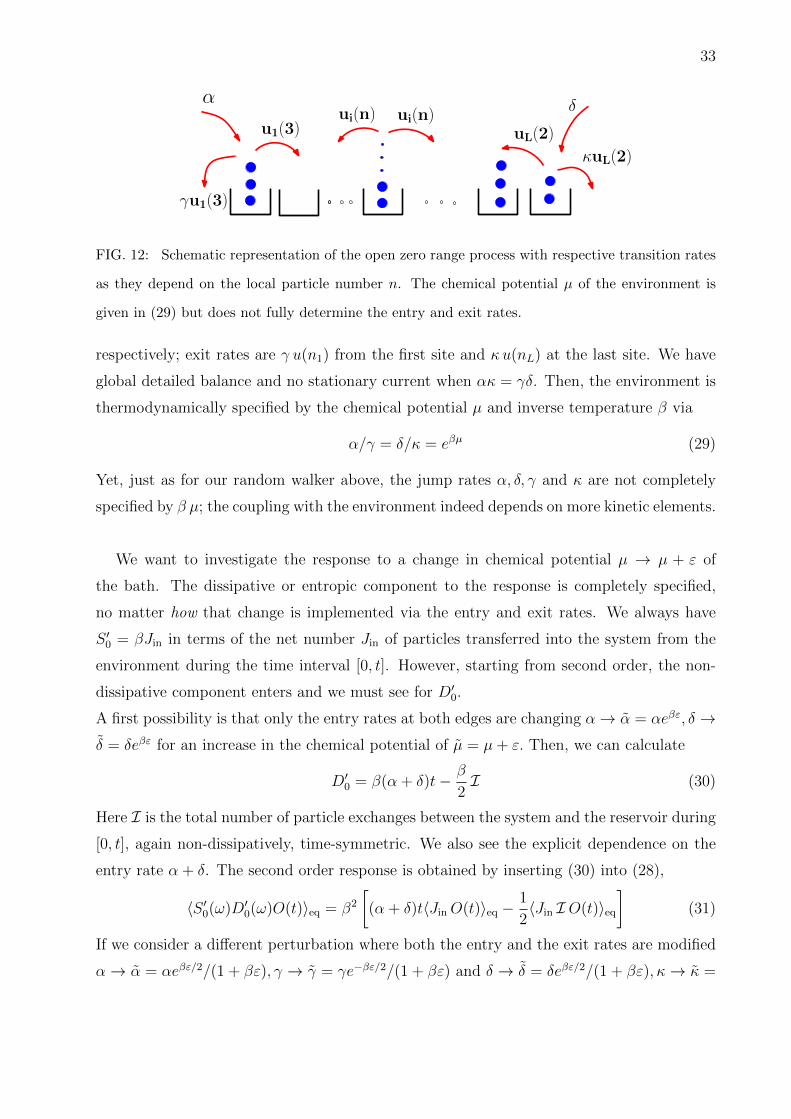
sion; see [48]. There are L sites and each is occupied with ni number of particles, see Fig. 12.
In the bulk a particle hops from site i to its right or left neighbor at rate u(ni). The bound-
ary sites are connected with particle reservoirs, their action being modeled via entrance and
exit rates at the left and right boundary sites i = 1 and i = L. Entry rates are α and δ
33
αui(n)ui(n)
δ
κuL(2)
u1(3)
γu1(3)
uL(2)
FIG. 12: Schematic representation of the open zero range process with respective transition rates
as they depend on the local particle number n. The chemical potential µ of the environment is
given in (29) but does not fully determine the entry and exit rates.
respectively; exit rates are γ u(n1) from the first site and κu(nL) at the last site. We have
global detailed balance and no stationary current when ακ = γδ. Then, the environment is
thermodynamically specified by the chemical potential µ and inverse temperature β via
α/γ = δ/κ = eβµ (29)
Yet, just as for our random walker above, the jump rates α, δ, γ and κ are not completely
specified by β µ; the coupling with the environment indeed depends on more kinetic elements.
We want to investigate the response to a change in chemical potential µ → µ + ε of
the bath. The dissipative or entropic component to the response is completely specified,
no matter how that change is implemented via the entry and exit rates. We always have
S ′0 = βJin in terms of the net number Jin of particles transferred into the system from the
environment during the time interval [0, t]. However, starting from second order, the non-
dissipative component enters and we must see for D′0.
A first possibility is that only the entry rates at both edges are changing α→ α = αeβε, δ →δ = δeβε for an increase in the chemical potential of µ = µ+ ε. Then, we can calculate
D′0 = β(α + δ)t− β
2I (30)
Here I is the total number of particle exchanges between the system and the reservoir during
[0, t], again non-dissipatively, time-symmetric. We also see the explicit dependence on the
entry rate α + δ. The second order response is obtained by inserting (30) into (28),
〈S ′0(ω)D′0(ω)O(t)〉eq = β2
[(α + δ)t〈JinO(t)〉eq −
1
2〈Jin I O(t)〉eq
](31)
If we consider a different perturbation where both the entry and the exit rates are modified
κe−βε/2/(1 + βε), while we still get the same shift in the chemical potential µ = µ + ε, the
frenetic part now has
D′0(ω) = β
[I − 1
2(α + δ)t− 3
2
∫ t
0
ds [γu(n1(s)) + κu(nL(s))]
]and
〈S ′0(ω)D′0(ω)O(t)〉 = β2
[〈JinI;O〉eq −
1
2(α + δ)t〈Jin;O(t)〉eq
−3
2
∫ t
0
ds 〈[γu(n1(s)) + κu(nL(s))] Jin;O(t)〉eq
]Here we see the explicit appearance of time-symmetric observables from second order re-
sponse on. The linear order response is exactly the same for the two types of perturbations,
indistinguishable because that is purely dissipative.
Experimental verification and use of the second order response as discussed here was done in
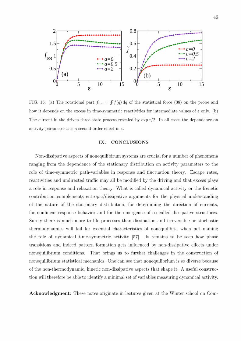
[47]; there the authors show that the non-dissipative contribution is measurable separately.
D. Breaking of local detailed balance
We have in all examples insisted on the assumption (1) of local detailed balance. That
is the modeling hypothesis so far for nonequilibrium (driven) systems. Here is however the
appropriate place to show the limitations of that assumption.
Suppose indeed we consider a probe in contact with a nonequilibrium system as the
ones we are discussing in these notes. The system interacts with the probe via a joint
interaction potential U(q, x) appearing in the total Hamiltonian. We denote by q the
probe’s position and x are the degrees of freedom of the medium. Clearly now the probe
will feel friction and noise from the nonequilibrium medium much in the same way as a
Brownian particle or a colloid suspended in an equilibrium Newtonian fluid. The relation
between friction and noise for the latter satisfies the Einstein relation, also called the
second fluctuation-dissipation relation. That in turn is responsible for the probe effective
evolution equation verifying local detailed balance as given for discrete processes in (1).
But that fails altogether for a probe in a nonequilibrium medium. The relation between
friction and noise is no longer the standard Einstein relation then, and the effective probe
dynamics will not satisfy local detailed balance, at least not with respect to the correct
physical entropy production. One can sometimes introduce effective parameters, like
an effective temperature to maintain an intuition but that seems more aligned with a
35
conservative approach as alluded at in the introduction of the present notes; see e.g. [49–51].
The idea in general is the following. The probe perturbs the stationary condition of the
medium by moving in it. The perturbation is felt as a change in the interaction potential
U(q, x)→ U(q, x) + (qs− q)V (x) with potential V (q, x) = ∂qU(q, x). As a consequence, the
medium responds following formulæ like (25). For example, suppose first that the medium is
in fact in equilibrium. Taking the amplitude hs = qs− qt we get a response on the expected
force 〈V (qt, xt)〉 as
K =
∫ t
0
ds (qs − qt)d
ds〈V (qt, xs)V (qt, xt)〉eq
by following formula (22). Partial integration in time yields the usual friction term as in a
generalized Langevin equation, with friction kernel related to the noise, having a covariance
in terms of force-force correlations. That would give the usual Einstein relation. But for a
nonequilibrium medium that responds to the probe motion we must replace (22) with (25)
and an additional term. the frenetic contribution indeed, will need to be added to K, while
the noise formula remains essentially unchanged. We refer to [49–51] for more details.
VI. FRENETIC BOUNDS TO DISSIPATION RATES
Thermalization or relaxation to equilibrium refers to the property of reduced systems or
variables of showing convergence in time to an equilibrium condition or value as set by the
constraints or conserved quantities in the larger system. The phrasing “reduced system”
either refers to a collection of macroscopic variables or empirical averages, e.g., the spatial
profile of some mass or energy density, or to some set of local observables e.g. belonging to
a subvolume. The idea is that many other degrees of freedom are left in contact with the
reduced system, are integrated out, and constitute a dynamical heat bath for the degrees
of freedom of the reduced system. That is also why the derivation of Brownian motion or
of more general stochastic evolutions in an appropriate coupling- and scaling-limit is an
essential ingredient in studies of thermalization. The literature on the subject is vast and
has been in the forefront of statistical physics up from the time of Boltzmann till today
where the relaxation of quantum systems remains a hot topic. A recurrent question there
has been how to unify the idea of a unitary or Hamiltonian dynamics with a possibly
dissipative dynamics for the reduced system. Often ergodic properties of the dynamics
have been called upon to make time-averages to coincide with some ensemble averages
36
etc. We will not discuss that issue here. As a more original contribution we emphasize
here that the structure of gradient flow as shown in macroscopic evolution equations is in
fact pointing to two separate aspects of relaxation, one which is entropic and dominates
close-to-equilibrium, and one which is frenetic and is crucial also far-from-equilibrium.
We use here the word “frenetic” to have a complement to “entropic” that emphasizes
the component of dynamical activity in relaxation processes. Secondly, we give a frame-
work, mainly dynamical fluctuation theory, in which both relaxation and stationarity can
be discussed and we indicate how to obtain from there frenetic bounds to the dissipation rate.
Gradient flow gives a differential-geometric characterization of certain dissipative relax-
ational processes for macroscopic systems. The heuristics is as follows. Suppose the reduced
system finds itself in some condition X, cf. the introduction I. The latter can refer to a
specific spatial profile of some density, in which case we really have a function ρ(r), r ∈ Vover some spatial domain V , or to the value of some macroscopic variable like the averaged
magnetization. The condition X need not be the one of equilibrium compatible with the
present constraints, and we ask in what direction the system will evolve from M . That
displacement is given by the change in X, or e.g. for a density profile ρ in terms of a cur-
rent j∗(ρ) which is one of many possible currents compatible with ρ and with any further
constraints on the system. The question is what determines that j∗ from ρ. The answer has
two parts, one thermodynamic and the other kinetic. The thermodynamic part refers to the
maximizing of the total entropy or the minimizing of some free energy. Gradient flow makes
the corresponding thermodynamic potential a Lyapunov function, monotone in time; that
is part of the H-theorem in the case of the Boltzmann equation for the thermalization of
dilute gases. So gradient flow moves in the direction of lower free energy or larger entropy
for the total universe, which is the usual Boltzmann picture of selecting that trajectory
which moves over macroscopic conditions that show ever larger phase space volumes to end
up finally in the equilibrium condition where the phase space volume is huge compared to
the initial ones. But that is not enough; moving out and in macroscopic conditions requires
certain amounts of accessibility and escape-ability – after all, there is a good reason that
relaxation times might be large. The point is that gradient flow is also following steepest
descent of the free energy. That steepest descent requires a distance or metric in the space
of macroscopic conditions; we must know the height lines of the free energy and where the
gradient is largest from the given M . That distance is not provided by the thermodynam-
37
ics but by the kinetics of the process. What enters for standard dissipative evolutions of
a density field ρ is the Onsager matrix of mobility or the diffusion constant, as function
of the condition ρ. The positivity of that Onsager matrix provides the local measure of
distance (the metric). All that is rather well-studied and known but less so in the nonlinear
regime where the condition is still far-from-equilibrium, and where the linearity between the
thermodynamic force (gradient of the potential) and the current does not need to hold.
Equilibrium
FIG. 13: The Boltzmann picture of relaxation to equilibrium, amended by the influence of “surface
effects” of the phase space region. Higher dynamical activity or escape rates on the reduced or
coarsed grained level of description decreases relaxation times.
Concerning the main point of these lectures indeed, it should be clear that non-dissipative
aspects should play a role also. Especially when starting well away from equilibrium,
visiting phase space regions with smaller volume, it appears not unreasonable to imagine
that also “surface” effects and not only volume effects will contribute to determine the
pathways to equilibrium. The exit and entrance rates from a macroscopic condition are not
determined by its volume (entropy) solely. That is the first heuristics behind suspecting
that time-symmetric quantities, like time-symmetric currents, will also appear essentially
outside equilibrium.
In fact, on the same level of discussion we can easily imagine that the interaction between
various components lead to effective kinetic constraints such that the relaxation becomes
very difficult. That “breaking of ergodicity” is studied in various models and sometimes is
referred to as glassy behavior or as many body localization [23]. The kinetic constraints are
basically involving non-dissipative aspects, having to do with trapping and caging effects in
phase space, which is just an abstraction of what happens in Fig. 10 (replacing there the
38
external field by thermodynamic forces and replacing the obstacles by either disorder in the
interaction or by specific many body effects).
Let us finally come also here to a more mathematical analysis. As often it pays to consider
the problem on space-time and to go on the level of fluctuation theory. That is the whole idea
of dynamical statistical ensembles, as we saw at work e.g. in Section V on response. Let us
however not start this time from more microscopic models but imagine how the macroscopic
equation for the relaxation to equilibrium, or more generally the displacements or currents
would be derived as function of the given macroscopic condition. We take therefore the view
that we have a family of possible trajectories ((ρs, js), s ∈ [0, t]) over a time-interval [0, t]
starting at time zero from the condition ρ0. The latter has also a certain probability which
is the subject of static fluctuations we touched in Sections III and III E. Indeed the ρs are
the possible density profiles on a certain level of description, so we would have e.g. ρs(x) for
the probability or density of particles at or in state x. The js are the corresponding currents
or displacements, and they are often constrained in the sense that only those trajectories
have non-zero probability for which
ρs +Djs = 0 (32)
where the operator D could be a (discrete or continuum) divergence in the case of a conserved
quantity, or also just unity for a reactive dynamics. Apart from such constraints as in (32)
all is possible; dynamical fluctuation theory is supposed to give us information about the
probabilities. These probabilities satisfy a law of large numbers in the limit where a scaling
factor N tends to infinity; N can indicate the size of the system or the number of particles
etc.; the precise origin and context for (32) can vary wildly. Fluctuations are corrections to
the law of large numbers and we assume therefore the asymptotic in N form,
Prob[(ρs, js), s ∈ [0, t]] = eNS[ρ0] exp[−N∫ t
0
L(ρs, js) ds] (33)
in terms of the static fluctuation rate S (called, nonequilibrium statistical entropy) and the
Lagrangian L ≥ 0. Via that scale N we can assume that there is a unique most typical
trajectory starting from ρ0. In other words we can find for every density (condition) ρ what
comes next by finding j∗ = j∗(ρ) as solution of the zero-cost flow:
L(ρ, j∗(ρ) = 0 (34)
39
All other possibilities are exponentially small in N ↑ ∞. If we are dealing with relaxation
processes, the solution j∗(ρ) will determine the macroscopic evolution equation by plugging it
in for the current in (32). One example where j∗(ρ) turns out to be linear in ρ is the Master
equation for Markov processes. In case we are dealing with a stationary nonequilibrium
process where the density is ρs = ρ∗ constant in time, we obtain through j∗(ρ∗) information
about the currents maintained in the system. Whatever the case we may in particular be
interested in the expected entropy production rate
σ(ρ) = σ(ρ, j∗(ρ)) (35)
corresponding to ρ. It is the dissipation rate, product of forces and fluxes, expressed as
function of the present system condition ρ. In the case of thermalization (relaxation to
equilibrium for a system open to energy exchanges at fixed environment temperature) (35)
is minus the rate of free energy decrease when in ρ. Lower bounds on σ(ρ) would give
information about relaxation times. In stationary nonequilibrium (density ρ∗) then σ∗ =
σ(ρ∗, j∗(ρ∗)) is the mean (stationary) entropy production rate. Then, lower bounds on σ∗
would give refinements on the second law like statement that σ∗ ≥ 0. To have a closer look
we can see to relate that entropy production rate to the dynamical fluctuations in (33).
The way (35) is related to the Lagrangian (and the dynamical fluctuations) is, as always,
via the condition of local detailed balance (1). More precisely, the entropy production rate
corresponding to a pair (ρ, j) of density and current, is the bilinear form that will be obtained
from the part in the Lagrangian that is antisymmetric under time-reversal:
σ(ρ, j) = L(ρ,−j)− L(ρ, j)
(We ignore here the presence of currents for odd degrees of motion, like momentum currents.)
The non-dissipative aspect of the Lagrangian (and dynamical fluctuations) resides in the
time-symmetric part, which we split up further in two parts:
L(ρ, j) + L(ρ,−j) = 2ψ(ρ, j) + 2L(ρ, 0)
For the interpretation we can look at specific models, but here is already some structure.
Suppose we have a density ρ and no current whatsoever, js = 0 for all times. Then, it must
be that ρs = ρ0 did not change, and the probability of such a trajectory is according to (33)
proportional with
exp−NtL(ρ0, 0)
40
In other words, L(ρ, 0) is the escape rate from ρ. Its inverse gives us the information of
the mean time the system resides in ρ, indeed invariant under time-reversal, but of course
depending on ρ and on all possible forces. Secondly, the ψ(ρ, j) is symmetric in j and
non-zero when j 6= 0. It is therefore the analogue of the activity parameters that we first
introduced under (2). It depends of course also on ρ and it gives the unoriented traffic in ρ
associated to j.
We are ready for the final line in the reasoning. If we look back at the zero-cost flow
(34)] with solution j∗(ρ), we obviously have that
1
2σ(ρ, j∗(ρ)) = ψ(ρ, j∗(ρ)) + L(ρ, 0) (36)
which says that the expected current j∗(ρ) given ρ is such that the dissipation rate (left-
hand side) equals the expected dynamical activity (right-hand side). We have here the
analogue of (26) but for macroscopic densities. The identity (36) has consequences in terms
of frenetic bounds for the expected entropy production rate, cf. [53]. Any lower bound
on the right-hand side of (36) provides a lower bound on the expected dissipation. Thus
we will get lower bounds on the mean entropy production rate which are symmetric in the
currents and non-dissipative, which leads to refinements of the second law version which
merely says that σ(ρ, j∗(ρ)) ≥ 0. It is important here to note that ψ(ρ, j) in convex in j
whenever L(ρ, j) is convex in j; that is because the time-antisymmetric part σ(ρ, j) is linear
in j to be compatible with local detailed balance. Because by construction ψ(ρ, 0) = 0 and
ψ(ρ, j) = ψ(ρ,−j) we then have that ψ(ρ, j) > 0 from the moment j 6= 0. So from the
moment there is a non-zero entropy production, we will have already the non-trivial bound
σ∗ ≥ ψ(ρ∗, j∗(ρ∗)) > 0. Finer frenetic bounds are discussed in [53].
VII. SYMMETRY BREAKING
We finally come to a major influence of non-dissipative aspects on nonequilibrium struc-
tures. To put it in contradictory terms and in line with the recent [54]: purely dissipative
trajectory ensembles are wrong because they do not allow dissipation. By a purely dissi-
pative trajectory ensemble we mean a probability distribution on trajectories, as in Section
V, where however the action with respect to equilibrium only contains the entropy flux. In
other words, looking back at (16) and (17), we would have an action A = λS proportional
to the entropy flux only, thus forgetting about the frenetic contribution D. Such ensembles
41
(which, disrepectfully, we will call mutilated) are often considered for modeling nonequilib-
rium in the spirit of maximum entropy or maximum caliber assumptions4. Yet, the point is
that these mutilated ensembles
Prob[ω] ∝ Probeq[ω] eλS(ω) (37)
often have additional symmetries which are unwanted. The main mathematical consequence
of (37) is that under time-reversal θ (defined in Section V A), Sθ = −S and hence,
Prob[θω] ∝ Probeq[ω] e−λS(ω)
by the time-reversal symmetry of the equilibrium ensemble. There may however still be
other involutions Γ leaving invariant the equilibrium ensemble for which S(Γω) = −S(ω)
and hence, for the mutilated ensemble (37),
Prob[Γθω] = Prob[ω]
(see equation (12) in [54] or equations (6)–(9) in [55]). Indeed, it is easy to imagine
for example how spatial reflection of ω inverts S(ω) in exactly the same way as does
time-reversal (and leaving the equilibrium reference invariant). It implies that we could
exchange time-reversal with spatial reflection, or more generally that we could induce
time-reversal by reversing the thermodynamic forces. Then, the dynamical ensemble of
a diffusion driven by some non-conservative field E would have a time-reversal which is
obtained by simply flipping E → −E . Now, since the stationary (single time) distribution of
the process is identical to the stationary distribution of the time-reversed process, we would
have that the stationary distribution is left invariant by flipping the field E → −E , which of
course is often very wrong. But even forgetting about that last point5, all expectations of
time-symmetric observables would be invariant under E → −E , 〈ΓO〉 = 〈O〉 when θO = O,
and all expectations of time-antisymmetric observables would be antisymmetric under
E → −E , 〈ΓO〉 = −〈O〉 when θO = −O. For example, from the last equality, for an energy
current J we would have 〈ΓJ〉 = −〈J〉 but often ΓJ = J so that we would need to conclude
4 More positively, such maximum entropy principles can teach us what observables or quantities are missing
in the variational formulation. Here for example we will learn that there is more than the values of currents
or of entropy flux alone that characterize the nonequilibrium ensemble.5 After all, the idea of stationary distribution has lost most of its meaning now since the trajectories
distributed by (37) are not associated to a Markovian time-evolution.
42
that 〈J〉 = 0, no dissipation!
In other words, such nonequilibrium ensemble (37), lacking non-dissipative terms in the
action, would not be able to break certain symmetries. That point was first stressed in
the theory of [55]. Also an example was given there of a viscous fluid under influence of
a pressure difference in some tube. In the laminar flow regime (left part of Fig. 14) we
indeed cannot distinguish between reversal of time and reversal of pressure difference. Yet,
at higher pressure differences (right part of Fig. 14), when things get really nonequilibrium,
the laminar pattern breaks up, the flow becomes turbulent and time-reversal definitely differs
from field-reversal. Another and older example where such symmetry breaking is essential is
found in [56]. There a turbulent boundary layer flow is considered over a smooth symmetric
hump; see Fig. 14. For the ensemble (37) there would never be a possibility to break that
ε� 1 ε
FIG. 14: Flow of particles driven by a field E . Left: for small driving we get a laminar flow without
symmetry breaking. Time-reversal equals field reversal. Right: For appreciable field strength
turbulent flow develops and the spatial symmetry gets broken essentially by the non-dissipative
frenetic contribution in the action, which is absent in the ensemble (37).
symmetry. Yet, true nonequilibrium does create a weak symmetry breaking, indeed visible
for aeolian sand transport and dune formation.
Note still that the ensemble (37) is compatible with the Kubo formula and linear response
around equilibrium, exactly for the (same) reasons that lead to (20) and (23). Moreover, so
called fluctuation symmetries [42] are trivially true. Yet, they lack the non-dissipative ele-
ments that are essential for creating interesting nonequilibria. To maintain the paradoxical
phrasing, interesting dissipative structures crucially depend on non-dissipative aspects.
43
VIII. FRENOMETRY
The question arises how non-dissipative aspects can be isolated and/or measured. Is
there something like measuring excesses in dynamical activity, as we encounter for example
in the frenetic contribution to response functions? Obviously all effects discussed in these
notes can be inverted: whenever we understand how activity parameters have an influence,
then we can also start from that theory to learn about these activity parameters from the
observed facts. Let us first see what that means for thermodynamic potentials.
Entropy is of course not directly measured — it is obtained via measurements of heat
capacity or from heat measurements more generally. Similarly, free energies are measured
from isothermal work, as we remember from the following type of calculation. Suppose that
the states x of a system are coupled to some real variable q, say the position of a probe, via
the interaction energies E(x, q). The mechanical force on q is −∇qE(x, q). For a quasi-static
probe we can take the statistical average over the equilibrium distribution,
feq(q) =∑x
1
Zqe−βE(x,q) (−∇qE(x, q)) =
1
β∇q logZq = −∇qF(q)
In other words, the statistical force is gradient with potential given by the free energy
(now depending on q). It is then clear how reversible isothermal transformations will have
changes in free energy given by the work done on the probe.
The idea for measuring non-dissipative aspects can proceed similarly.
In general we have that statistical forces out-of-equilibrium are given by
f(q) =∑x
ρq(x) (−∇qE(x, q))
where ρq(x) is the stationary distribution of a nonequilibrium medium with degrees of free-
dom x, which is coupled via interaction energy E(x, q) to a quasi-static probe with position
q. Clearly, as we have seen throughout these notes, the distribution ρq(x) will contain non-
dissipative aspects. Therefore, measuring the work done by the statistical force f(q) on a
probe will reveal aspects of dynamical activity, changes in escape rates or in time-symmetric
parts of reactivities. That is the general idea, but of course we need to implement it in spe-
cific situations. Paradoxically, as the system dissipates more, more non-dissipative features
become visible.
44
A. Reactivities, escape rates
Look again at the situation depicted in Fig. 10.
Suppose you would like to measure the dependence of the escape rate ψ(W,x) on the external
driving field. What we will do is to couple the walker to a probe with position q for example
as a load connected to the walker via a spring,
E(x, q) =λ
2(x− q)2
The stationary distribution of the driven particles for high field W can be approximated by
dividing an elementary interval length L, say between two major obstacles, in three different
states, one for the walker being directly behind the obstacle, another for being in the middle
of the interval and yet a third state for being in front of an obstacle; see Fig. 10. We then
write ρq(x) ' z/ψ(W,x), independent of probe position q for very small λ. That is similar
to what we saw already in Fig. 2, how the reactivities determine the stationary distribution.
The statistical force on the probe (load) is then approximated by
f(q;W,λ) = z λ
∫ L
0
(q − x)1
ψ(W,x)dx
telling us about the escape rate ψ(W,x). When we find the position of the probe where
the statistical force is zero, f(q∗;W ) = 0, we will get information about the escape rate
profile. For example, if we take ψ(W,x) = e−aWx, x ∈ [0, L], then the stationary position
of the probe will be at q∗ = L − 1/(aW ) + . . . for large W , from which we would find
the slope coefficient a. The probe will find itself in a harmonic well for effective potential
λ(q − L+ 1/(aW ))2/2.
B. Non-gradient aspects are non-dissipative
Another tool to derive information about non-dissipative aspects of a nonequilibrium
medium is to look at the rotational part in the statistical force induced on a probe. In
fact, the very presence of a rotational component to the statistical force is produced by the
simultaneous appearance of excess entropy flux and excess dynamical activity when the
medium relaxes to a new stationary condition after displacing the probe.
The simplest example of how the statistical force can pick up the dependence of reactiv-
ities on the driving goes as follows; see also [52].
45
We follow a probe on the unit circle, q ∈ S1, in contact with a thermal bath at inverse
temperature β = 1, modeled via the overdamped Langevin dynamics
γq = − ∂
∂qE(x, q) +
√2γ ξt
for ξt standard white noise, γ is the damping coefficient and there is an interaction with an
‘internal’ degree of freedom x = −1, 0, 1 with potential
E(x, q) = x sin q + 2x2 cos q
The x is the fast degree of freedom, driven with transition rates
kq(x, x′) = e−β2
[E(x′,q)−E(x,q)] φ(x, x′) e12s(x,x′)
The drive is uniform, with s(−1, 1) = s(1, 0) = s(0,−1) = ε but we assume that also the
symmetric activity parameters φ(x, x′) = φ(x′, x) are affected via φ(−1, 1) = φ(1,−1) =
φ0(1 + a|ε|) for some a ≥ 0, while φ(0,±1) = φ(±1, 0) = 1. Detailed balance is achieved
at ε = 0, where φ0 picks up the relative importance of the dynamical activity over the
transitions 1↔ −1.
The statistical force on the probe is
f(q) = −〈x〉q cos q + 2〈x2〉q sin q (38)
and can be calculated exactly. For driving ε 6= 0 there are no symmetries forbidding
the probe to have net motion (Curie’s principle) and hence to show a systematic current
round the circle. The rotational part of the force frot =∮f(q) dq is plotted versus ε in
Fig. 15(a). Observe that the rotational force depends on the coefficient a, and hence picks
up information about that non-dissipative part φ(x, x′) in the reaction rates. In fact, we
see clearly, take a = 1/2, that the rotational force is maximal for an intermediate ε ' 4.
For larger a ≥ 0 we get less rotational force on the probe, because the medium gets more
jammed, in fact similarly again to what happens in Fig. 2(b) for large b.
Fig. 15(b), where we see the current in the medium process, must be compared with
Fig. 15(a): there is no simple relation between the rotational power in the probe and the
entropy production in the medium. Non-dissipative players decide when well away from
equilibrium (ε = 0). We see that in the dependence on the parameter a for the change in
reactivity with ε but the time-symmetric part in the action is of course also changing with
ε.
46
0 5 10 15ε
0
0.5
1
1.5
2
frot a=0
a=0.5a=2
0 5 10 15ε
0
0.2
0.4
0.6
0.8
J a=0a=0.5a=2
~
(a) (b)
FIG. 15: (a) The rotational part frot =∮f(q) dq of the statistical force (38) on the probe and
how it depends on the excess in time-symmetric reactivities for intermediate values of ε only. (b)
The current in the driven three-state process rescaled by exp ε/2. In all cases the dependence on
activity parameter a is a second-order effect in ε.
IX. CONCLUSIONS
Non-dissipative aspects of nonequilibirum systems are crucial for a number of phenomena
ranging from the dependence of the stationary distribution on activity parameters to the
role of time-symmetric path-variables in response and fluctuation theory. Escape rates,
reactivities and undirected traffic may all be modified by the driving and that excess plays
a role in response and relaxation theory. What is called dynamical activity or the frenetic
contribution complements entropic/dissipative arguments for the physical understanding
of the nature of the stationary distribution, for determining the direction of currents,
for nonlinear response behavior and for the emergence of so called dissipative structures.
Surely there is much more to life processes than dissipation and irreversible or stochastic
thermodynamics will fail for essential characteristics of nonequilibria when not naming
the role of dynamical time-symmetric activity [57]. It remains to be seen how phase
transitions and indeed pattern formation gets influenced by non-dissipative effects under
nonequilibrium conditions. That brings us to further challenges in the construction of
nonequilibrium statistical mechanics. One can see that nonequilibrium is so diverse because
of the non-thermodynamic, kinetic non-dissipative aspects that shape it. A useful construc-
tion will therefore be able to identify a minimal set of variables measuring dynamical activity.
Acknowledgment: These notes originate in lectures given at the Winter school on Com-
47
plexity at the TU Eindhoven in December 2015. Special thanks to Mark Peletier for the
encouragement to start writing them down. I am also very indebted to my collaborators of
which the joint papers appear below in the references.
[1] S. De Groot, and P. O. Mazur, Non-Equilibrium Thermodynamics, Dover Pub. (1962).
[2] C. Maes, What decides the direction of a current? Mathematics and Mechanics of Complex
Systems 3, 275–295 (2016).
[3] S. Katz, J.L. Lebowitz, and H. Spohn, Stationary nonequilibrium states for stochastic lattice
gas models of ionic superconductors, J. Stat. Phys. 34, 497 (1984).
[4] C. Maes and K. Netocny, Time-reversal and Entropy. J. Stat. Phys. 110, 269 (2003).
[5] T. Harada and S.-I. Sasa, Equality connecting energy dissipation with violation of fluctuation-
response relation. Phys. Rev. Lett. 95, 130602 (2005).
[6] B. Derrida, Non-equilibrium steady states: fluctuations and large deviations of the density
and of the current. J. Stat. Mech. P07023 (2007).
[7] H. Tasaki, Two theorems that relate discrete stochastic processes to microscopic mechanics.
arXiv:0706.1032v1.
[8] http://www.nil.wustl.edu/labs/corbetta/research spont activity.html. Last visited
1 June 2017.
[9] F. Michler, H. van Hees, D.D. Dietrich, S. Leupold and C. Greiner, Non-equilibrium photon
production arising from the chiral mass shift. arXiv:1304.4093 [nucl-th].
[10] C. Maes and K. Netocny, Minimum entropy production principle. Scholarpedia 8(7), 9664
(2013).
[11] C. Maes and W. O’Kelly de Galway, On the kinetics that moves Myosin V. Physica A: Sta-
tistical Mechanics and its Applications 436, 678–685 (2015).
[12] W. De Roeck and C. Maes, Symmetries of the ratchet current. Phys. Rev. E 76, 051117 (2007).
[13] P. Baerts, U. Basu, C. Maes and S. Safaverdi, The frenetic origin of negative differential
response, Phys. Rev. E 88, 052109 (2013).
[14] R.K.P. Zia, E. L. Præstgaard, and O.G. Mouritsen, Getting more from pushing less: Negative
specific heat and conductivity in nonequilibrium steady states. Am. J. Phys. 70, 384 (2002).
[15] U. Basu and C. Maes, Mobility transition in a dynamic environment. J. Phys. A: Math. Theor.
48
47, 255003 (2014).
[16] O. Benichou, P. Illien, G. Oshanin, A. Sarracino, R. Voituriez, Microscopic theory for negative
differential mobility in crowded environments. Phys. Rev. Lett. 113, 268002 (2014).
[17] M. Baiesi, A. Stella, and C. Vanderzande, Role of trapping and crowding as sources of negative