Non-line-of-sight imaging using atime-gated single photon avalanche diode

Mauro Buttafava,1,5 Jessica Zeman,2,5 Alberto Tosi,1 KevinEliceiri,2,3,4 and Andreas Velten2,3,4,∗

1 Dipartimento di Elettronica, Informazione e Bioingegneria, Politecnico di Milano, Milano,Italy

2 Laboratory for Optical and Computational Instrumentation, University of Wisconsin,Madison, WI, USA

3 Morgridge Institute for Research, Madison, WI, USA4 Wisconsin Institute for Discovery, Madison, WI, USA

5 These authors contributed equally to this work∗velten@wisc.edu

Abstract: By using time-of-flight information encoded in multiplyscattered light, it is possible to reconstruct images of objects hidden fromthe camera’s direct line of sight. Here, we present a non-line-of-sightimaging system that uses a single-pixel, single-photon avalanche diode(SPAD) to collect time-of-flight information. Compared to earlier sys-tems, this modification provides significant improvements in terms ofpower requirements, form factor, cost, and reconstruction time, whilemaintaining a comparable time resolution. The potential for furthersize and cost reduction of this technology make this system a good basefor developing a practical system that can be used in real world applications.

References and links1. T. Ralston, G. Charvat, and J. Peabody, “Real-time through-wall imaging using an ultrawideband multiple-

input multiple-output (MIMO) phased array radar system,” in Proceedings of IEEE International Symposiumon Phased Array Systems and Technology (IEEE, 2010), pp. 551–558.

2. B. Chakraborty, Y. Li, J. Zhang, T. Trueblood, A. Papandreou-Suppappola, and D. Morrell, “Multipath exploita-tion with adaptive waveform design for tracking in urban terrain,” in Proceedings of IEEE International Confer-ence on Acoustics Speech and Signal Processing (IEEE, 2010), pp. 3894–3897.

3. A. Sume, M. Gustafsson, M. Herberthson, A. Janis, S. Nilsson, J. Rahm, and A. Orbom, “Radar Detection ofMoving Targets Behind Corners,” IEEE Trans. Geosci. Remote Sens. 49, 2259–2267 (2011).

4. P. Sen, B. Chen, G. Garg, S. R. Marschner, M. Horowitz, M. Levoy, and H. P. A. Lensch, “Dual Photography,”ACM Trans. Graph. 24, 745–755 (2005).

5. E. Repasi, P. Lutzmann, O. Steinvall, M. Elmqvist, B. Ghler, and G. Anstett, “Advanced short-wavelength infraredrange-gated imaging for ground applications in monostatic and bistatic configurations,” Appl. Opt. 48, 5956–5969 (2009).

6. J. C. Hebden, R. A. Kruger, and K. S. Wong, “Time resolved imaging through a highly scattering medium,” Appl.Opt. 30, 788–794 (1991).

7. S. Gokturk, H. Yalcin, and C. Bamji, “A Time-Of-Flight Depth Sensor - System Description, Issues and Solu-tions,” in Proceedings of Conference on Computer Vision and Pattern Recognition Workshop (IEEE, 2004), pp.35–35.

8. N. Abramson, “Light-in-flight recording by holography,” Opt. Lett. 3, 121–123 (1978).9. A. Velten, D. Wu, A. Jarabo, B. Masia, C. Barsi, C. Joshi, E. Lawson, M. Bawendi, D. Gutierrez, and R. Raskar,

“Femto-photography: Capturing and Visualizing the Propagation of Light,” ACM Trans. Graph. 32, 44 (2013).

10. A. Kadambi, R. Whyte, A. Bhandari, L. Streeter, C. Barsi, A. Dorrington, and R. Raskar, “Coded Time of FlightCameras: Sparse Deconvolution to Address Multipath Interference and Recover Time Profiles,” ACM Trans.Graph. 32, 167 (2013).

11. F. Heide, M. B. Hullin, J. Gregson, and W. Heidrich, “Low-budget Transient Imaging Using Photonic MixerDevices,” ACM Trans. Graph. 32, 45 (2013).

12. M. O’Toole, F. Heide, L. Xiao, M. B. Hullin, W. Heidrich, and K. N. Kutulakos, “Temporal Frequency Probingfor 5d Transient Analysis of Global Light Transport,” ACM Trans. Graph. 33, 87 (2014).

13. F. Heide, L. Xiao, W. Heidrich, and M. B. Hullin, “Diffuse Mirrors: 3d Reconstruction from Diffuse Indirect Il-lumination Using Inexpensive Time-of-Flight Sensors,” in Proceedings of IEEE Conference on Computer Visionand Pattern Recognition (IEEE, 2014), pp. 3222–3229.

14. G. Gariepy, N. Krstaji, R. Henderson, C. Li, R. R. Thomson, G. S. Buller, B. Heshmat, R. Raskar, J. Leach, andD. Faccio, “Single-photon sensitive light-in-flight imaging,” Nat. Commun. 6, 6021 (2015).

15. A. Kirmani, T. Hutchison, J. Davis, and R. Raskar, “Looking Around the Corner using Ultrafast Transient Imag-ing,” Int. J. Comput. Vision 95, 13–28 (2011).

16. A. Velten, T. Willwacher, O. Gupta, A. Veeraraghavan, M. G. Bawendi, and R. Raskar, “Recovering three-dimensional shape around a corner using ultrafast time-of-flight imaging,” Nat. Commun. 3, 745 (2012).

17. O. Gupta, T. Willwacher, A. Velten, A. Veeraraghavan, and R. Raskar, “Reconstruction of hidden 3d shapes usingdiffuse reflections,” Opt. Express 20, 19096–19108 (2012).

18. M. Laurenzis and A. Velten, “Nonline-of-sight laser gated viewing of scattered photons,” Opt. Eng. 53, 023102–023102 (2014).

19. F. Zappa, S. Tisa, A. Tosi, and S. Cova, “Principles and features of single-photon avalanche diode arrays,” SensorsActuat. A: Phys. 140, 103–112 (2007).

20. G. Gariepy, F. Tonolini, R. Henderson, J. Leach, and D. Faccio, “Tracking hidden objects with a single-photoncamera,” http://arxiv.org/abs/1503.01699 .

21. F. Villa, D. Bronzi, Y. Zou, C. Scarcella, G. Boso, S. Tisa, A. Tosi, F. Zappa, D. Durini, S. Weyers, U. Paschen,and W. Brockherde, “CMOS SPADs with up to 500 m diameter and 55% detection efficiency at 420 nm,” J. Mod.Optic. 61, 102–115 (2014).

22. M. Buttafava, G. Boso, A. Ruggeri, A. D. Mora, and A. Tosi, “Time-gated single-photon detection module with110 ps transition time and up to 80 MHz repetition rate,” Rev. Sci. Instrum. 85, 083114 (2014).

23. E. F. Pettersen, T. D. Goddard, C. C. Huang, G. S. Couch, D. M. Greenblatt, E. C. Meng, and T. E. Ferrin, “UCSFChimeraA visualization system for exploratory research and analysis,” J. Comput. Chem. 25, 1605–1612 (2004).

24. A. Rochas, M. Gosch, A. Serov, P. Besse, R. Popovic, T. Lasser, and R. Rigler, “First fully integrated 2-D arrayof single-photon detectors in standard CMOS technology,” IEEE Photon. Technol. Lett. 15, 963–965 (2003).

25. A. Ruggeri, P. Ciccarella, F. Villa, F. Zappa, and A. Tosi, “Integrated Circuit for Subnanosecond Gating ofInGaAs/InP SPAD,” IEEE J. Quantum Electron. 51, 4500107 (2015).

26. B. Markovic, S. Tisa, F. Villa, A. Tosi, and F. Zappa, “A High-Linearity, 17 ps Precision Time-to-Digital Con-verter Based on a Single-Stage Vernier Delay Loop Fine Interpolation,” IEEE Trans. Circuits and Syst. 60, 557–569 (2013).

27. Y. Barkana and M. Belkin, “Laser Eye Injuries,” Surv. Ophthalmol. 44, 459–478 (2000).28. J. Zhang, R. Thew, C. Barreiro, and H. Zbinden, “Practical fast gate rate InGaAs/InP single-photon avalanche

photodiodes,” Appl. Phys. Lett. 95, 091103 (2009).

1. Introduction

One of the motivations for developing non-line-of-sight imaging is to remotely view areas thatare difficult or dangerous to access. Potential applications of this technology include monitoringhazardous industrial environments, improving spatial awareness in robotic surgery, and search-ing disaster zones for survivors. There is also a desire to use it in security applications, vehiclenavigation and for remote exploration via air and spaceborne imaging systems. The practicalityof employing these systems outside of the laboratory is currently limited by their cost, lack ofportability, time resolution, and signal-to-noise ratio.

Non-line-of-sight imaging has been demonstrated using both radio and visible wavelengths.At radio wavelengths, systems have been developed to create low resolution images throughwalls [1], around corners using specular reflections [2], and to detect motion around a cor-ner [3]. These systems typically require large apertures, especially when the imaging system isfar from the scene to be imaged. Methods of doing non-line-of sight imaging at visible wave-lengths include using a coded controllable light source, such as a projector, to illuminate hiddenobjects [4] or using specular reflections in a window pane [5]. Photon time-of-flight, which is

typically used for ranging in imaging LIDAR or gated viewing systems [6, 7], can also be ap-plied to multiply reflected light to image beyond the direct line of sight.

One of the first techniques used to create time-of-flight videos or transient images was holo-graphic light-in-flight imaging [8]. This method only captures direct, first bounce light and can-not be used for the light transport analysis of light undergoing multiple reflections. Transientimaging of multiply reflected incoherent light has been demonstrated using a streak camera [9],inexpensive photonic mixer devices [10–13], and Single-Photon Avalanche Diode (SPAD) ar-rays [14].

These devices are also able to capture the light transport information encoded in multi-ply scattered light, which can be used to reconstruct images of scenes beyond the direct lineof sight [15]. A streak camera based system was one of the first to demonstrate this tech-nique [16, 17]. This system provided time resolutions down to 2 picoseconds and a lateralspatial resolution of approximately 1 cm in the reconstruction. The size, price (approximately$150,000), and fragility of the streak camera limit the applications of such a system.

In attempts to make these systems more practical, interest has turned to using time modulatedsource and detection devices such as photonic mixer devices (PMDs) [13]. These devicesare compact and inexpensive (less than $500), but are limited to a time resolution of severalnanoseconds or a spatial resolution of approximately 3 meters. It is possible to reconstructsmaller scenes with the help of regularization, but this requires the incorporation of additionalassumptions about the scene, such as the absence of volumetric scattering [13].

Another method of collecting time-of-flight information is to use a microchip laser in com-bination with a gated intensified Charge-Coupled Device (iCCD) camera [18]. This system isportable and has a time resolution of several hundred picoseconds. While less expensive than astreak camera based system, an iCCD camera, at $80,000 is still above the price range of massmarket applications. It also has a low photon count rate, making it less ideal for this type ofwork.

Our system uses a single SPAD detector. SPADs are solid-state photodetectors that are ableto collect extremely fast and weak light signals, down to the single photon level [19]. A siliconSPAD is essentially a p-n junction, reverse biased above its breakdown voltage. A single photo-generated charge carrier absorbed in this junction can trigger a self-sustaining avalanche thatcan be detected by an external readout circuit. SPADs can be gated by modulating the biasvoltage a few volts above or below the breakdown value to filter incoming photons. Recently,non-line-of-sight tracking of the position of a single object in an empty space using a 32 by 32non-gated SPAD array was demonstrated [20].

We use a single gated SPAD detector along with a scanned laser to produce full reconstruc-tions of complex scenes. We demonstrate reconstruction with approximately 10 cm resolutionusing normal surface materials at an average illumination power of 50 mW.

2. Experimental setup

The major components of our system include a laser light source, a SPAD detector, a time-correlated single photon counting (TCSPC) module, and the hidden scene to be imaged.Fig. 1(a) shows the light path through our experimental setup.

The light source is an Amplitude Systems Mikan Laser, generating 250 fs long pulses witha repetition rate of 55 MHz and wavelength of 1030 nm. This wavelength is doubled to createa pulse train at 515 nm with an average power of 50 mW. This is an order of magnitude lowerthan the laser power used by Velten et al. [16]. The pulse train is directed towards one of theside walls of the laboratory using a pair of galvanometer-actuated mirrors following the patternshown in Fig. 1(b).

Returning photons are collected using a time-gated SPAD with a 20 µm diameter active-

Lase

r

SPAD

S

D

s

d

r1

r2

r3

r4

Camera

Lab

Wal

l

Object

(a) (b)

Fig. 1. (a) shows the light path through our system. The laser pulse is directed towards thewall by a set of galvanometer mirrors at point S. The light strikes the wall at point s viar1. Some of the light is reflected back to the detector (first bounce light) and the rest isscattered throughout the scene. A small amount of light goes towards the object via r2, isreflected back to the wall via r3, strikes the wall at point d, and is detected at D. The cameratakes pictures of the laser spots on the wall. Data is collected for different positions s onthe wall, following the laser scanning pattern shown in (b).

area [21]. This detector is made using a standard 0.35 µm Complementary Metal Oxide Semi-conductor (CMOS) technology. With a 7 V excess-bias voltage, it exhibits a photon detectionefficiency of up to 35% at 515 nm with less than 10 dark counts per second at 273 K. Theafterpulsing probability is lower than 1% with a 50 ns hold-off time. The timing jitter on thisdetector is a key parameter in the present work. In our case, it is better than 30 ps full widthat half maximum (FWHM), which corresponds to a traveled path length of about 1 cm at thespeed of light.

The time-gating feature of the SPAD allows us to disable the detector during the arrival of thefirst bounce light (indicated by the dashed arrow in Fig. 1(a)), which would otherwise blind thedetector from subsequent bounces. Our SPAD module achieves ON and OFF transition timesdown to 110 ps, at repetition rates up to 80 MHz and has an adjustable ON-time between 2 nsand 500 ns [22]. In our experiments, the detector ON-time window has a duration of 9.5 ns.This time was chosen as it provides the best compromise between first bounce rejection andextension of the reconstruction volume.

This detector is focused on a single spot covering a 1 cm2 area of the wall, using a 1” diameterlens with a 1” focal length. The detector field of view is not changed during the experiment.The detector is protected by an interference filter with a peak transmission at 515 nm and aFWHM bandwidth of 10 nm.

A Time Correlated Single Photon Counting (TCSPC) unit (PicoQuant HydraHarp) is used toproduce a histogram of the photon counts versus the number of time bins after the illuminationpulse. This system uses the trigger output of the laser as the time-base. An example of thehistogram produced by the TCSPC unit is shown in Fig. 2.

The pattern we use results in 185 datasets or time series. For an exposure time of 1 or 10seconds, the total capture time is about 5 or 32 minutes respectively.

The objects placed in the scene include two white patches of different sizes, and a 38 by41 cm letter T made of white paper. These objects are placed so they span the entire availablereconstruction volume, as defined by the repetition rate of the laser. In our case, this is approx-imately a quarter of a sphere with a radius of 1.5 meters since we only reconstruct above theplane of the optical table in front of the wall. We are not able to detect objects outside this areabecause their reflected light is blocked by the gate closing to prevent the detection of the next

0 2000 4000 6000 80000

10

20

30

40

Time [ps]

Cou

nts

(a) (b)

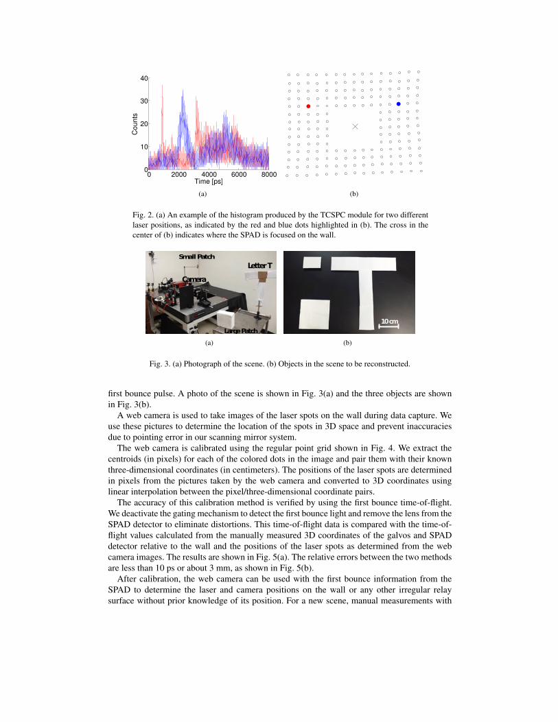
Fig. 2. (a) An example of the histogram produced by the TCSPC module for two differentlaser positions, as indicated by the red and blue dots highlighted in (b). The cross in thecenter of (b) indicates where the SPAD is focused on the wall.

Letter TSmall Patch

Camera

Large Patch

(a)

10 cm

(b)

Fig. 3. (a) Photograph of the scene. (b) Objects in the scene to be reconstructed.

first bounce pulse. A photo of the scene is shown in Fig. 3(a) and the three objects are shownin Fig. 3(b).

A web camera is used to take images of the laser spots on the wall during data capture. Weuse these pictures to determine the location of the spots in 3D space and prevent inaccuraciesdue to pointing error in our scanning mirror system.

The web camera is calibrated using the regular point grid shown in Fig. 4. We extract thecentroids (in pixels) for each of the colored dots in the image and pair them with their knownthree-dimensional coordinates (in centimeters). The positions of the laser spots are determinedin pixels from the pictures taken by the web camera and converted to 3D coordinates usinglinear interpolation between the pixel/three-dimensional coordinate pairs.

The accuracy of this calibration method is verified by using the first bounce time-of-flight.We deactivate the gating mechanism to detect the first bounce light and remove the lens from theSPAD detector to eliminate distortions. This time-of-flight data is compared with the time-of-flight values calculated from the manually measured 3D coordinates of the galvos and SPADdetector relative to the wall and the positions of the laser spots as determined from the webcamera images. The results are shown in Fig. 5(a). The relative errors between the two methodsare less than 10 ps or about 3 mm, as shown in Fig. 5(b).

After calibration, the web camera can be used with the first bounce information from theSPAD to determine the laser and camera positions on the wall or any other irregular relaysurface without prior knowledge of its position. For a new scene, manual measurements with

Fig. 4. The image of the grid used for web camera calibration. The dots are 5 cm apart andorigin of the 3D coordinates system is marked by the black cross in the lower right corner.

respect to the relay surface would no longer be necessary.

Tim

e B

in [

ps]

Laser Position

(a)

Tim

e B

in [

ps]

Laser Position

(b)

Fig. 5. Spacing between time bins is 1 ps. (a) Comparison of the measured time-of-flightin time bins(blue .) with the time-of-flight calculated from the 3D coordinates(magenta *).(b) The differences between the the measured and calculated first bounce time-of-flight.

3. Reconstruction method

For image reconstruction we use a modified version of the backprojection algorithm presentedby Velten et al. [16]. While other methods have shown superior resolution and reconstructionquality, such as the convex optimization algorithm used by Heide et al. [13], the size of theprojection matrix that would be required for our reconstruction makes this method unfeasible.Since the size of this matrix is determined by the product of the number of laser positions, cam-era positions, time points, and voxels in the reconstruction volume, the size of our projectionmatrix would be on the order of 2 terabytes. A filtered backprojection also does not requireassumptions about the hidden scene geometry and can be used without regularization. Morecomplex reconstruction methods can also make it difficult to separate hardware and softwarebased artifacts.

Our algorithm uses the number of photons counted per time bin, the photon time of arrivalt, the coordinates of the laser spot on the wall xi and yi, and the coordinates of the spot on thewall observed by the detector xo and yo to determine the location and geometry of the hiddenobject.

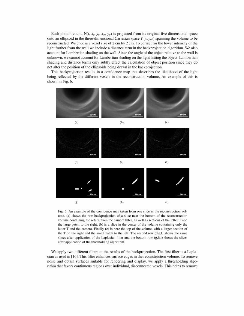
Each photon count, N(t, xi, yi, xo, yo) is projected from its original five dimensional spaceonto an ellipsoid in the three-dimensional Cartesian space V (x,y,z) spanning the volume to bereconstructed. We choose a voxel size of 2 cm by 2 cm. To correct for the lower intensity of thelight further from the wall we include a distance term in the backprojection algorithm. We alsoaccount for Lambertian shading on the wall. Since the angle of the object relative to the wall isunknown, we cannot account for Lambertian shading on the light hitting the object. Lambertianshading and distance terms only subtly effect the calculation of object position since they donot alter the position of the ellipsoids being drawn in the backprojection.

This backprojection results in a confidence map that describes the likelihood of the lightbeing reflected by the different voxels in the reconstruction volume. An example of this isshown in Fig. 6.

50cm

(a)

50cm

(b)

50cm

(c)

50cm

(d)

50cm

(e)

50cm

(f)

50cm

(g)

50cm

(h)

50cm

(i)

Fig. 6. An example of the confidence map taken from one slice in the reconstruction vol-ume. (a) shows the raw backprojection of a slice near the bottom of the reconstructionvolume containing the return from the camera filter, as well as sections of the letter T andthe large patch to the right. (b) is a slice in the center of the volume containing only theletter T and the camera. Finally (c) is near the top of the volume with a larger section ofthe T on the right and the small patch to the left. The second row (d,e,f) shows the sameslices after application of the Laplacian filter and the bottom row (g,h,i) shows the slicesafter application of the thresholding algorithm.

We apply two different filters to the results of the backprojection. The first filter is a Lapla-cian as used in [16]. This filter enhances surface edges in the reconstruction volume. To removenoise and obtain surfaces suitable for rendering and display, we apply a thresholding algo-rithm that favors continuous regions over individual, disconnected voxels. This helps to remove

some of the noise that would be present in the 3D reconstruction. Removing the distance andLambertian shading terms does not negatively impact the results of the thresholding algorithm,indicating that the decreased intensity due to those factors is not significant in our case. In-cluding Lambertian shading, actually tends to amplify noise at the edges of the reconstructionvolume and often leads to subjectively inferior reconstruction results. The backprojected ellip-soids have a thickness that is determined by the time resolution and by the size of the laser spotand the size of the area where the SPAD is focused on the wall, as illustrated by s and d respec-tively in Fig. 1(a). Broadening of the ellipsoid due to time resolution is implicitly included inthe backprojection since the sampling rate in the data (1 ps) exceeds the time resolution of thedetector (30 ps) and a single impulse on the detector automatically creates a broadened ellip-soid. The thickness due to the size of spots s and d is below 10 ps for the entire reconstructionvolume and was ignored in the reconstruction. Furthermore the broadening of an ellipsoid issmaller than the diameter of a single voxel in our reconstruction. The complete reconstructionalgorithm is outlined below:

• Create a grid of voxels V(x,y,z) referring to points in the reconstruction volume.

• For each collected photon count N(t,xi,yi,xo,yo) compute the set of voxels V wherethe scatterer reflecting those photons could have been located. Increment the confidencevalue for those voxels by N*(2πr3/Ad)*(2πr1/Av)*cos(θ), where 2πr3/Ad is the dis-tance correction term for the SPAD area of focus, 2πr1/Av is the distance correctionterm for the voxel of interest and cos(θ) is the Lambertian term. θ is the angle betweenr3 and r4.

• Filter: Compute the Laplacian, ∇2V and normalize.

• Threshold: Each voxel is considered to be above the threshold if its confidence and theconfidence of at least 4 neighboring voxels are above the threshold. By normalizing theresults of the backprojection before thresholding, we are able to maintain a thresholdlevel that is consistently between 0.5 and 0.6. The threshold is currently adjusted manu-ally to remove visible uniform noise from the 3D reconstruction. This process could beautomated in future applications if required, but would take at least several minutes ofcomputation time in the current MATLAB implementation.

The results of this algorithm are converted into a three-dimensional object using a graphicalvisualization tool (UCSF Chimera [23]).

4. Results

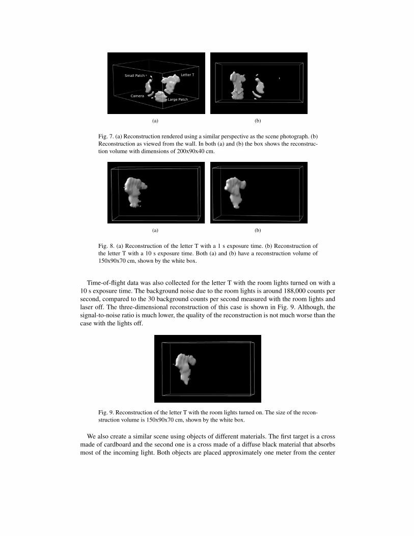
The first scene we reconstruct consists of the 38 x 41 cm letter T and the two white patches,placed so they span the entire reconstruction volume as shown in Fig. 3(a). The time-of-flightdata was collected with the lights off and an exposure time of 10 s. The resulting reconstructionis shown in Fig. 7.

All three objects in this scene are reconstructed at their correct positions (Fig. 7). An artifactis created by the specular reflection of the 1 inch filter on the camera. It appears at approx-imately the correct position and depth and does not interfere with the reconstruction of theremaining objects in the scene.

Using the letter T from the scene described above, data was collected again with the roomlights off using 1 s and 10 s exposure times to see how the signal to noise ratio effects recon-struction quality. As seen in Fig. 8, the 1 s exposure time (lower signal to noise ratio) resultedin a reconstruction with only slightly less defined edges compared to the 10 s exposure. In bothcases the general shape of the object is recovered.

Letter T

Large PatchCamera

Small Patch

(a) (b)

Fig. 7. (a) Reconstruction rendered using a similar perspective as the scene photograph. (b)Reconstruction as viewed from the wall. In both (a) and (b) the box shows the reconstruc-tion volume with dimensions of 200x90x40 cm.

(a) (b)

Fig. 8. (a) Reconstruction of the letter T with a 1 s exposure time. (b) Reconstruction ofthe letter T with a 10 s exposure time. Both (a) and (b) have a reconstruction volume of150x90x70 cm, shown by the white box.

Time-of-flight data was also collected for the letter T with the room lights turned on with a10 s exposure time. The background noise due to the room lights is around 188,000 counts persecond, compared to the 30 background counts per second measured with the room lights andlaser off. The three-dimensional reconstruction of this case is shown in Fig. 9. Although, thesignal-to-noise ratio is much lower, the quality of the reconstruction is not much worse than thecase with the lights off.

Fig. 9. Reconstruction of the letter T with the room lights turned on. The size of the recon-struction volume is 150x90x70 cm, shown by the white box.

We also create a similar scene using objects of different materials. The first target is a crossmade of cardboard and the second one is a cross made of a diffuse black material that absorbsmost of the incoming light. Both objects are placed approximately one meter from the center

of the projection area on the wall. Fig. 10 shows the 3D reconstructions of these targets. Al-though, both objects are detectable, the black cross is barely visible and the correct shape is notreconstructed.

10 cm

(a) (b)

10 cm

(c) (d)

Fig. 10. (a) The cardboard target. (b) The reconstruction of the cardboard target with a 10 sexposure. (c) The black target. (d) The reconstruction of the black target. For both (b) and(d), the reconstruction volume is 80x90x70 cm, shown by the white box.

5. Discussion

5.1. Resolution

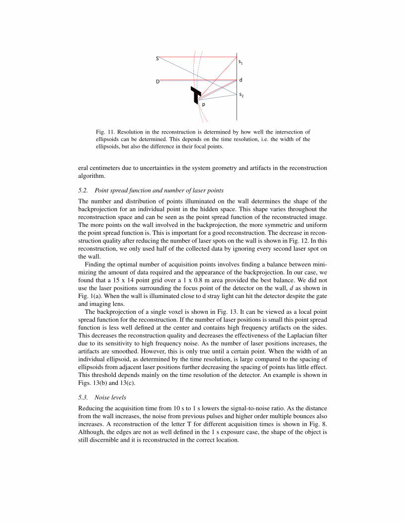
Our reconstruction method establishes object position by triangulation of distances calculatedusing time-of-flight information from different points on the laboratory wall. The accuracy ofthe distance calculation, and resulting position depend on the system’s time resolution and theseparation between the considered points on the wall (Fig. 11). One would expect that theangular resolution Θ behaves roughly as

Θ = 1.22cτ

a(1)

Where τ is the time resolution of the system and a is the largest distance between any twosample points on the wall in the entire pattern contributing to the reconstruction, and c is thespeed of light. This is analogous to the Rayleigh criterion for phase based optical and radarimaging. Our system has an angular resolution of (1.22·c·30ps)/1m = 0.0011 rad. Therefore,at a distance of 1 m from the wall we expect a resolution on the order of 1.1 cm. The actualresolution achieved as determined by the reconstructed feature size, is on the order of sev-

s1

p

s2

d

S

D

Fig. 11. Resolution in the reconstruction is determined by how well the intersection ofellipsoids can be determined. This depends on the time resolution, i.e. the width of theellipsoids, but also the difference in their focal points.

eral centimeters due to uncertainties in the system geometry and artifacts in the reconstructionalgorithm.

5.2. Point spread function and number of laser points

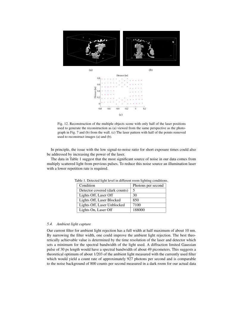
The number and distribution of points illuminated on the wall determines the shape of thebackprojection for an individual point in the hidden space. This shape varies throughout thereconstruction space and can be seen as the point spread function of the reconstructed image.The more points on the wall involved in the backprojection, the more symmetric and uniformthe point spread function is. This is important for a good reconstruction. The decrease in recon-struction quality after reducing the number of laser spots on the wall is shown in Fig. 12. In thisreconstruction, we only used half of the collected data by ignoring every second laser spot onthe wall.

Finding the optimal number of acquisition points involves finding a balance between mini-mizing the amount of data required and the appearance of the backprojection. In our case, wefound that a 15 x 14 point grid over a 1 x 0.8 m area provided the best balance. We did notuse the laser positions surrounding the focus point of the detector on the wall, d as shown inFig. 1(a). When the wall is illuminated close to d stray light can hit the detector despite the gateand imaging lens.

The backprojection of a single voxel is shown in Fig. 13. It can be viewed as a local pointspread function for the reconstruction. If the number of laser positions is small this point spreadfunction is less well defined at the center and contains high frequency artifacts on the sides.This decreases the reconstruction quality and decreases the effectiveness of the Laplacian filterdue to its sensitivity to high frequency noise. As the number of laser positions increases, theartifacts are smoothed. However, this is only true until a certain point. When the width of anindividual ellipsoid, as determined by the time resolution, is large compared to the spacing ofellipsoids from adjacent laser positions further decreasing the spacing of points has little effect.This threshold depends mainly on the time resolution of the detector. An example is shown inFigs. 13(b) and 13(c).

5.3. Noise levels

Reducing the acquisition time from 10 s to 1 s lowers the signal-to-noise ratio. As the distancefrom the wall increases, the noise from previous pulses and higher order multiple bounces alsoincreases. A reconstruction of the letter T for different acquisition times is shown in Fig. 8.Although, the edges are not as well defined in the 1 s exposure case, the shape of the object isstill discernible and it is reconstructed in the correct location.

(a) (b)

(c)

Fig. 12. Reconstruction of the multiple objects scene with only half of the laser positionsused to generate the reconstruction as (a) viewed from the same perspective as the photo-graph in Fig. 7 and (b) from the wall. (c) The laser pattern with half of the points removedused to reconstruct images (a) and (b).

In principle, the issue with the low signal-to-noise ratio for short exposure times could alsobe addressed by increasing the power of the laser.

The data in Table 1 suggest that the most significant source of noise in our data comes frommultiply scattered light from previous pulses. To reduce this noise source an illumination laserwith a lower repetition rate is required.

Table 1. Detected light level in different room lighting conditions.Condition Photons per secondDetector covered (dark counts) 5Lights Off, Laser Off 30Lights Off, Laser Blocked 850Lights Off, Laser Unblocked 7100Lights On, Laser Off 188000

5.4. Ambient light capture

Our current filter for ambient light rejection has a full width at half maximum of about 10 nm.By narrowing the filter width, one could improve the ambient light rejection. The best theo-retically achievable value is determined by the time resolution of the laser and detector whichsets a minimum for the spectral bandwidth of the light used. A diffraction limited Gaussianpulse of 30 ps length would have a spectral bandwidth of about 49 picometers. This suggests atheoretical optimum of about 1/203 of the ambient light measured with the currently used filterwhich would yield a count rate of approximately 927 photons per second and is comparableto the noise background of 800 counts per second measured in a dark room for our actual data

10cm

(a)

10cm

(b)

10cm

(c)

(d) (e) (f)

Fig. 13. The confidence map resulting from the backprojection of a point located 0.5 maway from the wall using different numbers of laser positions. (a) was created using the3x3 pattern shown in (d). (b) used the 6x6 pattern shown in (e), and (c) used the 11x11pattern shown in (f). In (d,e,f), the location of the target is shown by the o, the detectorlocation is represented by the x, and the laser origin is shown by the *

collection. This requires a laser with a range of tunability to tune it to a commercially availablenarrow band filter.

5.5. Capture speed

With a total capture time of several minutes, our current system is unsuitable for imaginingscenes with moving objects. To reduce the acquisition time required for a good reconstruction,it is possible to increase the laser intensity, introduce multi-point detection, or increase the col-lection area of the detector and the aperture of the lenses. One could be encouraged to keepthe laser intensity as low as possible for eye-safety, power dissipation, and cost reduction pur-poses. Finally, it would also be possible to replace the single SPAD with a 2D array of multipledetectors observing multiple patches on the wall simultaneously. By detecting photons at mul-tiple sources on the wall, multiple intersecting ellipsoids could be created in the backprojectionwith only one laser position, reducing the number of needed laser points and the total capturetime. This kind of detector has already been demonstrated [24] and recent developments onfully-integrated fast-gating circuits [25] will pave the way for producing a suitable monolithicarray of gated SPADs. With these methods, capture times can likely be reduced to fractions ofa second.

Unlike previous methods, our system is able to sample a grid of disconnected points on thewall. Previous systems were only able to image a connected area of pixels. Because of thissparse sampling of positions on the wall, the amount of data collected in this setup is relativelysmall.

5.6. Portability, cost reduction, and eye safety

In its current implementation, our system makes use of stand-alone components like the gated-mode SPAD module and the TCSPC module, used in combination with an high-performance

pulsed laser source and some ancillary instrumentation (scanning system, calibration camera,etc). The overall cost has been reduced compared to previous high time resolution, single pho-ton sensitive implementations [16], going from hundreds of thousands of dollars for a streakcamera to tens of thousands of dollars for the current setup. Beyond this, the real advantage ofour implementation is the potential integration of most of the components into a single, com-pact device such as a single integrated circuit. This has already happened for non-gated SPADarrays [24].

Both the gating and TCSPC electronics could be integrated into silicon and already exist inseparate chips. The detector is designed in a standard 0.35 µm CMOS technology, making itsuitable for integration with time-gating electronic circuits [25] (both in single and multi-pixelimplementations). High-performance 0.35 µm CMOS Time-to-Digital Converters (TDCs) havealready been proven to be an effective solution for TCSPC measurements, obtaining resolutionsof tens of picoseconds with extremely low power consumption [26]. This type of implemen-tation will take advantage of the cost reduction allowed by microelectronics miniaturization.By using it in combination with a pulsed laser diode, the overall system cost can be cut downto a few thousand dollars, or even less. Furthermore, the portability could benefit from theintegration process, giving rise to a compact, hand held, low-power device.

For field use, eye safety is a factor that needs to be taken under consideration. Our currentimplementation is not eye safe, however there are several things that could be done. Factorsaffecting the eye safety of a laser include the wavelength of light, scanning speed, and powerlevel of the beam. To avoid retina damage, a laser should have a wavelength between 1.4 and2 µm. Between these wavelengths, radiation does not penetrate more deeply than 100 µm intothe cornea [27] which has a higher damage threshold than the retina. To modify our systemto operate within the “eye-safe” range, we could use a mid-IR range laser with a InGaAs/InPSPAD rather than a silicon based one [28]. This would also lead to higher dark count rates ofthousands of counts per second and may not be advisable if dark count rates and not ambientlight are the limiting factor. On the other hand there are several frequency bands in this rangewhere sunlight does not effectively penetrate the atmosphere but attenuation levels are lowenough to not significantly attenuate a beam over hundreds of meters. Increased scanning speedcan lead to reduced laser dwell times and thus reduced average illumination intensity.

6. Conclusion

We demonstrate a novel photon counting non-line-of-sight imaging system based on a time-gated SPAD detector and demonstrate the ability to reconstruct images of part of our laboratoryvia the laboratory wall. We also study the sensitivity of the system towards noise and ambientlight.

Because of high loss in the propagation path it is essential to maximize the sensitivity, dy-namic range, and signal to noise ratio of non-line-of-sight imaging systems. For this reason, itis advantageous to use a sensitive high throughput photon counting detection system such asa gated SPAD. Photon counting is possible with a streak camera and iCCD cameras, but sinceonly a few photons are counted in each frame it takes a long time to build up sufficient photonnumbers for a reconstruction. The effective dynamic range of a gated SPAD is further increasedby blocking the first bounce light from the detector since this light is many orders of magnitudebrighter than the third bounce data required for reconstruction.

SPAD based non-line-of-sight imaging systems provide a promising option for compact, hightime resolution, and high sensitivity non-line-of-sight imaging systems.

Acknowledgments

We would like to acknowledge funding through the NASA NIAC Program (NNH14ZOA001N-14NIAC-A1), the Laboratory for Optical and Computational Instrumentation (LOCI), and theMorgridge Institute for Research. We would also like to thank Nick Bertone and PicoQuant forgenerously providing advice and equipment to support this research.