PH 393 Name Solution

Non-Linear Curve Fitting Exercises For each exercise below you are to provide the MATLAB m-files, which should contain a

clean copy from the command window showing the answers properly labeled as comments at

the end of the m-file. Clean copy means have the command window only show the answers

asked for. Please remove all excess spaces, blank lines, etc. Where asked paste into the

document as much as possible a full page plots with appropriate titles, axis labels, etc. Notice

I am using tables so add rows to put the plots in. If you need help see the professor. On my classes website http://physics.nmu.edu/~ddonovan/classes.html in the PH 393 section there is a link Data for Linear and Non-linear Curve Fitting Exercises. This will provide you with a zip file that contains data files to be used for these two sets of homework related to curve fitting. Download this file and extract the files to a folder in your MATLAB path so that you can load and use the data files. They are all two column data files in which the first column is the x data and the second is the f(x) or y data. You are to fill in this document and when it is completed with MATALB interspersed appropriately. (i.e. after problem 1 put the MATLAB work that belongs to problem 1, after problem 2, put the MATALAB work that belongs to problem 2 etc.) Email the completed file and a zip file containing all the MATLAB work. You can put this file into the Zip file if you wish. For each of the data files you are to complete the following steps:

a) Plot the raw data as a line on its own page. b) Use this plot to determine rough “starting guesses” for the parameters, you may draw in pencil on this plot to show how you arrived at the “starting guesses”. c) Find the parameters that provide “a reasonably good fit to the data”. If the fitted line does not look anything like the data, it is not “a reasonably good fit.” There are possible values of the parameters that provide very good fits. Do not quit with very bad fits. There will be little if any partial credit in such cases. If the program stops with a number of iterations exceeded message, you should start with the final parameters as your new starting guesses and see if you can get better convergence. You should try varying you final parameters some and see if you converge to a different set of parameters that might provide an even better fit. Do not settle for the first set of parameters you find.

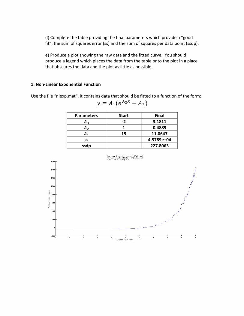
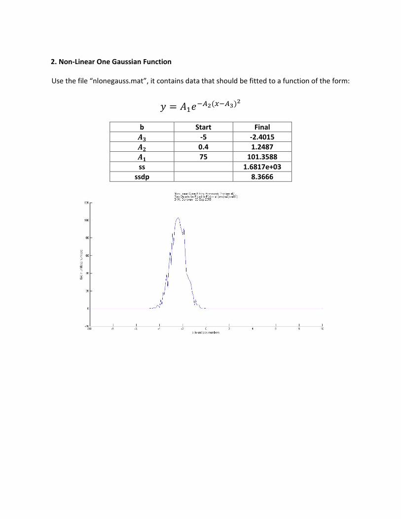
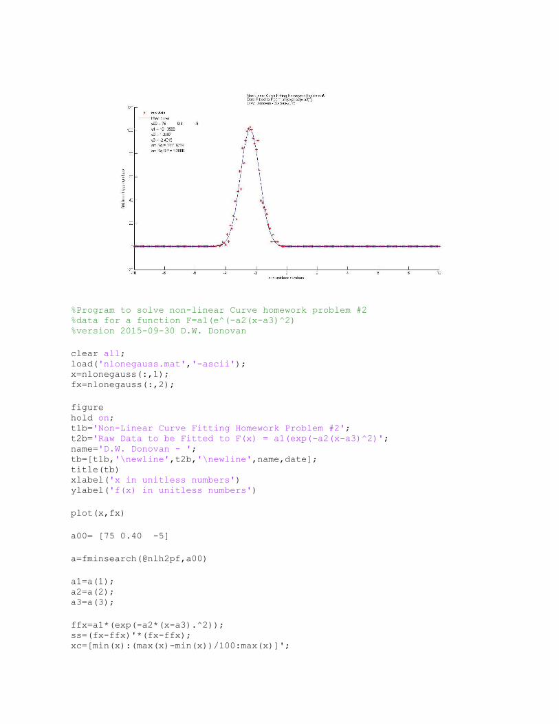
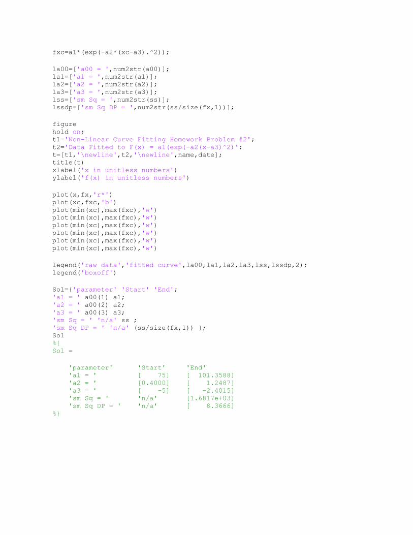
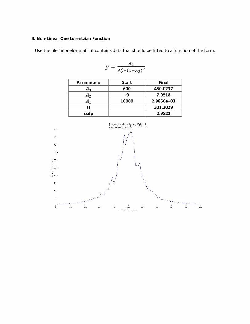
d) Complete the table providing the final parameters which provide a “good fit”, the sum of squares error (ss) and the sum of squares per data point (ssdp). e) Produce a plot showing the raw data and the fitted curve. You should produce a legend which places the data from the table onto the plot in a place that obscures the data and the plot as little as possible.

1. Non-Linear Exponential Function Use the file “nlexp.mat”, it contains data that should be fitted to a function of the form:

𝑦 = 𝐴1(𝑒𝐴2𝑥 − 𝐴3)

Parameters Start Final

𝑨𝟑 -2 3.1811

𝑨𝟐 1 0.4889

𝑨𝟏 15 11.0647

ss 4.5789e+04

ssdp 227.8063

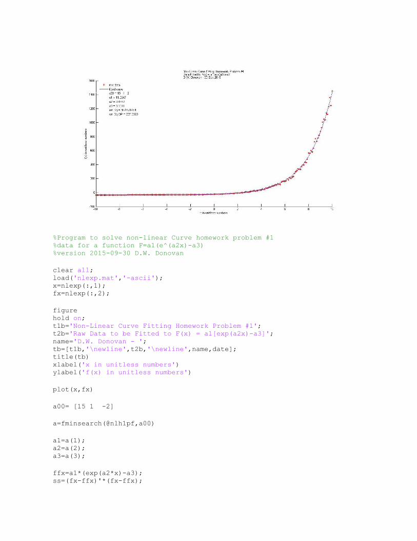
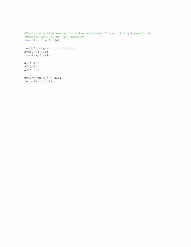
%Program to solve non-linear Curve homework problem #1 %data for a function F=a1(e^(a2x)-a3) %version 2015-09-30 D.W. Donovan

clear all; load('nlexp.mat','-ascii'); x=nlexp(:,1); fx=nlexp(:,2);

figure hold on; t1b='Non-Linear Curve Fitting Homework Problem #1'; t2b='Raw Data to be Fitted to F(x) = a1[exp(a2x)-a3]'; name='D.W. Donovan - '; tb=[t1b,'\newline',t2b,'\newline',name,date]; title(tb) xlabel('x in unitless numbers') ylabel('f(x) in unitless numbers')

plot(x,fx)

a00= [15 1 -2]

a=fminsearch(@nlh1pf,a00)

a1=a(1); a2=a(2); a3=a(3);

ffx=a1*(exp(a2*x)-a3); ss=(fx-ffx)'*(fx-ffx);

xc=[min(x):(max(x)-min(x))/100:max(x)]'; fxc=a1*(exp(a2*xc)-a3);

la00=['a00 = ',num2str(a00)]; la1=['a1 = ',num2str(a1)]; la2=['a2 = ',num2str(a2)]; la3=['a3 = ',num2str(a3)]; lss=['sm Sq = ',num2str(ss)]; lssdp=['sm Sq DP = ',num2str(ss/size(fx,1))];

figure hold on; t1='Non-Linear Curve Fitting Homework Problem #1'; t2='Data Fitted to F(x) = a1[exp(a2x)-a3]'; t=[t1,'\newline',t2,'\newline',name,date]; title(t) xlabel('x in unitless numbers') ylabel('f(x) in unitless numbers')

plot(x,fx,'r*') plot(xc,fxc,'b') plot(min(xc),max(fxc),'w') plot(min(xc),max(fxc),'w') plot(min(xc),max(fxc),'w') plot(min(xc),max(fxc),'w') plot(min(xc),max(fxc),'w') plot(min(xc),max(fxc),'w')

legend('raw data','fitted curve',la00,la1,la2,la3,lss,lssdp,2); legend('boxoff')

Sol={'parameter' 'Start' 'End'; 'a1 = ' a00(1) a1; 'a2 = ' a00(2) a2; 'a3 = ' a00(3) a3; 'sm Sq = ' 'n/a' ss; 'sm Sq DP = ' 'n/a' (ss/size(fx,1)) }; Sol %{ Sol =

'parameter' 'Start' 'End' 'a1 = ' [ 15] [ 11.0647] 'a2 = ' [ 1] [ 0.4889] 'a3 = ' [ -2] [ 3.1811] 'sm Sq = ' 'n/a' [4.5789e+04] 'sm Sq DP = ' 'n/a' [ 227.8063] %}

%Function m-file needed to solve nonlinear Curve fitting homework #1 %version 2007-10-08 D.W. Donovan function f = fun(a)

load('nlexp.mat','-ascii'); x=nlexp(:,1); fx=nlexp(:,2);

a1=a(1); a2=a(2); a3=a(3);

g=a1*(exp(a2*x)-a3); f=(g-fx)'*(g-fx);

2. Non-Linear One Gaussian Function Use the file “nlonegauss.mat”, it contains data that should be fitted to a function of the form:

𝑦 = 𝐴1𝑒−𝐴2(𝑥−𝐴3)

2

b Start Final

𝑨𝟑 -5 -2.4015

𝑨𝟐 0.4 1.2487

𝑨𝟏 75 101.3588

ss 1.6817e+03

ssdp 8.3666

%Program to solve non-linear Curve homework problem #2 %data for a function F=a1(e^(-a2(x-a3)^2) %version 2015-09-30 D.W. Donovan

clear all; load('nlonegauss.mat','-ascii'); x=nlonegauss(:,1); fx=nlonegauss(:,2);

figure hold on; t1b='Non-Linear Curve Fitting Homework Problem #2'; t2b='Raw Data to be Fitted to F(x) = a1(exp(-a2(x-a3)^2)'; name='D.W. Donovan - '; tb=[t1b,'\newline',t2b,'\newline',name,date]; title(tb) xlabel('x in unitless numbers') ylabel('f(x) in unitless numbers')

plot(x,fx)

a00= [75 0.40 -5]

a=fminsearch(@nlh2pf,a00)

a1=a(1); a2=a(2); a3=a(3);

ffx=a1*(exp(-a2*(x-a3).^2)); ss=(fx-ffx)'*(fx-ffx); xc=[min(x):(max(x)-min(x))/100:max(x)]';

fxc=a1*(exp(-a2*(xc-a3).^2));

la00=['a00 = ',num2str(a00)]; la1=['a1 = ',num2str(a1)]; la2=['a2 = ',num2str(a2)]; la3=['a3 = ',num2str(a3)]; lss=['sm Sq = ',num2str(ss)]; lssdp=['sm Sq DP = ',num2str(ss/size(fx,1))];

figure hold on; t1='Non-Linear Curve Fitting Homework Problem #2'; t2='Data Fitted to F(x) = a1(exp(-a2(x-a3)^2)'; t=[t1,'\newline',t2,'\newline',name,date]; title(t) xlabel('x in unitless numbers') ylabel('f(x) in unitless numbers')

plot(x,fx,'r*') plot(xc,fxc,'b') plot(min(xc),max(fxc),'w') plot(min(xc),max(fxc),'w') plot(min(xc),max(fxc),'w') plot(min(xc),max(fxc),'w') plot(min(xc),max(fxc),'w') plot(min(xc),max(fxc),'w')

legend('raw data','fitted curve',la00,la1,la2,la3,lss,lssdp,2); legend('boxoff')

Sol={'parameter' 'Start' 'End'; 'a1 = ' a00(1) a1; 'a2 = ' a00(2) a2; 'a3 = ' a00(3) a3; 'sm Sq = ' 'n/a' ss ; 'sm Sq DP = ' 'n/a' (ss/size(fx,1)) }; Sol %{ Sol =

'parameter' 'Start' 'End' 'a1 = ' [ 75] [ 101.3588] 'a2 = ' [0.4000] [ 1.2487] 'a3 = ' [ -5] [ -2.4015] 'sm Sq = ' 'n/a' [1.6817e+03] 'sm Sq DP = ' 'n/a' [ 8.3666] %}

%Function m-file needed to solve nonlinear Curve fitting homework #2 %version 2007-10-08 D.W. Donovan function f = fun(a)

load('nlonegauss.mat','-ascii'); x=nlonegauss(:,1); fx=nlonegauss(:,2);

a1=a(1); a2=a(2); a3=a(3);

g=a1*(exp(-a2*(x-a3).^2)); f=(g-fx)'*(g-fx);

3. Non-Linear One Lorentzian Function

Use the file “nlonelor.mat”, it contains data that should be fitted to a function of the form:

𝑦 =𝐴1

𝐴22+(𝑥−𝐴3)

2

Parameters Start Final

𝑨𝟑 600 450.0237

𝑨𝟐 -9 7.9518

𝑨𝟏 10000 2.9856e+03

ss 301.2029

ssdp 2.9822

%Program to solve non-linear Curve homework problem #3 %data for a function F=a1/(a2^2+(x-a3)^2) %version 2015-09-30 D.W. Donovan

clear all; load('nlonelor.mat','-ascii'); x=nlonelor(:,1); fx=nlonelor(:,2);

figure hold on; t1b='Non-Linear Curve Fitting Homework Problem #3'; t2b='Raw Data to be Fitted to F(x) = a1/(a2^2+(x-a3)^2)'; name='D.W. Donovan - '; tb=[t1b,'\newline',t2b,'\newline',name,date]; title(tb) xlabel('x in unitless numbers') ylabel('f(x) in unitless numbers')

plot(x,fx)

a00= [10000 -9 600];

a=fminsearch(@nlh3pf,a00);

a1=a(1); a2=a(2); a3=a(3);

ffx=a1./(a2.^2+(x-a3).^2); ss=(fx-ffx)'*(fx-ffx); xc=[min(x):(max(x)-min(x))/100:max(x)]';

fxc=a1./(a2.^2+(xc-a3).^2);

la00=['a00 = ',num2str(a00)]; la1=['a1 = ',num2str(a1)]; la2=['a2 = ',num2str(a2)]; la3=['a3 = ',num2str(a3)]; lss=['sm Sq = ',num2str(ss)]; lssdp=['sm Sq DP = ',num2str(ss/size(fx,1))];

figure hold on; t1='Non-Linear Curve Fitting Homework Problem #3'; t2='Data Fitted to F(x) = a1/(a2^2+(x-a3)^2)'; t=[t1,'\newline',t2,'\newline',name,date]; title(t) xlabel('x in unitless numbers') ylabel('f(x) in unitless numbers')

plot(x,fx,'r*') plot(xc,fxc,'b') plot(min(xc),max(fxc),'w') plot(min(xc),max(fxc),'w') plot(min(xc),max(fxc),'w') plot(min(xc),max(fxc),'w') plot(min(xc),max(fxc),'w') plot(min(xc),max(fxc),'w')

legend('raw data','fitted curve',la00,la1,la2,la3,lss,lssdp,2); legend('boxoff')

Sol={'parameter' 'Start' 'End'; 'a1 = ' a00(1) a1; 'a2 = ' a00(2) a2; 'a3 = ' a00(3) a3; 'sm Sq = ' 'n/a' ss ; 'sm Sq DP = ' 'n/a' (ss/size(fx,1))}; Sol %{ Sol =

'parameter' 'Start' 'End' 'a1 = ' [10000] [2.9856e+03] 'a2 = ' [ -9] [ 7.9518] 'a3 = ' [ 600] [ 450.0237] 'sm Sq = ' 'n/a' [ 301.2029] 'sm Sq DP = ' 'n/a' [ 2.9822] %}

%Function m-file needed to solve nonlinear Curve fitting homework #3 %version 2007-10-08 D.W. Donovan function f = fun(a)

load('nlonelor.mat','-ascii'); x=nlonelor(:,1); fx=nlonelor(:,2);

a1=a(1); a2=a(2); a3=a(3);

g=a1./(a2.^2+(x-a3).^2); f=(g-fx)'*(g-fx);

4. Non-Linear Two Gaussian Functions Use the file “nltwogauss.mat”, it contains data that should be fitted to a function of the form:

𝑦 = 𝐴1𝑒−𝐴2(𝑥−𝐴3)

2+ 𝐴4𝑒

−𝐴5(𝑥−𝐴6)2

Parameters Start Final

𝑨𝟔 65 54.9846

𝑨𝟓 0.47 0.6144

𝑨𝟒 5 12.2136

𝑨𝟑 50 51.9718

𝑨𝟐 0.25 0.2674

𝑨𝟏 5 9.9135

ss 16.5612

ssdp 0.0207

%Program to solve non-linear Curve homework problem #4 %data for a function F=a1(e^(-a2(x-a3)^2) %version 2015-09-30 D.W. Donovan

clear all; load('nltwogauss.mat','-ascii'); x=nltwogauss(:,1); fx=nltwogauss(:,2);

figure hold on; t1b='Non-Linear Curve Fitting Homework Problem #4'; t2b='Raw Data to be Fitted to F(x) = a1(exp(-a2(x-a3)^2) + a4(exp(-a5(x-

a6)^2)'; name='D.W. Donovan - '; tb=[t1b,'\newline',t2b,'\newline',name,date]; title(tb) xlabel('x in unitless numbers') ylabel('f(x) in unitless numbers')

plot(x,fx)

a00=[5 .25 50 5 0.47 65];

a=fminsearch(@nlh4pf,a00);

a1=a(1); a2=a(2); a3=a(3); a4=a(4); a5=a(5); a6=a(6);

ffx1=a1*(exp(-a2*(x-a3).^2)); ffx2=a4*(exp(-a5*(x-a6).^2)); ffx=ffx1+ffx2;

ss=(fx-ffx)'*(fx-ffx); xc=[min(x):(max(x)-min(x))/100:max(x)]'; fxc1=a1*(exp(-a2*(xc-a3).^2)); fxc2=a4*(exp(-a5*(xc-a6).^2)); fxc=fxc1+fxc2;

la00=['a00 = ',num2str(a00)]; la1=['a1 = ',num2str(a1)]; la2=['a2 = ',num2str(a2)]; la3=['a3 = ',num2str(a3)]; la4=['a4 = ',num2str(a4)]; la5=['a5 = ',num2str(a5)]; la6=['a6 = ',num2str(a6)]; lss=['sm Sq = ',num2str(ss)]; lssdp=['sm Sq DP = ',num2str(ss/size(fx,1))];

figure hold on; t1='Non-Linear Curve Fitting Homework Problem #4'; t2='Data Fitted to F(x) = a1(exp(-a2(x-a3)^2)+ a4(exp(-a5(x-a6)^2)'; t=[t1,'\newline',t2,'\newline',name,date]; title(t) xlabel('x in unitless numbers') ylabel('f(x) in unitless numbers')

plot(x,fx,'r*') plot(xc,fxc,'b') plot(min(xc),max(fxc),'w') plot(min(xc),max(fxc),'w') plot(min(xc),max(fxc),'w') plot(min(xc),max(fxc),'w') plot(min(xc),max(fxc),'w') plot(min(xc),max(fxc),'w') plot(min(xc),max(fxc),'w') plot(min(xc),max(fxc),'w') plot(min(xc),max(fxc),'w')

legend('raw data','fitted curve',la00,la1,la2,la3,la4,la5,la6,lss,lssdp,2); legend('boxoff')

Sol={'parameter' 'Start' 'End'; 'a1 = ' a00(1) a1; 'a2 = ' a00(2) a2; 'a3 = ' a00(3) a3; 'a4 = ' a00(4) a4; 'a5 = ' a00(5) a5; 'a6 = ' a00(6) a6; 'sm Sq = ' 'n/a' ss ; 'sm Sq DP = ' 'n/a' (ss/size(fx,1)) }; Sol

%{ Sol =

'parameter' 'Start' 'End' 'a1 = ' [ 5] [ 9.9135] 'a2 = ' [0.2500] [ 0.2674] 'a3 = ' [ 50] [51.9718] 'a4 = ' [ 5] [12.2136] 'a5 = ' [0.4700] [ 0.6144] 'a6 = ' [ 65] [54.9846] 'sm Sq = ' 'n/a' [16.5612] 'sm Sq DP = ' 'n/a' [ 0.0207] %}

%Function m-file needed to solve nonlinear Curve fitting homework #4 %version 2007-10-09 D.W. Donovan function f = fun(a)

load('nltwogauss.mat','-ascii'); x=nltwogauss(:,1); fx=nltwogauss(:,2);

a1=a(1); a2=a(2); a3=a(3); a4=a(4); a5=a(5); a6=a(6);

g1=a1*(exp(-a2*(x-a3).^2)); g2=a4*(exp(-a5*(x-a6).^2)); g=g1+g2;

f=(g-fx)'*(g-fx);

5. Non-Linear Two Lorentzian Functions Use the file “nltwolor.mat”, it contains data that should be fitted to a function of the form:

𝑦 =𝐴1

𝐴22 + (𝑥 − 𝐴3)

2+

𝐴4

𝐴52 + (𝑥 − 𝐴6)

2

Parameters Start Final

𝑨𝟔 1350 1.2999e+03

𝑨𝟓 3.5 3.8828

𝑨𝟒 4000 3.9799e+03

𝑨𝟑 1200 1.2502e+03

𝑨𝟐 8 7.7802

𝑨𝟏 3000 2.9453e+03

ss 1.2754e+04

ssdp 25.4561

%Program to solve non-linear Curve homework problem #5 %data for a function F=a1/(a2^2+(x-a3)^2)+a4/(a5^2+(x-a6)^2 %version 2015-09-30 D.W. Donovan

clear all; load('nltwolor.mat','-ascii'); x=nltwolor(:,1); fx=nltwolor(:,2);

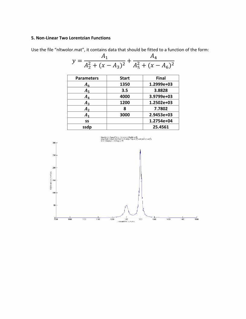
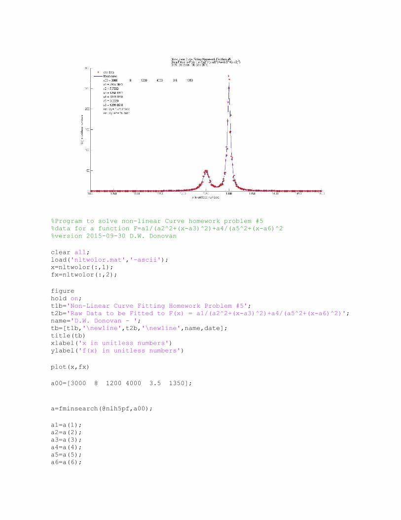
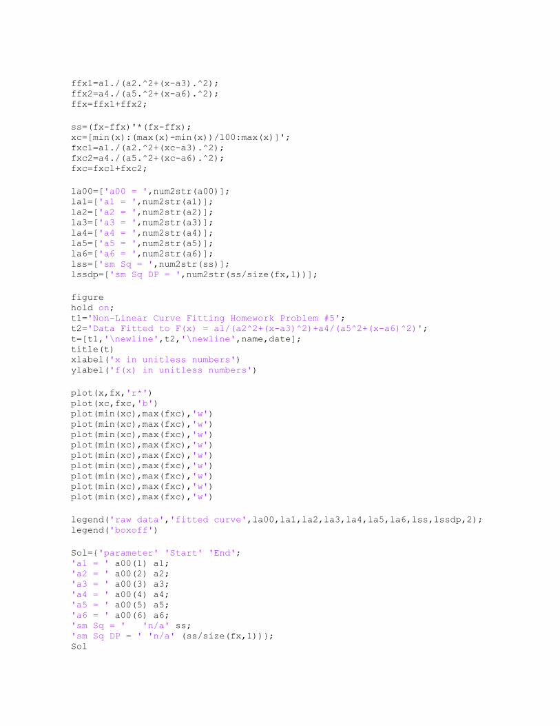
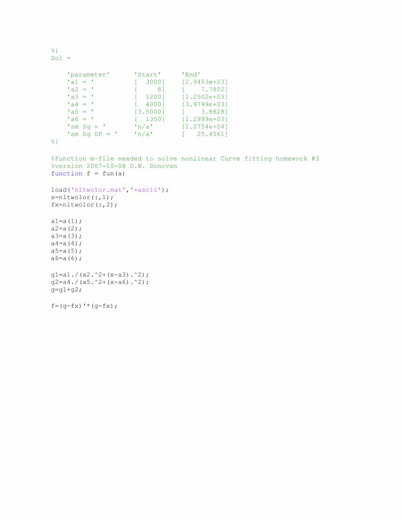
figure hold on; t1b='Non-Linear Curve Fitting Homework Problem #5'; t2b='Raw Data to be Fitted to F(x) = a1/(a2^2+(x-a3)^2)+a4/(a5^2+(x-a6)^2)'; name='D.W. Donovan - '; tb=[t1b,'\newline',t2b,'\newline',name,date]; title(tb) xlabel('x in unitless numbers') ylabel('f(x) in unitless numbers')

plot(x,fx)

a00=[3000 8 1200 4000 3.5 1350];

a=fminsearch(@nlh5pf,a00);

a1=a(1); a2=a(2); a3=a(3); a4=a(4); a5=a(5); a6=a(6);

ffx1=a1./(a2.^2+(x-a3).^2); ffx2=a4./(a5.^2+(x-a6).^2); ffx=ffx1+ffx2;

ss=(fx-ffx)'*(fx-ffx); xc=[min(x):(max(x)-min(x))/100:max(x)]'; fxc1=a1./(a2.^2+(xc-a3).^2); fxc2=a4./(a5.^2+(xc-a6).^2); fxc=fxc1+fxc2;

la00=['a00 = ',num2str(a00)]; la1=['a1 = ',num2str(a1)]; la2=['a2 = ',num2str(a2)]; la3=['a3 = ',num2str(a3)]; la4=['a4 = ',num2str(a4)]; la5=['a5 = ',num2str(a5)]; la6=['a6 = ',num2str(a6)]; lss=['sm Sq = ',num2str(ss)]; lssdp=['sm Sq DP = ',num2str(ss/size(fx,1))];

figure hold on; t1='Non-Linear Curve Fitting Homework Problem #5'; t2='Data Fitted to F(x) = a1/(a2^2+(x-a3)^2)+a4/(a5^2+(x-a6)^2)'; t=[t1,'\newline',t2,'\newline',name,date]; title(t) xlabel('x in unitless numbers') ylabel('f(x) in unitless numbers')

plot(x,fx,'r*') plot(xc,fxc,'b') plot(min(xc),max(fxc),'w') plot(min(xc),max(fxc),'w') plot(min(xc),max(fxc),'w') plot(min(xc),max(fxc),'w') plot(min(xc),max(fxc),'w') plot(min(xc),max(fxc),'w') plot(min(xc),max(fxc),'w') plot(min(xc),max(fxc),'w') plot(min(xc),max(fxc),'w')

legend('raw data','fitted curve',la00,la1,la2,la3,la4,la5,la6,lss,lssdp,2); legend('boxoff')

Sol={'parameter' 'Start' 'End'; 'a1 = ' a00(1) a1; 'a2 = ' a00(2) a2; 'a3 = ' a00(3) a3; 'a4 = ' a00(4) a4; 'a5 = ' a00(5) a5; 'a6 = ' a00(6) a6; 'sm Sq = ' 'n/a' ss; 'sm Sq DP = ' 'n/a' (ss/size(fx,1))}; Sol

%{ Sol =

'parameter' 'Start' 'End' 'a1 = ' [ 3000] [2.9453e+03] 'a2 = ' [ 8] [ 7.7802] 'a3 = ' [ 1200] [1.2502e+03] 'a4 = ' [ 4000] [3.9799e+03] 'a5 = ' [3.5000] [ 3.8828] 'a6 = ' [ 1350] [1.2999e+03] 'sm Sq = ' 'n/a' [1.2754e+04] 'sm Sq DP = ' 'n/a' [ 25.4561] %}

%Function m-file needed to solve nonlinear Curve fitting homework #3 %version 2007-10-08 D.W. Donovan function f = fun(a)

load('nltwolor.mat','-ascii'); x=nltwolor(:,1); fx=nltwolor(:,2);

a1=a(1); a2=a(2); a3=a(3); a4=a(4); a5=a(5); a6=a(6);

g1=a1./(a2.^2+(x-a3).^2); g2=a4./(a5.^2+(x-a6).^2); g=g1+g2;

f=(g-fx)'*(g-fx);