Brazilian Journal of Animal Science e-ISSN 1806-9290 www.rbz.org.br R. Bras. Zootec., 49:e20190201, 2020 https://doi.org/10.37496/rbz4920190201 Non-ruminants Full-length research article Non-linear mixed models in the study of growth of naturalized chickens ABSTRACT - This study was conducted to examine the inclusion of random effects in non-linear models, identify the most suitable models, and describe the growth of naturalized chickens. Live-weight records of 166 birds of the Graúna Dourada, Nordestina, and Teresina ecotypes were estimated. The asymptotic weight (A), integration constant, related to animal initial weight (B), and the maturing rate (k) parameters of the non-linear Gompertz, Logistic, and von Bertalanffy models were estimated and adjusted using the Gauss-Newton method. Residual variance decreased by more than 50% when random effects were added to the model. The best fits in the estimate of the growth curve of females were obtained by associating the random effects with the three parameters of the Gompertz and Logistic models. The association of random effects with two parameters (asymptotic weight and maturing rate) and with the three parameters of the Logistic model provided the best fits for the males. The Teresina ecotype has the highest adult weight in both sexes, despite its slower growth. The opposite is true for the Graúna Dourada ecotype, formed by lighter and earlier- growing animals. The inclusion of random effects in models provides greater accuracy in the estimate of the growth curve. Keywords: Gompertz, modelling, phenotypic variation, rooster Introduction Chickens were introduced in Brazil at the time of its discovery and colonization. The chicken groups that were not subjected to any breeding method and that adapted to the rearing conditions and to the environment in which they were managed were named “naturalized” chickens. Several ecotypes of the species were extinguished after the introduction of genetically improved breeds and lines from other countries. Some groups are being subjected to genetic conservation in teaching and research institutions. However, little information exists on the production rates and growth of those animals. Non-linear models allow for a comparison of the growth curve of different genetic groups, making it possible to evaluate differences in animal growth caused by sex, management, and rearing environment. They also provide essential information to guide the sustainable preservation of animals at risk of extinction, such as the estimate of nutritional requirements and growth (Hruby et al., 1994; Selvaggi et al., 2015). Vicente Ibiapina Neto 1 , Firmino José Vieira Barbosa 2 , José Elivalto Guimarães Campelo 3 , José Lindenberg Rocha Sarmento 3* 1 Universidade Federal Piauí, Programa de Pós-Graduação em Ciência Animal, Teresina, PI, Brasil. 2 Universidade Estadual do Piauí, Centro de Ciências Agrárias, Teresina, PI, Brasil. 3 Universidade Federal do Piauí, Departamento de Zootecnia, Teresina, PI, Brasil. *Corresponding author: [email protected]Received: September 26, 2019 Accepted: March 12, 2020 How to cite: Ibiapina Neto, V.; Barbosa, F. J. V.; Campelo, J. E. G. and Sarmento, J. L. R. 2020. Non-linear mixed models in the study of growth of naturalized chickens. Revista Brasileira de Zootecnia 49:e20190201. https://doi.org/10.37496/rbz4920190201 Copyright: This is an open access article distributed under the terms of the Creative Commons Attribution License (http://creativecommons.org/licenses/by/4.0/), which permits unrestricted use, distribution, and reproduction in any medium, provided the original work is properly cited.
Transcript
Brazilian Journal of Animal Sciencee-ISSN 1806-9290www.rbz.org.br
R. Bras. Zootec., 49:e20190201, 2020https://doi.org/10.37496/rbz4920190201
Non-ruminantsFull-length research article
Non-linear mixed models in the study of growth of naturalized chickens
ABSTRACT - This study was conducted to examine the inclusion of random effects in non-linear models, identify the most suitable models, and describe the growth of naturalized chickens. Live-weight records of 166 birds of the Graúna Dourada, Nordestina, and Teresina ecotypes were estimated. The asymptotic weight (A), integration constant, related to animal initial weight (B), and the maturing rate (k) parameters of the non-linear Gompertz, Logistic, and von Bertalanffy models were estimated and adjusted using the Gauss-Newton method. Residual variance decreased by more than 50% when random effects were added to the model. The best fits in the estimate of the growth curve of females were obtained by associating the random effects with the three parameters of the Gompertz and Logistic models. The association of random effects with two parameters (asymptotic weight and maturing rate) and with the three parameters of the Logistic model provided the best fits for the males. The Teresina ecotype has the highest adult weight in both sexes, despite its slower growth. The opposite is true for the Graúna Dourada ecotype, formed by lighter and earlier-growing animals. The inclusion of random effects in models provides greater accuracy in the estimate of the growth curve.
Chickens were introduced in Brazil at the time of its discovery and colonization. The chicken groups that were not subjected to any breeding method and that adapted to the rearing conditions and to the environment in which they were managed were named “naturalized” chickens.
Several ecotypes of the species were extinguished after the introduction of genetically improved breeds and lines from other countries. Some groups are being subjected to genetic conservation in teaching and research institutions. However, little information exists on the production rates and growth of those animals.
Non-linear models allow for a comparison of the growth curve of different genetic groups, making it possible to evaluate differences in animal growth caused by sex, management, and rearing environment. They also provide essential information to guide the sustainable preservation of animals at risk of extinction, such as the estimate of nutritional requirements and growth (Hruby et al., 1994; Selvaggi et al., 2015).
Vicente Ibiapina Neto1 , Firmino José Vieira Barbosa2 , José Elivalto Guimarães Campelo3 , José Lindenberg Rocha Sarmento3*
1 Universidade Federal Piauí, Programa de Pós-Graduação em Ciência Animal, Teresina, PI, Brasil.
2 Universidade Estadual do Piauí, Centro de Ciências Agrárias, Teresina, PI, Brasil. 3 Universidade Federal do Piauí, Departamento de Zootecnia, Teresina, PI, Brasil.
*Corresponding author: [email protected]: September 26, 2019Accepted: March 12, 2020How to cite: Ibiapina Neto, V.; Barbosa, F. J. V.; Campelo, J. E. G. and Sarmento, J. L. R. 2020. Non-linear mixed models in the study of growth of naturalized chickens. Revista Brasileira de Zootecnia 49:e20190201. https://doi.org/10.37496/rbz4920190201
Copyright: This is an open access articledistributed under the terms of theCreative Commons Attribution License(http://creativecommons.org/licenses/by/4.0/),which permits unrestricted use, distribution,and reproduction in any medium, provided theoriginal work is properly cited.
Non-linear mixed models in the study of growth of naturalized chickensIbiapina Neto et al.
2
In studies on growth curves, some basic principles should be taken into account for the efficient use of non-linear models. One of such principles is that the data must present homogeneity of variance and residuals must not be correlated.
Nevertheless, longitudinal data derived from growth studies may exhibit different variances throughout the animal’s life. Moreover, repeated measures from the same individual provide correlated residuals, compromising the efficient use of these models, which are assumed to be fixed (Guedes et al., 2004; Mazucheli et al., 2011).
An alternative to address this problem is the incorporation of random effects associated with the individuals into the model, thus characterizing it as a non-linear mixed model. The use of this type of model makes it possible to adjust flexible covariance structures capable of handling imbalanced data (Lindstrom and Bates, 1990).
Non-linear mixed models have been applied in studies on the growth pattern of quail (Karaman et al., 2013) and birds (Sofaer et al., 2013), to estimate metabolizable energy utilization by chickens (Romero et al., 2009), estimate the nutritional requirements of laying hens (Strathe et al., 2011), among others. However, there are no reports of the use of methodologies to describe the growth pattern of naturalized chickens.
Therefore, this study proposes to evaluate the inclusion of random effects in non-linear mixed models to describe the growth curve of naturalized chickens.
Material and Methods
The study was conducted after approval by the institutional Animal Use Committee (case no. 404/17). A database was used with live-weight records (collected fortnightly) of 166 birds of the Graúna Dourada (53 females and 38 males), Nordestina (19 females and 17 males), and Teresina (16 females and 23 males; Figure 1) ecotypes, located in Teresina, PI - Brazil (5°03'57.2" S, 42°42'09.2" W), with a minimum number of five weights per bird.
Figure 1 - Residuals standardized for the models that best described the growth of naturalized chicken ecotypes.
FemalesGraúna Dourada
MalesGraúna Dourada
(y1) (y2) (y3) (y4)
Stan
dard
ized
resi
dual
s
2
0
–2
0 50 100 150 200Age (days)
0 50 100 150 200Age (days)
0 50 100 150 200Age (days)
0 50 100 150 200Age (days)
Stan
dard
ized
resi
dual
s
2
0
–2
Stan
dard
ized
resi
dual
s
2
0
–2
3210
–1–2–3St
anda
rdiz
ed re
sidu
als
Stan
dard
ized
resi
dual
s
0 50 100 150 200Age (days)
0 50 100 150 200Age (days)
0 50 100 150 200Age (days)
0 50 100 150 200Age (days)
2
1
0
–1
–2
2
1
0
–1
–2
210
–1–2
2
1
0
–1
–2–3St
anda
rdiz
ed re
sidu
als
Stan
dard
ized
resi
dual
s
Stan
dard
ized
resi
dual
s
Nordestina
Teresina
Nordestina
Teresina
0 50 100 150Age (days)
0 50 100 150Age (days)
0 50 100 150 200Age (days)
0 50 100 150 200Age (days)
210
–1–2–3St
anda
rdiz
ed re
sidu
als 3
210
–1–2–3St
anda
rdiz
ed re
sidu
als 3
210
–1–2–3St
anda
rdiz
ed re
sidu
als
2
1
0
–1
–2
Stan
dard
ized
resi
dual
s 3
R. Bras. Zootec., 49:e20190201, 2020
Non-linear mixed models in the study of growth of naturalized chickensIbiapina Neto et al.
3
The chicks were weighed at birth and then housed in proper metal cages equipped with a feeder, a drinker, and a heating source for the first weeks of life. The animals were divided into four age ranges, in which the supplied feed would meet their respective requirements. The diet provided in the pre-starter phase, from the 1st to the 30th day of life, was composed of 630 g/kg corn, 320 g/kg soybean meal, and 50 g/kg vitamin-mineral mix (Núcleo Fit Aves Pré-Inicial®, Poli Nutri, Brazil). In the starter phase, from the 30th to the 60th day of life, the feed composition was 660 g/kg corn, 290 g/kg soybean meal, and 50 g/kg vitamin-mineral mix (Núcleo Fit Aves Inicial®, Poli Nutri, Brazil). This was followed by the grower phase, from the 60th day of life until the appearance of the first signs of reproduction, which occurred at around 180 days of life (feed composition: 700 g/kg corn, 250 g/kg soybean meal, and 50 g/kg vitamin-mineral mix [Núcleo Fit Aves Engorda®, Poli Nutri, Brazil]). Lastly, in the finisher phase, which started on the 180th day of life, the birds received a diet composed of 630 g/kg corn, 245 g/kg soybean meal, 85 g/kg calcitic limestone, and 40 g/kg vitamin-mineral mix (Núcleo Poli Macro Ovo 4%®, Poli Nutri, Brazil). The pre-starter, starter, grower, and finisher diets had approximate protein (g/kg) and energy (MJ/kg) contents of 195 and 11.9, 185 and 12.1, 170 and 12.3, and 160 and 11.3, respectively.
The linear models can be described as follows:
yij = f (βi, xij) + εij, εij~N(0, σe2),
in which yij is the j-th observation of individual I, f is a non-linear function of a parameter vector βi and a vector xij of prediction of yij, and εij is a normal-distribution error. The parameter vector can vary between the individuals and is incorporated into the model as shown below:
βi = Aiβ + Bibi, bi~N(0, σ2D),
in which β is a vector of parameters of fixed effects associated with the population; bi is a vector of random effects associated with individuals i; Ai and Bi are incidence matrices of the fixed and random effects, respectively; and σ2D is a matrix of covariances between the random effects (Lindstrom and Bates, 1990).
To adjust the growth curve, the A, B, and k parameters of the Gompertz (Laird, 1965), Logistic (Nelder, 1961), and von Bertalanffy (Bertalanffy, 1957) models were estimated using the Gauss-Newton method, described by Hartley (1961) for non-linear models.
In the non-linear mixed models, the random effects are associated with the parameters. For the Gompertz, Logistic, and von Bertalanffy models, it is possible to compare seven possibilities of addition of random effects. The present study tested a model without random effects, named “non-linear model of fixed effects”; three models with addition of only one random effect; three models with addition of two random effects; and one model with addition of random effect on the three parameters (Table 1).
The models were compared by using the following criteria for the choice of the model that best fit the growth curve: the mean squared error (MSE), calculated by dividing the sum of residual squares by the number of observations; the average absolute deviation of residuals (AAD), described by Sarmento et al. (2006), calculated as the sum of the module or absolute values of the residuals divided by the number of observations; and the coefficient of determination (R²), obtained from the calculation of the square of the correlation between observed and estimated weights.
Akaike’s Information Criterion (AIC) (Akaike, 1974) and the Bayesian Information Criterion (BIC) (Schwarz, 1978) were also used for the choice of the best-fitting model. The values were obtained as follows: AIC = –2logL(θ̂) + 2 (p) and BIC = –2logL(θ̂) + ln(N)p, in which p represents the total number of parameters estimated by the model, N is the total number of observations, and logL(θ̂) is the logarithm of restricted likelihood.
R. Bras. Zootec., 49:e20190201, 2020
Non-linear mixed models in the study of growth of naturalized chickensIbiapina Neto et al.
4
Age (ti) and weight (yi) at the inflection point were calculated using the equations ti = (lnB)/k and yi = A/2 for the Logistic model; ti = (logB)/k and yi = A/e for the Gompertz model; and ti = loge(3b)/k and yi = 8A/27 for the von Bertalanffy model.
R software was used to estimate the parameters and to adjust the non-linear models, applying the nls (Nonlinear Least Squares) function of the Stats package and the nlme (Nonlinear Mixed-Effects Models) package. The maximum likelihood method was employed to estimate the mixed-model parameters, using the algorithm created by Lindstrom and Bates (1990) for integer approximation.
The same software was used to compare and group the similar models via Tocher’s optimization method. For this, the values from the evaluation of fitting criteria of the adjusted models were subjected to the Tocher function in the BioTools package of R software (R Core Team, 2017). Pearson’s correlations between the parameters were obtained using the Stats package of R software.
Results
The Gompertz model with random effects associated with the A and k parameters estimated similar asymptotic weights between the two sexes. However, in the other tested models, a significant difference was observed between males and females for this parameter (Table 2).
Table 1 - Models without and with random effect proposed to explain the growth pattern of naturalized chickensModel Random effect Formula
von Bertalanffy Absent y = A(1 – Bexp(–kt))3
A y = (A + u1)(1 – Bexp(–kt))3
B y = A(1 – (B + u2)exp(–kt))3
k y = A(1 – Bexp(–(k + u3)t))3
A and B y = (A + u1)(1 – (B + u2)exp(–kt))3
A and k y = (A + u1)(1 – Bexp(–(k + u3)t))3
B and k y = A(1 – (B + u2)exp(–(k + u3)t))3
A, B, and k y = (A + u1)(1 – (B + u2)exp(–(k + u3)t))3
Gompertz Absent y = Aexp(–Bexp(–kt))
A y = (A + u1)exp(–Bexp(–kt))
B y = Aexp(–(B + u2)exp(–kt))
k y = Aexp(–Bexp(–(k + u3)t))
A and B y = (A + u1)exp(–(B + u2)exp(–kt))
A and k y = (A + u1)exp(–Bexp(–(k + u3)t))
B and k y = Aexp(–(B + u2)exp(–(k + u3)t))
A, B, and k y = (A + u1)exp(–(B + u2)exp(–(k + u3)t))
Logistic Absent y = A/(1 + Bexp(–kt))
A y = (A + u1)/(1 + Bexp(–kt))
B y = A/(1 + (B + u2)exp(–kt))
k y = A/(1 + Bexp(–(k + u3)t))
A and B y = (A + u1)/(1 + (B + u2)exp(–kt))
A and k y = (A + u1)/(1 + Bexp(–(k + u3)t))
B and k y = A/(1 + (B + u2)exp(–(k + u3)t))
A, B, and k y = (A + u1)/(1 + (B + u2)exp(–(k + u3)t))
y is body weight at age t; A is the asymptotic weight when t tends to plus infinite and is interpreted as weight at adult age; B is an integration constant, related to the initial weights of the animal; k is established by the initial values of y; t is interpreted as the time (age) when weight was measured; and u1, u2, and u3 are the random effects.
R. Bras. Zootec., 49:e20190201, 2020
Non-linear mixed models in the study of growth of naturalized chickensIbiapina Neto et al.
5
Growth rate also did not differ significantly between the sexes in the Logistic model when the random effects were associated with the k parameter and with the B and k parameters. The Gompertz and von Bertalanffy models, in turn, with random effects associated with the B and k parameters and A, B, and k parameters, showed higher growth rates in the females. The same result was obtained when the random effects were associated with the A and B parameters of the Logistic model. Males showed the highest growth rates in the other model variations.
The lowest MSE, AAD, AIC, and BIC values of the models that described the growth of females were 2972, 40.09, 7024, and 7067, respectively, for the Logistic model, and 3339, 42.88, 7069, and 7113 for the Gompertz model, both with the random effects associated with the three parameters of the curve (Table 3). For males, the lowest values of the evaluation criteria were obtained with the Logistic model with random effects associated with the three model parameters and with the A and k parameters.
When cluster analysis was performed applying Tocher’s optimization method, the models were divided into three similar groups for females and into 10 groups for males (Tables 4 and 5), using the results
Table 2 - Estimates of the parameters and inflection point (age and weight) of non-linear models of fixed effects and non-linear models of mixed effects
A and B 1,569a 1,413b 1.16a 1.01b 0.0155a 0.0133b 98 99 465 344
A and k 2,680a 2,071b 1.08a 0.81b 0.0139a 0.0081b 101 130 794 320
B and k 2,430a 1,365b 0.84b 1.09a 0.0084b 0.0147a 130 97 720 249
A, B, and k 1,670a 1,356b 1.08a 1.05b 0.0139b 0.0143a 101 96 495 320
M - males; F - females.Means followed by different letters in the sexes differ from each other according to Duncan’s test at the 5% probability level.
R. Bras. Zootec., 49:e20190201, 2020
Non-linear mixed models in the study of growth of naturalized chickensIbiapina Neto et al.
6
described in Table 3. Thus, the models of the group that showed the lowest values of the evaluation criteria were used to describe the growth of the birds (Table 6).
The Logistic model with random effects associated with the three model parameters was the most suitable to describe the growth of Graúna Dourada and Teresina females, as it showed the lowest values for the MSE, AAD, AIC, and BIC selection criteria. The Gompertz model, in turn, also with random effects associated with the three parameters, was the model that showed the lowest values of the above-mentioned parameters (3564.84, 47.25, 1417.45, and 1445.08, respectively), using the data of Nordestina females.
The Logistic model with random effects associated with the three model parameters also showed the lowest values for the MSE, AAD, and AIC selection criteria in describing the growth of Graúna Dourada and Nordestina males. The same model, now with random effects associated with the A and k parameters, was the one that best described the growth of Teresina males, as it showed the lowest AIC (1758.97) and BIC (1779.67) values. The other selection criteria presented values similar to those of the model with random effects associated with the three parameters.
Table 3 - Evaluation criteria of the adjustment of non-linear models of fixed effects and non-linear models of mixed effects for males and females
A and B 6380 60.70 0.987 7190 7221 21623 109.7 0.944 6770 6800
A and k 6747 59.59 0.957 7232 7263 8589 70.60 0.991 6532 6562
B and k 13060 86.34 0.963 7378 7409 9663 71.76 0.959 6591 6621
A, B, and k 6486 61.34 0.988 7193 7215 8587 70.60 0.991 6538 6580
MSE - mean squared error; AAD - average absolute deviation of residuals; AIC - Akaike Information Criterion; BIC - Bayesian Information Criterion.
R. Bras. Zootec., 49:e20190201, 2020
Non-linear mixed models in the study of growth of naturalized chickensIbiapina Neto et al.
7
Table 4 - Groups established by Tocher’s optimization method of different non-linear models to describe the growth of female chickens
Group Model Random effect Formula1 Gompertz Absent y = Aexp(–Bexp(–kt))
Gompertz B y = Aexp(–(B + u2)exp(–kt))Gompertz B and k y = Aexp(–(B + u2)exp(–(k + u3)t))
Logistic Absent y = A/(1 + Bexp(–kt))Logistic B y = A/(1 + (B + u2)exp(–kt))
Bertalanffy Absent y = A(1 – Bexp(–kt))3
Bertalanffy A y = (A + u1)(1 – Bexp(–kt))3
Bertalanffy B y = A(1 – (B + u2)exp(–kt))3
Bertalanffy B and k y = A(1 – (B + u2)exp(–(k + u3)t))3
2 Gompertz A y = (A + u1)exp(–Bexp(–kt))Gompertz k y = Aexp(–Bexp(–(k + u3)t))Gompertz A and B y = (A + u1)exp(–(B + u2)exp(–kt))Gompertz A and k y = (A + u1)exp(–Bexp(–(k + u3)t))
Logistic A y = (A + u1)/(1 + Bexp(–kt))Logistic k y = A/(1 + Bexp(–(k + u3)t))Logistic A and B y = (A + u1)/(1 + (B + u2)exp(–kt))Logistic A and k y = (A + u1)/(1 + Bexp(–(k + u3)t))Logistic B and k y = A/(1 + (B + u2)exp(–(k + u3)t))
Bertalanffy k y = A(1 – Bexp(–(k + u3)t))3
Bertalanffy A and B y = (A + u1)(1 – (B + u2)exp(–kt))3
Bertalanffy A and k y = (A + u1)(1 – Bexp(–(k + u3)t))3
Bertalanffy A, B, and k y = (A + u1)(1 – (B + u2)exp(–(k + u3)t))3
3 Gompertz A, B, and k y = (A + u1)exp(–(B + u2)exp(–(k + u3)t))Logistic A, B, and k y = (A + u1)/(1 + (B + u2)exp(–(k + u3)t))
Table 5 - Groups established by Tocher’s optimization method for different non-linear models to describe the growth of males
Group Model Random effect in: Formula1 Gompertz Absent y = Aexp(–Bexp(–kt))
Gompertz B y = Aexp(–(B + u2)exp(–kt))Bertalanffy Absent y = A(1 – Bexp(–kt))3
Bertalanffy A y = (A + u1)(1 – Bexp(–kt))3
Bertalanffy B y = A(1 – (B + u2)exp(–kt))3
Bertalanffy A and B y = (A + u1)(1 – (B + u2)exp(–kt))3
2 Logistic Absent y = A/(1 + Bexp(–kt))Logistic B y = A/(1 + (B + u2)exp(–kt))
3 Logistic k y = A/(1 + Bexp(–(k + u3)t))Logistic B and k y = A/(1 + (B + u2)exp(–(k + u3)t))
4 Logistic A y = (A + u1)/(1 + Bexp(–kt))Logistic A and B y = (A + u1)/(1 + (B + u2)exp(–kt))
5 Gompertz A y = (A + u1)exp(–Bexp(–kt))Gompertz A and B y = (A + u1)exp(–(B + u2)exp(–kt))Gompertz A and k y = (A + u1)exp(–Bexp(–(k + u3)t))
6 Bertalanffy k y = A(1 – Bexp(–(k + u3)t))3
Bertalanffy B and k y = A(1 – (B + u2)exp(–(k + u3)t))3
7 Bertalanffy A and k y = (A + u1)(1 – Bexp(–(k + u3)t))3
Bertalanffy A, B, and k y = (A + u1)(1 – (B + u2)exp(–(k + u3)t))3
8 Logistic A and k y = (A + u1)/(1 + Bexp(–(k + u3)t))Logistic A, B, and k y = (A + u1)/(1 + (B + u2)exp(–(k + u3)t))
9 Gompertz k y = Aexp(–Bexp(–(k + u3)t))Gompertz A, B, and k y = (A + u1)exp(–(B + u2)exp(–(k + u3)t))
10 Gompertz B and k y = Aexp(–(B + u2)exp(–(k + u3)t))
R. Bras. Zootec., 49:e20190201, 2020
Non-linear mixed models in the study of growth of naturalized chickensIbiapina Neto et al.
8
Teresina chickens showed the highest asymptotic weight in both sexes, while the Graúna Dourada ecotype exhibited the lowest asymptotic weights for the males (Table 6). Adult weight in the females of the Graúna Dourada and Nordestina ecotypes did not differ significantly. The Graúna Dourada ecotype showed the highest initial weights and the highest growth rates.
The scales of the residuals scatterplot (Figure 1) revealed that the Gompertz model had a wider range of error distribution in describing the growth of Graúna Dourada females. A similar result was seen for the Nordestina males using the Logistic model with random effect associated with the A and k parameters.
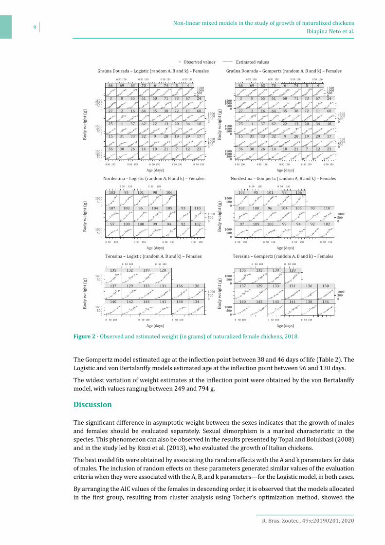
Graúna Dourada females reached the asymptotic weight at an age close to 150 days, whereas the Nordestina and Teresina females attained adult weight at approximately 200 days of age (Figures 2 and 4). The same was observed for the males (Figure 3). However, some animals of the above-mentioned ecotypes did not follow the behavior shown by the group in which they were clustered.
Negative correlation coefficients were obtained between the A and B and A and k parameters in all evaluated models, for both sexes (Table 7). The correlation coefficients obtained between the B and k parameters were positive in the evaluated models and for both sexes.
Table 6 - Estimates of parameters and evaluation criteria of the models that best described the growth of naturalized chicken ecotypes
B 3.75c 18.852 21.30b 8.082 27.35b 7.382 27.36b 7.382
k 0.0107c 7.652 0.0281b 19.072 0.0293b 16.872 0.0293b 16.872
MSE 8,265.63 5,572.70 8,199.86 8,199.68AAD 66.53 53.79 66.65 66.65R² 0.9105 0.9155 0.9308 0.9308AIC 1,416.79 1,407.34 1,758.97 1,764.97BIC 1,444.24 1,434.79 1,779.67 1,794.53MSE - mean squared error; AAD - average absolute deviation of residuals; AIC - Akaike Information Criterion; BIC - Bayesian Information Criterion.Means followed by common letters between the estimates of A, B, and k parameters in the columns do not differ significantly from each other according to the Scott-Knott test (P<0.05).1 Gompertz model: y1 = (A + u1)exp(–(B + u2)exp(–(k + u3)t)); Logistic model: y2 = (A + u1)/(1 + (B + u2)exp(–(k + u3)t)); Logistic model:
Non-linear mixed models in the study of growth of naturalized chickensIbiapina Neto et al.
9
The Gompertz model estimated age at the inflection point between 38 and 46 days of life (Table 2). The Logistic and von Bertalanffy models estimated age at the inflection point between 96 and 130 days.
The widest variation of weight estimates at the inflection point were obtained by the von Bertalanffy model, with values ranging between 249 and 794 g.
Discussion
The significant difference in asymptotic weight between the sexes indicates that the growth of males and females should be evaluated separately. Sexual dimorphism is a marked characteristic in the species. This phenomenon can also be observed in the results presented by Topal and Bolukbasi (2008) and in the study led by Rizzi et al. (2013), who evaluated the growth of Italian chickens.
The best model fits were obtained by associating the random effects with the A and k parameters for data of males. The inclusion of random effects on these parameters generated similar values of the evaluation criteria when they were associated with the A, B, and k parameters—for the Logistic model, in both cases.
By arranging the AIC values of the females in descending order, it is observed that the models allocated in the first group, resulting from cluster analysis using Tocher’s optimization method, showed the
Figure 2 - Observed and estimated weight (in grams) of naturalized female chickens, 2018.
Observed values Estimated values
Graúna Dourada – Logistic (random A, B and k) – Females Graúna Dourada – Gompertz (random A, B and k) – Females
Age (days) Age (days)50 0 15050 0 15050 0 15050 0 15050 0 15050 0 15050 0 15050
0 100
Age (days) Age (days)50 0 10050 0 10050 0 10050 0 10050 0 10050
1000500
0
1000500
0
10005000
1000500
0
1000500
0
10005000
1000500
0
1000500
0
10005000
1000500
0
1000500
0
10005000
0 15050 0 150500 15050 0 15050
0 10050 0 100500 10050 0 10050
Nordestina – Logistic (random A, B and k) – Females Nordestina – Gompertz (random A, B and k) – Females
Body
wei
ght (
g)Bo
dy w
eigh
t (g)
Teresina – Logistic (random A, B and k) – Females Teresina – Gompertz (random A, B and k) – Females
103 95 101 98 106
1109310510496108107
97 109 100 99 94 92 102
103 95 101 98 106
1109310510496108107
97 109 100 99 94 92 102
135 132 139 128
130136131133129137
140 142 143 141 138 134
135 132 139 128
130136131133129137
140 142 143 141 138 134
Body
wei
ght (
g)Bo
dy w
eigh
t (g)
Body
wei
ght (
g)
50 0 50 0 50 0 50 0 50 0 50 0 50 0 50
R. Bras. Zootec., 49:e20190201, 2020
Non-linear mixed models in the study of growth of naturalized chickensIbiapina Neto et al.
10
highest AIC values, which were higher than 7327. The second group was formed by the models with AIC values ranging from 7232 and 7152. The third group was formed by the Logistic and Gompertz models with random effect associated with the three parameters, which showed the lowest AIC values (7023.57 and 7069.48, respectively).
A similar result was observed for the clustering considering the data of males (Table 5). Group 1 contained the models with the highest AIC values, followed by groups 2, 6, 9, 7, 3, 5, 4. Lastly, group 8 included the models with the lowest AIC values.
It should be stressed that cluster analysis was processed using the values of the MSE, AAD, R2, AIC, and BIC model selection criteria, which were all considered in the formation of the groups. This is clearly observed as the AIC value of the model allocated in group 10 was between the values of the two models of group 9. Despite showing similar values for this criterion, the model of group 10 was allocated in another group because it showed different MSE and AAD values when compared with the models of group 9.
Figure 3 - Observed and estimated weight (in grams) of naturalized male chickens, 2018.
Observed values Estimated values
Graúna Dourada – Logistic (random A, B and k) – Males Graúna Dourada – Logistic (random A and k) – Males
150010005000
150010005000
15001000
5000
15001000
5000
15001000
5000
Body
wei
ght (
g)
150 0 150 150
0 150
Age (days)
47 88 87 83 82 51
39 89 41 77 90 84 86 85
79 43 57 81 42 76 80 50
59 48 91 52 75 45 53 55
56 78 58 44 54 40 46 49
Age (days)50 0 15050 0 15050 0 15050
Age (days) Age (days)
0 150
Age (days) Age (days)50 0 15050 0 15050
1000500
0
1000500
0
10005000
0 15050 0 15050
0 15050 0 15050
Nordestina – Logistic (random A, B and k) – Males Nordestina – Logistic (random A and k) – Males
Body
wei
ght (
g)
Teresina – Logistic (random A, B and k) – Males Teresina – Logistic (random A and k) – Males
120 121 119 112 125
126122114116118124
127 115 113 123 111 117
152 162 149 159
163151164155146165
157 153 166 150 145 160
Body
wei
ght (
g)Bo
dy w
eigh
t (g)
1500
1500
1500
10005000
1500
148144
158 161 147 156 154
0 15050 0 15050 0 15050
1000500
0
1000500
0
10005000
0 15050 0 15050
152 162 149 159
163151164155146165
157 153 166 150 145 160
1500
1500
1500
10005000
1500
148144
158 161 147 156 154
500 50
150010005000
150010005000
15001000
5000
15001000
5000
15001000
5000
150 0 150 150
0 150
47 88 87 83 82 51
39 89 41 77 90 84 86 85
79 43 57 81 42 76 80 50
59 48 91 52 75 45 53 55
56 78 58 44 54 40 46 49
50 0 15050 0 15050 0 15050
500 50
150010005000
15001000
5000
15001000
5000
Body
wei
ght (
g)
0 15050 0 15050 0 15050
0 15050 0 15050
120 121 119 112 125
126122114116118124
127 115 113 123 111 117
150010005000
15001000
5000
15001000
5000
Body
wei
ght (
g)
0 15050 0 15050 0 15050
0 50 0 50
R. Bras. Zootec., 49:e20190201, 2020
Non-linear mixed models in the study of growth of naturalized chickensIbiapina Neto et al.
11
The R2 values showed dissimilarity to most criteria in the choice of the best model and were thus disregarded. They did not demonstrate efficiency as a criterion for model selection. A similar trend can be observed in the results published by Sarmento et al. (2006) and Teixeira et al. (2012).
In this way, the model that best described the growth of females of the Graúna Dourada and Teresina ecotypes was the Logistic model with random effects associated with the three parameters. The Gompertz model with random effects associated with the three parameters was the one that best described the growth of Nordestina females, based on the evaluation criteria. The Gompertz model with random effect on the A and k parameters is the most suitable for the study of growth of laying hens (Galeano-Vasco et al., 2014).
The growth of Grauná Dourada and Nordestina males was best described by the Logistic model with random effects associated with the three parameters. Although the Logistic model with random effect on the A and k parameters exhibited the lowest values of the AIC and BIC criteria for the Teresina males, the AAD and MSE values were similar to those of the model with three random effects: 66.65 and 8200, respectively.
Figure 4 - Observed and estimated weight (in grams) of naturalized chickens, 2018.
Observed values Estimated values
Graúna Dourada – von Bertalanffy (random A and k) – Males Graúna Dourada – von Bertalanffy (random A and B) – Females
150010005000
150010005000
15001000
5000
15001000
5000
15001000
5000
Body
wei
ght (
g)
150 0 150 150
0 150
Age (days)
47 88 87 83 82 51
39 89 41 77 90 84 86 85
79 43 57 81 42 76 80 50
59 48 91 52 75 45 53 55
56 78 58 44 54 40 46 49
Age (days)50 0 15050 0 15050 0 15050
Body
wei
ght (
g)
500 50
150010005000
15001000
5000
15001000
5000
15001000
5000
150 0 150 150
0 15050 0 15050 0 15050 0 15050
500 50
0 15050
150010005000
150010005000
150
66 69 63 70 6 74 5 4
3 8 65 61 60 71 73 67 24
27 2 16 64 35 38 72 11 68
25 1 37 62 22 13 20 34 18
17291928932333115
36 30 26 14 10 21 7 12 23
Age (days)
0 15050 0 15050
Nordestina – von Bertalanffy (random A and k) – Males
120 121 119 112 125
126122114116118124
127 115 113 123 111 117
150010005000
15001000
5000
15001000
5000
Body
wei
ght (
g)
0 15050 0 15050 0 15050
0 150
Age (days)
50 0 15050 0 15050
1000500
0
0 15050 0 15050
Body
wei
ght (
g)
Teresina – von Bertalanffy (random A and k) – Males
152 162 149 159
163151164155146165
157 153 166 150 145 160
1500
10005000
1500
148144
158 161 147 156 154
1000500
0
1500
10005000
1500
Age (days)0 15050 0 15050 0 15050 0 15050
Age (days)
0 10050 0 10050 0 10050
1000500
0
1000500
0
10005000
1000500
0
1000500
0
10005000
0 15050 0 15050
0 10050 0 10050
Nordestina – von Bertalanffy (random A and B) – Females
Teresina – von Bertalanffy (random A and B) – Females
103 95 101 98 106
1109310510496108107
97 109 100 99 94 92 102
135 132 139 128
130136131133129137
140 142 143 141 138 134
Body
wei
ght (
g)Bo
dy w
eigh
t (g)
0 50 0 50 0 50
R. Bras. Zootec., 49:e20190201, 2020
Non-linear mixed models in the study of growth of naturalized chickensIbiapina Neto et al.
12
There was a similarity in the dispersion of residuals in the scatterplots generated with the different models. The errors observed at the beginning of the curve had a wider range for the Logistic model with the addition of three random effects, for both sexes. They were also lower at the beginning of the curve and tended to increase with age.
Residual variance estimated by MSE decreased with the addition of random effects to the model, for both sexes. Similar results showing a reduction in residual variance after the addition of random effects to the model were found by Aggrey (2009) and Karaman et al. (2013). It can thus be affirmed that the inclusion of random effects in the model may generate more-reliable estimates compared with the non-linear models of fixed effects, although the introduction of the random effect on parameter B did not lead to improvements in the estimate of the parameters.
By introducing the random effect, pointing out the difference between the individuals, individual curves are generated, as different individuals also grow differently.
Conclusions
The Teresina ecotype has the highest asymptotic weights for both sexes and is the group of slower growth when compared with the Graúna Dourada ecotype. The latter, in turn, is formed by lighter and earlier-growing animals.
Table 7 - Pearson correlation coefficients between the A, B, and k parameters, above the diagonal, and respective P-values, below the diagonal
von Bertalanffy model - FemalesA 1 −0.9817 −0.9933B 1.51 × 10⁻⁵ 1 0.9968k 7.49 × 10⁻⁷ 8.24 × 10⁻⁸ 1
R. Bras. Zootec., 49:e20190201, 2020
Non-linear mixed models in the study of growth of naturalized chickensIbiapina Neto et al.
13
The inclusion of random effects in the Logistic and Gompertz models provides greater accuracy in the estimate of the growth curve.
Conflict of Interest
The authors declare no conflict of interest.
Author Contributions
Conceptualization: V. Ibiapina Neto, F.J.V. Barbosa, J.E.G. Campelo and J.L.R. Sarmento. Data curation: V. Ibiapina Neto. Formal analysis: V. Ibiapina Neto. Funding acquisition: F.J.V. Barbosa. Investigation: V. Ibiapina Neto, F.J.V. Barbosa, J.E.G. Campelo and J.L.R. Sarmento. Methodology: V. Ibiapina Neto, F.J.V. Barbosa, J.E.G. Campelo and J.L.R. Sarmento. Project administration: V. Ibiapina Neto, F.J.V. Barbosa and J.E.G. Campelo. Resources: V. Ibiapina Neto and F.J.V. Barbosa. Software: V. Ibiapina Neto. Supervision: F.J.V. Barbosa, J.E.G. Campelo and J.L.R. Sarmento. Validation: F.J.V. Barbosa, J.E.G. Campelo and J.L.R. Sarmento. Visualization: F.J.V. Barbosa, J.E.G. Campelo and J.L.R. Sarmento. Writing-original draft: V. Ibiapina Neto. Writing-review & editing: F.J.V. Barbosa, J.E.G. Campelo and J.L.R. Sarmento.
Acknowledgments
The authors thank the Núcleo de Conservação de Galinhas Naturalizadas do Meio-Norte do Brasil (NUGAN-MN), financed by Banco do Nordeste, for the provided data.
References
Aggrey, S. E. 2009. Logistic nonlinear mixed effects model for estimating growth parameters. Poultry Science 88:276-280. https://doi.org/10.3382/ps.2008-00317
Akaike, H. 1974. A new look at the statistical model identification. IEEE Transactions on Automatic Control 19:716-723. https://doi.org/10.1109/TAC.1974.1100705
Bertalanffy, L. von. 1957. Quantitative laws in metabolism and growth. The Quarterly Review of Biology 32:217-231. https://doi.org/10.1086/401873
Galeano-Vasco, L. F.; Cerón-Muñoz, M. F. and Narváez-Solarte, W. 2014. Ability of non-linear mixed models to predict growth in laying hens. Revista Brasileira de Zootecnia 43:573-578. https://doi.org/10.1590/S1516-35982014001100003
Guedes, M. H. P.; Muniz, J. A.; Perez, J. R. O.; Silva, F. F.; Aquino, L. H. and Santos, C. L. 2004. Estudo das curvas de crescimento de cordeiros das raças Santa Inês e Bergamácia considerando heterogeneidade de variâncias. Ciência e Agrotecnologia 28:381-388. https://doi.org/10.1590/S1413-70542004000200019
Hartley, H. O. 1961. The modified Gauss-Newton method for the fitting of non-linear regression functions by least squares. Technometrics 3:269-280. https://doi.org/10.1080/00401706.1961.10489945
Hruby, M.; Hamre, M. L. and Coon, C. N. 1994. Growth modelling as a tool for predicting amino acid requirements of broilers. Journal of Applied Poultry Research 3:403-415. https://doi.org/10.1093/japr/3.4.403
Karaman, E.; Narinc, D.; Firat, M. Z. and Aksoy, T. 2013. Nonlinear mixed effects modeling of growth in Japanese quail. Poultry Science 92:1942-1948. https://doi.org/10.3382/ps.2012-02896
Laird, A. K. 1965. Dynamics of relative growth. Growth 29:249-263.
Lindstrom, M. J. and Bates, D. M. 1990. Nonlinear mixed effects models for repeated measures data. Biometrics 46:673-687. https://doi.org/10.2307/2532087
Mazucheli, J.; Souza, R. M. and Philippsen, A. S. 2011. Modelo de crescimento de Gompertz na presença de erros normais heterocedasticos: um estudo de caso. Revista Brasileira de Biometria 29:91-101.
Nelder, J. A. 1961. The fitting of a generalization of the logistic curve. Biometrics 17:89-110. https://doi.org/10.2307/2527498
R Core Team. 2017. R: A language and environment for statistical computing. R Foundation for Statistical Computing, Vienna, Austria.
Rizzi, C.; Contiero, B. and Cassandro, M. 2013. Growth patterns of Italian local chicken populations. Poultry Science 92:2226-2235. https://doi.org/10.3382/ps.2012-02825
Non-linear mixed models in the study of growth of naturalized chickensIbiapina Neto et al.
14
Romero, L. F.; Zuidhof, M. J.; Renema, R. A.; Robinson, F. E. and Naeima, A. 2009. Nonlinear mixed models to study metabolizable energy utilization in broiler breeder hens. Poultry Science 88:1310-1320. https://doi.org/10.3382/ps.2008-00102
Sarmento, J. L. R.; Rezazzi, A. J.; Souza, W. H.; Torres, R. A.; Breda, F. C. and Menezes, G. R. O. 2006. Estudo da curva de crescimento de ovinos Santa Inês. Revista Brasileira de Zootecnia 35:435-442. https://doi.org/10.1590/S1516-35982006000200014
Schwarz, G. 1978. Estimating the dimensional of a model. The Annals of Statistics 6:461-464.
Selvaggi, M.; Laudadio, V.; Dario, C. and Tufarelli, V. 2015. Modelling growth curves in a nondescript italian chicken breed: an opportunity to improve genetic and feeding strategies. The Journal of Poultry Science 52:288-294. https://doi.org/10.2141/jpsa.0150048
Sofaer, H. R.; Chapman, P. L.; Sillett, S. T. and Ghalambor, C. K. 2013. Advantages of nonlinear mixed models for fitting avian growth curves. Journal of Avian Biology 44:469-478. https://doi.org/10.1111/j.1600-048X.2013.05719.x
Strathe, A. B.; Lemme, A.; Htoo, J. K. and Kebreab, E. 2011. Estimating digestible methionine requirements for laying hens using multivariate nonlinear mixed effect models. Poultry Science 90:1496-1507. https://doi.org/10.3382/ps.2011-01345
Topal, M. and Bolukbasi, S. C. 2008. Comparison of nonlinear growth curve models in broiler chickens. Journal of Applied Animal Research 34:149-152. https://doi.org/10.1080/09712119.2008.9706960
Teixeira, M. C.; Villarroe, A. B.; Pereira, E. S.; Oliveira, S. M. P.; Albuquerque, I. A. and Mizubuti, I. Y. 2012. Curva de crescimento de cordeiros oriundos de três sistemas de produção na Região Nordeste do Brasil. Semina: Ciências Agrárias 33:2011-2018. https://doi.org/10.5433/1679-0359.2012v33n5p2011