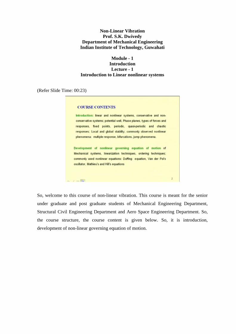
Non-Linear Vibration Prof. S.K. Dwivedy Department of Mechanical Engineering Indian Institute of Technology, Guwahati Module - 1 Introduction Lecture - 1 Introduction to Linear nonlinear systems (Refer Slide Time: 00:23) So, welcome to this course of non-linear vibration. This course is meant for the senior under graduate and post graduate students of Mechanical Engineering Department, Structural Civil Engineering Department and Aero Space Engineering Department. So, the course structure, the course content is given below. So, it is introduction, development of non-linear governing equation of motion.
Transcript
Non-Linear Vibration Prof. S.K. Dwivedy
Department of Mechanical Engineering Indian Institute of Technology, Guwahati
Module - 1
Introduction Lecture - 1
Introduction to Linear nonlinear systems
(Refer Slide Time: 00:23)
So, welcome to this course of non-linear vibration. This course is meant for the senior
under graduate and post graduate students of Mechanical Engineering Department,
Structural Civil Engineering Department and Aero Space Engineering Department. So,
the course structure, the course content is given below. So, it is introduction,
development of non-linear governing equation of motion.
(Refer Slide Time: 00:46)
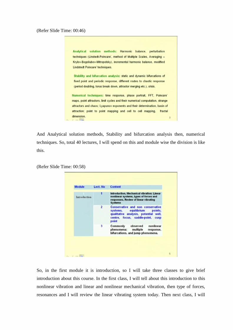
And Analytical solution methods, Stability and bifurcation analysis then, numerical
techniques. So, total 40 lectures, I will spend on this and module wise the division is like
this.
(Refer Slide Time: 00:58)
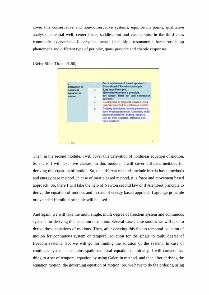
So, in the first module it is introduction, so I will take three classes to give brief
introduction about this course. In the first class, I will tell about this introduction to this
nonlinear vibration and linear and nonlinear mechanical vibration, then type of forces,
resonances and I will review the linear vibrating system today. Then next class, I will
cover this conservative and non-conservative systems, equilibrium points, qualitative
analysis, potential well, center focus, saddle-point and cusp points. In the third class
commonly observed non-linear phenomena like multiple resonance, bifurcations, jump
phenomena and different type of periodic, quasi periodic and chaotic responses.
(Refer Slide Time: 01:50)
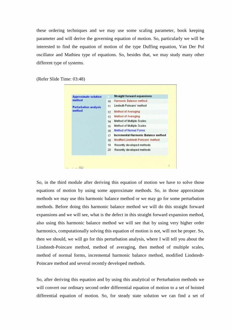
Then, in the second module, I will cover this derivation of nonlinear equation of motion.
So there, I will take five classes; in this module, I will cover different methods for
deriving this equation of motion. So, the different methods include inertia based methods
and energy base method. In case of inertia based method, it is force and movement based
approach. So, there I will take the help of Newton second law or d’Alembert principle to
derive the equation of motion, and in case of energy based approach Lagrange principle
or extended Hamilton principle will be used.
And again, we will take the multi single, multi degree of freedom system and continuous
systems for deriving this equation of motion. Several cases, case studies we will take to
derive these equations of motions. Then, after deriving this Spatio temporal equation of
motion for continuous system or temporal equation for the single to multi degree of
freedom systems. So, we will go for finding the solution of the system. In case of
continues system, it contains spatio temporal equation or initially, I will convert that
thing to a set of temporal equation by using Galerkin method, and then after deriving the
equation motion, the governing equation of motion. So, we have to do the ordering using
these ordering techniques and we may use some scaling parameter, book keeping
parameter and will derive the governing equation of motion. So, particularly we will be
interested to find the equation of motion of the type Duffing equation, Van Der Pol
oscillator and Mathieu type of equations. So, besides that, we may study many other
different type of systems.
(Refer Slide Time: 03:48)
So, in the third module after deriving this equation of motion we have to solve those
equations of motion by using some approximate methods. So, in those approximate
methods we may use this harmonic balance method or we may go for some perturbation
methods. Before doing this harmonic balance method we will do this straight forward
expansions and we will see, what is the defect in this straight forward expansion method,
also using this harmonic balance method we will see that by using very higher order
harmonics, computationally solving this equation of motion is not, will not be proper. So,
then we should, we will go for this perturbation analysis, where I will tell you about the
Lindstedt-Poincare method, method of averaging, then method of multiple scales,
method of normal forms, incremental harmonic balance method, modified Lindstedt-
Poincare method and several recently developed methods.
So, after deriving this equation and by using this analytical or Perturbation methods we
will convert our ordinary second order differential equation of motion to a set of hoisted
differential equation of motion. So, for steady state solution we can find a set of
algebraic equations, which we can numerically solve to find the response of the system.
Then, we will be interested to see the equilibrium, the equilibrium response, equilibrium
points and their stability.
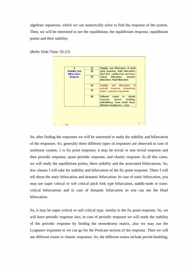
(Refer Slide Time: 05:23)
So, after finding the responses we will be interested to study the stability and bifurcation
of the responses. So, generally three different types of responses are observed in case of
nonlinear system, 1 is fix point response; it may be trivial or non trivial response and
then periodic response, quasi periodic response, and chaotic response. In all this cases,
we will study the equilibrium points, there stability and the associated bifurcations. So,
few classes I will take for stability and bifurcation of the fix point response. There I will
tell about the static bifurcation and dynamic bifurcation. In case of static bifurcation, you
may see super critical or soft critical pitch fork type bifurcation, saddle-node or trans-
critical bifurcations and in case of dynamic bifurcation so you can see the Hopf
bifurcation.
So, it may be super critical or soft critical type, similar to the fix point response. So, we
will have periodic response also, in case of periodic response we will study the stability
of the periodic response by finding the monodromy matrix, also we may use the
Lyapunov exponent or we can go for the Poincare section of the response. Then we will
see different routes to chaotic responses. So, the different routes include period doubling,
intermittency, torus break down, attractor merging and we will also study about the crisis
observed in case of the chaotic responses.
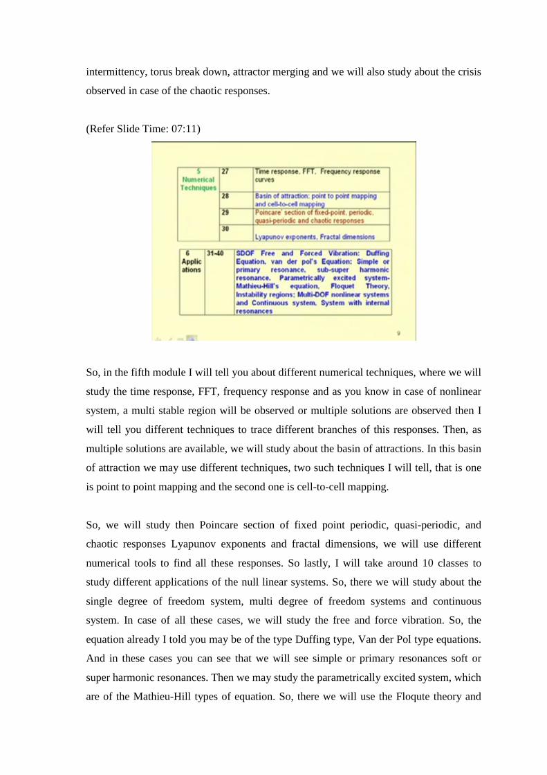
(Refer Slide Time: 07:11)
So, in the fifth module I will tell you about different numerical techniques, where we will
study the time response, FFT, frequency response and as you know in case of nonlinear
system, a multi stable region will be observed or multiple solutions are observed then I
will tell you different techniques to trace different branches of this responses. Then, as
multiple solutions are available, we will study about the basin of attractions. In this basin
of attraction we may use different techniques, two such techniques I will tell, that is one
is point to point mapping and the second one is cell-to-cell mapping.
So, we will study then Poincare section of fixed point periodic, quasi-periodic, and
chaotic responses Lyapunov exponents and fractal dimensions, we will use different
numerical tools to find all these responses. So lastly, I will take around 10 classes to
study different applications of the null linear systems. So, there we will study about the
single degree of freedom system, multi degree of freedom systems and continuous
system. In case of all these cases, we will study the free and force vibration. So, the
equation already I told you may be of the type Duffing type, Van der Pol type equations.
And in these cases you can see that we will see simple or primary resonances soft or
super harmonic resonances. Then we may study the parametrically excited system, which
are of the Mathieu-Hill types of equation. So, there we will use the Floqute theory and
we can study the instability region and some cases of internal resonances also will be
covered in this course.
(Refer Slide Time: 09:18)
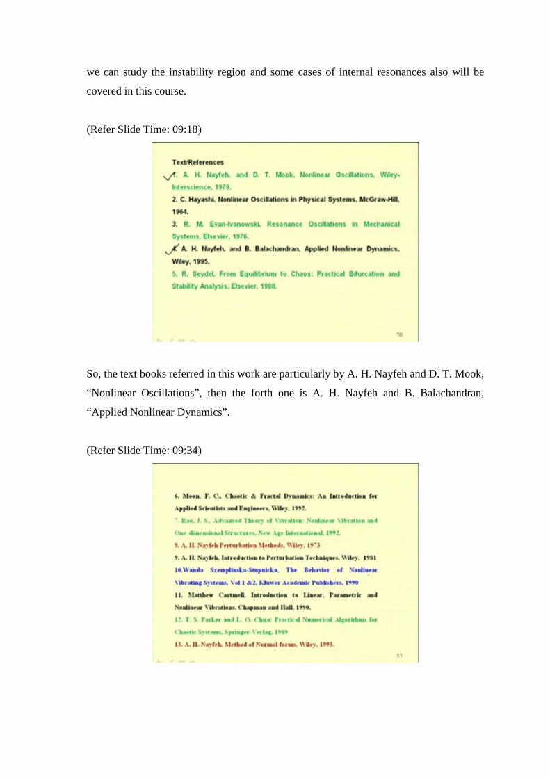
So, the text books referred in this work are particularly by A. H. Nayfeh and D. T. Mook,
“Nonlinear Oscillations”, then the forth one is A. H. Nayfeh and B. Balachandran,
“Applied Nonlinear Dynamics”.
(Refer Slide Time: 09:34)
Also the other references I will follow that is by Moon F. C., “Chaotic and Fractal
Dynamics: An Introduction for Applied Scientists and Engineers”, then “Perturbation
Methods” by Nayfeh, then “Introduction to Perturbation Techniques” by Nayfeh, then
“The Behavior of Nonlinear Vibrating System” by Wanda Szemplinska-Stupnika,
“Introduction to Linear Parametric and Nonlinear Vibrations” by Cartmell and “Practical
Numerical Algorithms for Chaotic Systems” by Parker and Chua. Also, I will give you
few examples and the method of normal forms there I will use the book by A. H. Nayfeh.
(Refer Slide Time: 10:20)
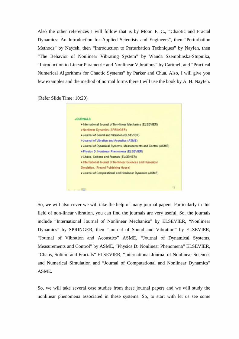
So, we will also cover we will take the help of many journal papers. Particularly in this
field of non-linear vibration, you can find the journals are very useful. So, the journals
include “International Journal of Nonlinear Mechanics” by ELSEVIER, “Nonlinear
Dynamics” by SPRINGER, then “Journal of Sound and Vibration” by ELSEVIER,
“Journal of Vibration and Acoustics” ASME, “Journal of Dynamical Systems,
Measurements and Control” by ASME, “Physics D: Nonlinear Phenomena” ELSEVIER,
“Chaos, Soliton and Fractals” ELSEVIER, “International Journal of Nonlinear Sciences
and Numerical Simulation and “Journal of Computational and Nonlinear Dynamics”
ASME.
So, we will take several case studies from these journal papers and we will study the
nonlinear phenomena associated in these systems. So, to start with let us see some
mechanical systems and we will see how the vibration phenomenon is occurring in those
systems.
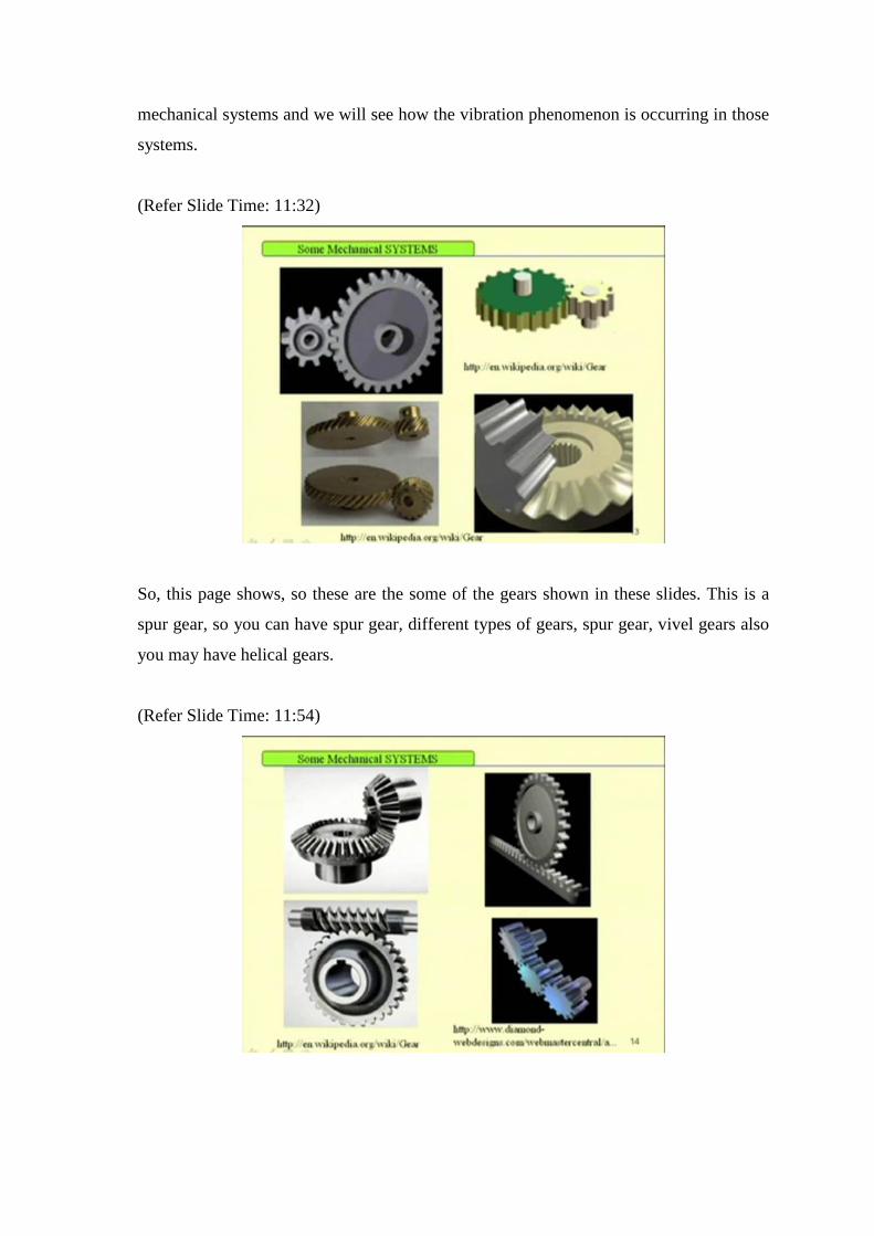
(Refer Slide Time: 11:32)
So, this page shows, so these are the some of the gears shown in these slides. This is a
spur gear, so you can have spur gear, different types of gears, spur gear, vivel gears also
you may have helical gears.
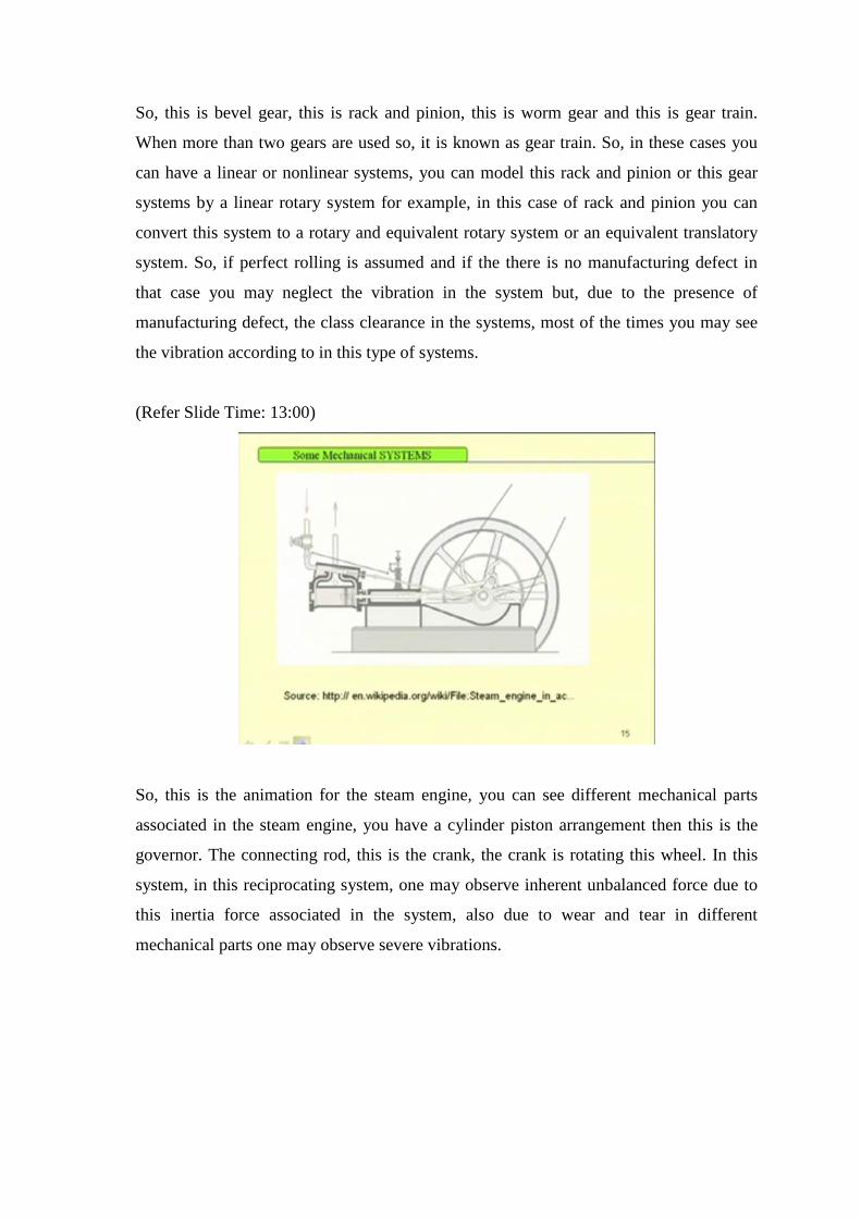
(Refer Slide Time: 11:54)
So, this is bevel gear, this is rack and pinion, this is worm gear and this is gear train.
When more than two gears are used so, it is known as gear train. So, in these cases you
can have a linear or nonlinear systems, you can model this rack and pinion or this gear
systems by a linear rotary system for example, in this case of rack and pinion you can
convert this system to a rotary and equivalent rotary system or an equivalent translatory
system. So, if perfect rolling is assumed and if the there is no manufacturing defect in
that case you may neglect the vibration in the system but, due to the presence of
manufacturing defect, the class clearance in the systems, most of the times you may see
the vibration according to in this type of systems.
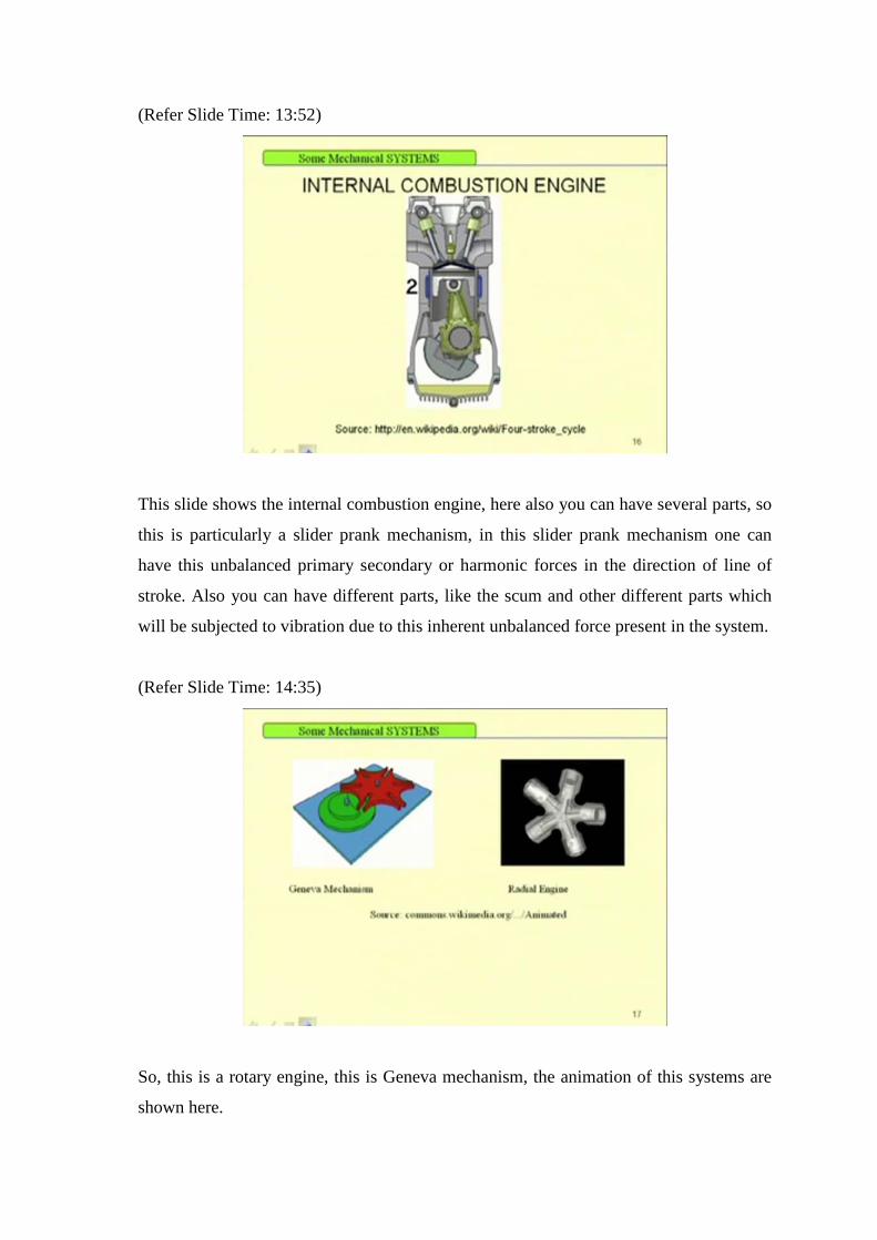
(Refer Slide Time: 13:00)
So, this is the animation for the steam engine, you can see different mechanical parts
associated in the steam engine, you have a cylinder piston arrangement then this is the
governor. The connecting rod, this is the crank, the crank is rotating this wheel. In this
system, in this reciprocating system, one may observe inherent unbalanced force due to
this inertia force associated in the system, also due to wear and tear in different
mechanical parts one may observe severe vibrations.
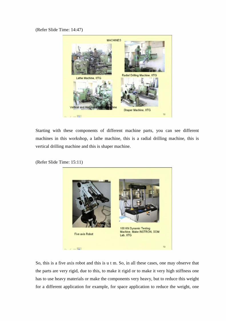
(Refer Slide Time: 13:52)
This slide shows the internal combustion engine, here also you can have several parts, so
this is particularly a slider prank mechanism, in this slider prank mechanism one can
have this unbalanced primary secondary or harmonic forces in the direction of line of
stroke. Also you can have different parts, like the scum and other different parts which
will be subjected to vibration due to this inherent unbalanced force present in the system.
(Refer Slide Time: 14:35)
So, this is a rotary engine, this is Geneva mechanism, the animation of this systems are
shown here.
(Refer Slide Time: 14:47)
Starting with these components of different machine parts, you can see different
machines in this workshop, a lathe machine, this is a radial drilling machine, this is
vertical drilling machine and this is shaper machine.
(Refer Slide Time: 15:11)
So, this is a five axis robot and this is u t m. So, in all these cases, one may observe that
the parts are very rigid, due to this, to make it rigid or to make it very high stiffness one
has to use heavy materials or make the components very heavy, but to reduce this weight
for a different application for example, for space application to reduce the weight, one
has to use light or flexible material. So, in case of flexible or light material the
components will be subjected to vibration.
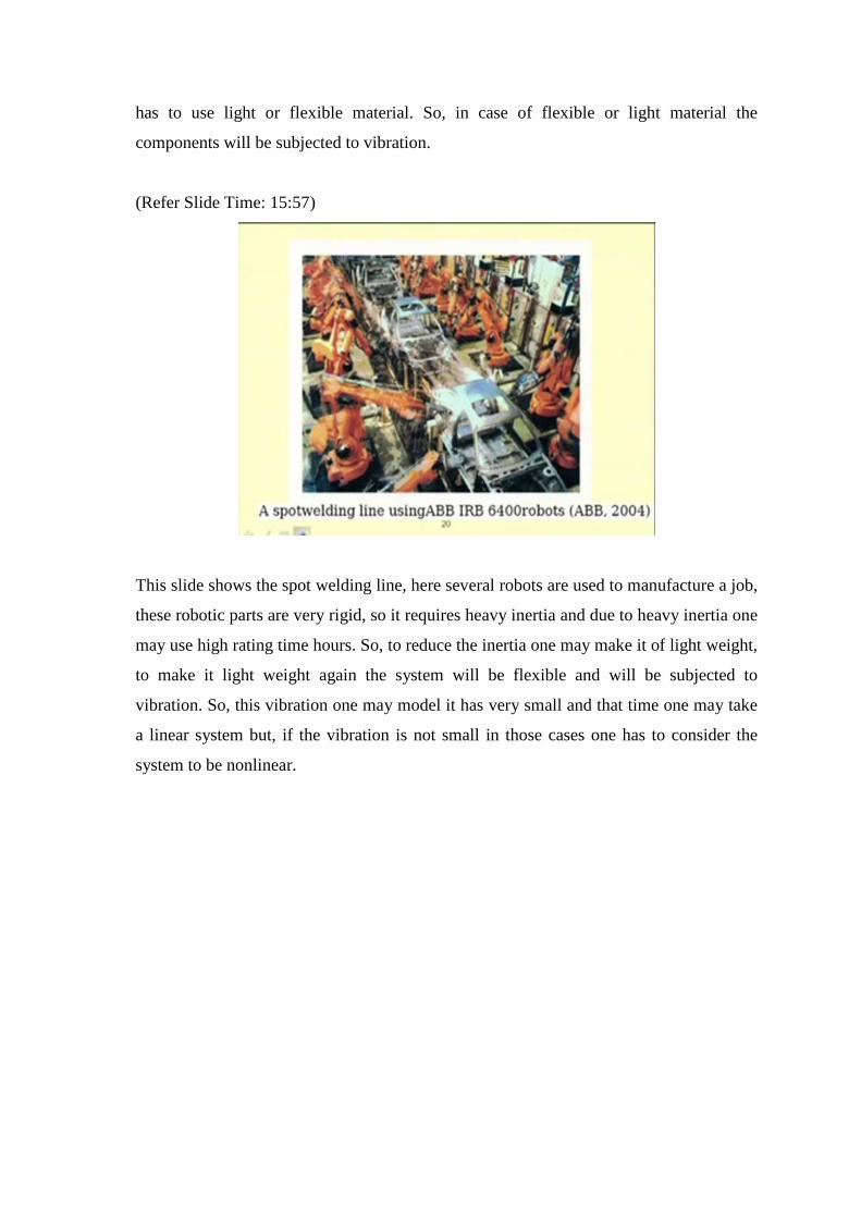
(Refer Slide Time: 15:57)
This slide shows the spot welding line, here several robots are used to manufacture a job,
these robotic parts are very rigid, so it requires heavy inertia and due to heavy inertia one
may use high rating time hours. So, to reduce the inertia one may make it of light weight,
to make it light weight again the system will be flexible and will be subjected to
vibration. So, this vibration one may model it has very small and that time one may take
a linear system but, if the vibration is not small in those cases one has to consider the
system to be nonlinear.
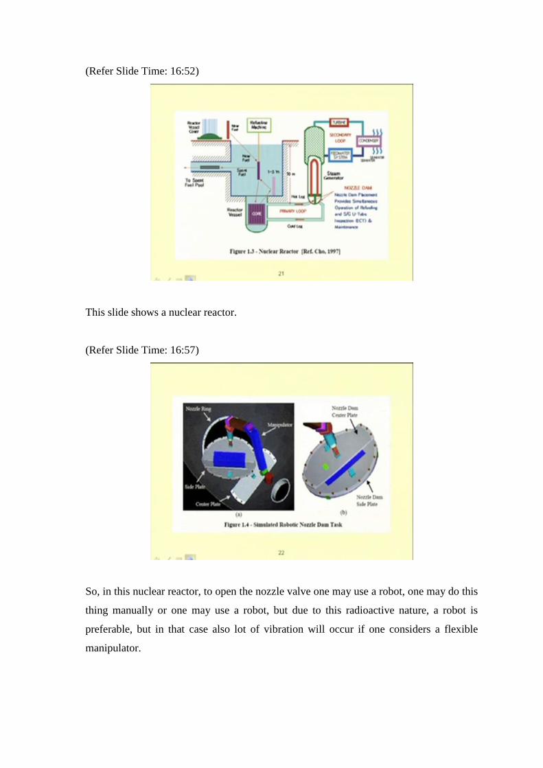
(Refer Slide Time: 16:52)
This slide shows a nuclear reactor.
(Refer Slide Time: 16:57)
So, in this nuclear reactor, to open the nozzle valve one may use a robot, one may do this
thing manually or one may use a robot, but due to this radioactive nature, a robot is
preferable, but in that case also lot of vibration will occur if one considers a flexible
manipulator.
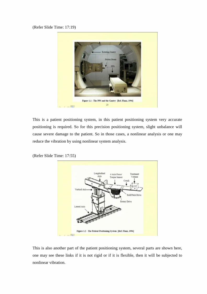
(Refer Slide Time: 17:19)
This is a patient positioning system, in this patient positioning system very accurate
positioning is required. So for this precision positioning system, slight unbalance will
cause severe damage to the patient. So in those cases, a nonlinear analysis or one may
reduce the vibration by using nonlinear system analysis.
(Refer Slide Time: 17:55)
This is also another part of the patient positioning system, several parts are shown here,
one may see these links if it is not rigid or if it is flexible, then it will be subjected to
nonlinear vibration.
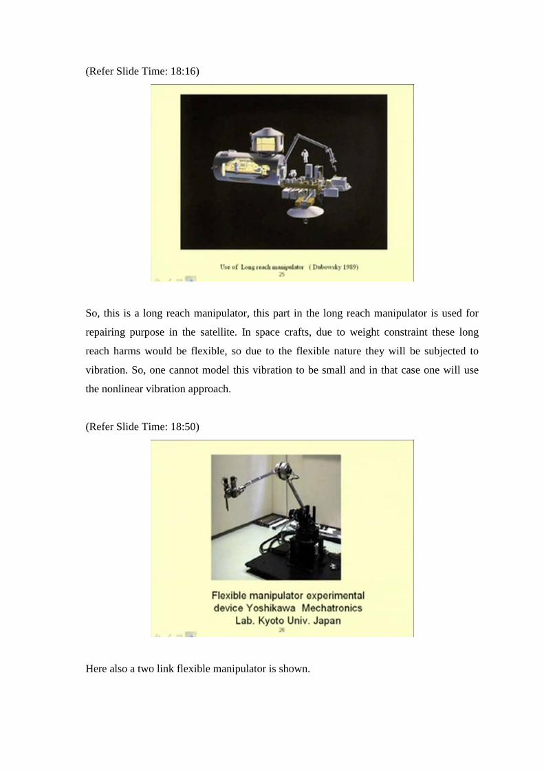
(Refer Slide Time: 18:16)
So, this is a long reach manipulator, this part in the long reach manipulator is used for
repairing purpose in the satellite. In space crafts, due to weight constraint these long
reach harms would be flexible, so due to the flexible nature they will be subjected to
vibration. So, one cannot model this vibration to be small and in that case one will use
the nonlinear vibration approach.
(Refer Slide Time: 18:50)
Here also a two link flexible manipulator is shown.
(Refer Slide Time: 18:57)
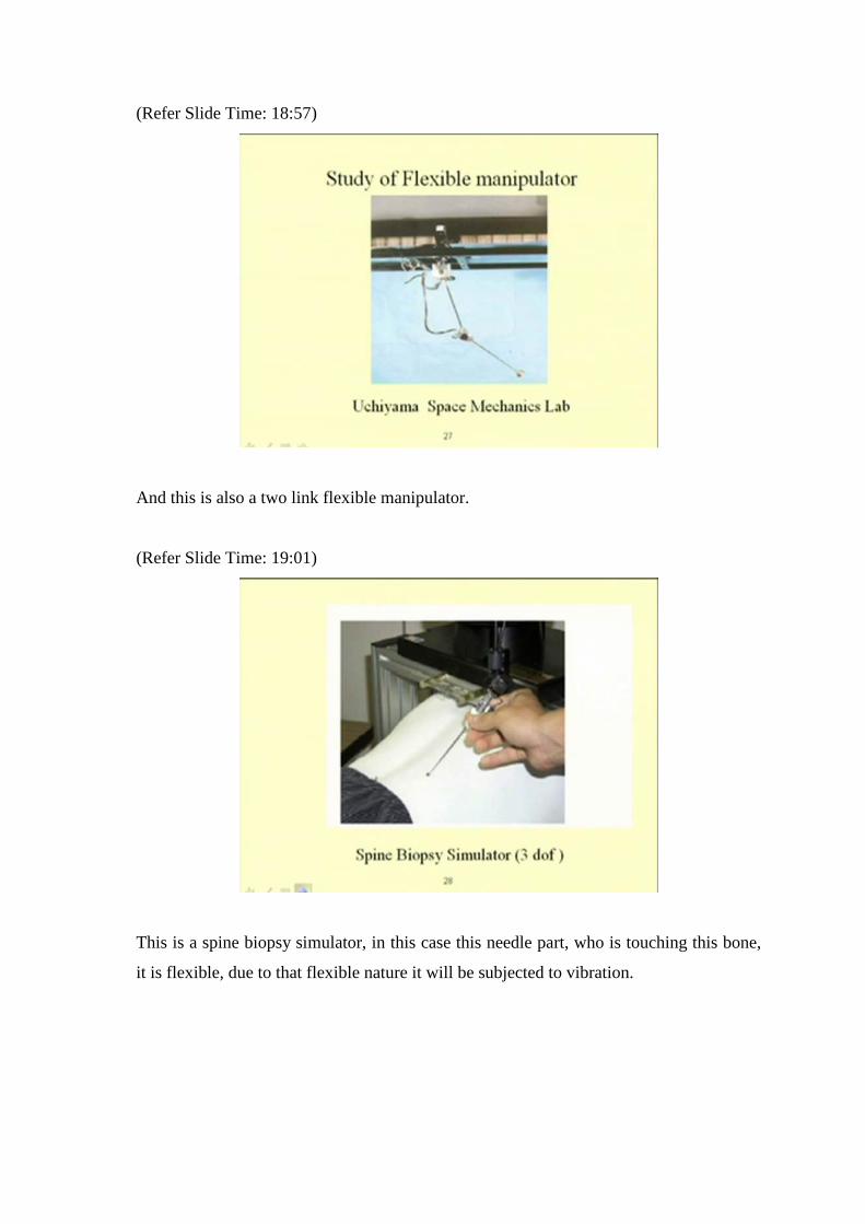
And this is also a two link flexible manipulator.
(Refer Slide Time: 19:01)
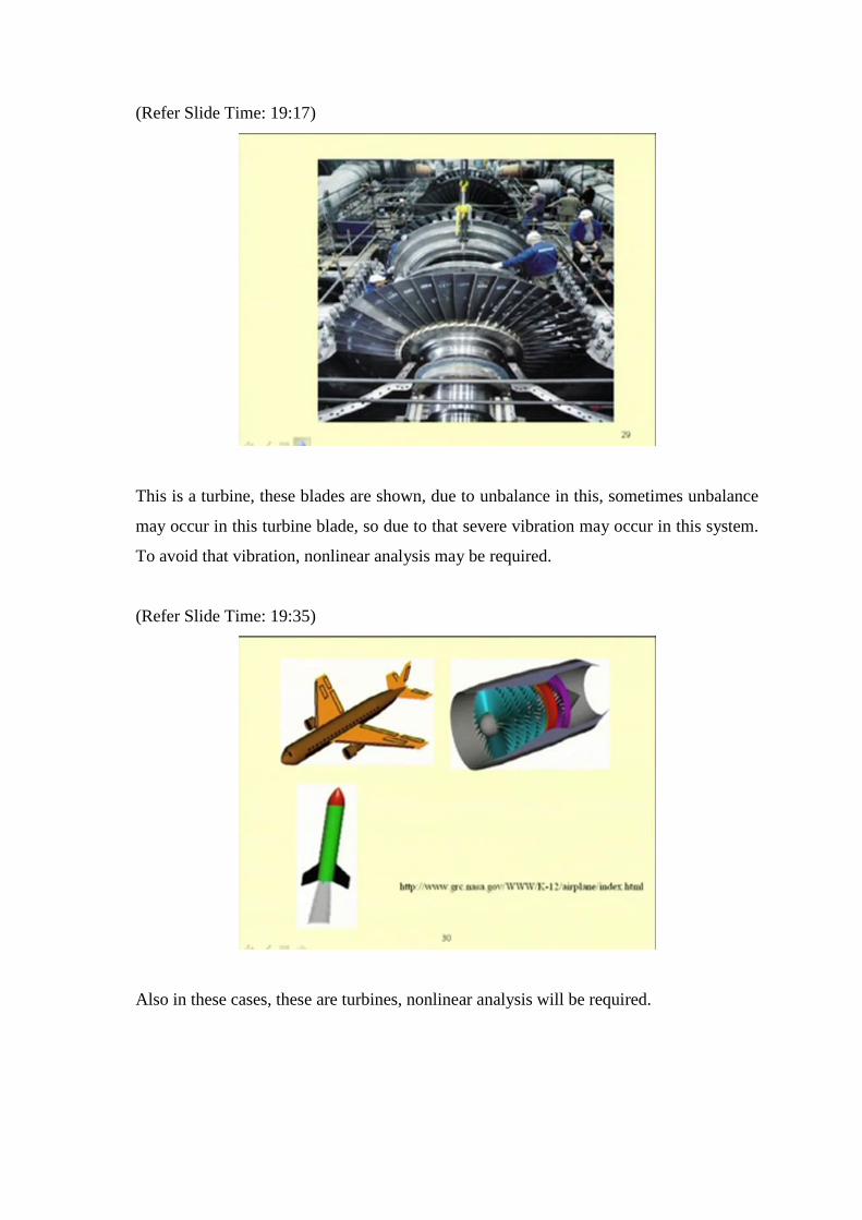
This is a spine biopsy simulator, in this case this needle part, who is touching this bone,
it is flexible, due to that flexible nature it will be subjected to vibration.
(Refer Slide Time: 19:17)
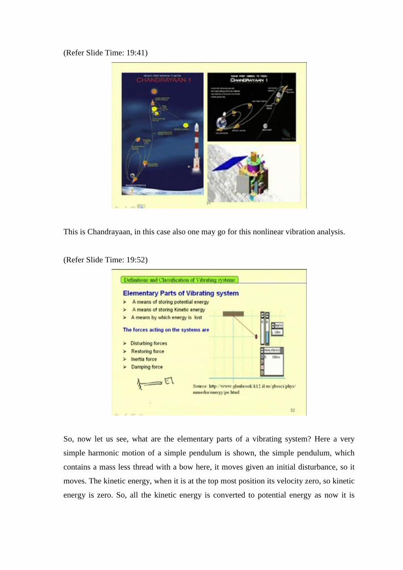
This is a turbine, these blades are shown, due to unbalance in this, sometimes unbalance
may occur in this turbine blade, so due to that severe vibration may occur in this system.
To avoid that vibration, nonlinear analysis may be required.
(Refer Slide Time: 19:35)
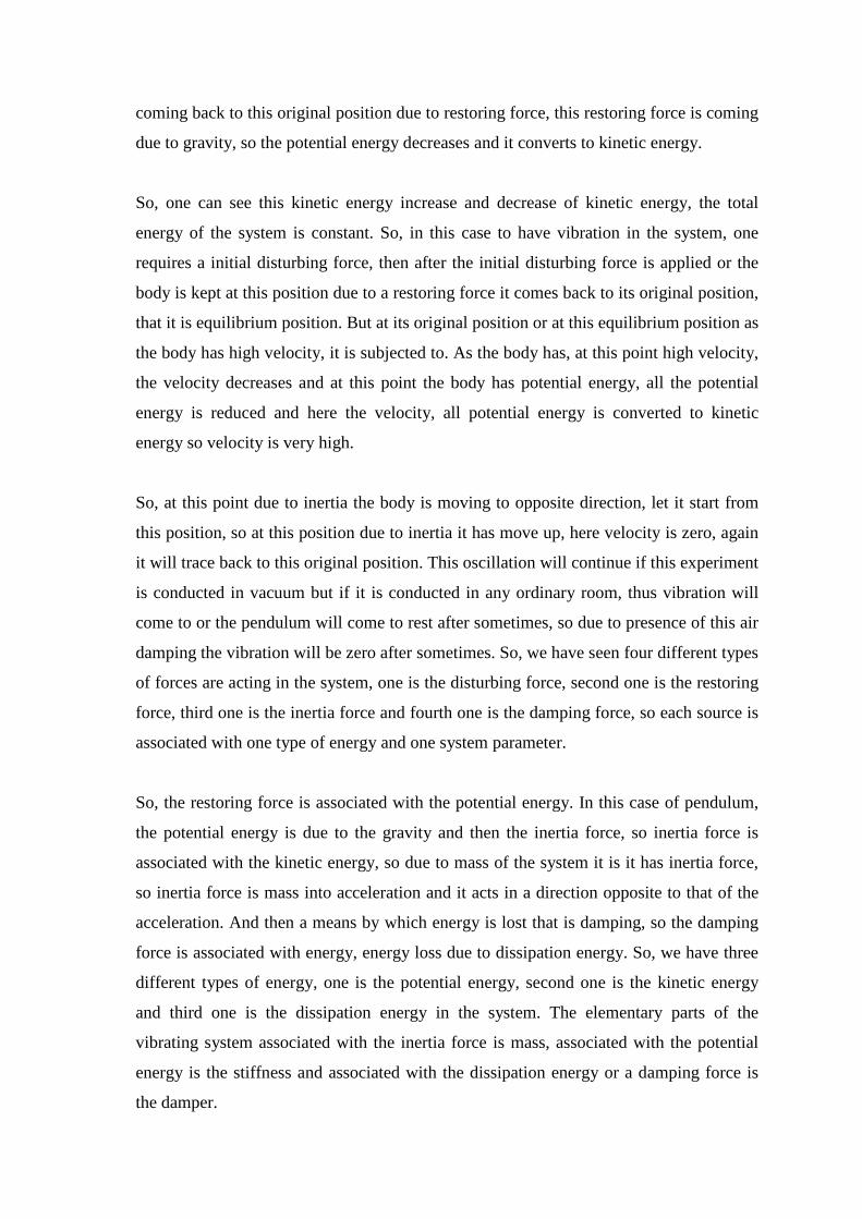
Also in these cases, these are turbines, nonlinear analysis will be required.
(Refer Slide Time: 19:41)
This is Chandrayaan, in this case also one may go for this nonlinear vibration analysis.
(Refer Slide Time: 19:52)
So, now let us see, what are the elementary parts of a vibrating system? Here a very
simple harmonic motion of a simple pendulum is shown, the simple pendulum, which
contains a mass less thread with a bow here, it moves given an initial disturbance, so it
moves. The kinetic energy, when it is at the top most position its velocity zero, so kinetic
energy is zero. So, all the kinetic energy is converted to potential energy as now it is
coming back to this original position due to restoring force, this restoring force is coming
due to gravity, so the potential energy decreases and it converts to kinetic energy.
So, one can see this kinetic energy increase and decrease of kinetic energy, the total
energy of the system is constant. So, in this case to have vibration in the system, one
requires a initial disturbing force, then after the initial disturbing force is applied or the
body is kept at this position due to a restoring force it comes back to its original position,
that it is equilibrium position. But at its original position or at this equilibrium position as
the body has high velocity, it is subjected to. As the body has, at this point high velocity,
the velocity decreases and at this point the body has potential energy, all the potential
energy is reduced and here the velocity, all potential energy is converted to kinetic
energy so velocity is very high.
So, at this point due to inertia the body is moving to opposite direction, let it start from
this position, so at this position due to inertia it has move up, here velocity is zero, again
it will trace back to this original position. This oscillation will continue if this experiment
is conducted in vacuum but if it is conducted in any ordinary room, thus vibration will
come to or the pendulum will come to rest after sometimes, so due to presence of this air
damping the vibration will be zero after sometimes. So, we have seen four different types
of forces are acting in the system, one is the disturbing force, second one is the restoring
force, third one is the inertia force and fourth one is the damping force, so each source is
associated with one type of energy and one system parameter.
So, the restoring force is associated with the potential energy. In this case of pendulum,
the potential energy is due to the gravity and then the inertia force, so inertia force is
associated with the kinetic energy, so due to mass of the system it is it has inertia force,
so inertia force is mass into acceleration and it acts in a direction opposite to that of the
acceleration. And then a means by which energy is lost that is damping, so the damping
force is associated with energy, energy loss due to dissipation energy. So, we have three
different types of energy, one is the potential energy, second one is the kinetic energy
and third one is the dissipation energy in the system. The elementary parts of the
vibrating system associated with the inertia force is mass, associated with the potential
energy is the stiffness and associated with the dissipation energy or a damping force is
the damper.
So, in a system one may use a mass, a stiffness and a damping element. So in case of the
stiffness for example, in this case due to this gravity, so it has gained this potential
energy. But if one will take a cantilever beam or a beam so in that case, due to the
elasticity of the system, elasticity E of the system, EI of the system, the body will gain
this potential energy or the potential energy will be the strain energy in this case. So a
vibrating system will have a mass, a spring element or a stiffness element then a
damping element.
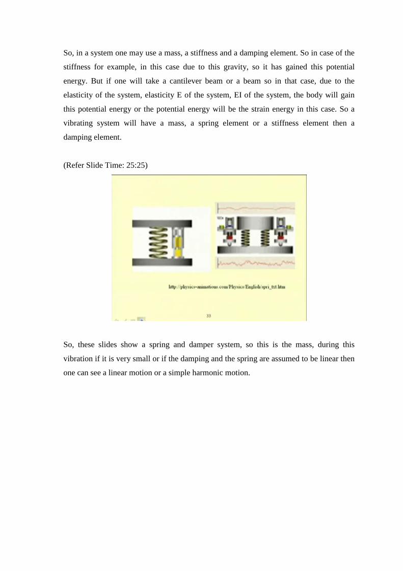
(Refer Slide Time: 25:25)
So, these slides show a spring and damper system, so this is the mass, during this
vibration if it is very small or if the damping and the spring are assumed to be linear then
one can see a linear motion or a simple harmonic motion.
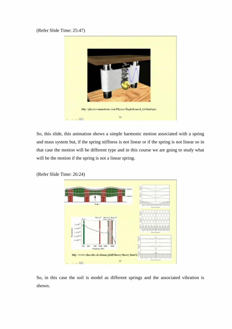
(Refer Slide Time: 25:47)
So, this slide, this animation shows a simple harmonic motion associated with a spring
and mass system but, if the spring stiffness is not linear or if the spring is not linear so in
that case the motion will be different type and in this course we are going to study what
will be the motion if the spring is not a linear spring.
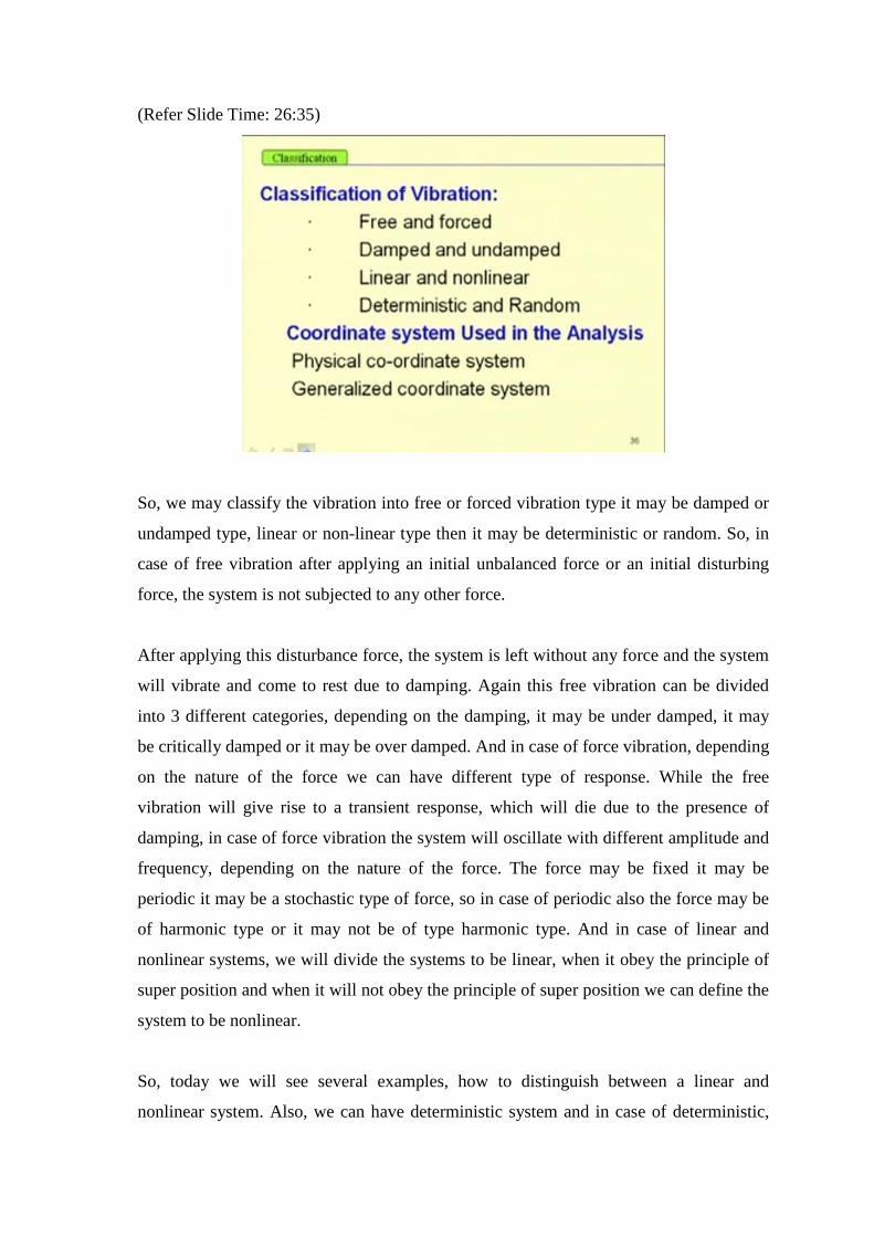
(Refer Slide Time: 26:24)
So, in this case the soil is model as different springs and the associated vibration is
shown.
(Refer Slide Time: 26:35)
So, we may classify the vibration into free or forced vibration type it may be damped or
undamped type, linear or non-linear type then it may be deterministic or random. So, in
case of free vibration after applying an initial unbalanced force or an initial disturbing
force, the system is not subjected to any other force.
After applying this disturbance force, the system is left without any force and the system
will vibrate and come to rest due to damping. Again this free vibration can be divided
into 3 different categories, depending on the damping, it may be under damped, it may
be critically damped or it may be over damped. And in case of force vibration, depending
on the nature of the force we can have different type of response. While the free
vibration will give rise to a transient response, which will die due to the presence of
damping, in case of force vibration the system will oscillate with different amplitude and
frequency, depending on the nature of the force. The force may be fixed it may be
periodic it may be a stochastic type of force, so in case of periodic also the force may be
of harmonic type or it may not be of type harmonic type. And in case of linear and
nonlinear systems, we will divide the systems to be linear, when it obey the principle of
super position and when it will not obey the principle of super position we can define the
system to be nonlinear.
So, today we will see several examples, how to distinguish between a linear and
nonlinear system. Also, we can have deterministic system and in case of deterministic,
we may have in case of deterministic response, we may have fix point response the
response may be periodic, it may be quasi periodic or it may be chaotic. And the force
may be a random type of force, the force may be a deterministic type of force also. The
earth quake force is a random type of force, so in all these cases to analyze the system we
required different coordinate systems.
The coordinate system maybe a physical coordinate system or it may be a generalized
coordinate system. That thing we will discuss more in second module. So, one may
follow 4 different steps for this vibration analysis.
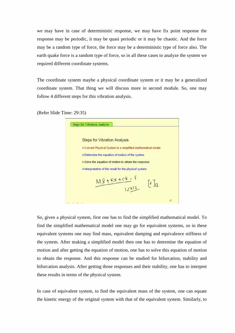
(Refer Slide Time: 29:35)
So, given a physical system, first one has to find the simplified mathematical model. To
find the simplified mathematical model one may go for equivalent systems, so in these
equivalent systems one may find mass, equivalent damping and equivalence stiffness of
the system. After making a simplified model then one has to determine the equation of
motion and after getting the equation of motion, one has to solve this equation of motion
to obtain the response. And this response can be studied for bifurcation, stability and
bifurcation analysis. After getting those responses and their stability, one has to interpret
these results in terms of the physical system.
In case of equivalent system, to find the equivalent mass of the system, one can equate
the kinetic energy of the original system with that of the equivalent system. Similarly, to
find the equivalent stiffness of the system, the potential energy of the original system
would be equated with the potential energy of the equivalent system and in case of
equivalent damping, one has to equate the dissipation energy of the original system with
that of the equivalent system. We will see some examples, how to find this equivalent
mass, stiffness and damping. And to model or to get simplified model, one can use this
lumped parameter system, one can model the system as a single degree of freedom
system two degree of freedom system or multi degree of freedom system or one can go
for a continuous system modeling also. In case of single, two or multi degree of freedom
system, one will have a one will have. In case of single degree of freedom system, one
will have single differential equation of motion. In case of two degree of freedom system
one will have a matrix equation differential equation in this form, that is M x double dot
plus K x plus C x dot equal to F. So, in this mass M is the mass matrix, K is the stiffness
matrix, C is the damping matrix, x is the response and F is the force applied to the
system.
So, F is a vector and x is a vector. In case of multi degree of freedom system, one has to
solve this. If this is a n degree of freedom system for example, one can take a 12 storey
building, so in that case one can write this a matrix by using a 12 is to 12 element.
Similarly, the stiffness and damping matrix can be written with 12 is to 12 elements, and
this force will be at F vector, so it will contain 12 components. So, one can use model
reduction method or model analysis to convert this equation, if this equation, if this mass
matrix and stiffness matrix and damping matrix are coupled, then one can use this model
analysis method to convert these equations or to convert this mass matrix, stiffness
matrix and damping matrix to a set of uncoupled differential equation of motion.
So, in that way by using model analysis method, one can have n number of uncoupled
single degree of freedom equation. So, knowing the solution of a single degree of
freedom system, one can find the response of a multi degree of freedom system also.
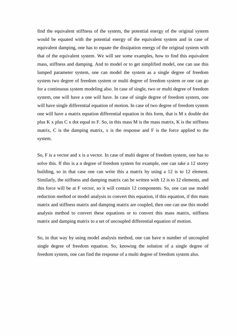
(Refer Slide Time: 33:51)
So, here several examples are given, this is only a spring and dumber. The equation of
motion can be written as, K x plus C x dot equal to F, so this is a first order system. In
this case, this is a spring, mass and damper system, the equation of motion can be written
as M x double dot, where x is the displacement of this, so M x double dot plus K x plus
C x dot equal to F, so this is a second order system. So, in these cases I am assuming the
spring to be linear, that is why the spring force or the stiffness force I am writing equal to
K x but, if the spring is not linear then one cannot write this spring force to be K x and in
that case the equation of motion will be nonlinear.
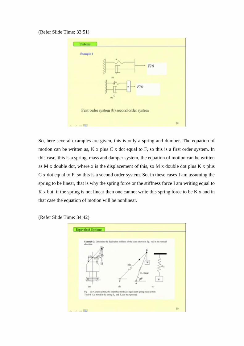
(Refer Slide Time: 34:42)
So, to find equivalent stiffness, for example, let us take this crane system. In this crane
system, this rod and this beam, so one can find the equivalent spring for this one and
finally, as it is moving in this direction, the mass is moving in the downward direction,
so, one can find one equivalent stiffness of the system.
So, as this rod is subjected to axial force then one can find the strain energy associated in
this axial direction, one can find the strain energy here and for these two elements and
then equate to that of the equivalent spring.
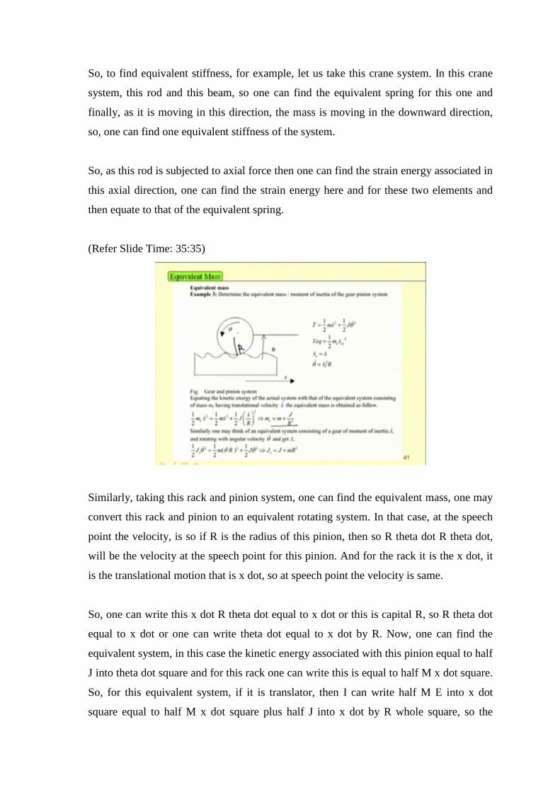
(Refer Slide Time: 35:35)
Similarly, taking this rack and pinion system, one can find the equivalent mass, one may
convert this rack and pinion to an equivalent rotating system. In that case, at the speech
point the velocity, is so if R is the radius of this pinion, then so R theta dot R theta dot,
will be the velocity at the speech point for this pinion. And for the rack it is the x dot, it
is the translational motion that is x dot, so at speech point the velocity is same.
So, one can write this x dot R theta dot equal to x dot or this is capital R, so R theta dot
equal to x dot or one can write theta dot equal to x dot by R. Now, one can find the
equivalent system, in this case the kinetic energy associated with this pinion equal to half
J into theta dot square and for this rack one can write this is equal to half M x dot square.
So, for this equivalent system, if it is translator, then I can write half M E into x dot
square equal to half M x dot square plus half J into x dot by R whole square, so the
equivalent mass becomes M plus J by R square. Similarly, one can convert this thing,
this whole system to an equivalent translatory system.
So, in that case, in case of equivalent translatory system the mass is this. In case of
equivalent rotary system one can find the inertia associated with the system, so
equivalent inertia equal to J plus M R square. So similarly, by equating the dissipation
energy one can find the equivalent damping or equivalent viscous damping of the
system.
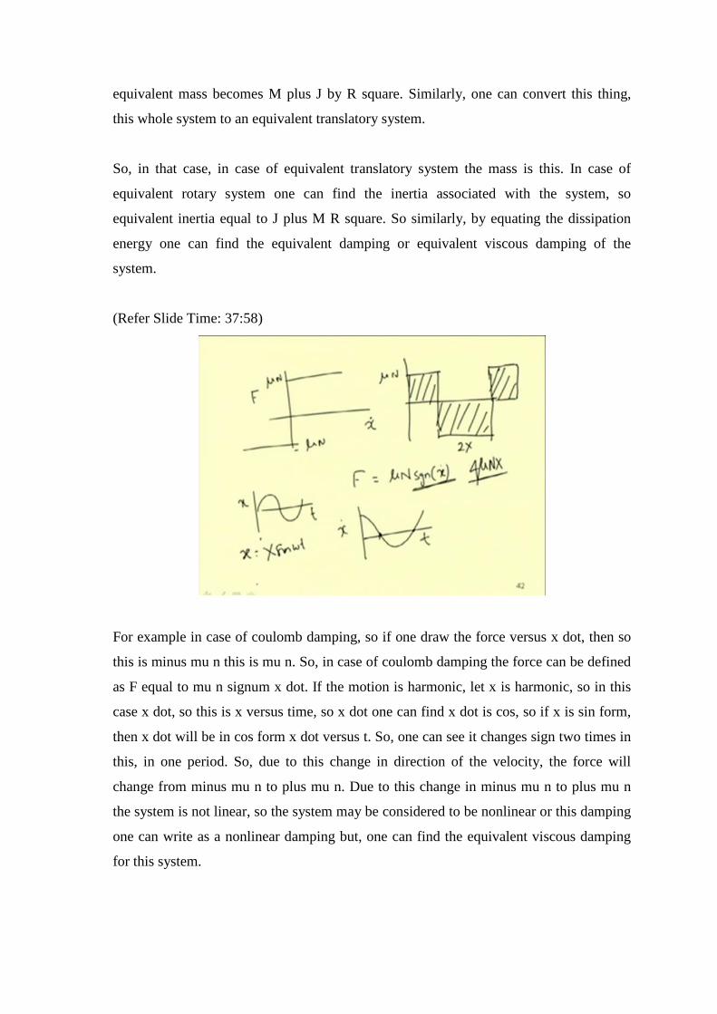
(Refer Slide Time: 37:58)
For example in case of coulomb damping, so if one draw the force versus x dot, then so
this is minus mu n this is mu n. So, in case of coulomb damping the force can be defined
as F equal to mu n signum x dot. If the motion is harmonic, let x is harmonic, so in this
case x dot, so this is x versus time, so x dot one can find x dot is cos, so if x is sin form,
then x dot will be in cos form x dot versus t. So, one can see it changes sign two times in
this, in one period. So, due to this change in direction of the velocity, the force will
change from minus mu n to plus mu n. Due to this change in minus mu n to plus mu n
the system is not linear, so the system may be considered to be nonlinear or this damping
one can write as a nonlinear damping but, one can find the equivalent viscous damping
for this system.
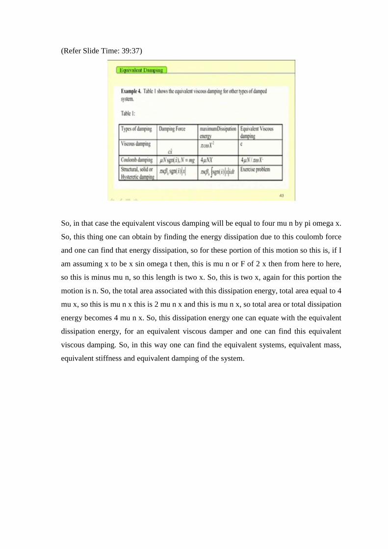
(Refer Slide Time: 39:37)
So, in that case the equivalent viscous damping will be equal to four mu n by pi omega x.
So, this thing one can obtain by finding the energy dissipation due to this coulomb force
and one can find that energy dissipation, so for these portion of this motion so this is, if I
am assuming x to be x sin omega t then, this is mu n or F of 2 x then from here to here,
so this is minus mu n, so this length is two x. So, this is two x, again for this portion the
motion is n. So, the total area associated with this dissipation energy, total area equal to 4
mu x, so this is mu n x this is 2 mu n x and this is mu n x, so total area or total dissipation
energy becomes 4 mu n x. So, this dissipation energy one can equate with the equivalent
dissipation energy, for an equivalent viscous damper and one can find this equivalent
viscous damping. So, in this way one can find the equivalent systems, equivalent mass,
equivalent stiffness and equivalent damping of the system.
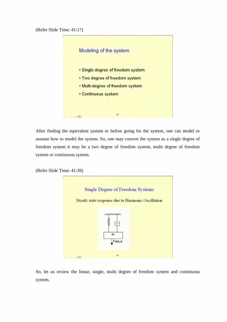
(Refer Slide Time: 41:17)
After finding the equivalent system or before going for the system, one can model or
assume how to model the system. So, one may convert the system as a single degree of
freedom system it may be a two degree of freedom system, multi degree of freedom
system or continuous system.
(Refer Slide Time: 41:39)
So, let us review the linear, single, multi degree of freedom system and continuous
system.
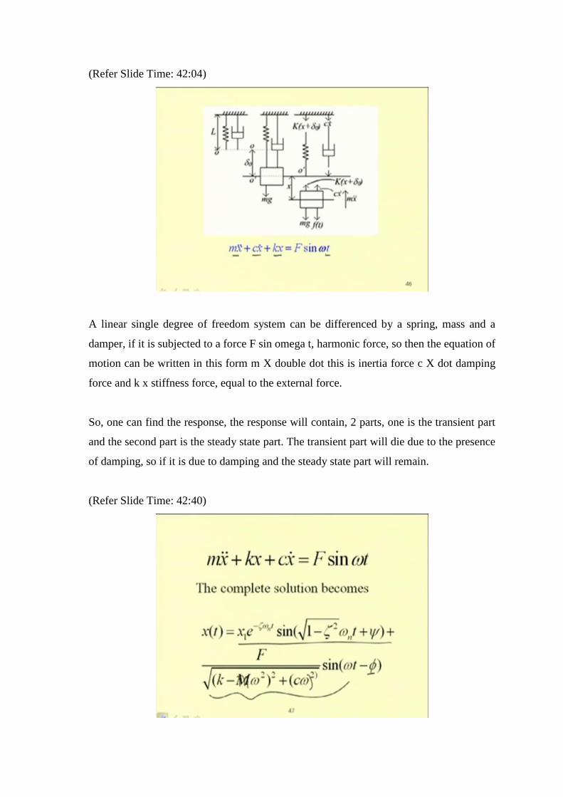
(Refer Slide Time: 42:04)
A linear single degree of freedom system can be differenced by a spring, mass and a
damper, if it is subjected to a force F sin omega t, harmonic force, so then the equation of
motion can be written in this form m X double dot this is inertia force c X dot damping
force and k x stiffness force, equal to the external force.
So, one can find the response, the response will contain, 2 parts, one is the transient part
and the second part is the steady state part. The transient part will die due to the presence
of damping, so if it is due to damping and the steady state part will remain.
(Refer Slide Time: 42:40)
So, the total solution of the system, equal to x one e to the power minus zeta omega n t
sin one minus zeta square omega n t plus psi plus F by root over k minus M omega
square, so this is small m, m omega square whole square plus c omega whole square.
So, in this case the first part is the transient part and the second part is the steady state
response of the system, the transient part, this x one and psi depend on the initial
condition and phi is the phase difference, this phase difference will give the time lag of
or the time after which the response will occur when a force is applied to the system. So,
we can have a rotating system the force we have applied in this system depending on
different systems.
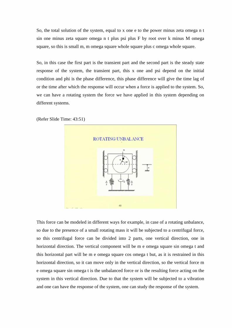
(Refer Slide Time: 43:51)
This force can be modeled in different ways for example, in case of a rotating unbalance,
so due to the presence of a small rotating mass it will be subjected to a centrifugal force,
so this centrifugal force can be divided into 2 parts, one vertical direction, one in
horizontal direction. The vertical component will be m e omega square sin omega t and
this horizontal part will be m e omega square cos omega t but, as it is restrained in this
horizontal direction, so it can move only in the vertical direction, so the vertical force m
e omega square sin omega t is the unbalanced force or is the resulting force acting on the
system in this vertical direction. Due to that the system will be subjected to a vibration
and one can have the response of the system, one can study the response of the system.
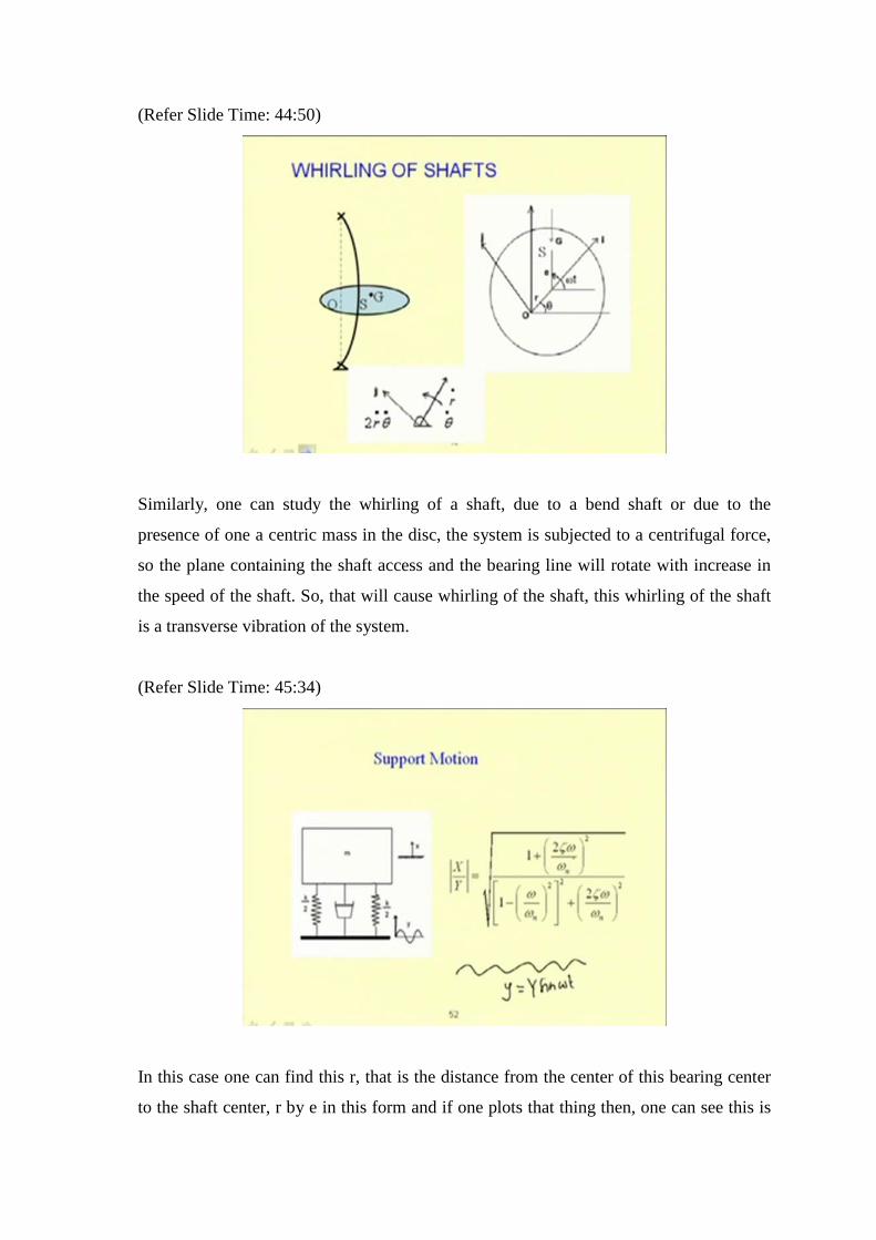
(Refer Slide Time: 44:50)
Similarly, one can study the whirling of a shaft, due to a bend shaft or due to the
presence of one a centric mass in the disc, the system is subjected to a centrifugal force,
so the plane containing the shaft access and the bearing line will rotate with increase in
the speed of the shaft. So, that will cause whirling of the shaft, this whirling of the shaft
is a transverse vibration of the system.
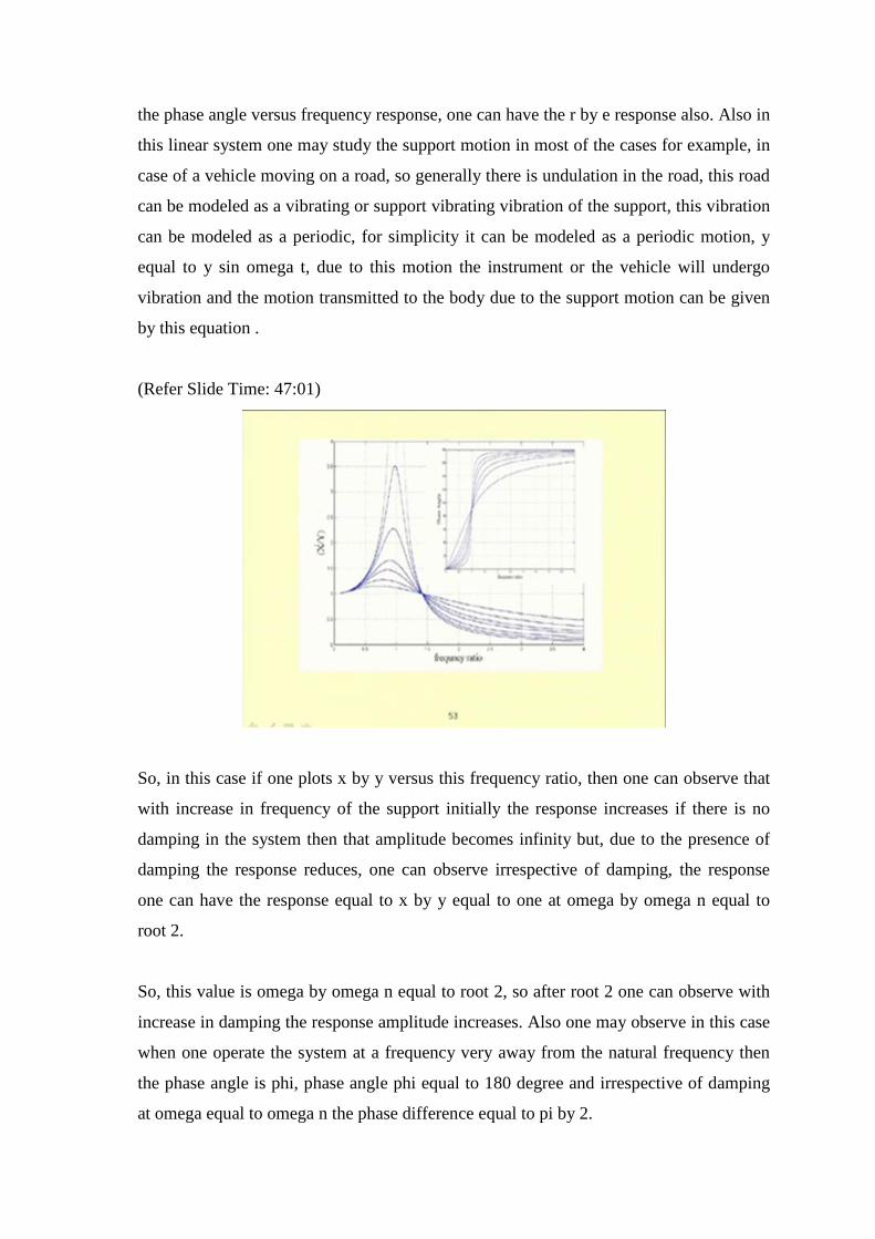
(Refer Slide Time: 45:34)
In this case one can find this r, that is the distance from the center of this bearing center
to the shaft center, r by e in this form and if one plots that thing then, one can see this is
the phase angle versus frequency response, one can have the r by e response also. Also in
this linear system one may study the support motion in most of the cases for example, in
case of a vehicle moving on a road, so generally there is undulation in the road, this road
can be modeled as a vibrating or support vibrating vibration of the support, this vibration
can be modeled as a periodic, for simplicity it can be modeled as a periodic motion, y
equal to y sin omega t, due to this motion the instrument or the vehicle will undergo
vibration and the motion transmitted to the body due to the support motion can be given
by this equation .
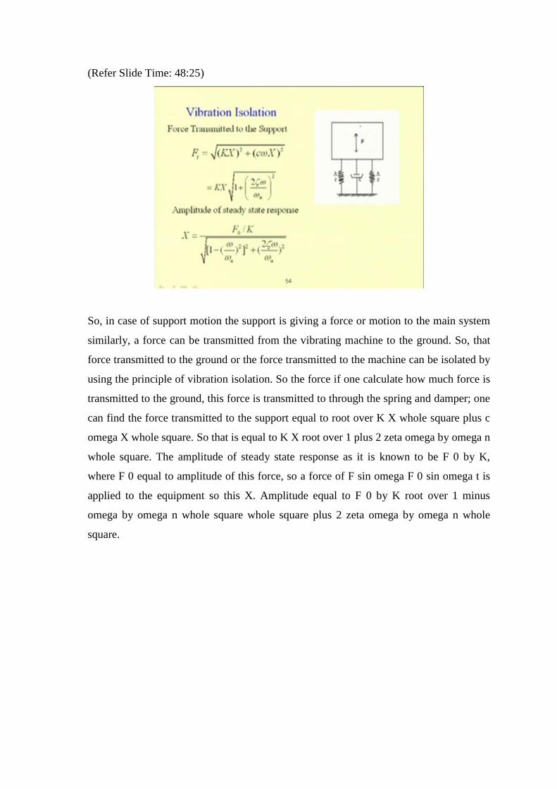
(Refer Slide Time: 47:01)
So, in this case if one plots x by y versus this frequency ratio, then one can observe that
with increase in frequency of the support initially the response increases if there is no
damping in the system then that amplitude becomes infinity but, due to the presence of
damping the response reduces, one can observe irrespective of damping, the response
one can have the response equal to x by y equal to one at omega by omega n equal to
root 2.
So, this value is omega by omega n equal to root 2, so after root 2 one can observe with
increase in damping the response amplitude increases. Also one may observe in this case
when one operate the system at a frequency very away from the natural frequency then
the phase angle is phi, phase angle phi equal to 180 degree and irrespective of damping
at omega equal to omega n the phase difference equal to pi by 2.
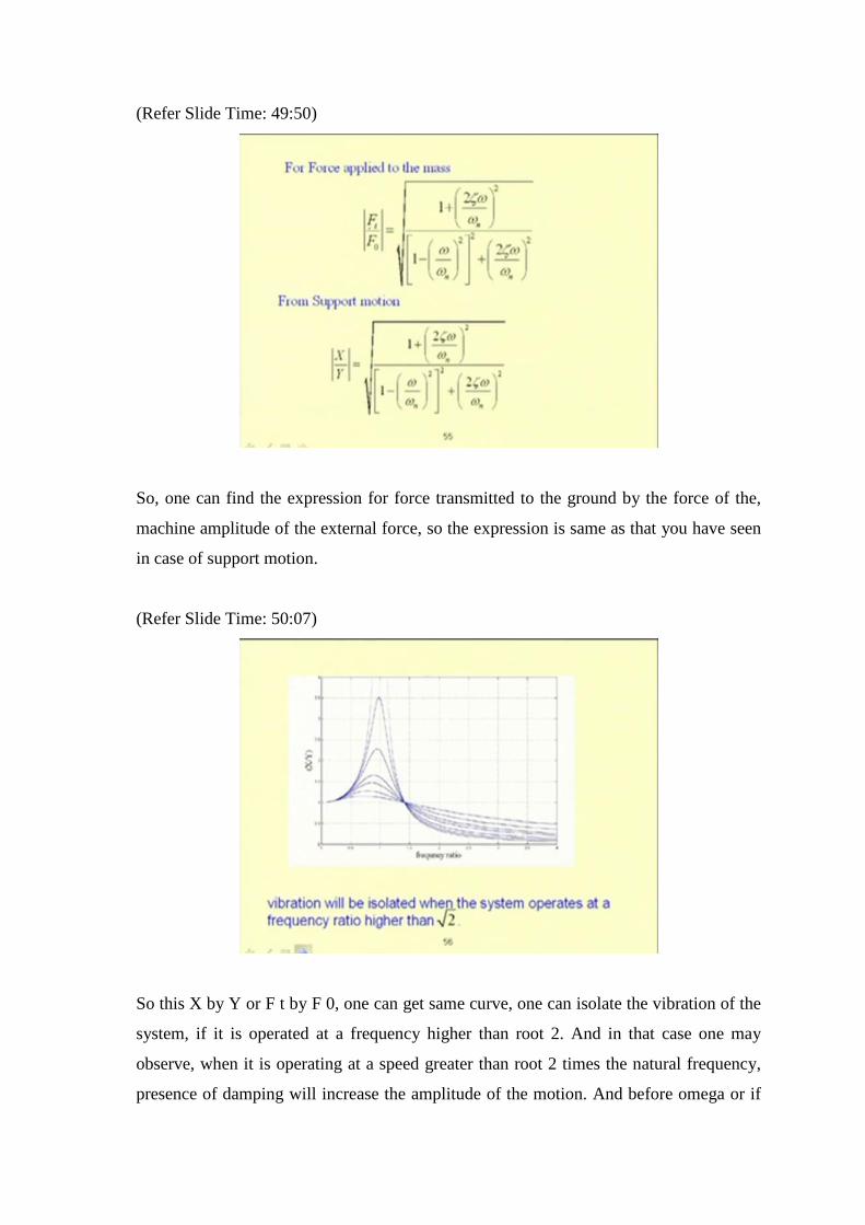
(Refer Slide Time: 48:25)
So, in case of support motion the support is giving a force or motion to the main system
similarly, a force can be transmitted from the vibrating machine to the ground. So, that
force transmitted to the ground or the force transmitted to the machine can be isolated by
using the principle of vibration isolation. So the force if one calculate how much force is
transmitted to the ground, this force is transmitted to through the spring and damper; one
can find the force transmitted to the support equal to root over K X whole square plus c
omega X whole square. So that is equal to K X root over 1 plus 2 zeta omega by omega n
whole square. The amplitude of steady state response as it is known to be F 0 by K,
where F 0 equal to amplitude of this force, so a force of F sin omega F 0 sin omega t is
applied to the equipment so this X. Amplitude equal to F 0 by K root over 1 minus
omega by omega n whole square whole square plus 2 zeta omega by omega n whole
square.
(Refer Slide Time: 49:50)
So, one can find the expression for force transmitted to the ground by the force of the,
machine amplitude of the external force, so the expression is same as that you have seen
in case of support motion.
(Refer Slide Time: 50:07)
So this X by Y or F t by F 0, one can get same curve, one can isolate the vibration of the
system, if it is operated at a frequency higher than root 2. And in that case one may
observe, when it is operating at a speed greater than root 2 times the natural frequency,
presence of damping will increase the amplitude of the motion. And before omega or if
omega is less than the natural frequency, omega is the external frequency, if the external
frequency is less than the natural frequency of the system, then a damper is a must. So, if
there is no damping, so when one increase the frequency of the system, it reaches a
frequency, it reaches a very high value of amplitude, it may be infinity at omega equal to
omega n if there is no damping present in the system.
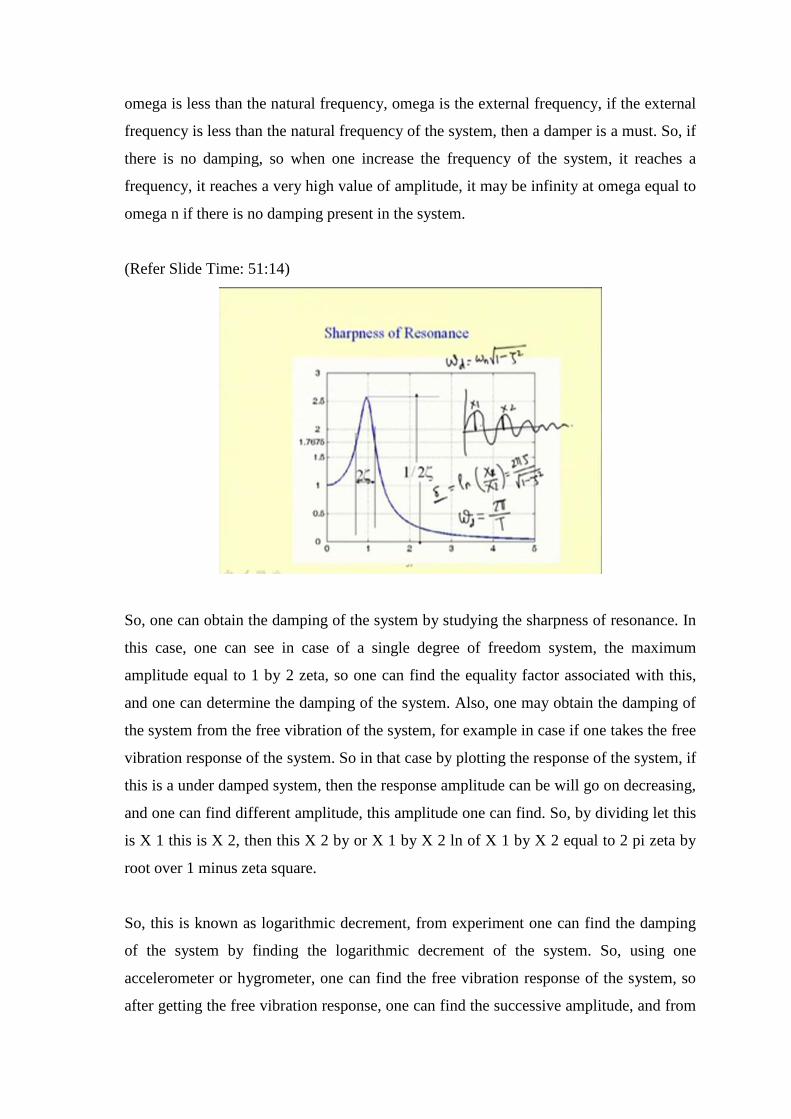
(Refer Slide Time: 51:14)
So, one can obtain the damping of the system by studying the sharpness of resonance. In
this case, one can see in case of a single degree of freedom system, the maximum
amplitude equal to 1 by 2 zeta, so one can find the equality factor associated with this,
and one can determine the damping of the system. Also, one may obtain the damping of
the system from the free vibration of the system, for example in case if one takes the free
vibration response of the system. So in that case by plotting the response of the system, if
this is a under damped system, then the response amplitude can be will go on decreasing,
and one can find different amplitude, this amplitude one can find. So, by dividing let this
is X 1 this is X 2, then this X 2 by or X 1 by X 2 ln of X 1 by X 2 equal to 2 pi zeta by
root over 1 minus zeta square.
So, this is known as logarithmic decrement, from experiment one can find the damping
of the system by finding the logarithmic decrement of the system. So, using one
accelerometer or hygrometer, one can find the free vibration response of the system, so
after getting the free vibration response, one can find the successive amplitude, and from
that one can obtain the logarithmic decrement of the system. After getting logarithmic
decrement of the system, one can find damping of the system. So if the damping is very
small, one can neglect this zeta square with respect to 1, so one can write this logarithmic
decrement equal to 2 pi zeta and one can easily get zeta from that.
Also, from this time response one can find the time period, one can find this omega d,
that is damp natural frequency of the system, equal to 2 pi by t, if one get the time period
of the system then one can find this omega d. So, the natural frequency of the system as
it is related to the damp natural frequency by the expression omega d equal to omega n
into root over 1 minus zeta square, one can obtain omega n of the system. After getting
the natural frequency one can find the system parameter or system stiffness, if mass of
the system is known. So from the vibration response of this linear system, one can find
or identify the system parameters.
One may use this vibration measuring instruments, which work on same principle as that
of the support motion to manufacture this vibration measuring instrument. So, recalling
this X by Y or Z by Y, Z is the relative motion, one can use the same system as a
accelerometer when it is operating at a very low frequency and use as a seismometer
when it is operated at a very high frequency. So today’s class we have studied about the
or we have reviewed the linear system, we know different types of nonlinear systems,
and also we have seen the application of the course that is the nonlinear vibration system
to a range of systems.
So, this course will be useful for the senior undergraduate or post graduate students in
Mechanical Engineering Department, Civil Structural or Aerospace Engineering
Department. So in the next class, we will see the difference between linear and nonlinear
systems and we will also study the different phenomena associated with the nonlinear