Non-Parallelizable Real Projective Space and

Stiefel-Whitney Classes

See-Hak Seong

November 14, 2016

Abstract

Parallelizability allows us to define a collection of continuous vector fields on a manifold which forms a basis onevery tangent space. Therefore, many properties of tangent spaces of a manifold can be easily discovered byobserving this collection of vector fields. However, mathematicians find out that S2 is not parallelizable and

mathematicians need to decide whether an arbitrary manifold is parallelizable or not. In this paper, I will suggestone method that many mathematicians used in order to conclude non-parallelizability, named Stiefel-Whitney

Classes, and I will show you how it works on real projective spaces RPn.

0. Preliminaries

In this part, I will briefly state all basic definitions of smooth manifolds and smooth functions. In order to defineparallelizablity, we need to define vector bundle and tangent bundle which will be handled in the next section. Sincesmooth manifolds and their tangent manifolds are usual examples of vector bundle and tangent bundle, this partwill help you to construct intuition of bundles.

Definition 0.1. A be any index set. R-vector space RA is defined by RA :� tx | x : AÑ R is a functionu. Forany α P A, define α-th coordinate of x by the value xpαq and denote it as xα. For any function f : Y Ñ RA, definefαpyq :� α-th coordinate of fpyq.

Example 0.2. For A � t1, 2, � � � , nu, RA is denoted by Rn. And for arbitrary function f : Y Ñ Rn, f can beinterpreted as f � pf1, � � � , fnq.

Definition 0.3. (Smooth functions on Rn) For an open subset U � Rn, a function f : U ÑM � RA is called

smooth if fα : U Ñ R is C8 for all α P A. In this case, pBf

Buiqα �

BfαBui

.

Note. In some papers, the word ‘map’ is used instead of ‘continuous function’.

Definition 0.4. (Smooth manifolds) A subset M � RA is called a smooth manifold of dimension n ¥ 0 if forany x PM , there exists an open set U P Rn and a smooth function h : U Ñ RA which satisfy following properties :(a) There exists a neighborhood V of x in M such that h : U Ñ V is a homeomorphism.

(b) For all u P U , the matrix rBhαpuq

Bujs has rank n.

In this case, V � hpUq is called as coordinate neighborhood in M , and triple pU, V, hq is called as local parametriza-tion of M .

Note. In some book(Boothby) a local parametrization pU, V, hq is expressed in another way by using its inverse.In this case, the inverse h�1 : V Ñ U � Rn is defined as local coordinate system or chart for M . However, in thispaper I will define local coordinate system differently in the next section.

Definition 0.5. (Tangent vector, space, manifold) A vector v P RA is tangent to M at a point x PM if v canbe defined as the velocity vector of some smooth path in M that passes x. The collection of those tangent vectors

1

is defiend as tangent space of M at x and denoted by DMx. Moreover, the collection of those tangent spaces withtheir standard points is defined as tangent manifold and denoted as DM .

DM :� tpx, vq PM � RA | v P DMxu

Definition 0.6. (Smooth functions on a manifold) M � RA and N � RB are smooth manifolds. Let’s takea point x0 P M with a local parametrization pU, V, hq of M with x0 � hpu0q. The function f : M Ñ N is saidto be smooth at x0 if f � h : U Ñ N � RB is smooth on some neighborhood of u0. If f is smooth at all pointsinM , then f is called smooth. Moreover, f is called a diffeomorphism if f is bijective and both f and f�1 are smooth.

Remark. With all of definitions above, we can construct the category of smooth manifolds and smooth maps.Although we need to show several things more, such as whether composition of smooth functions is smooth, sinceall those things can be proved easily I will just claim that this collection of smooth manifolds and smooth functionssatisfies category structure. So if we consider with this category, diffeomorphism can be explained as an isomor-phism between two objects in this category.

1. Vector Bundles

Basic idea of vector bundles comes from attaching arbitrary real vector spaces at each point of a topologicalspace. Although this idea sounds weird, the intuitive example of vector bundle is always suggested in calculusclasses in different way, namely tangent space of a sphere. If we recall this example, then we could possibly guessthat concept of vector bundle is a generalization of a collection of tangent spaces labelled with each standard points.With this intuition, I will state the definition of vector bundles, tangent bundles, and parallelizability of topologicalspaces. Moreover, several properties and methods to create new vector bundles will be suggested in this section inorder to prepare for the next section.

Note. Among all part of this paper I will fix a topological space B and this will be defined as the base space.

Definition 1.1. A real vector bundle ξ over B is constructed by following objects :(a) a topological space E � Epξq called a total space.(b) a map π : E Ñ B is called a projection map, and for all b P B a set π�1pbq has the R-vector space structure.

And ξ following with E,B and π should satisfy following property :(c) (Local triviality) For every point b P B, there should exist a neighborhood U � B, an integer n ¥ 0, and ahomeomorphism h : U � Rn Ñ π�1pUq so that, for each b P U , the correspondence x P Rn ÞÑ hpb, xq P π�1pbqdefines an isomorphism between the vector space Rn and the vector space π�1pbq.

Definition 1.2. The vector space π�1pbq is called fiber over b. It may be denoted by Fb or Fbpξq

2

Definition 1.3. A pair pU, hq which is defined in the definition of vector bundle is called a local coordinatesystem for ξ about b. In special case, if pB, hq becomes a local coordinate system for ξ, then ξ is defined as a trivialbundle.

Definition 1.4. A vector bundle ξ is called n-plane bundle or Rn-bundle if, for all b P B Fb � π�1pbq is a ndimensional R-vector space (i.e. dimEpξq � n). In the case of n � 1, it is sometimes called as a line bundle

Example 1.5. product or trivial bundle εnB : E � B � Rn with the projection map π : pb, xq ÞÑ b

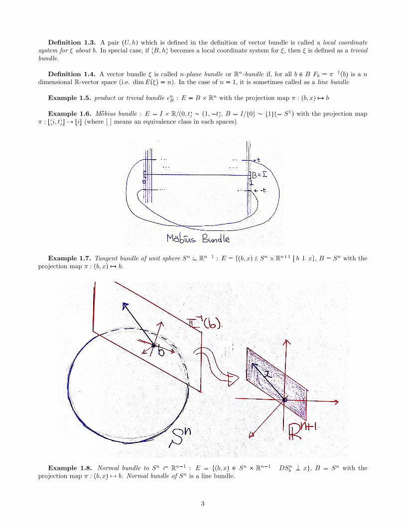
Example 1.6. M:obius bundle : E � I � R{p0, tq � p1,�tq, B � I{t0u � t1up� S1q with the projection mapπ : rpi, tqs ÞÑ ris (where [ ] means an equivalence class in each spaces)

Example 1.7. Tangent bundle of unit sphere Sn � Rn�1 : E � tpb, xq P Sn �Rn�1 | b K xu, B � Sn with theprojection map π : pb, xq ÞÑ b.

Example 1.8. Normal bundle to Sn � Rn�1 : E � tpb, xq P Sn � Rn�1 | DSnb K xu, B � Sn with theprojection map π : pb, xq ÞÑ b. Normal bundle of Sn is a line bundle.

3

Definition 1.9. The vector space ξ is called a smooth vector bundle if all objects and morphisms are containedin the category of smooth manifolds. To be specific, E,B are smooth manifolds, π is a smooth map, and h shouldbe diffeomorphism.

Example 1.10. Tangent bundle τM of a smooth manifold M : E � DM � tpx, vq P M � RA | v P DMxu,B � M with the projection map π : px, vq ÞÑ x. One might guess that τM � DM , but since DM has a structureof manifold and τM has a structure of vector bundle, it will be better to distinguish them.

After defining the vector bundle, we need to decide what vector bundles are the same. Since an equivalencerelation gives the classification scheme, the definition of isomorphism should be constructed at first.

Definition 1.11. Suppose that two vector bundles ξ and η are defined over the same base space B. ξ isisomorphic to η, if there exists a homeomorphism f : Epξq Ñ Epηq between the total spaces which maps eachvector space structured fibers Fbpξq isomorphically onto the corresponding vector space structured fibers Fbpηq. Inthis case, it is denoted by ξ � η.

To be more precise, an isomorphism f : Epξq Ñ Epηq is actually consisted of two maps, one is a homeomorphismf between two topological spaces Epξq and Epηq and the other is an isomorphic linear map Lf,b : Fbpξq Ñ Fbpηqwhich varies over the base point b P B � Bpξq � Bpηq. Moreover, in this case, f acts as an identity map on thebase space B. With all these description, f maps pb, xq where x P Fbpξq to pb, Lf,bpxqq where Lf,bpxq P Fbpηq.

Usually, category lovers defines morphisms before defining isomorphism. So, the order of definition mightconfuse some people who have read this. However, since we are focusing on classification rather than constructingspecific structures, morphism of this category which is named by bundle map, will be appeared later and in thatcase f |Bpξq could not be the identity map.

From now I will suggest the main words of this survey, parallelizable and the real projective space RPn.

Definition 1.11.(Parallelizable) A manifold M is called parallelizable if its tangent bundle τM is isomorphicto a trivial bundle.

In Boothby’s book, this terminology is defined by using the existence of linearly independent n-vector fields,which is the special case of cross-section, where n is the dimension of M . Although both use different words, bothindicates the same definition and since the concept of vector bundle is more general I will use this definition, andthe idea of Boothby will be appeared later in Theorem 1.17.

Definition 1.12. A cross-section of a vector bundle ξ with base space B is a continuous function s : B Ñ Epξqsuch that spbq P Fbpξq for all b P B. If M is a smooth manifold and ξ � τM , cross-section is usually called a vectorfield on M . Moreover, a cross-section called nowhere zero if spbq � 0 P Fbpξq for all b P B.

The word section comes from π � s � idB . Since the word section is defined as right inverse, the map s can beinterpreted as the right inverse of π. And if the reader is friendly with algebraic geometry, then one could guessthat the definition of cross-section is similar to the definition of section s : U Ñ

²PPU OX,P .

4

Remark 1.13. S2 is not parallelizable manifold. This can be proved by using the degree of a map f : S2 Ñ S2.(See [Hatcher,Algebraic Topology 135pg])

Although I will not suggest the proof of the following statement, but it is well known that S1, S3, S7 are theonly spheres that are paralellizable. This facts can be found in [Hatcher,Vector Bundles and K-theory 59pg].

Definition 1.14.(RPn and γ1n) The real projective space RPn can be defined as the quotient space of Sn � Rn�1,quotient by antipodal points. All points in RPn can be interpreted as t�xu where x P Sn. Moreover, the canonicalline bundle γ1n over RPn as following :

Epγ1nq � tpt�xu, vq P RPn � Rn�1 | Dc P R v � cxuπ : Epγ1nq Ñ RPn is defined by πpt�xu, vq � t�xu

Theorem 1.15. The bundle γ1n is not isomorphic to trivial bundle for n ¥ 1.

Proof. We can always define nowhere zero cross-section on a trivial real line bundle. However, if we define cross-section s : RPn Ñ Epγ1nq and quotient map p : Sn Ñ RPn, then there is a continuous real valued function on Sn

such that spppxqq � pt�xu, tpxqxq for all x P Sn. Since ppxq � pp�xq � t�xu, we can say that tp�xq � �tpxq.And by using the Intermediate Value Theorem, t should have a zero value in somewhere. Thus, we cannot definenowhere zero cross-section on RPn and this ends the proof.

The big game of the above theorem was proving the given bundle is non isomorphic, and key idea was thatthe trivial bundle admits a nowhere zero cross-section. Nowhere zero could be meaningful in line bundles, butthis concept will not be useful for higher dimension. Therefore, we need to find replacement for this idea and theconcept of linearly independent will help to generalize this concept.

Definition 1.16. A collection ts1, � � � , snu of cross-sections of a vector bundle ξ is called nowhere dependentif, for every b P B, the vectors s1pbq, � � � , snpbq are linearly independent in Fbpξq.

Nowhere dependent is also can be interpreted as everywhere linearly independent. And Now I will show thetheorem, which tells how can we generalize the idea of Theorem 1.15.

Theorem 1.17. An Rn-bundle ξ is trivial iff ξ possesses n cross-sections s1, � � � , sn which are nowhere depen-dent.

Key for this theorem is the following lemma.

Lemma 1.18. There are two vector bundles ξ and η which share the same base space B. Let f : Epξq Ñ Epηqis a continuous map such that f |B� idB and Lf,b : Fbpξq Ñ Fbpηq is a vector space isomorphism for all b P B.Then, f is a homeomorphism, thus isomorphism between two vector bundles.

5

This lemma is quite straightforward, because the proof only uses the local triviality of vector bundles andthe fact that invertible linear map is homeomorphism. And if we construct f : B � Rn Ñ Epξq such thatfpb, xq � x1s1pbq � � � � � xnsnpbq where x � px1, � � � , xnq then this lead us to prove the Theorem 1.17 by usingabove lemma.

Surprisingly, this theorem can be more refined in specific vector bundles, Euclidean Vector Bundles.

Definition 1.19. A Euclidean vector bundle is a real vector bundle ξ with a continuous function µ : Epξq Ñ Rsuch that for each b P B, µ |Fbpξq is a positive definite quadratic function. The µ is called as a Euclidean metric on ξ.

One might be curious why such a positive definite quadratic function is called metric. This is because, anyquadratic function implies a symmetric bilinear map, and positive definite allows this map to agree with the propertyof inner products. And by defining this map as inner product, this allows us to define norm and orthogonality andthis is why such quadratic form is called metric. In special case, if B � M is a smooth manifold and ξ � τM , aEuclidean metric µ : DM Ñ R is called Riemannian metric, and pM,µq is called Riemannian manifold.

So if I use this metric with the idea of Gram-Schmidt process, the Theorem 1.17 can be refined as following.

Theorem 1.20. ξ � εnB iff there exist n cross-sections s1, � � � , sn which ts1pbq, � � � , snpbqu forms an orthonormalbasis of Fbpξq for all b P B. (Specifically, Boothby called these cross-sections as coordinate frames for the case ofB �M is a smooth manifold and ξ � τM .)

If we can find any collection of nowhere dependent n cross-sections, we can show that given bundle is trivial.So these theorems(1.17 and 1.20) are very powerful to prove whether the given bundle is trivial when specific collec-tion of cross-sections is suggested. However, as we have shown in γ1n, some manifolds do not admit this condition.Moreover, for arbitrary vector bundle, it will be hard to find a full collection of nowhere dependent cross-sections.Therefore, some mathematicians tried to focus on deciding non-trivial vector bundles and this is the one reasonwhy the idea of Characteristic class pop up.

1.A. Basic ways to construct vector bundles

Before getting into the chapter of Stiefel-Whitney class, I will suggest several ways to construct vector bundles.Although I suggest examples of canonical line bundle γ1n and tangent bundle τM , there are a number of vectorbundles and usually they can be constructed by using a number of operators in vector spaces. To be specific, sincetensor product, Hom-functor, and direct sum preserves its vector space structure, these operators are often used toconstruct new bundles from given ones. Moreover, these tools will be useful, because new bundles can be studiedby using algebraic properties of these operators.

A.1. Restriction Let ξ be a vector bundle with projection π : E Ñ B and U be a subset of B. By takingE1 � π�1pUq, π |U : E1 Ñ U , we can get a new vector bundle ξ |U , namely the restriction of ξ to U .

A.2. Pull-Back or Induced Bundle Given a bundle ξ, an arbitrary topological space B1, and a mapf : B1 Ñ B, one can construct the induced bundle f�ξ over B1 as following :

Total space E1 � tpb, eq P B1 � E | fpbq � πpequThe projection map π1 : E1 Ñ B1 is defined by π1pb, eq � b

For a local coordinate system pU, hq for ξ, and U1 � f�1pUq,a local coordinate system pU1, h1q of f�ξ is defined by

h1 : U1 � Rn Ñ π�11 pU1q such that h1pb, xq � pb, hpfpbq, xqq.

One big property of pull-back is that it preserves smoothness. And moreover, if one makes induced bundlewith a bundle map, then induced bundle becomes isomorphic to original one.

6

Definition. Let η and ξ be vector bundles(they could have different base spaces). A continuous functiong : Epηq Ñ Epξq is called a bundle map if Lg,b : Fbpηq Ñ Fgpbqpξq is a vector space isomorphism for all b P Bpηq.

Lemma. If g : Epηq Ñ Epξq is a bundle map, then η � pg |Bpηqq�ξ.

A.3. Cartesian products Suppose that there are two vector bundles ξ1 and ξ2. The Cartesian product ξ1�ξ2is defined by making Cartesian products for all components.

Total space Epξ1 � ξ2q � E1 � E2, Base space Bpξ1 � ξ2q � B1 �B2,Projection map π1 � π2 : E1 � E2 Ñ B1 �B2, Fiber pπ1 � π2q

�1pb1, b2q � Fb1pξ1q � Fb2pξ2q.

A.4. Whitney Sums or Direct Sums Let ξ1, ξ2 be vector bundles over the same base space B. Letd : B Ñ B �B be a diagonal embedding such that b ÞÑ pb, bq. Then the bundle d�pξ1 � ξ2q over B is the Whitneysum of ξ1 and ξ2, and denoted by ξ1` ξ2. In this bundle, each fiber is isomorphic to the direct sum of original ones(i.e. Fbpξ1 ` ξ2q � Fbpξ1q ` Fbpξ2q).

Definition. A vector bundle ξ is called a sub-bundle of η if these two bundles have the same base space B,Fbpξq is a sub-vector space of Fbpηq for all b P B.

Lemma. Let ξ1 and ξ2 are sub-bundles of η with the property that Fbpηq � Fbpξ1q`Fbpξ2q for all b P B. Thenthis implies that η � ξ1 ` ξ2.

A.5. Orthgonal complements This method is only available for Euclidean vector bundles. Suppose that ηis an Euclidean vector bundle and ξ is sub-bundle of η. By taking all orthogonal parts of ξ in η we can define theorthogonal complement of ξ in η as following :

Total space EpξKq � tpb, xq P Epηq | b P B, x P Fbpηq, x K FbpξquThe projection map is the same as the projection map of η.

In this case, just because of Gram-Schmidt process, η � ξ ` ξK.

A.6. Using other continuous algebraic operations Key property of vector bundle is that all fiber hasthe vector space structure. And a person who have learned algebra might guess that there are a number of

7

operations that make new vector spaces. For example, for any real vector spaces V and W , HompV,W q, V bW ,V � � HompV,Rq, and ΛkV forms new vector spaces. Since all these operations are continuous, it is possible toapply these ideas to vector bundles and this lead us to make a number of new vector bundles.

2. Stiefel-Whitney Classes

Before saying about Stiefel-Whitney Classes, I like to talk about some background of cohomology first. Coho-mology can be simply defined as the dual of homology. The idea of homology is quite intuitive and stratightforward,but it is really hard to construct the intuitive view for cohomology. Although cohomology is hard to think intu-itively, a lot of mathematicians tried to research this because cohomology allowed them to get a number of invariantsof topological spaces. And the Stiefel-Whitney class is just one case of them.

Stiefel-Whitney class is a cohomology class of a vector bundle defined by four axioms. The existence anduniqueness will not be proved in this survey, but since there exists a proof, we will assume these two things in thissurvey. And basically HipB;Gq is defined by i-th singular cohomology group of B with coefficients in G, and Gwill always be Z{2Z for the Stiefel-Whitney classes.

Axiom 1. For any vector bundle ξ, there is a corresponding sequence of cohomology classes twipξqu wherewipξq P H

ipBpξq;Z{2Zq for all i � 0, 1, � � � . This class twipξqu is called the Stiefel-Whitney classes of ξ. Moreover,w0pξq � 1 which is the unit element in H0pBpξq;Z{2Zq, and wipξq � 0 for all i ¡ dimEpξq.

Axiom 2.(Naturality) If f : Bpξq Ñ Bpηq is a bundle map, then wipξq � f�wipηq.Axiom 3.(Whitney Product Theorem) Let ξ and η be vector bundles over the same base.

wkpξ ` ηq �k°

i�0

wipξq ` wk�ipηq, where ` is a cup product.

Usually, cup product will be omitted.Axiom 4. w1pγ

11q � 0, where γ11 is the canonical line bundle over RP 1.

With all these axioms, following propositions explain basic properties of Stiefel-Whitney classes.

Proposition 2.1. ξ � η ùñ wipξq � wipηq for all i

Proposition 2.2. ε is a trivial vector bundle ùñ wipεq � 0 for all i ¡ 0 (Usually, ε means trivial bundle)

Proposition 2.3. wipε` ηq � wipηq

Proposition 2.4. If ξ is an Euclidean Rn-bundle, and if admits nowhere linearly dependent k cross-sections,then

wn�k�1pξq � wn�k�2pξq � � � � � wnpξq � 0 (7 ξ � εkB ` pεkBqK)

Stiefel-Whitney classes are defined as the form of twipξqu. However, this sequence form makes people hardto look for its properties. By using the graded ring structure, there is a nice way to show Stiefel-Whitney classwithout losing any information.

Definition 2.5. H±

pB;Z{2Zq is the graded ring consisting of all formal infinite series a � a0 � a1 � a2 � � � �such that ai P H

ipB;Z{2Zq. The product of two elements in this graded ring is

pa0 � a1 � a2 � � � � qpb0 � b1 � b2 � � � � q � pa0b0q � pa1b0 � a0b1q � pa2b0 � a1b1 � a0b2q � � � �

The total Stiefel-Whitney class of Rn-bundle ξ over B is defined by

wpξq � 1� w1pξq � w2pξq � � � � � wnpξq � 0� � � � P H±

pB;Z{2Zq.

With the structure of the graded ring, we can briefly explain that wpξ ` ηq � wpξqwpηq.

8

Lemma 2.6. The collection of all infinite series

w � 1� w1 � w2 � � � � P H±

pB;Z{2Zq

with leading term 1 forms a field. In this case, the inverse is written by

w � 1� w1 � w2 � � � �

(7 Consider that all elements in power series with a unit leading term is a unit)

Lemma 2.7.(Whitney Duality Theorem) Let τM be the tangent bundle of a manifold M in Euclideanspace. If ν is the normal bundle, then

wipνq � wipτM q

This result immediately comes from the fact τM ` ν � ε and wpτM ` νq � wpτM qwpνq.

So far, I just suggested simple properties of Stiefel-Whitney classes. From now, I will try to reach to thegoal and show what real projective spaces are non-parallelizable with some lemmas. And we will pretend all realprojective spaces as Riemannian manifolds.

Lemma 2.8. H±

pRPn;Z{2Zq �pZ{2Zqrasxan�1y

More precise proof of this lemma is written in [Hilton and Wylie 151pg]. But the basic idea for this proof isthat RPn � e0 \ e1 \ � � � \ en where eis are i dimensional cell.

Lemma 2.9. wpγ1nq � 1� a

Proof. The standard inclusion j : RP 1 Ñ RPn implies a bundle map from γ11 to γ1n. By Axiom 2, j�wpγ1nq � wpγ11q.Because of Axiom 1 and 4 with Lemma 2.8, we can decide that wpγ11q � 1� a. Thus, all these information inducethe result.

With this lemma and the Whitney Duality Theorem, if we define γK as the orthogonal complement of γ1n inεn�1, we can easily show that

wpγKq � 1� a� � � � � an

Lemma 2.10. Define τ as the tangent bundle of smooth Riemannian manifold RPn. Then, the bundle τ isisomorphic to a bundle Hom(γ1n, γ

K).

Proof. Let L be a line through the origin in Rn�1 with L X Sn � tx,�xu. Also define LK � Rn�1 as theorthogonal complement of L in Rn�1. First of all, an elemnt in the tangent manifold DRPn can be defined bytpx, vq, p�x,�vqu where px, vq P DSn. Since x � x � 1 and x � v � 0, we can say that the set tpx, vq, p�x,�vqucorresponds to a linear mapping l : LÑ LK such that lpxq � v. With this idea, we can construct canonical vectorspace isomorphism from the fiber Ft�xupτq to the vector space Hom(L,LK) for each t�xu P RPn. This allows us

to decide τ � Hompγ1n, γKq.

Theorem 2.11. Let τ be a tangent bundle of RPn and ε1 be a trivial line bundle over the same base. Then,

τ ` ε1 � γ1n ` γ1n ` � � � ` γ1nloooooooooomoooooooooonpn�1q�times

Therefore, the total Stiefel-Whitney class of the tangent bundle of RPn is written by

wpτq � p1� aqn�1 � 1��n�11

�a�

�n�12

�a2 � � � � �

�n�1n

�an P HipRPn;Z{2Zq �

pZ{2Zqrasxan�1y

(wpτq is denoted by wpRPnq, and called as the total Stiefel-Whitney class of RPn)

9

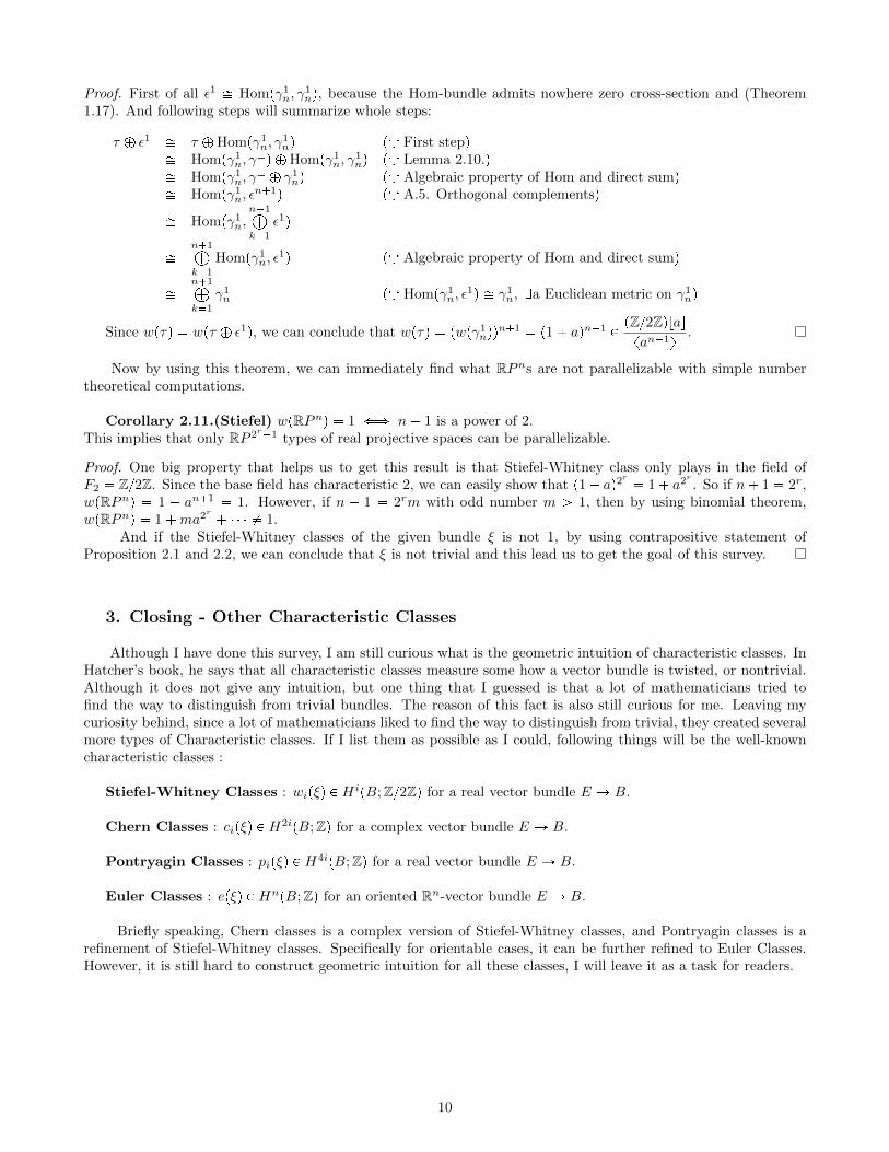
Proof. First of all ε1 � Hompγ1n, γ1nq, because the Hom-bundle admits nowhere zero cross-section and (Theorem

1.17). And following steps will summarize whole steps:

τ ` ε1 � τ `Hompγ1n, γ1nq p7 First stepq

� Hompγ1n, γKq `Hompγ1n, γ

1nq p7 Lemma 2.10.q

� Hompγ1n, γK ` γ1nq p7 Algebraic property of Hom and direct sumq

� Hompγ1n, εn�1q p7 A.5. Orthogonal complementsq

� Hompγ1n,n�1À

k�1

ε1q

�n�1À

k�1

Hompγ1n, ε1q p7 Algebraic property of Hom and direct sumq

�n�1À

k�1

γ1n p7 Hompγ1n, ε1q � γ1n, Da Euclidean metric on γ1nq

Since wpτq � wpτ ` ε1q, we can conclude that wpτq � pwpγ1nqqn�1 � p1� aqn�1 P

pZ{2Zqrasxan�1y

.

Now by using this theorem, we can immediately find what RPns are not parallelizable with simple numbertheoretical computations.

Corollary 2.11.(Stiefel) wpRPnq � 1 ðñ n� 1 is a power of 2.This implies that only RP 2r�1 types of real projective spaces can be parallelizable.

Proof. One big property that helps us to get this result is that Stiefel-Whitney class only plays in the field ofF2 � Z{2Z. Since the base field has characteristic 2, we can easily show that p1� aq2

r

� 1� a2r

. So if n� 1 � 2r,wpRPnq � 1 � an�1 � 1. However, if n � 1 � 2rm with odd number m ¡ 1, then by using binomial theorem,wpRPnq � 1�ma2

r

� � � � � 1.And if the Stiefel-Whitney classes of the given bundle ξ is not 1, by using contrapositive statement of

Proposition 2.1 and 2.2, we can conclude that ξ is not trivial and this lead us to get the goal of this survey.

3. Closing - Other Characteristic Classes

Although I have done this survey, I am still curious what is the geometric intuition of characteristic classes. InHatcher’s book, he says that all characteristic classes measure some how a vector bundle is twisted, or nontrivial.Although it does not give any intuition, but one thing that I guessed is that a lot of mathematicians tried tofind the way to distinguish from trivial bundles. The reason of this fact is also still curious for me. Leaving mycuriosity behind, since a lot of mathematicians liked to find the way to distinguish from trivial, they created severalmore types of Characteristic classes. If I list them as possible as I could, following things will be the well-knowncharacteristic classes :

Stiefel-Whitney Classes : wipξq P HipB;Z{2Zq for a real vector bundle E Ñ B.

Chern Classes : cipξq P H2ipB;Zq for a complex vector bundle E Ñ B.

Pontryagin Classes : pipξq P H4ipB;Zq for a real vector bundle E Ñ B.

Euler Classes : epξq P HnpB;Zq for an oriented Rn-vector bundle E Ñ B.

Briefly speaking, Chern classes is a complex version of Stiefel-Whitney classes, and Pontryagin classes is arefinement of Stiefel-Whitney classes. Specifically for orientable cases, it can be further refined to Euler Classes.However, it is still hard to construct geometric intuition for all these classes, I will leave it as a task for readers.

10

References

[1] John W.Milnor, James D.Stasheff, Characteristic Classes. Princeton University Press, (1974)

[2] Allen Hatcher, Vector Bundles and K-Theory. http://www.math.cornell.edu/ hatcher/VBKT/VB.pdf, (2009)

[3] Allen Hatcher, Algebraic Topology. http://www.math.cornell.edu/ hatcher/AT/AT.pdf, (2001)

[4] William M. Boothby, An Introduction to Differentiable Manifolds and Riemannian Geometry, Revised SecondEdition. Academic Press, (2010)

[5] P.J.Hilton, S.Wylie Homology Theory : An Introduction to Algebraic Topology. Cambridge University Press,(1960)

11