Non-prismatic Beams: a Simple and Effective Timoshenko-like Model

Giuseppe Balduzzia,∗, Mehdi Aminbaghaib, Elio Saccoc, Josef Füsslb, Josef Eberhardsteinerb, FerdinandoAuricchioa

aDepartment of Civil Engineering and Architeture (DICAr), University of Pavia, Pavia, ItalybInstitute for Mechanics of Materials and Structures (IMWS), Vienna University of Technology, Vienna, Austria

cDepartment of Civil and Mechanical Engineering, University of Cassino and Southern Lazio, Cassino, Italy

Abstract

The present paper discusses simple compatibility, equilibrium, and constitutive equations for a non-prismaticplanar beam. Specifically, the proposed model is based on standard Timoshenko kinematics (i.e., planarcross-section remain planar in consequence of a deformation, but can rotate with respect to the beam center-line). An initial discussion of a 2D elastic problem highlights that the boundary equilibrium deeply influencesthe cross-section stress distribution and all unknown fields are represented with respect to global Cartesiancoordinates. A simple beam model (i.e. a set of Ordinary Differential Equations (ODEs)) is derived,describing accurately the effects of non-prismatic geometry on the beam behavior and motivating equation’sterms with both physical and mathematical arguments. Finally, several analytical and numerical solutionsare compared with results existing in literature. The main conclusions can be summarized as follows. (i)The stress distribution within the cross-section is not trivial as in prismatic beams, in particular the shearstress distribution depends on all generalized stresses and on the beam geometry. (ii) The derivation ofsimplified constitutive relations highlights a strong dependence of each generalized deformation on all thegeneralized stresses. (iii) Axial and shear-bending problems are strictly coupled. (iv) The beam model isnaturally expressed as an explicit system of six first order ODEs. (v) The ODEs solution can be obtainedthrough the iterative integration of the right hand side term of each equation. (vi) The proposed simplemodel predicts the real behavior of non-prismatic beams with a good accuracy, reasonable for the most ofpractical applications.

Keywords: Non-prismatic Timoshenko beam, beam modeling, analytical solution, tapered beam, arches

1. Introduction

Non-prismatic beams –sometime mentioned also as beams with non-constant cross-section or beams of

variable cross-section– are a particular class of slender bodies, object of the practitioners interest due to thepossibility of optimizing their geometry with respect to specific needs (Timoshenko and Young, 1965; Au-ricchio et al., 2015). Despite the advantages that engineers can obtain from their use, non-trivial difficultiesoccurring in the non-prismatic beam modeling often lead to inaccurate predictions that vanish the gain ofthe optimization process (Hodges et al., 2010). As a consequence, an effective non-prismatic beam modelingstill represents a branch of the structural mechanics where significant improvements are required.

Within the large class of non-prismatic beams it is possible to recognize several families of beams char-acterized by peculiar properties and intrinsic modeling problems. Unfortunately, the literature lexicon isnot thorough and the language ambiguities could lead to some annoying misunderstanding. Therefore, in

∗Corresponding author. Adress: Dipartimento di Ingengeria Civile e Architettura (DICAr), Università degli Studi di Pavia,via Ferrata 3, 27100 Pavia Italy Email adress: giuseppe.balduzzi@unipv.it Phone: 0039 0382 985 468

Email addresses: giuseppe.balduzzi@unipv.it (Giuseppe Balduzzi), mehdi.aminbaghai@tuwien.ac.at (MehdiAminbaghai), sacco@unicas.it (Elio Sacco), Josef.Fuessl@tuwien.ac.at (Josef Füssl),josef.eberhardsteiner@tuwien.ac.at (Josef Eberhardsteiner), ferdinando.auricchio@unipv.it (Ferdinando Auricchio)

Preprint submitted to Elsevier April 29, 2016

order to discuss the existing approaches, we introduce some terminology that we are going to use in thisdocument.

• A prismatic beam is a prismatic slender body with straight center-line and constant cross-section.

• A curved beam is a body with a curvilinear center-line and constant cross-section (orthogonal to thecenter-line).

• A beam of variable cross-section is a beam with straight center-line and non-constant cross-section;sometime authors refer to this kind of bodies with the expression “non-prismatic beams” (Shooshtariand Khajavi, 2010; Attarnejad et al., 2010; Beltempo et al., 2015).

• A tapered beam is a beam of variable cross-section with the additional property that the cross-sectionsize varies linearly with respect to the axis coordinate; sometime authors refer to this kind of bodieswith the expression “beam of variable cross-section” (Cicala, 1939; Romano, 1996; Franciosi and Mecca,1998; Sapountzakis and Panagos, 2008).

• A twisted beam is a beam of variable cross-section with the additional property that the cross-sectionrotation around the axis coordinate varies.

• A non-prismatic beam is the most general case we can consider, i.e. a beam with curvilinear center-lineand non-constant cross-section.

Classical reference books treat separately curved beams and beams of variable cross-section, but do notprovide any specific indications for the non-prismatic beams (Timoshenko, 1955; Timoshenko and Young,1965). This distinction is substantially confirmed also in more recent books (Bruhns, 2003; Gross et al.,2012) and papers. As an example, Hodges et al. (2008, 2010) propose a model for a tapered beam whereasRajagopal et al. (2012); Yu et al. (2002) focus on curvilinear beams.

Focusing on curvilinear beams, the classical approach describes the beam geometry through a curvilinearcoordinate that runs along the beam center-line (Capurso, 1971; Bruhns, 2003). As a consequence, the cross-sections are defined as the intersection between the beam body and the plane orthogonal to the center-lineat a fixed curvilinear coordinate. Furthermore, the resulting forces –ensuring the beam equilibrium– areexpressed as function of a local coordinate system with the axes tangential, normal, and binormal to thecenter-line, respectively. For planar beams, the so far introduced choices lead to express the equilibriumthrough a system of 3 ODEs that are coupled and use non-linear coefficients (Rajasekaran and Padmanabhan,1989; Arunakirinathar and Reddy, 1992, 1993; Yu et al., 2002; Rajagopal et al., 2012). The immediateconsequence of this approach is that analytical solutions are available only for simple geometries, typicallybeams with constant curvature. An alternative approach was proposed by Gimena et al. (2008a) that expressboth displacements and resulting forces in a global coordinate system. The main advantage of the proposedapproach is the simplicity of the resulting ODEs that could be solved with successive integrations.

Focusing on beams of variable cross-section, the literature presents a number of possible models that canbe classified as follows:

• simple models, based on suitable modifications of Euler-Bernoulli or Timoshenko beam model coeffi-cients (Banerjee and Williams, 1985, 1986; Friedman and Kosmatka, 1993; Sapountzakis and Panagos,2008; Shooshtari and Khajavi, 2010),

• enhanced models, that consider an accurate description of stress (Rubin, 1999; Aminbaghai and Binder,2006) and are often derived from variational principles (Hodges et al., 2008, 2010; Auricchio et al.,2015; Beltempo et al., 2015),

• models based on 2D or 3D Finite Elements (FE), that often appear as the only possible path, especiallywhen an accurate description of unknown fields is required (Kechter and M.Gutkowski, 1984; El-Mezaini et al., 1991; Balkaya, 2001).

2

It is well known since the half of the past century that the simple models are no-longer effective in predictingthe real behavior of non-prismatic beams (Boley, 1963; Hodges et al., 2010). On the other hand, 2DFE models lead to a high computational effort. As a consequence, the enhanced models seem the bestcompromise.

It is worth noting that non-prismatic beams are often treated as beams of variable cross-section. In fact,both researchers and practitioners neglect the effects of the non-straight center-line for modeling simplicity(Portland Cement Associations, 1958; Timoshenko and Young, 1965; El-Mezaini et al., 1991; Tena-Colunga,1996; Balkaya and Citipitioglu, 1997; Ozay and Topcu, 2000). To the author’s knowledge, the few attemptsof a complete modeling of non-prismatic beams are Balduzzi (2013); Auricchio et al. (2015); Beltempo (2013);Beltempo et al. (2015) that use mixed variational principles and the dimension reduction method to deriveplanar beam models and Gimena et al. (2008b) that proposes a model for 3D non-prismatic beams and aneffective numerical procedure for the resolution of the Ordinary Differential Equations (ODEs) governing thebeam model. Unfortunately, the dimension reduction leads to equations with an unclear physical meaningand a complexity which seems scarcely manageable. Conversely, the model proposed by Gimena et al.(2008b) presents some limitations that will be discussed in the following.

The present paper aims at discussing a simple and effective non-prismatic planar beam model. Thederivation procedure is based on a rigorous treatment of the 2D elastic problem and exploits the simpleTimoshenko kinematics (i.e., planar cross-section remain planar in consequence of a deformation, but canrotate with respect to the beam center-line). The simplicity of resulting ODEs allows to provide the analyticalsolution for tapered beams and helps the understanding of several aspects that influence the effectiveness ofthe non-prismatic beam modeling.

The outline of the paper is as follows. Section 2 introduces the 2D elastic problem we are going totackle, Section 3 illustrates how to derive the non-prismatic beam model equations, Section 4 focuses ontapered beams for which some analytical results are provided and compared with other approaches existingin literature, Section 5 provides few numerical examples that highlight critical aspects and advantages of theproposed approach, and Section 6 discusses the final remarks and delineates future research’s developments.

2. 2D problem formulation

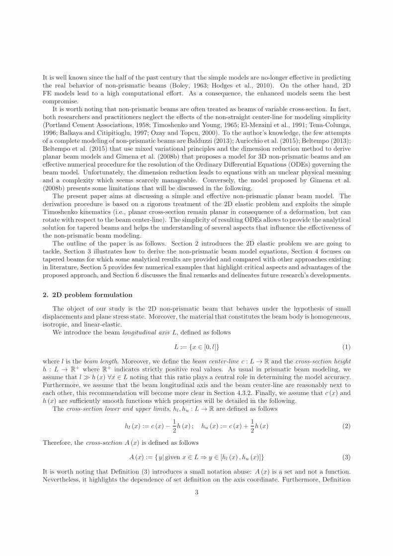
The object of our study is the 2D non-prismatic beam that behaves under the hypothesis of smalldisplacements and plane stress state. Moreover, the material that constitutes the beam body is homogeneous,isotropic, and linear-elastic.

We introduce the beam longitudinal axis L, defined as follows

L := x ∈ [0, l] (1)

where l is the beam length. Moreover, we define the beam center-line c : L → R and the cross-section height

h : L → R+ where R

+ indicates strictly positive real values. As usual in prismatic beam modeling, weassume that l ≫ h (x) ∀x ∈ L noting that this ratio plays a central role in determining the model accuracy.Furthermore, we assume that the beam longitudinal axis and the beam center-line are reasonably next toeach other, this recommendation will become more clear in Section 4.3.2. Finally, we assume that c (x) andh (x) are sufficiently smooth functions which properties will be detailed in the following.

The cross-section lower and upper limits, hl, hu : L → R are defined as follows

hl (x) := c (x)−1

2h (x) ; hu (x) := c (x) +

1

2h (x) (2)

Therefore, the cross-section A (x) is defined as follows

A (x) := y| given x ∈ L ⇒ y ∈ [hl (x) , hu (x)] (3)

It is worth noting that Definition (3) introduces a small notation abuse: A (x) is a set and not a function.Nevertheless, it highlights the dependence of set definition on the axis coordinate. Furthermore, Definition

3

(3) leads to cross-sections A (x) that are orthogonal to the longitudinal axis and not to the beam center-line,according to the approach proposed by Gimena et al. (2008a).

Using all the so far introduced notations, the 2D problem domain Ω results defined as follows

Ω := (x, y)| ∀x ∈ L → y ∈ A (x) (4)

Figure 1 represents the 2D domain Ω, the adopted Cartesian coordinate system Oxy, the lower and upperlimits y = hl (x) and y = hu (x), the center-line y = c (x), the longitudinal axis L, the initial, and the final

cross-sections A (0) and A (l).

o

y

h (x)

A (0)A (l)

hu (x)

hl (x)

x

l

p (x)

q (x)

m (x)

m (x)

c (x)L

Figure 1: Beam geometry, problem domain, coordinate system, dimensions, resulting loads, and adopted notations.

We denote the domain boundary as ∂Ω, such that ∂Ω := A (0) ∪ A (l) ∪ hl (x) ∪ hu (x). Moreover, weintroduce the partition ∂Ωs; ∂Ωt, where ∂Ωs and ∂Ωt are the displacement constrained and the loadedboundaries, respectively.

As usual in beam modeling, we assume that the lower and upper limits belong to the loaded boundary(i.e., hl (x) and hu (x) ∈ ∂Ωt) whereas al least one of the initial and final cross-sections A (0) and A (l)belong to the displacement constrained boundary ∂Ωs that can not be an empty set in order to ensuresolution uniqueness. The boundary load distribution ttt : ∂Ωt → R

2 is assumed to vanish on lower and upperlimits (i.e., ttt|hl,u

= 000). It is worth noting that this hypothesis is not strictly necessary to the beam modelderivation and therefore it can be removed with suitable modifications of the model equations. Finally, adistributed load fff : Ω → R

2 is applied to the beam body and a suitable boundary displacement functionsss : ∂Ωs → R

2 is assigned in order to opportunely reproduce the constraint usually adopted in structuralmechanics.

We highlight that the proposed geometry formulation is as general as possible and recovers easily boththe cases of curved beam and beam of variable cross-section, assuming respectively that h (x) or c (x)are constant. Furthermore, with respect to the classical definition of curved beams (Capurso, 1971), theproposed approach does not require conditions on center-line’s second derivative. Conversely, the proposedapproach can tackle only center-lines and thickness with bounded first derivatives, for reasons that will bemore clear in the following. This could be a limit since –as an example– the proposed method does not havethe capability to describe a semi-circular beam. Nevertheless, the so far highlighted limitation can be easilybypassed through the use of approximations or simple tricks.

We introduce the stress field σσσ : Ω → R2×2s , the strain field εεε : Ω → R

2×2s , and the displacement vector

field sss : Ω → R2, where R

2×2s denotes the space of symmetric, second order tensors. Thereby, the 2D elastic

4

problem corresponds to the following boundary value problem

εεε = ∇ssss in Ω (5a)

σσσ =DDD : εεε in Ω (5b)

∇ ·σσσ + fff = 000 in Ω (5c)

σσσ ·nnn = ttt on ∂Ωt (5d)

sss = sss on ∂Ωs (5e)

where ∇s ( · ) is the operator that provides the symmetric part of the gradient, ∇ · ( · ) represents the diver-gence operator, ( · ) : ( · ) represents the double dot product, and DDD is the fourth order tensor that defines themechanical properties of the material. Equation (5a) is the 2D compatibility relation, Equation (5b) is the2D material constitutive relation, and Equation (5c) represents the 2D equilibrium relation. Equations (5d)and (5e) are respectively the boundary equilibrium and the boundary compatibility conditions, where nnn isthe outward unit vector, defined on the boundary.

O x

ynx

ny

nnn

1

hu(x)

h′

u(x)

Figure 2: Outward unit vector evaluated on the upper limit function h′

u (x).

As illustrated in Figure 2, the outward unit vectors on the lower and upper limits result as follows

nnn|hl(x) =

1√1 + (h′

l (x))2

h′

l (x)−1

; nnn|hu

(x) =1√

1 + (h′u (x))

2

−h′

u (x)1

(6)

where ( · )′ denotes the derivative with respect to the independent variable x. The boundary equilibrium(5d) on lower and upper limits (i.e., (σσσ ·nnn)|hl∪hu

= 000) could be expressed as follows

[σx ττ σy

]nx

ny

=

00

⇒

σxnx + τny = 0

τnx + σyny = 0(7)

where we omit the indication of the restriction ( · )|hl∪hufor notation simplicity. Manipulating Equation

(7), we express τ and σy as function of σx; using the outward unit vector nnn definition (6), we obtain thefollowing expressions for boundary equilibrium

τ = −nx

nyσx = h′σx (8a)

σy =n2x

n2y

σx = (h′)2σx (8b)

where h indicates either hl (x) or hu (x), accordingly to the point where we are evaluating the function.Equation (8) is defined only for non-vanishing ny, therefore we need to require that first derivatives of lowerand upper limits –and consequently of center-line and cross-section height– are bounded.

As already highlighted in (Auricchio et al., 2015), σx could be seen as the independent variable thatcompletely defines the stress state on the lower and upper surfaces. Moreover, as stated by Boley (1963)and Hodges et al. (2008, 2010) the lower and upper limit slopes h′

l and h′

u play a central role in boundaryequilibrium, determining the stress distribution within the cross-section A (x).

5

3. Simplified 1D model

This section aims at deriving the ODEs representing the beam model. In fact, the solution of the2D problem introduced in Section 2 is in general not available. As a consequence, in order to obtain anapproximated solution, practitioners consider simplified models properly called beam models. The non-prismatic beam model derivation consists of 4 main steps

1. derivation of compatibility equations,

2. derivation of equilibrium equations,

3. stress representation, and

4. derivation of simplified constitutive relations

that correspond to the subdivision of the present section.Figure 1 represents the domain of the beam model we are going to develop. It is worth noting that

Equation (5) considers a 2D region as problem domain, the classical curved beam models considers thecenter-line c (x), and the beam model we are going to develop considers the beam axis L. Furthermore, weremark that all the generalized variables we are going to use are referred to the global Cartesian coordinatesystem Oxy.

In Figure 1, q (x), m (x), and p (x) are the horizontal, bending, and vertical resulting loads defined as

q (x) =

∫

A(x)

fx (x, y) dy; m (x) = −

∫

A(x)

yfx (x, y) dy; p (x) =

∫

A(x)

fy (x, y) dy (9)

where fx (x, y) and fy (x, y) are the horizontal and vertical components of the load vector fff .

Finally, for convenience during the model derivation, we introduce the linear function b (y) defined as

b (y) =2 (c (x)− y)

h (x)(10)

We note that b (y) represents an odd function with respect to the cross-section A (x), it vanishes at y = c (x),and it is equal to ±1 at y = hu/l (x).

3.1. Compatibility equations

In order to develop the non-prismatic beam model, we assume that the kinematics usually adopted forprismatic Timoshenko beam models is still valid. Therefore, we represent 2D displacement field sss (x, y) interms of three 1D functions indicated as generalized displacements: the horizontal displacement u (x), therotation ϕ (x), and the vertical displacement v (x). Specifically, we assume that the beam body displacementsare approximated as follows:

sss (x, y) ≈

u (x)−

h (x)

2b (y)ϕ (x)

v (x)

(11)

We introduce the generalized deformations i.e., the horizontal deformation ε0 (x), the curvature χ (x),and the shear deformation γ (x) respectively defined as follows

ε0 (x) =1

h (x)

∫

A(x)

εxdy; χ (x) =12

h3 (x)

∫

A(x)

εx (c (x)− y) dy; γ (x) =1

h (x)

∫

A(x)

εxydy (12)

where εx and εxy are the components of the strain tensor εεε.Therefore, the beam compatibility is expressed through the following equations

ε0 (x) = u′ (x)− c′ (x)ϕ (x) (13a)

χ (x) = −ϕ′ (x) (13b)

γ (x) = v′ (x) + ϕ (x) (13c)

6

We note that, with respect to the prismatic beam compatibility, a new term c′ (x)ϕ (x) appears inEquation (13a). Its physical meaning is illustrated in Figure 3 that shows that, if the center-line is non-horizontal, a rotation induces non-negligible horizontal displacement. On the other hand, considering astraight center-line parallel to the beam axis, this term vanishes recovering the more familiar compatibilityequations usually adopted for prismatic beams.

1

c′(x)

θ

ϕ

dx

ϕdx

ϕdx sin (θ) ≈ ϕdxc′(x)

ϕdx cos (θ) ≈ ϕdx

Figure 3: Schematic representation of displacements induced by rotation.

3.2. Equilibrium equations

We introduce the generalized stresses i.e., the resulting horizontal stress H (x), the resulting bending

moment M (x), and the resulting vertical stress V (x) respectively defined as follows

H (x) =

∫

A(x)

σxdy (14a)

M (x) =

∫

A(x)

σx (c (x)− y) dy (14b)

V (x) =

∫

A(x)

τdy (14c)

We use the virtual work principle in order to obtain the beam equilibrium equations. The internalwork Lint can be calculated multiplying the virtual generalized deformations δε0 (x) , δχ (x), and δγ (x)(that satisfy Equation (13)) for the corresponding equilibrated generalized stresses H (x), M (x), and V (x).Analogously, the external work Lext can be calculated multiplying the virtual generalized displacementsδu (x), δϕ (x), and δv (x) for the corresponding resulting loads. Equalizing internal and external works weobtain

Lint =

∫

L

[δε0 (x) ·H (x) + δχ (x) ·M (x) + δγ (x) ·V (x)] dx =

Lext =

∫

L

[δu (x) · q (x)− δϕ (x) ·m (x) + δv (x) · p (x)] dx

(15)

Substituting compatibility equations (13) in Equation (15) we obtain:

∫

L

[[δu′ (x)− c′ (x) δϕ (x)] ·H (x)− δϕ′ (x) ·M (x) + [δv′ (x) + δϕ (x)] ·V (x)] dx =

∫

L

[δu (x) · q (x) − δϕ (x) ·m (x) + δv (x) · p (x)] dx

(16)

7

Integrating by parts the terms that apply derivatives to virtual generalized displacements and later collectinggeneralized displacements, we obtain

−

∫

L

δu (x) ·H ′ (x) dx+

∫

L

δϕ (x) · [M ′ − c′ (x)H (x) + V (x)] dx−

∫

L

δv (x) ·V ′ (x) dx =

∫

L

(δu (x) · q (x)− δϕ (x) ·m (x) + δv (x) · p (x)) dx

(17)

In order to satisfy Equation (17) for all possible virtual generalized displacements, generalized stresses mustsatisfy the following equations

H ′ (x) = −q (x) (18a)

M ′ (x) −H (x) · c′ (x) + V (x) = −m (x) (18b)

V ′ (x) = −p (x) (18c)

that therefore are the equilibrium relations.

H

MV

p(x) dx

q(x) dx

m(x) dx

dx

c(x) c′(x) dx

V + dV

H + dH

M + dM

Figure 4: Resulting loads and generalized stresses acting on a portion of non-prismatic beam of length dx.

It is worth noting that equilibrium equations (18) can be obtained considering the equilibrium of aportion of non-prismatic beam of length dx (see Figure 4). Furthermore, Equation (18b) is a generalizationof prismatic beam rotation equilibrium. Specifically, the term H (x) · c′ (x) takes into account the momentinduced by horizontal resulting forces that are applied at different y coordinate in each cross-sections. Asexpected, the coefficient c′ (x) vanishes for prismatic beams, leading to the well known prismatic beamequilibrium equation.

3.3. Recovery of cross-section stress distributions

The Timoshenko beam recovers the stress distributions within the cross-section through the followingassumptions:

• the horizontal stress σx has a linear distribution,

• the vertical stress σy has a vanishing value,

• the shear stress τ has a parabolic distribution, according to Jourawski theory (Timoshenko, 1955,Chapter IV).

8

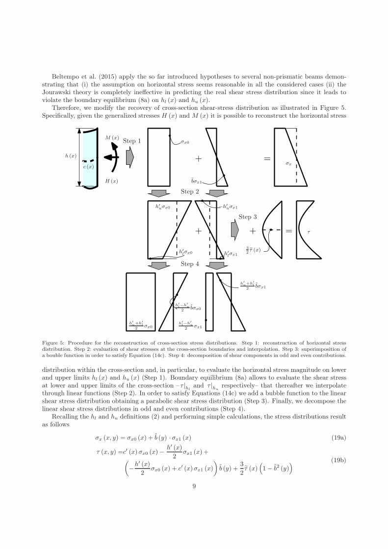
Beltempo et al. (2015) apply the so far introduced hypotheses to several non-prismatic beams demon-strating that (i) the assumption on horizontal stress seems reasonable in all the considered cases (ii) theJourawski theory is completely ineffective in predicting the real shear stress distribution since it leads toviolate the boundary equilibrium (8a) on hl (x) and hu (x).

Therefore, we modify the recovery of cross-section shear-stress distribution as illustrated in Figure 5.Specifically, given the generalized stresses H (x) and M (x) it is possible to reconstruct the horizontal stress

+

+ + =

=

M (x)

H (x)

h (x)

c (x)

3

2τ (x)

σx0

bσx1

σx

τ

h′

uσx0

h′

lσx0

−h′

uσx1

h′

lσx1

h′

u+h′

l2

σx0h′

l−h′

u

2σx1

h′

l−h′

u

2bσx0

h′

u+h′

l2

bσx1

Step 1

Step 2

Step 3

Step 4

Figure 5: Procedure for the reconstruction of cross-section stress distributions. Step 1: reconstruction of horizontal stressdistribution. Step 2: evaluation of shear stresses at the cross-section boundaries and interpolation. Step 3: superimposition ofa bouble function in order to satisfy Equation (14c). Step 4: decomposition of shear components in odd and even contributions.

distribution within the cross-section and, in particular, to evaluate the horizontal stress magnitude on lowerand upper limits hl (x) and hu (x) (Step 1). Boundary equilibrium (8a) allows to evaluate the shear stressat lower and upper limits of the cross-section –τ |hl

and τ |hurespectively– that thereafter we interpolate

through linear functions (Step 2). In order to satisfy Equations (14c) we add a bubble function to the linearshear stress distribution obtaining a parabolic shear stress distribution (Step 3). Finally, we decompose thelinear shear stress distributions in odd and even contributions (Step 4).

Recalling the hl and hu definitions (2) and performing simple calculations, the stress distributions resultas follows

σx (x, y) = σx0 (x) + b (y) ·σx1 (x) (19a)

τ (x, y) =c′ (x)σx0 (x)−h′ (x)

2σx1 (x) +

(−h′ (x)

2σx0 (x) + c′ (x)σx1 (x)

)b (y) +

3

2τ (x)

(1− b2 (y)

) (19b)

9

where the variables σx0 (x), σx1 (x), and τ (x) result defined as follows

σx0 (x) =H (x)

h (x); σx1 (x) = M (x)

6

h2 (x); τ (x) =

(−V (x)

h (x)− c′ (x) σx0 (x) +

h′ (x)

2σx1 (x)

)(20)

Finally, few algebraic steps allow us to express the shear stress distribution as illustrated in the following

τ (x, y) =

(c′ (x) σx0 (x) −

h′ (x)

2σx1 (x)

)(−1

2+

3

2b2 (y)

)

−

(h′ (x)

2σx0 (x)− c′ (x)σx1 (x)

)b (y) +

3

2τ0 (x)

(1− b2 (y)

) (21)

where the variable τ0 (x) results defined as follows

τ0 (x) = −V (x)

h (x)(22)

It is worth noting that the previously introduced quantities have a clear physical meaning:

• σx0 (x) is the mean value of the horizontal stress within the cross-section,

• σx1 (x) is the maximum horizontal stress value induced by bending moment that occurs at the cross-section lower limit, and

• τ0 (x) is the shear stress mean value.

In Equation (21), the shear distribution τ depends not only on V (x), but also on H (x) and M (x) thatdetermine not only the magnitude but also the shape of the shear distribution. Finally, Equation (21) leadsto conclude that the maximum shear stress does not occur in correspondence of the beam center-line, asnoted by Paglietti and Carta (2007, 2009).

The assumption of vanishing vertical stresses σy (x, y) = 0 agrees with the assumptions of prismaticbeam stress recovery, significantly simplifying the beam model equations, but leads to violate Equation(8b). Fortunately, this choice will not deeply worsen the model capability, as the numerical examples ofSection 5 will illustrate. On the other hand, readers may refer to (Auricchio et al., 2015; Beltempo et al.,2015) for more refined models that do not neglect the contribution of vertical stresses.

The recovery relation (21) is well known since the first half of the twentieth century. In particular,referring to the analytical solution of the 2D equilibrium equation (5c) for an infinite long wedge, Atkin(1938); Cicala (1939); Timoshenko and Goodier (1951) express the stress distribution as the combinationof some trigonometric functions. More in detail, Timoshenko and Goodier (1951) state that a parabolicshear distribution is an approximation reasonably accurate in the case of small boundary slope. Later on,Krahula (1975) extends the so far mentioned results to tapered beams, recovering equations substantiallyidentical to (19a) and (21). Furthermore, more recently, Bruhns (2003, Example 3.9) notes that (i) theshear distribution in a tapered beam has no longer a distribution similar to the prismatic beams, (ii) theshear distribution depends not only on resulting shear, but also in bending moment and resulting horizontalstress, and (iii) the maximum shear could occur everywhere in the cross-section.

However, it is worth noting that all the so far mentioned references consider the stress representation(19a) and (21) valid only for tapered beams whereas we are extending the representation’s validity to moregeneral cases. The numerical examples reported in (Auricchio et al., 2015; Beltempo et al., 2015) partiallyconfirm that the recovery relations (19a) and (21) remain valid also in more general situations. Obviously,the effectiveness of stress description as well as of the beam model will decrease increasing the boundaryslope and decreasing the beam slenderness, as it happens for tapered beams.

10

3.4. Simplified constitutive relations

To complete the Timoshenko-like beam model we need to introduce some simplified constitutive relationsthat define the generalized deformations as a function of generalized stresses.

The constitutive relation of the Timoshenko prismatic beam model needs a correction factor k that isintroduced in order to equalize the work of generalized shear stresses and deformations that considers onlytheir mean values and the work of real shear stresses and strains that takes into account the real stress andstrain distributions within the cross-section. In particular, for the simple case of a rectangular cross-section,the shear correction factor could be evaluated through the following formula

k =

∫A

1Gτ2dy

h (x) 1G

V 2(x)h2(x)

=1

h (x)

∫

A

9

4

(1− b2 (y)

)2dy =

5

6(23)

It is worth noting that Equation (23) is effective because only the magnitude varies while the shear distri-bution has the same shape in all the cross-sections. Unfortunately, this does not hold for the non-prismaticbeam. This simple consideration, together with the non trivial dependence τ (x, y) on H (x) and M (x) –seeEquation (21)– lead to conclude that the prismatic beam constitutive relations are not satisfactory for thenon-prismatic beams and a more refined approach must be adopted.

In particular, we consider the stress potential, defined as follows

Ψ∗ =1

2

(σ2x (x, y)

E+

τ2 (x, y)

G

)(24)

where E is the Young’s modulus and G is the shear modulus. Substituting the stress recovery relations(19a) and (21) in Equation (24), the generalized deformations result as the derivatives of the stress potentialwith respect to the corresponding generalized stress. Therefore we have

ε0 (x) =

∫

A(x)

∂Ψ∗

∂H (x)dy = εHH (x) + εMM (x) + εV V (x) (25a)

χ (x) =

∫

A(x)

∂Ψ∗

∂M (x)dy = χHH (x) + χMM (x) + χV V (x) (25b)

γ (x) =

∫

A(x)

∂Ψ∗

∂V (x)dy = γHH (x) + γMM (x) + γV V (x) (25c)

where

εH =

(c′2 (x)

5Gh (x)+

h′2 (x)

12Gh (x)+

1

Eh (x)

); εM = χH = −

8c′ (x)h′ (x)

5Gh2 (x); εV = γH =

c′ (x)

5Gh (x)

χM =

(9h′2 (x)

5Gh3 (x)+

12c′2 (x)

Gh3 (x)+

12

Eh3 (x)

); χV = γM = −

3h′ (x)

5Gh2 (x); γV =

6

5Gh (x)

It is worth noting the following statements.

• Unlike the prismatic beam models, the generalized deformations depend on all generalized stresses.

• It is possible to recognize in εH , χM , and γV the terms of prismatic beam constitutive laws

ε0 (x) =H (x)

Eh (x); χ (x) =

12M (x)

Eh3 (x); γ (x) = −

V (x)

kGh (x)(26)

• The shear correction factor, as well as the other coefficients, results naturally from the derivationprocedure, bypassing the problem of their evaluation.

11

To the author’s knowledge, Vu-Quoc and Léger (1992) are the former researchers mentioning the non-trivial dependence of all generalized deformations on all generalized stresses. Considering the shear bendingof a tapered beam, the authors derive the beam’s flexibility matrix using the principle of complementaryvirtual work. Later on, deriving a model for a tapered beam, Rubin (1999) and Aminbaghai and Binder(2006) consider the fact that the bending moment produces also shear deformation and the shear forceproduces a curvature. Unfortunately, they do not consider the effect of a non-horizontal center-line and Rubin(1999) use different coefficients with respect to the ones reported in Equations (25), resulting energeticallyinconsistent. Conversely, for the model derivation, Hodges et al. (2008); Auricchio et al. (2015); Beltempoet al. (2015) use variational principles that have the advantage to naturally derive the constitutive relations,but could lead to more complicated equations, as already highlighted in Section 1.

3.5. Remarks on beam model’s ODEs

In the following we resume the beam model’s ODEs according to the notation adopted by Gimena et al.(2008a).

H ′ (x)V ′ (x)M ′ (x)ϕ′ (x)v′ (x)u′ (x)

=

0 0 00 0 0 000

−c′ (x) 1 0χH χV χM 0 0 0γH γV γM 1 0 0εH εV εM −c′ (x) 0 0

H (x)V (x)M (x)ϕ (x)v (x)u (x)

−

q (x)p (x)m (x)000

(27)

With respect to Equation (27), it is worth noting what follows.

• The equations are naturally expressed as an explicit system of first order ODEs.

• Similar to Gimena et al. (2008a), the matrix that collects equations’ coefficients has a lower triangularform with vanishing diagonal terms. As a consequence, the analytical solution can easily be obtainedthrough an iterative process of integration done row by row, starting from H (x) and arriving at u (x).

• Reducing the beam model proposed by Gimena et al. (2008a) to a 2D case, it is easy to recog-nize the same structure in equilibrium and kinematics relations. Specifically Gimena et al. (2008a)use trigonometric coefficients whereas we use the corresponding linearized ones (i.e., we assume thatsin (θ) ≅ tan (θ) ≅ θ).

• The sub-matrix that collects the constitutive relation coefficients is symmetric with respect to theanti-diagonal.

• Finally, the sub-matrix that collects the constitutive relation coefficients is completely full whereasGimena et al. (2008a) neglect coupling between curvature, horizontal, and vertical resulting stresses(i.e., χH = χV = εM = γM = 0). Examples reported in Section 5 will illustrate that all the terms ofthe simplified constitutive relations plays a crucial role and are in general not negligible.

Now we move our attention back to the equilibrium (18) and the compatibility (13) equations. It isworth noting that the use of a global Cartesian coordinate system presents the following main advantages.

• Both the beam equilibrium and compatibility are not influenced by the cross-section size, which onthe contrary plays a central role in constitutive relations.

• Horizontal and vertical equilibrium are expressed through independent equations, whereas in classicalformulation (Bruhns, 2003, Chapter 5) tangential and normal equilibrium equations are coupled.

Furthermore, we note that few researchers follow the path of using a global Cartesian coordinate systemwith cross-sections orthogonal to x− axis. Fung and Kaplan (1952) investigate the buckling of beams withsmall curvatures and Borri et al. (1992); Popescu et al. (2000); Rajagopal and Hodges (2014) propose beam

12

models considering oblique cross-sections. On the other hand, Vogel (1993) develops a second order Euler-Bernoulli beam model for curved beams in large displacement regime and Gimena et al. (2008a,b) develop3D non-prismatic beam models expressing the resulting forces in a global coordinate system.

Finally, if we neglect shear deformation in the proposed model and the second order terms in (Vogel,1993) –i.e., if we lead both models to use the same assumptions– we obtain the same equations, showingonce more that the proposed model has the capability to recover simpler models available in literature.

4. Tapered beam analytical solution

This section discusses the analytical solution of the ODEs governing the problem (27) for the simple caseof a tapered beam. Specifically, we consider a beam with an inclined center-line, as illustrated in Figure 6.

O

x

y

l

h (0)

h (l)

h1 =h (l)− h (0)

l

1

c1

Figure 6: Tapered beam considered for the evaluation of the analytical solution: geometry and parameter’s definitions.

The center-line and the thickness have the following analytical expressions

c (x) = c1x; h (x) = h1x+ h0 (28)

4.1. Homogeneous solution

Considering the geometry so far introduced, the homogeneous solution of the beam model ODEs (27) is

H (x) =C6

M (x) = (c1C6 − C5)x+ C4

V (x) =C5

ϕ (x) =−3(20Ec21 + 3Eh2

1 + 20G)

10EGh21h

2 (x)(h0 (c1C6 − C5)− h1C4)

+c1(60Ec21 + Eh2

1 + 60G)

5EGh21h (x)

C6 −6(10Ec21 + Eh2

1 + 10G)

5EGh21h (x)

C5 + C3

u (x) =log (h (x))

60EGh31

(72c1

(10Ec21 − Eh2

1 + 10G)(c1C6 − C5) + 5h2

1 (Eh1 + 12G)C6 + 12c1Eh21C5

)

−c1(60Ec21 − 7Eh2

1 + 60G)

10EGh31h (x)

(h0 (C5 − c1C6) + h1C4)

+ c1xC3 + C2

v (x) =−log (h (x))

5EGh31

(c1(60Ec21 − Eh2

1 + 60G)C6 − 3

(20Ec21 + 3Eh2

1 + 20G)C5

)

−3(20Ec21 + Eh2

1 + 20G)

10EGh31h (x)

(c1h0C6 − h0C5 − h1C4)− xC3 + C1

(29)

13

where the parameters C1, C2, C3, C4, C5, and C6 depend on boundary conditions.The analytical solution of non-prismatic beam (29) uses rational and logarithmic terms whereas the ana-

lytical solution of prismatic beam uses polynomial terms. As a consequence, the polynomials usually adoptedin structural analysis in order to reconstruct the prismatic beam displacement given the nodal displacementsor as shape functions for FE software, are no longer effective for non-prismatic beams. Furthermore, thenon-prismatic beam stiffness matrix has a completely different structure that is influenced by the non-trivialdistribution of displacements along the beam longitudinal axis and the strong coupling of all equations. Thehomogeneous solution (29) can be used to overcome these problems, nonetheless these aspects lie outsidethis paper’s aims and will be object of a further scientific paper.

4.2. Particular solution

Considering a constant vertical load p (x) = p we obtain the following particular solution for the beammodel ODEs (27).

H (x) =0

M (x) =1

2px2

V (x) =− px

ϕ (x) =−3p

20EGh31

(2(20Ec21 + Eh2

1 + 20G)log (h (x))−

h20

(20Ec21 + 3Eh2

1 + 20G)

h2 (x)

+ 8h0

(10Ec21 + Eh2

1 + 10G)

h (x)

)

u (x) =−3c1p

10EGh41

((20Ec21 + Eh2

1 + 20G)h (x) (log (h (x))− 1) +

4

3

(60Ec21 − Eh2

1 + 60G)h0 log (h (x))

+(20Ec21 + Eh2

1 + 20G)h (x) +

h20

(60Ec21 − 7Eh2

1 + 60G)

6h (x)+ 2xEh3

1

)

v (x) =3p

EGh41

((20Ec21 + Eh2

1 + 20G)h (x) (log (h (x))− 1) + 4h0

(20Ec21 + 3Eh2

1 + 20G)log (h (x))

+1

2h (x)

(20Ec21 + Eh2

1 + 20G)h20 −

3xEh31

10

)

(30)

4.3. Asymptotic analysis

In this section, we perform some tests in order to evaluate robustness and correctness of the beam model.Specifically we are going to investigate two main aspects:

1. the behavior of the beam solution when the geometry tends to become prismatic,

2. the capability of the beam model to recover the solution of a tapered beam that has the straight axisrotated with respect to the principal Cartesian coordinate system.

We consider a tapered cantilever, clamped in the initial cross-section and loaded with a vertical con-centrated force in the final cross-section i.e., u (0) = ϕ (0) = v (0) = H (l) = M (l) = 0, and V (l) = 1N.Furthermore, we assume the following values:

l = 10mm; h (0) = αh (l) ; h (l) = 1mm; E = 105 MPa; G = 4 · 104 MPa (31)

where α is the ratio between the maximum and the minimum cross-section sizes.

14

4.3.1. Beam behavior for vanishing taper slope

To evaluate the non-prismatic beam behavior for vanishing taper slope, we consider two cases:

1. a cantilever with an horizontal center-line i.e., c (x) = 0 where all the cross-sections are symmetricwith respect to the beam longitudinal axis, denoted in the following as symm

2. a cantilever with an horizontal lower limit i.e., hl (x) = 0 and c (x) = (1− α) h (l) x2l , denoted in the

following as unsym

We investigate the model behavior when the parameter α → 1 i.e., when the beam becomes prismatic.Since it is not possible to evaluate analytically the displacement limit, we evaluate the maximum verticaldisplacement v (l) varying α between 2 and 1 + 1 · 10−9mm.

The maximum vertical displacement for the Timoshenko beam solution, indicated in the following as vasassume the following value:

vas =1

3

V (l) l3

E h3

12

+6

5

V (l) l

Gh= 0.0403mm (32)

Figure 7(a) plots the variation of the maximum displacement as a function of the parameter α whereas

10−10

10−8

10−6

10−4

10−2

100

0.01

0.015

0.02

0.025

0.03

0.035

0.04

(α − 1)

v(l)[m

m]

symmunsym

vas

(a) Maximum vertical displacement v (l) evaluated fordifferent geometries and values of α.

10−10

10−8

10−6

10−4

10−2

100

10−10

10−8

10−6

10−4

10−2

100

(α − 1)

eas

symmunsym

(b) Asymptotic error eas evaluated for differentgeometries and values of α.

Figure 7: Asymptotic behavior of a tapered cantilever loaded with a shear force V (l) = 1N applied in the final cross-section.

Figure 7(b) plots the asymptotic error defined as

eas =|v (l)− vas|

|vas|(33)

We note that the effect of the non-horizontal center-line is negligible. Furthermore, the parameter α hasa meaningful influence on the beam behavior for values greater than 1 + 1 · 10−3. Performing calculationswith standard double precision numbers, the solution starts to worsen for α < 1 + 1 · 10−4 and calculationsdo not run for a < 1 + 1 · 10−7. Therefore, we use 50 digits precision numbers for the evaluation of theresults reported in Figure 7.

Concluding, the model converges to the Timoshenko solution as expected. Furthermore, the analysishighlights some numerical problems in the model solution that fortunately occur for geometries withoutpractical interest.

4.3.2. Effects of beam rotation

This subsection discusses the effect of a rotation of the global Cartesian coordinate system with respectto which we express the beam geometry. Due to the rotation θ of the Cartesian coordinate system, thecross-sections will not remain perpendicular to the beam center-line and the beam geometry will change as

15

O

x1

y1

x

y

θ

P

h(0)h (l)

l

Figure 8: Symmetric tapered cantilever, geometry defintion through different Cartesian coordinate systems l = 10mm, h (0) =αh (l), h (l) = 1mm, P = 1N, E = 105 MPa, and G = 4 · 104 MPa.

illustrated in Figure 8. Nevertheless, we expect that the magnitude and the direction of the displacementsevaluated in the final cross-section will not change.

We define the displacement magnitude relative error es and the displacement direction error ∆θ asfollows:

es =

∣

∣

∣

√

u2 (l) + v2 (l)− v (l)|θ=0

∣

∣

∣

v (l)|θ=0

; ∆θ =∣

∣

∣arctan

(u

v

)

− θ∣

∣

∣(34)

Figure 9(a) displays the relative error es evaluated for different values of θ and α. The error becomes

0 5 10 15 200

0.005

0.01

0.015

0.02

0.025

0.03

0.035

α= 1α=1.5α= 2α= 3

es

θ [deg]

(a) Displacement magnitude relative error es evaluatedfor different rotations θ and values of α.

0 5 10 15 200

0.1

0.2

0.3

0.4

0.5

0.6

0.7

α= 1α=1.5α= 2α= 3

∆θ

θ [deg]

(b) Displacement direction error ∆θ evaluated fordifferent rotations θ and values of α.

Figure 9: Effects of the Cartesian coordinate system rotation on the behaviour of a tapered cantilever loaded with a shear forceP = 1N applied in the final cross-section.

more significant for higher values of the rotation angle θ. Nevertheless, the error magnitude remains in areasonable range for the most of practical applications. Figure 9(b) displays the displacement direction error∆θ for different values of θ and α. The results are reasonably accurate in predicting the right direction ofdisplacement, at least in the considered cases.

16

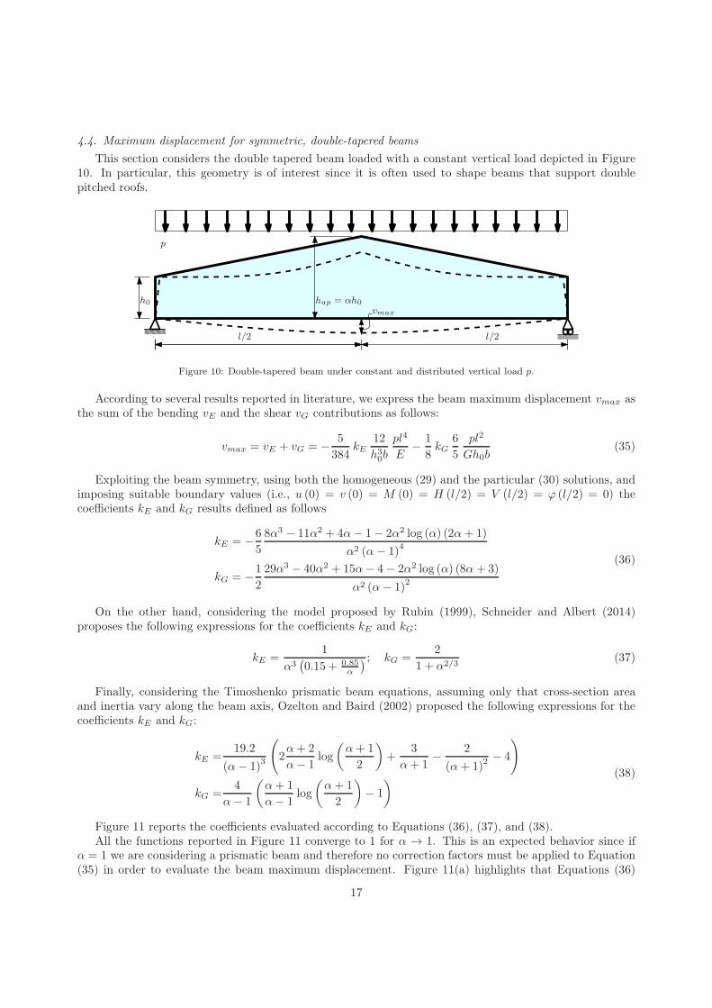
4.4. Maximum displacement for symmetric, double-tapered beams

This section considers the double tapered beam loaded with a constant vertical load depicted in Figure10. In particular, this geometry is of interest since it is often used to shape beams that support doublepitched roofs.

h0 hap = αh0

l/2l/2

vmax

p

Figure 10: Double-tapered beam under constant and distributed vertical load p.

According to several results reported in literature, we express the beam maximum displacement vmax asthe sum of the bending vE and the shear vG contributions as follows:

vmax = vE + vG = −5

384kE

12

h30b

pl4

E−

1

8kG

6

5

pl2

Gh0b(35)

Exploiting the beam symmetry, using both the homogeneous (29) and the particular (30) solutions, andimposing suitable boundary values (i.e., u (0) = v (0) = M (0) = H (l/2) = V (l/2) = ϕ (l/2) = 0) thecoefficients kE and kG results defined as follows

kE = −6

5

8α3 − 11α2 + 4α− 1− 2α2 log (α) (2α+ 1)

α2 (α− 1)4

kG = −1

2

29α3 − 40α2 + 15α− 4− 2α2 log (α) (8α+ 3)

α2 (α− 1)2

(36)

On the other hand, considering the model proposed by Rubin (1999), Schneider and Albert (2014)proposes the following expressions for the coefficients kE and kG:

kE =1

α3(0.15 + 0.85

α

) ; kG =2

1 + α2/3(37)

Finally, considering the Timoshenko prismatic beam equations, assuming only that cross-section areaand inertia vary along the beam axis, Ozelton and Baird (2002) proposed the following expressions for thecoefficients kE and kG:

kE =19.2

(α− 1)3

(2α+ 2

α− 1log

(α+ 1

2

)+

3

α+ 1−

2

(α+ 1)2 − 4

)

kG =4

α− 1

(α+ 1

α− 1log

(α+ 1

2

)− 1

) (38)

Figure 11 reports the coefficients evaluated according to Equations (36), (37), and (38).All the functions reported in Figure 11 converge to 1 for α → 1. This is an expected behavior since if

α = 1 we are considering a prismatic beam and therefore no correction factors must be applied to Equation(35) in order to evaluate the beam maximum displacement. Figure 11(a) highlights that Equations (36)

17

1 2 3 4 50

0.2

0.4

0.6

0.8

1

α

kE

Eq.(36)Eq.(37)Eq.(38)

(a) Coefficient kE evaluated for different values of α.

1 2 3 4 50.5

0.6

0.7

0.8

0.9

1

α

kG

Eq.(36)Eq.(37)Eq.(38)

(b) Coefficient kG evaluated for different values of α

Figure 11: Coefficients kE and kG for the evaluation of the maximum displacement, evaluated with different methods.

and (37) provide substantially identical evaluation of the coefficient kE . On the other hand, with respectto the proposed model, Equation (38) overestimates the bending contribution of values that could exceed100%. Figure 11(b) highlights that each model provides completely different evaluations of the coefficientkG. Furthermore, with respect to the model derived in this paper, both the formulas proposed in literatureunderestimates the shear contribution of values that could exceed the 40%.

The adoption of Equations (36) in engineering practice needs additional considerations on materialconstitutive law and rigorous validations that lie outside this paper’s aims. This specific aspect, as well asof other aspects of interest for practitioners, will be object of a further scientific paper.

5. Numerical examples

This section aims at providing further details about the obtained model capabilities. We consider twoexamples: (i) a tapered cantilever and (ii) an arch shaped beam. Both cases were already analyzed in(Auricchio et al., 2015) considering a more refined model.

5.1. Tapered Beam

We consider the symmetric tapered beam illustrated in Figure 12 (l = 10mm, h (0) = 1mm, andh (l) = 0.5mm) and we assume E = 105MPa and G = 4 · 104 MPa as material parameters. Moreover, thebeam is clamped in the initial cross-section A (0) and a concentrated load PPP = [0,−1] N acts on the finalcross-section A (l).

O

x

y

l

h (0)h (l)

P

Figure 12: Symmetric tapered beam: l = 10mm, h (0) = 1mm, h (l) = 0.5mm, P = 1N, E = 105 MPa, and G = 4 · 104 MPa.

18

Solving Equations (18), we obtain the following expressions for the generalized stresses

H (x) = 0; M (x) = x− 10; V (x) = 1 (39)

Figure 13 depicts the distributions of the stresses σx and τ in the cross-section A (0.5l). The label mod

indicates the stress distribution obtained using Equations (19a) and (21), whereas the label ref indicatesthe 2D FE solution, computed using the commercial software ABAQUS (Simulia, 2011), considering the full2D problem, and using a structured mesh of 7680×512 bilinear elements. Figure 13(b) allows to appreciate a

−60 −40 −20 0 20 40 60

−0.3

−0.2

−0.1

0

0.1

0.2

0.3

y[m

m]

σx [MPa]

mod

ref

(a) Horizontal stress σx cross-section distribution.

−1.334 −1.3338 −1.3336 −1.3334 −1.3332 −1.333

−0.3

−0.2

−0.1

0

0.1

0.2

0.3

y[m

m]

τ [MPa]

mod

ref

(b) Shear stress τ cross-section distribution.

Figure 13: Horizontal (Figure 13(a)) and shear (Figure 13(b)) stresses cross-section distributions, computed in the cross-sectionA (0.5l) for a symmetric tapered beam with a vertical load P = 1N applied in the final cross-section.

difference between the model and the reference solution, nevertheless the relative error magnitude is smallerthan 1 · 10−3.

Since H (x) = 0 therefore εHH (x) = χHH (x) = γHH (x) = 0; moreover, since c (x) = 0 also εM =εV = 0. Figure 14 depicts the plots of the generalized deformations χ (x) and γ (x). The curvature induced

0 2 4 6 8 10

0

5

10

15x 10

−4

χ(x

)[

mm

−1]

x [mm]

χVV (x)

χMM(x)

χ (x)

(a) Curvature χ (x) axial distribution.

0 2 4 6 8 10−1

0

1

2

3

4

5

6

x 10−5

γ(x

)[−

]

x [mm]

γV V (x)

γMM(x)

γ (x)

(b) Shear deformation γ (x) axial distribution.

Figure 14: Curvature (Figure 14(a)), and shear deformation (Figure 14(b)) axial distributions, evaluated for a tapered cantileverwith a shear load P = 1N applied in the final cross-section.

by vertical forces χV V (x) has a negligible magnitude with respect to the curvature induced by resultingbending moment χMM (x). On the other hand both shear deformations γMM (x) and γV V (x) have thesame order of magnitude and therefore both play a crucial role in determining the tapered beam’s behavior.

Figure 15 reports the beam displacements ϕ (x) and v (x). Table 1 reports the maximum vertical dis-placement evaluated with different models (i.e., the model proposed in this paper –indicated as Analyticalmodel–, the model developed by Auricchio et al. (2015) –indicated as ABL–, and the FE analysis software

19

0 2 4 6 8 100

0.002

0.004

0.006

0.008

0.01

0.012

ϕ(x

)[−

]

x [mm]

(a) Rotation ϕ (x) axial distribution.

0 2 4 6 8 10

−0.06

−0.05

−0.04

−0.03

−0.02

−0.01

0

v(x

)[m

m]

x [mm]

(b) Vertical displacement v (x) axial distribution.

Figure 15: Rotation (Figure 15(a)) and vertical displacements (Figure 15(b)) axial distributions, evaluated for a taperedcantilever with a shear load P = 1N applied in the final cross-section.

Beam model v (10) mm|v−vref ||vref |

Analytical model -0.0657826 1.064 ·10−3

ABL -0.0657294 2.541 ·10−4

2D solution (vref ) -0.0657127 -

Table 1: Mean value of the vertical displacement evaluated on the final cross-section and obtained considering different modelsfor a symmetric tapered cantilever with a vertical load P = 1N applied in the final cross-section.

ABAQUS –indicated as vref–). We note that all the models are accurate in predicting vertical displacement.Because it is more refined, ABL provides the most accurate prediction of vertical displacement whereas, be-ing less refined, the analytical model proposed in this paper is the less accurate. However, the analyticalmodel shows a good accuracy, acceptable in most engineering applications.

5.2. Arch Shaped Beam

We now consider the arch shaped beam depicted in Figure 16. The beam center-line and cross-sectionheight are defined as

c (x) := −1

100x2 +

1

10x; h (x) :=

1

50x2 −

1

5x+

3

5(40)

Moreover, the beam is clamped in the initial cross-section A (0) and loaded on the final cross-section A (l)

with a constant horizontal load distribution ttt|A(l) = [1, 0, 0]T N/mm.

Solving Equations (18), we obtain the following expressions for the generalized stresses

H (x) =3

5; M (x) =

3

5·

(−

1

100x2 +

1

10x

); V (x) = 0 (41)

Figure 17 depicts the cross-section distributions of the stresses σx and τ . The label mod indicates thestress distribution obtained using Equations (19a) and (21), whereas the label ref indicates the 2D ABAQUSsolution, computed considering the full 2D problem and using a structured mesh of 10240 × 256 bilinearelements. In order to exclude boundary effects, we consider the cross-section A (0.75l). We note the goodagreement between the Analytical model and the 2D FE solution.

Since V (x) = 0 therefore we have εV V (x) = χV V (x) = γV V (x) = 0. Figures 18(a), 18(c), and18(d) depict the generalized deformation ε0 (x), χ (x), and γ (x) respectively. We note that the horizontaldeformation induced by the bending moment εMM (x) has negligible magnitude compared with the hori-zontal deformation induced by the resulting horizontal stress εHH (x). Analogously, the curvature induced

20

q

O

x

y

l

∆h (0)

Figure 16: Arch shaped beam: l = 10mm, ∆ = 0.5mm, h (l) = h (0) = 0.6mm, q = 1N/mm, E = 105 MPa, and G =4 · 104 MPa.

−10 −5 0 5 10 15

0.1

0.15

0.2

0.25

y[m

m]

σx [MPa]

mod

ref

(a) Horizontal stress σx cross-section distribution.

−1.5 −1 −0.5 0 0.5

0.1

0.15

0.2

0.25

y[m

m]

τ [MPa]

mod

ref

(b) Shear stress τ cross-section distribution.

Figure 17: Horizontal (Figure 17(a)) and shear (Figure 17(b)) stresses cross-section distributions, computed in the cross-sectionA (0.75l) for an arch shaped beam with an horizontal load Q = 0.6N applied in the final cross-section.

by resulting horizontal stress χHH (x) has a negligible magnitude with respect to the curvature induced bybending moment χMM (x). On the other hand, both the shear deformations induced by resulting horizontalstress γHH (x) and bending moment γMM (x) have non-vanishing magnitudes.

Figure 18(b) shows the horizontal elongation induced by center-line rotation c′ (x)ϕ. This quantity istwo order of magnitude bigger than the horizontal deformation ε0 (x), and plays a central role in determiningthe horizontal displacements u.

Figure 19 reports the beam displacements u (x), ϕ (x), and v (x).Table 2 reports the maximum displacements v (l) and u (l) evaluated with different models. The reference

Beam model v (10) mm|v−vref ||vref |

u (10) mm|u−uref ||uref |

Analytical model 0.222569 5.979 ·10−4 0.0109037 5.598 ·10−4

ABL 0.222434 8.991 ·10−6 0.0108971 4.588 ·10−5

2D solution (vref , uref ) 0.222436 - 0.0108976 -

Table 2: Mean value of the vertical and horizontal displacements computed on the final cross-section and obtained consideringdifferent models for an arch shaped beam with an horizontal load Q = 0.6N applied in the final cross-section.

solutions vref and uref are calculated using the ABAQUS software. The numerical results confirm that theanalytical model is effective in predicting displacements despite it results less accurate than the model ABL.

21

0 2 4 6 8 100

1

2

3

4

5

6x 10

−5

ε[−

]

x [mm]

εHH (x)

εMM (x)

ε0 (x)

(a) Horizontal deformation ε0 (x) axial distribution.

0 2 4 6 8 10

0

0.5

1

1.5

2

2.5

3

3.5

4

x 10−3

c′(x

)ϕ[−

]

x [mm]

(b) Horizontal elongation induced by inclined center-linerotation c′ (x)ϕ.

0 2 4 6 8 10−18

−16

−14

−12

−10

−8

−6

−4

−2

0x 10

−3

χ(x

)[

mm

−1]

x [mm]

χHH(x)

χMM(x)

χ (x)

(c) Curvature χ (x) axial distribution.

0 2 4 6 8 10

−1

−0.5

0

0.5

1

x 10−5

γ(x

)[−

]

x [mm]

γHH(x)

γMM(x)

γ (x)

(d) Shear deformation γ (x) axial distribution.

Figure 18: Horizontal (Figure 18(a)), curvature (Figure 18(c)), shear (Figure 18(d)) deformations, and horizontal elongationinduced by inclined center-line rotation (Figure 18(b)) axial distributions evaluated for an arch shaped beam with an horizontalload Q = 0.6N applied in the final cross-section.

6. Conclusions

The modeling of a generic non-prismatic planar beam proposed in this paper was done through 4 main

steps

1. derivation of compatibility equations

2. derivation of equilibrium equations

3. stress representation

4. derivation of simplified constitutive relations

In particular, compatibility and equilibrium equations are derived considering a global Cartesian coordinate

system allowing the beam model to be expressed through simple ODEs. The stress representation takes

accurately into account the boundary equilibrium of the body, and is crucial in determining the model

effectiveness. The simplified constitutive relations need careful derivation and result in non-trivial equations.

The main conclusions highlighted by the derivation procedure and the discussion of practical examples

can be resumed as follows.

• The shear distribution depends not only on vertical resulting stress but also on horizontal resulting

stress and bending moment.

22

0 2 4 6 8 10

0

2

4

6

8

10

x 10−3

u(x

)[m

m]

x [mm]

(a) Horizontal displacement u (x).

0 2 4 6 8 10−0.045

−0.04

−0.035

−0.03

−0.025

−0.02

−0.015

−0.01

−0.005

0

ϕ(x

)[−

]

x [mm]

(b) Rotation ϕ (x).

0 2 4 6 8 100

0.05

0.1

0.15

0.2

v(x

)[m

m]

x [mm]

(c) Vertical displacement v (x) .

Figure 19: Horizontal (Figure 19(a)) and vertical (Figure 19(c)) displacements and rotation (Figure 19(b)) evaluated for anarch shaped beam with an horizontal load Q = 0.6N applied in the final cross-section.

• The complex geometry leads each generalized deformation to depend on all generalized stresses, in

contrast with prismatic beams.

• The proposed model allows the evaluation of homogeneous and particular solutions in simple cases of

practical interest.

• Example discussed in Section 5.2 highlights that non-prismatic beams could behave very differently

than prismatic ones, even if they are slender and with very smooth cross-section variations.

• Numerical examples demonstrate that the proposed model gives effective and accurate results for

complex geometries, so that the model is a promising tool for practitioners and researchers.

Further developments of the present work will include the application of the proposed model to more

realistic cases in particular to the simplified modeling of wood structures, as well as the generalization of

the proposed modeling procedure to 3D beams.

7. Acknowledgements

This work was partially funded by the Cariplo Foundation through the Projects iCardioCloud No. 2013-

1779 and SICURA No. 2013-1351 and by the Foundation Banca del Monte di Lombardia – Progetto

23

Professionalitá Ivano Benchi through the Project Enhancing Competences in Wooden Structure Design No.

1056.

References

Aminbaghai, M. and R. Binder (2006). Analytische Berechnung von Voutenstäben nach Theorie II. Ordnung unter Berück-sichtigung der M- und Q- Verformungen. Bautechnik 83, 770–776.

Arunakirinathar, K. and B. D. Reddy (1992). Solution of the equations for curved rods with constant curvature and torsion.Technical report, Centre for research in computational and applied mechanics, University of Cape Town.

Arunakirinathar, K. and B. D. Reddy (1993). Mixed finite element methods for elastic rods orf arbitrary geometry. NumerischeMathematik 64, 13–43.

Atkin, E. H. (1938). Tapered beams: suggested solutions for some typical aircraft cases. Aircraft Engineering 10, 371–374.Attarnejad, R., S. J. Semnani, and A. Shahaba (2010). Basic displacement functions for free vibration analysis of non-prismatic

Timoshenko beams. Finite Elements in Analysis and Design 46, 916–929.Auricchio, F., G. Balduzzi, and C. Lovadina (2015). The dimensional reduction approach for 2D non-prismatic beam modelling:

a solution based on Hellinger-Reissner principle. International Journal of Solids and Structures 15, 264–276.Balduzzi, G. (2013). Beam Models: Variational Derivation, Analytical and Numerical Solutions. Ph. D. thesis, Univeristà

degli Studi di Pavia.Balkaya, C. (2001). Behavior and modeling of nonprismatic members having T-sections. Journal of Structural Engineering 8,

940–946.Balkaya, C. and E. Citipitioglu (1997). Discusson of the paper “stiffness formulation for nonprismatic beam elements” by Arture

Tena-Colunga. Journal of structural engineering 123 (12), 1694–1695.Banerjee, J. R. and F. W. Williams (1985). Exact Bernoulli-Euler dynamic stiffness matrix for a range of tapered beams.

International Journal for Numerical Methods in Engineering 21 (12), 2289–2302.Banerjee, J. R. and F. W. Williams (1986). Exact Bernoulli-Euler static stiffness matrix for a range of tapered beam-columns.

International Journal for Numerical Methods in Engineering 23, 1615–1628.Beltempo, A. (2013). Derivation of non-prismatic beam models by a mixed variational method. Master’s thesis, Department

of civil engineering and architecture – University of Pavia.Beltempo, A., G. Balduzzi, G. Alfano, and F. Auricchio (2015). Analytical derivation of a general 2D non-prismatic beam

model based on the Hellinger-Reissner principle. Engineering Structures 101, 88–98.Boley, B. A. (1963). On the accuracy of the Bernoulli-Euler theory for beams of variable section. Journal of Applied Mechan-

ics 30, 374–378.Borri, M., G. L. Ghiringhelli, and T. Merlini (1992). Linear analysis of naturally curved and twisted anisotropic beams.

Composites Engineering 2 (5-7), 433–456.Bruhns, O. T. (2003). Advanced Mechanics of Solids. Springer.Capurso, M. (1971). Lezioni di Scienza delle Costruzioni. Pitagora Editrice Bologna.Cicala, P. (1939). Sulle travi di altezza variabile. Atti della Reale Accademia delle Scienze di Torino 74, 392–402.El-Mezaini, N., C. Balkaya, and E. Citipitioglu (1991). Analysis of frames with nonprismatic members. Journal of Structural

Engineering 117, 1573–1592.Franciosi, C. and M. Mecca (1998). Some finite elements for the static analysis of beams with varying cross section. Computers

and Structures 69, 191–196.Friedman, Z. and J. B. Kosmatka (1993). Exact stiffness matrix of a nonuniform beam - II bending of a Timoshenko beam.

Computers and Structures 49 (3), 545–555.Fung, Y. C. and A. Kaplan (1952). Buckling of low arches or curved beams of small curvature. National Advisory Commitee

for Aeronautics 2840, 1–75.Gimena, L., F. Gimena, and P. Gonzaga (2008a). Structural analysis of a curved beam element defined in global coordinates.

Engineering Structures 30, 3355–3364.Gimena, F. N., P. Gonzaga, and L. Gimena (2008b). 3D-curved beam element with varying cross-sectional area under generalized

loads. Engineering Structures 30, 404–411.Gross, D., W. Hauger, J. Schröder, W. A. Wall, and N. Rajapakse (2012). Statics. In Engineering Mechanics. Springer.Hodges, D. H., J. C. Ho, and W. Yu (2008). The effect of taper on section constants for in-plane deformation of an isotropic

strip. Journal of Mechanics of Materials and Structures 3, 425–440.Hodges, D. H., A. Rajagopal, J. C. Ho, and W. Yu (2010). Stress and strain recovery for the in-plane deformation of an

isotropic tapered strip-beam. Journal of Mechanics of Materials and Structures 5, 963–975.Kechter, G. E. and R. M.Gutkowski (1984). Double-tapered glulam beams: finite element analysis. Journal of Structural

Engineering 110, 978–991.Krahula, J. L. (1975). Shear formula for beams of variable cross section. AIAA (American Institute of Aeronautics and

Astronautics) journal 13, 1390–1391.Ozay, G. and A. Topcu (2000). Analysis of frames with non-prismatic members. Canadian Journal of Civil Engineering 27,

17–25.Ozelton, E. C. and J. A. Baird (2002). Timber designers’ manual. Blackwell Science Ltd.Paglietti, A. and G. Carta (2007). La favola del taglio efficace nella teoria delle travi di altezza variabile. In Atti del XVI

Congresso dell’Associazione italiana di meccanica teorica e applicata, Brescia, 11-14 Settembre 2007.

24

Paglietti, A. and G. Carta (2009). Remarks on the current theory of shear strength of variable depth beams. The open civilengineering journal 3, 28–33.

Popescu, B., D. H. Hodges, and C. E. S. Cesnik (2000). Obliqueness effects in asymptotic cross-sectional analysis of compositebeams. Computers and Structures 76, 533–543.

Portland Cement Associations (1958). Handbook of frame constants. Beam factor and moment coefficients for members ofvariable section. Portland Cement Associations.

Rajagopal, A. and D. H. Hodges (2014). Asymptotic approach to oblique cross-sectional analysis of beams. Journal of AppliedMechanics 81 (031015), 1–15.

Rajagopal, A., D. H. Hodges, and W. Yu (2012). Asymptotic beam theory for planar deformation of initially curved isotropicstrips. Thin-Walled Structures 50, 106–115.

Rajasekaran, S. and S. Padmanabhan (1989). Equations of curved beams. Journal of Engineering Mechanics 115, 1094–1111.Romano, F. (1996). Deflections of Timoshenko beam with varying cross-section. International Journal of Mechanical Sci-

ences 38 (8-9), 1017–1035.Rubin, H. (1999). Analytische Berechnung von Stäben mit linear veränderlicher Höhe unter Berücksichtigung von M-, Q- und

N- Verformungen. Stahlbau 68, 112–119.Sapountzakis, E. J. and D. G. Panagos (2008). Shear deformation effect in non-linear analysis of composite beams of variable

cross section. International Journal of Non-Linear Mechanics 43, 660–682.Schneider, K. and A. Albert (2014). Bautabellen für Ingenieure: mit Berechnungshinweisen und Beispielen. Bundesanzeiger

Verlag GmbH.Shooshtari, A. and R. Khajavi (2010). An efficent procedure to find shape functions and stiffness matrices of nonprismatic

Euler-Bernoulli and Timoshenko beam elements. European Journal of Mechanics, A/solids 29, 826–836.Simulia (2011). ABAQUS User’s and theory manuals - Release 6.11. Providence, RI, USA.: Simulia.Tena-Colunga, A. (1996). Stiffness formulation for nonprismatic beam elements. Journal of Structural Engineering 122,

1484–1489.Timoshenko, S. (1955). Elementary theory and problems. In Strength of materials. Krieger publishing company.Timoshenko, S. and J. N. Goodier (1951). Theory of Elasticity (Second ed.). McGraw-Hill.Timoshenko, S. P. and D. H. Young (1965). Theory of Structures. McGraw-Hill.Vogel, U. (1993). Berechnung von Bogentragwerken nach del elastizitätstheorie II: Ordnung. Chapter 3.5 in Stahlbau Handbuch

für Studium und Praxis Band 1, Teil A. Stahlbau-Verlagsgesellschaft mbH Köln 1, 211–226.Vu-Quoc, L. and P. Léger (1992). Efficient evaluation of the flexibility of tapered i-beams accounting for shear deformations.

International journal for numerical methods in engineering 33 (3), 553–566.Yu, W., D. H. Hodges, V. Volovoi, and C. E. Cesnik (2002). On Timoshenko-like modeling of initially curved and twisted

composite beams. International Journal of Solids and Structures 39, 5101–5121.

25