Non-convergence versusnon-conservation in effective
heat capacity methods forphase change problems
Zhen-Xiang Gong and Arun S. MujumdarDepartment of Chemical Engineering, McGill University,
Montreal, Quebec, Canada
Nomenclature
IntroductionTo handle moving interfaces numerically in solving melting and solidificationproblems, two types of solution techniques have been developed. One is the timedependent grid method and the other is the fixed grid method. Because of theirconceptual simplicity and ease of implementation, fixed grid approaches havefound wide application. The essential feature of fixed grid approaches is that
c = specific heatceff = effective specific heat (λ /∆T )[C ] = heat capacity matrix[CIJ ] = elements of heat capacity matrixF = heat load vectorFI = elements of heat load vectorh = convection heat transfer
coefficientH = enthalpyk = thermal conductivity[K] = conductance matrixKIJ = elements of conductance matrixn = outward normal of boundaryNI,NJ = shape functionq = heat flux due to conductionQ = rate of internal heat generation T = temperatureTf = ambient temperatureTi = initial temperatureTm = melting temperatureTmn = lower limit of melting
temperature (Tm–0.5∆T)
Tmp = upper limit of melting temperature (Tm+0.5∆T)
t = timex,y,z = space co-ordinates
Greek symbols∆t = time step∆T = phase change temperature
Superscriptse = element i = ith iteration n = nth time step
SubscriptsI,J = node number of an elementl = liquid phases = solid phaset = time tt + ∆t = time t + ∆t
Note: The symbols defined above are subject to alteration on occasion
Z.-X. Gong gratefully acknowledges the financial support of the Canadian InternationalDevelopment Agency (CIDA) and McGill University in the form of a McGill/CIDA Fellowship.Research support of the Natural Science and Engineering Council of Canada as well as theExergex Corporation is also acknowledged.
Received June 1995Revised April 1996
International Journal of NumericalMethods for Heat & Fluid Flow
the latent heat evolution is accounted for in the governing equation by definingeither an enthalpy, or an effective specific heat, or a heat source. Consequently,the numerical solution can be carried out on a space grid that remains fixedthroughout the calculation process.
In the original effective heat capacity method the latent heat effect isapproximated by a large effective heat capacity over a small temperaturerange[1]. This approach is simple in concept and easy to implement.Unfortunately, however, it is so sensitive to the choice of the phase changetemperature interval and time integration scheme that in some cases the correctsolution or even a solution cannot be obtained owing to non-convergence causedby the abrupt change of specific heat at the interface. Many improved versionsof this approach have been reported over the last two decades (e.g. Comini etal.[2], Morgan et al.[3], Guidice et al.[4], Lemmon[5], Pham[6] and Comini etal.[7]). These improved versions have been well established and are effective insolving a wide range of conduction phase change problems. However, in theauthors’ experience, non-convergence sometimes occurs when these approachesare implemented with implicit iterative time integration schemes and a largetime step is used, e.g. the Lemmon scheme[5]. Swaminathan and Voller[8]reported a source based method to deal with phase change problems. Theirscheme is strictly conservative and computationally efficient.
In this paper, the cause and cure of non-convergence in effective heat capacitymethods are presented. Based on the energy conservation law, the transientsemi-discretized governing equation based on the original effective heatcapacity method is reformulated.
Mathematical formulationLet us take the original effective heat capacity method[1] for illustration. Thegoverning equation for phase change heat conduction based on this method canbe described by:
(1)
in which
(2)
Finite element formulationAfter spacewise discretization of equation (1), subject to the boundary conditionof the third kind (convection boundary condition), viz.
Heat capacitymethods
567
(3)
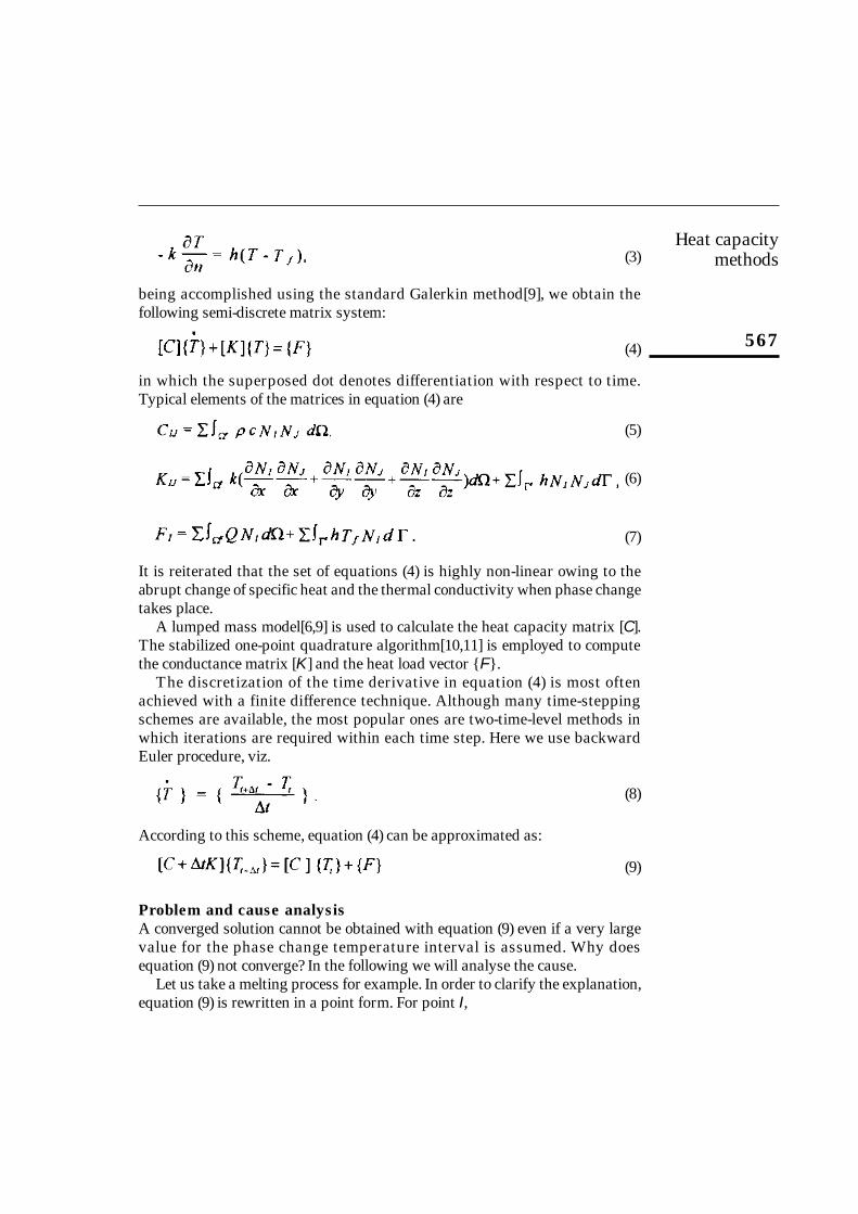
being accomplished using the standard Galerkin method[9], we obtain thefollowing semi-discrete matrix system:
(4)
in which the superposed dot denotes differentiation with respect to time.Typical elements of the matrices in equation (4) are
(5)
(6)
(7)
It is reiterated that the set of equations (4) is highly non-linear owing to theabrupt change of specific heat and the thermal conductivity when phase changetakes place.
A lumped mass model[6,9] is used to calculate the heat capacity matrix [C].The stabilized one-point quadrature algorithm[10,11] is employed to computethe conductance matrix [K] and the heat load vector F.
The discretization of the time derivative in equation (4) is most oftenachieved with a finite difference technique. Although many time-steppingschemes are available, the most popular ones are two-time-level methods inwhich iterations are required within each time step. Here we use backwardEuler procedure, viz.
(8)
According to this scheme, equation (4) can be approximated as:
(9)
Problem and cause analysisA converged solution cannot be obtained with equation (9) even if a very largevalue for the phase change temperature interval is assumed. Why doesequation (9) not converge? In the following we will analyse the cause.
Let us take a melting process for example. In order to clarify the explanation,equation (9) is rewritten in a point form. For point I,
HFF7,6
568
(10)
According to the implicit scheme rules, the values of Cl, KIJ, and FI should beupdated with the latest temperature T i–1
t+∆t. Assume point I enters phase changefrom solid state during the time interval, t to t + ∆t, and T i–1
t+∆t < Tmn (Tm –0.5∆T)and T i
t+∆t > Tmn. At iteration i,cI takes on the value of cs and there is T it+∆t > Tmn.
T it+∆t has two possible situations. One is Tmn < T i
t+∆t < Tmp (Tm + 0.5∆T) and theother is T i
t+∆t > Tmp. The latter case occurs when the phase change temperatureinterval is very small or the time step is very large or both. For the latter casephase change is stepped over in an iteration and latent heat effect is not takeninto account. A false solution is therefore reached.
For the former case the following will happen. At iteration i + 1, cI takes onthe value of ceff (λ/∆T) and CI becomes a very large number correspondinglysince ceff is in general a very large value. Compared with this large value of CI,relative contributions of the other terms to equation (10) can be neglected.Therefore, equation (10) becomes:
(11)
and therefore, T i+1t+∆t ≈ Tt < Tmn. In this case T i+1
t+∆t is dragged back to atemperature in solid state, and then an iteration i+2, cI takes on the value of csagain. This results in Tmn < Ti+2
t+∆t < Tmp. At iteration i+3, the same situation asiteration i+1 occurs. This explains why a converged solution can never beobtained.
Even if the phase change temperature interval is assumed to be a very largevalue, ceff is still in general tens, or even hundreds, of times larger than cs or cl.Therefore, such temperature oscillations as described above cannot be avoided.
What is the true value of temperature T i+1t+∆t? Since the real process is that at
iteration i the control volume has already entered the melting state, T i+1t+∆t should
be in the the range of the melting temperature interval, i.e. Tmn < T i+1t+∆t < Tmp.
Why do the above mentioned temperature oscillations occur? This is owingto the non-conservative behaviour caused by the abrupt change of specificheat in the time interval of t to t +∆t. In the following, we will reformulate theheat transfer process based on the basic energy conservation law. After thecorrect formulations are obtained, the non-conservation behaviour will beseen clearly.
In the Lemmon scheme[5], the effective specific heat is calculated as follows:
(12)
Similar temperature oscillation in the Lemmon scheme to that described aboveoccasionally occurs as it is implemented with an implicit iteration timeintegration scheme and the time step exceeds a certain limit. This will be shownin the illustrative examples.
Heat capacitymethods
569
A conservative schemeHere let us model a one-dimensional melting process for illustration. Assume acontrol volume dx (see Figure 1) is in solid state at time t, and at time t+∆t it hasentered molten state. During the time interval ∆t the net thermal energy flowinginto the control volume by conduction is:
(13)
The thermal energy is absorbed by the material heat capacity and there is,therefore, a temperature rise in the control volume. Thermal energy absorbedby the control volume (see Figure 2) is:
(14)
According to the energy conservation law we obtain:
(15)
Figure 1.Physical model
x
x + dx
q q +∂q∂x dx
Figure 2.Illustration of the heattransfer process in the
H-T curve
t + ∆t
t
H
TTmn Tmp
HFF7,6
570
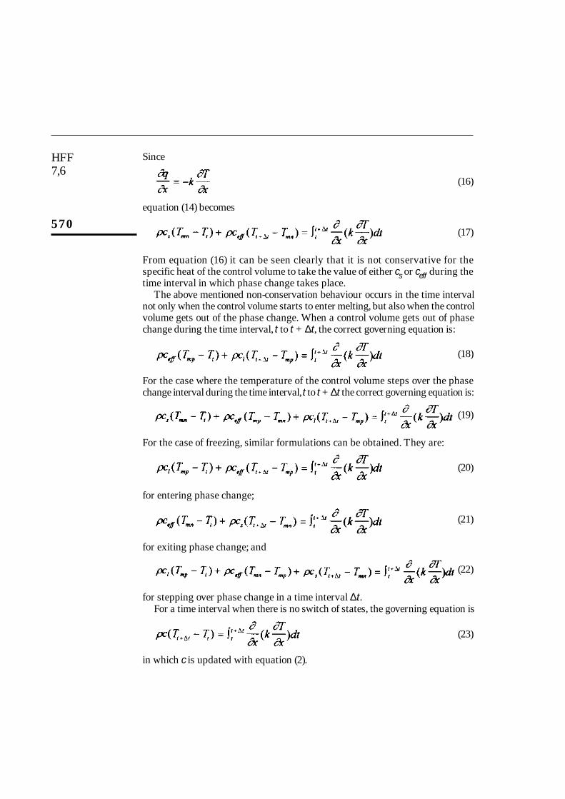
Since
(16)
equation (14) becomes
(17)
From equation (16) it can be seen clearly that it is not conservative for thespecific heat of the control volume to take the value of either cs or ceff during thetime interval in which phase change takes place.
The above mentioned non-conservation behaviour occurs in the time intervalnot only when the control volume starts to enter melting, but also when the controlvolume gets out of the phase change. When a control volume gets out of phasechange during the time interval, t to t + ∆t, the correct governing equation is:
(18)
For the case where the temperature of the control volume steps over the phasechange interval during the time interval, t to t + ∆t the correct governing equation is:
(19)
For the case of freezing, similar formulations can be obtained. They are:
(20)
for entering phase change;
(21)
for exiting phase change; and
(22)
for stepping over phase change in a time interval ∆t.For a time interval when there is no switch of states, the governing equation is
(23)
in which c is updated with equation (2).
Heat capacitymethods
571
The reformulated governing equations are exactly conservative. As will beseen in the test examples, temperature oscillation which results in non-convergence is completely eliminated and the new scheme has no limitation onselection of the phase change temperature interval.
The Newton-Raphson method is used to solve the resulting algebraicequation system. The convergence criteria selected are that the Cartesian normsof both the increment of temperature rate and the residual of the algebraicequation system are each less than a small constant, e.g. 1.0 × 10⁻⁶.
ImplementationTaking the melting case for illustration, four cases are required to distinguishthe implementation of the newly proposed scheme.
(1) if Tt < Tmn and T it+∆t < Tmn or Tt > Tmp and T i
t+∆t > Tmp, equation (23) isused;
(2) if Tt < Tmn and Tmn < T it+∆t < Tmp, equation (17) is used;
(3) If Tmn < Tt < Tmp and T it+∆t > Tmp, equation (18) is used;
(4) if Tt < Tmn and T it+∆t < Tmp equation (19) is used.
No special treatment is required in the solution iteration process except forchecking the temperature of the element nodes at each iteration and adoptingthe corresponding equation according to the temperature of the element node.
Illustrative examplesTo demonstrate the accuracy and efficiency of the new conservative scheme,solutions of four illustrative problems are presented. All the computations werecarried out by a Pentium 100 MHz.
Problem 1: Solidification of a semi-infinite slab of a liquid – constant thermalpropertiesA liquid initially at a uniform temperature, 10°C, which is above its freezingpoint (0°C) is confined to a half-space x > 0. At time t = 0, the boundary surfaceat x = 0 is lowered to a temperature, –20°C and maintained at this temperaturefor t > 0. The thermophysical properties are as follows:
Two-dimensional elements are utilized to solve this problem although it isphysically one-dimensional. The finite element mesh is displayed in Figure 3 inwhich BC = 1.0m. A phase change temperature interval of 1.0 × 10⁻¹⁰ is used forthe computations in this test problem.
Figure 3.Finite element mesh
A D
B C
14
13
HFF7,6
572
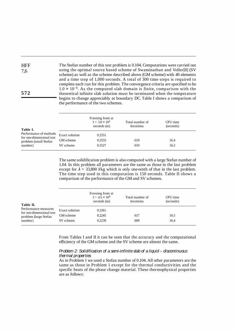
The Stefan number of this test problem is 0.104. Computations were carried outusing the optimal source based scheme of Swaminathan and Voller[8] (SVscheme) as well as the scheme described above (GM scheme) with 40 elementsand a time step of 1,000 seconds. A total of 300 time steps is required tocomplete each run for this problem. The convergence criteria are specified to be1.0 × 10–6. As the computed slab domain is finite, comparison with thetheoretical infinite slab solution must be terminated when the temperaturebegins to change appreciably at boundary DC. Table I shows a comparison ofthe performance of the two schemes.
The same solidification problem is also computed with a large Stefan number of1.04. In this problem all parameters are the same as those in the last problemexcept for λ = 33,800 J/kg which is only one-tenth of that in the last problem.The time step used in this computation is 150 seconds. Table II shows acomparison of the performance of the GM and SV schemes.
From Tables I and II it can be seen that the accuracy and the computationalefficiency of the GM scheme and the SV scheme are almost the same.
Problem 2: Solidification of a semi-infinite slab of a liquid – discontinuousthermal propertiesAs in Problem 1 we used a Stefan number of 0.104. All other parameters are thesame as those in Problem 1 except for the thermal conductivities and thespecific heats of the phase change material. These thermophysical propertiesare as follows:
Freezing front att = 3.0 × 10⁵ Total number of CPU timeseconds (m) iterations (seconds)
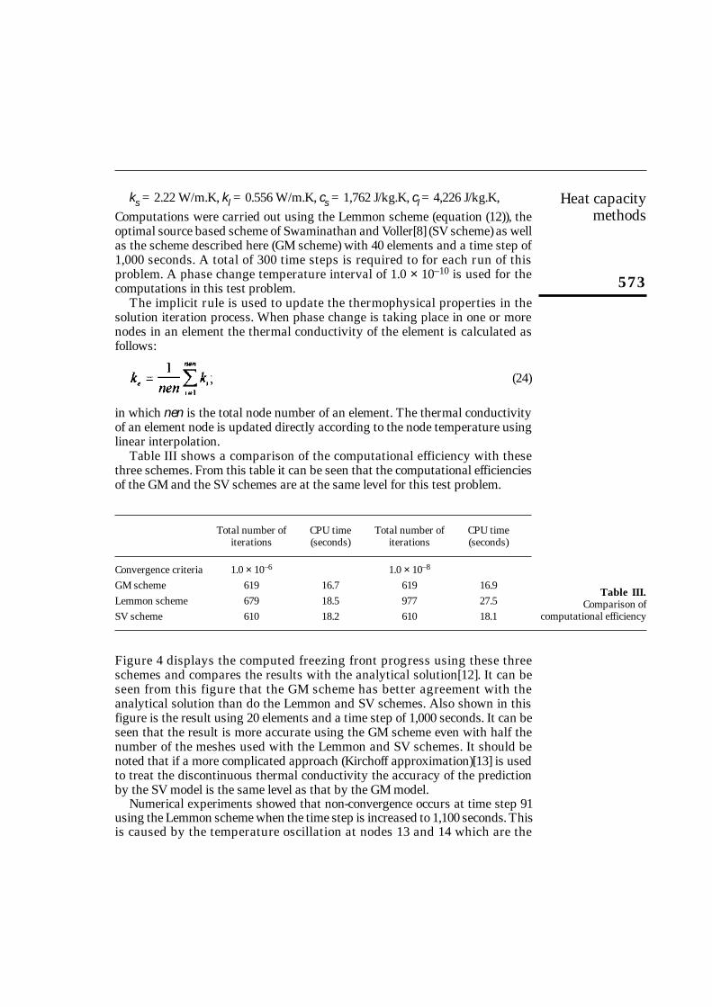
ks = 2.22 W/m.K, kl = 0.556 W/m.K, cs = 1,762 J/kg.K, cl = 4,226 J/kg.K,Computations were carried out using the Lemmon scheme (equation (12)), theoptimal source based scheme of Swaminathan and Voller[8] (SV scheme) as wellas the scheme described here (GM scheme) with 40 elements and a time step of1,000 seconds. A total of 300 time steps is required to for each run of thisproblem. A phase change temperature interval of 1.0 × 10⁻¹⁰ is used for thecomputations in this test problem.
The implicit rule is used to update the thermophysical properties in thesolution iteration process. When phase change is taking place in one or morenodes in an element the thermal conductivity of the element is calculated asfollows:
(24)
in which nen is the total node number of an element. The thermal conductivityof an element node is updated directly according to the node temperature usinglinear interpolation.
Table III shows a comparison of the computational efficiency with thesethree schemes. From this table it can be seen that the computational efficienciesof the GM and the SV schemes are at the same level for this test problem.
Figure 4 displays the computed freezing front progress using these threeschemes and compares the results with the analytical solution[12]. It can beseen from this figure that the GM scheme has better agreement with theanalytical solution than do the Lemmon and SV schemes. Also shown in thisfigure is the result using 20 elements and a time step of 1,000 seconds. It can beseen that the result is more accurate using the GM scheme even with half thenumber of the meshes used with the Lemmon and SV schemes. It should benoted that if a more complicated approach (Kirchoff approximation)[13] is usedto treat the discontinuous thermal conductivity the accuracy of the predictionby the SV model is the same level as that by the GM model.
Numerical experiments showed that non-convergence occurs at time step 91using the Lemmon scheme when the time step is increased to 1,100 seconds. Thisis caused by the temperature oscillation at nodes 13 and 14 which are the
Total number of CPU time Total number of CPU timeiterations (seconds) iterations (seconds)
junctions of elements 6 and 7. The temperatures at nodes 13 and 14 oscillate from0.5007 to –0.6626 iteration by iteration and convergence cannot be reached. Aninsight into the computation process determined that when the temperaturesoscillate from 0.5007 to –0.6626 the effective specific heat of element 6 oscillatesfrom 106,562.6 J/kg.K to 4,226 J/kg.K (specific heat of the liquid phase) and thatof element 7 from 1,762 J/kg.K (specific heat of the solid phase) to 159,043.6J/kg.K. The oscillation of the element specific heat results in a jump in the valueof the effective specific heat of nodes 13 and 14 (from 54,162.3 J/kg.K to 81,634.8J/kg.K). This jump leads to non-conservation of the final algebraic equations forpoints 13 and 14. A similar explanation can be given for such observations madeon the original effective heat capacity method described previously.
Numerical experiments also showed that convergence can be reached evenwith a very large time step, e.g. 3,000 seconds, and that the accuracy does notdegrade with the new conservative scheme. From Figure 4 it can be seen thatthe results using a time step of 3,000 seconds are in very good agreement withthe analytical solution.
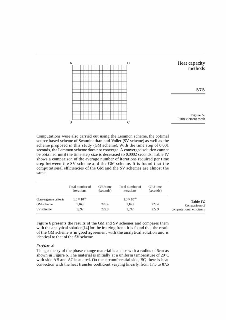
Problem 3. Solidification of a corner regionThe corner region of a liquid body extending in the positive x and y-directions isfrozen by bringing the surface temperature to –1.0°C at time t = 0. Thethermophysical properties are ks = kl = 1.0 W/m.K, cs = cl = 1.0 J/kg.K, ρ = 1.0kg/m3, Tm = 0°C, λ = 0.25 J/kg and the initial condition is Ti = 0.3°C. The phasechange temperature interval is specified to be 1.0× 10⁻¹⁰ K. 20 × 20 elements witha time step of 0.001 second are employed. A total of 500 time steps is required tocomplete each run for this problem. The finite element mesh is shown in Figure 5.
Figure 4.Comparison of thecomputed interfaceposition with theanalytical solution
Computations were also carried out using the Lemmon scheme, the optimalsource based scheme of Swaminathan and Voller (SV scheme) as well as thescheme proposed in this study (GM scheme). With the time step of 0.001seconds, the Lemmon scheme does not converge. A converged solution cannotbe obtained until the time step size is decreased to 0.0002 seconds. Table IVshows a comparison of the average number of iterations required per timestep between the SV scheme and the GM scheme. It is found that thecomputational efficiencies of the GM and the SV schemes are almost thesame.
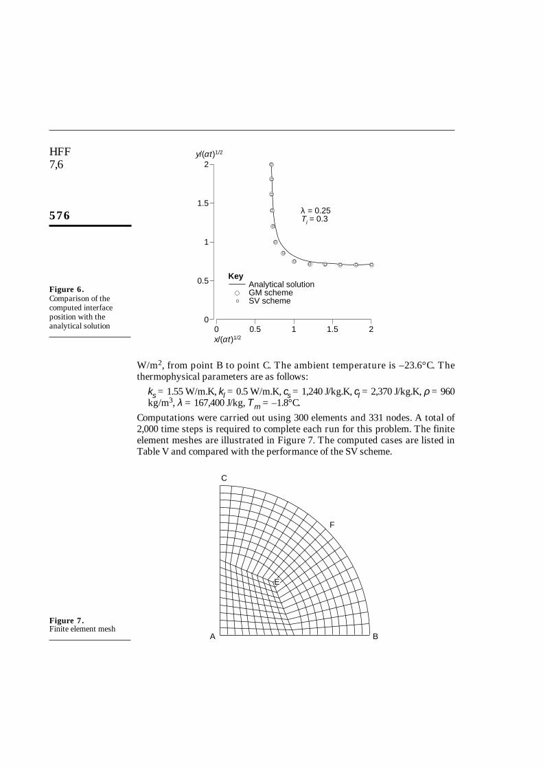
Figure 6 presents the results of the GM and SV schemes and compares themwith the analytical solution[14] for the freezing front. It is found that the resultof the GM scheme is in good agreement with the analytical solution and isidentical to that of the SV scheme.
Problem 4The geometry of the phase change material is a slice with a radius of 5cm asshown in Figure 6. The material is initially at a uniform temperature of 20°Cwith side AB and AC insulated. On the circumferential side, BC, there is heatconvection with the heat transfer coefficient varying linearly, from 17.5 to 87.5
Figure 5.Finite element mesh
A D
B C
Total number of CPU time Total number of CPU timeiterations (seconds) iterations (seconds)
Computations were carried out using 300 elements and 331 nodes. A total of2,000 time steps is required to complete each run for this problem. The finiteelement meshes are illustrated in Figure 7. The computed cases are listed inTable V and compared with the performance of the SV scheme.
Figure 6.Comparison of thecomputed interfaceposition with theanalytical solution
2
1.5
1
0.5
00 0.5 1 1.5 2
KeyAnalytical solutionGM schemeSV scheme
x/(at )1/2α
y/(at )1/2α
λ = 0.25Ti = 0.3
Figure 7.Finite element mesh
C
A B
F
E
Heat capacitymethods
577
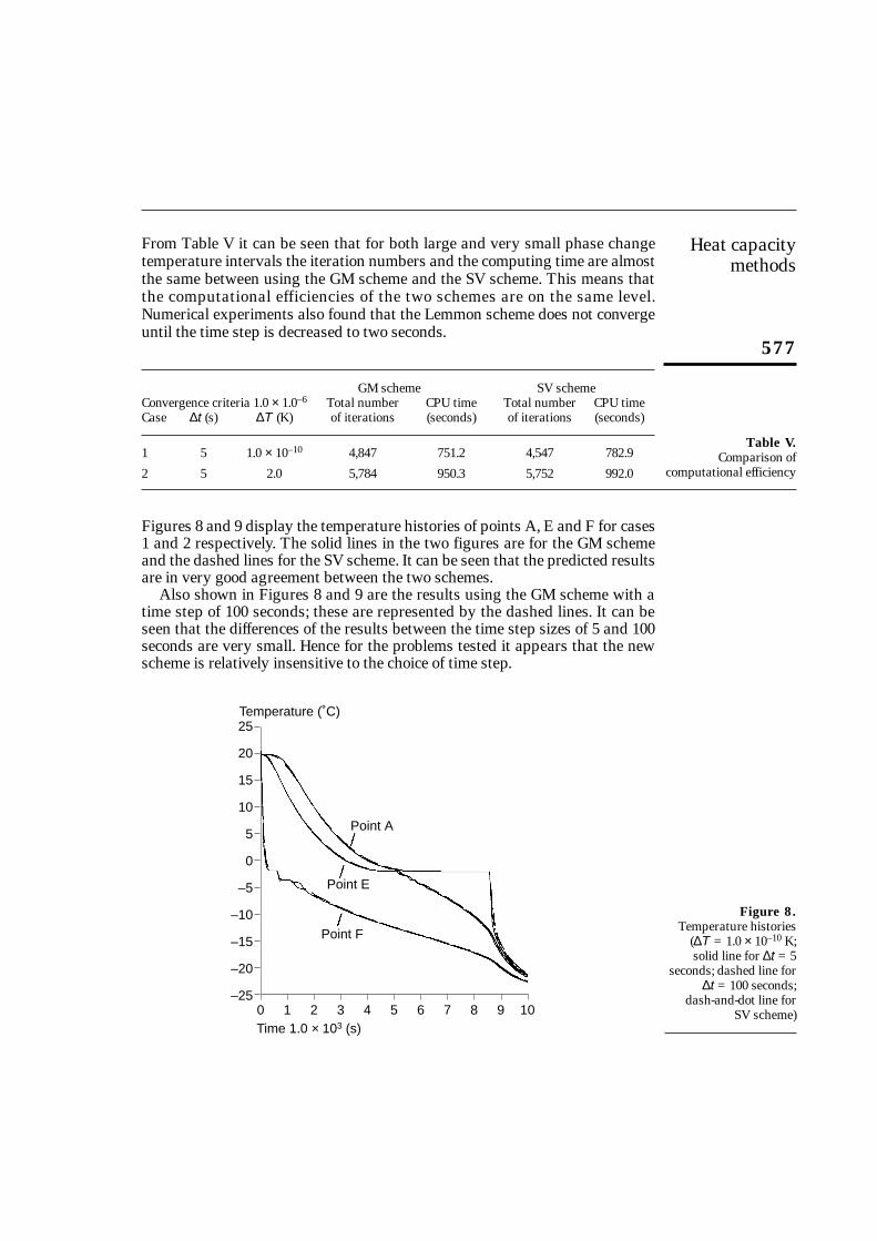
From Table V it can be seen that for both large and very small phase changetemperature intervals the iteration numbers and the computing time are almostthe same between using the GM scheme and the SV scheme. This means thatthe computational efficiencies of the two schemes are on the same level.Numerical experiments also found that the Lemmon scheme does not convergeuntil the time step is decreased to two seconds.
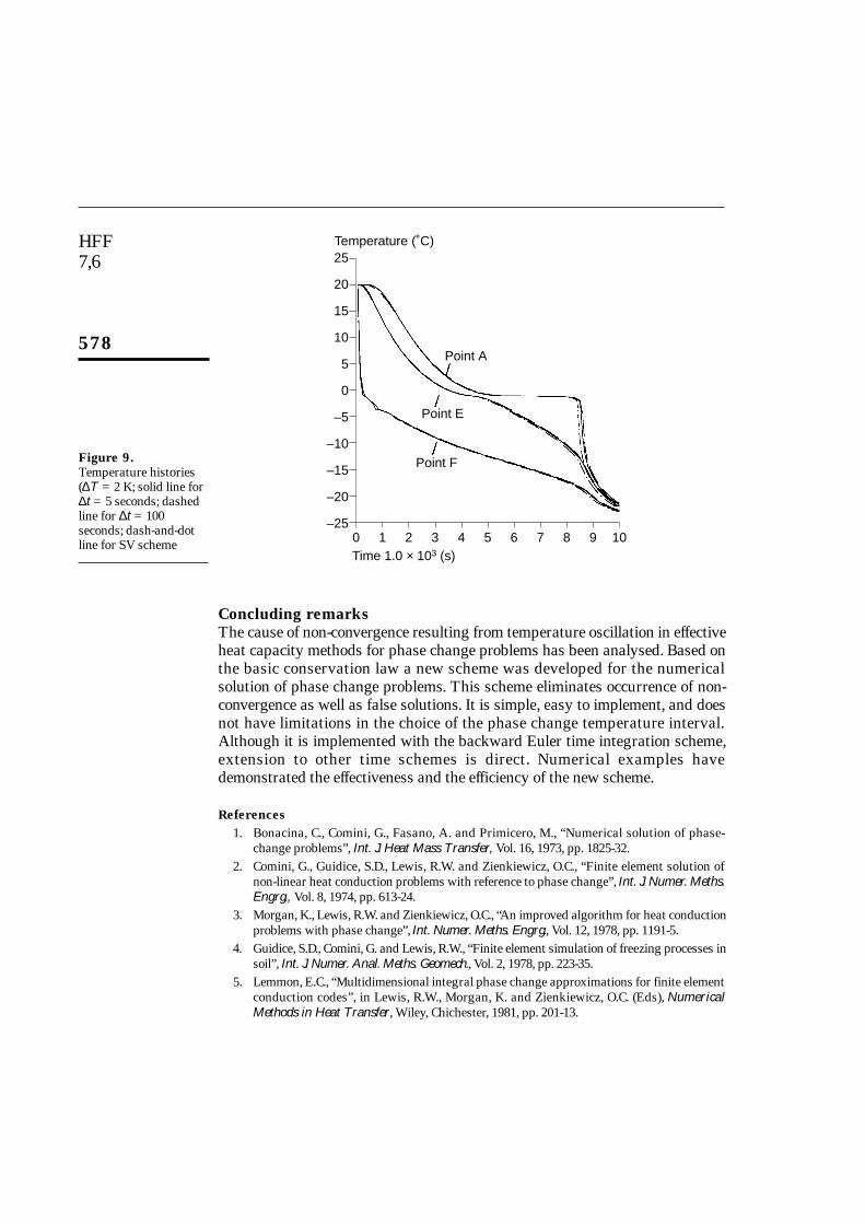
Figures 8 and 9 display the temperature histories of points A, E and F for cases1 and 2 respectively. The solid lines in the two figures are for the GM schemeand the dashed lines for the SV scheme. It can be seen that the predicted resultsare in very good agreement between the two schemes.
Also shown in Figures 8 and 9 are the results using the GM scheme with atime step of 100 seconds; these are represented by the dashed lines. It can beseen that the differences of the results between the time step sizes of 5 and 100seconds are very small. Hence for the problems tested it appears that the newscheme is relatively insensitive to the choice of time step.
GM scheme SV schemeConvergence criteria 1.0 × 1.0–6 Total number CPU time Total number CPU timeCase ∆t (s) ∆T (K) of iterations (seconds) of iterations (seconds)
1 5 1.0 × 10⁻¹⁰ 4,847 751.2 4,547 782.9
2 5 2.0 5,784 950.3 5,752 992.0
Table V.Comparison of
computational efficiency
Figure 8.Temperature histories
(∆T = 1.0 × 10⁻¹⁰ K;solid line for ∆t = 5
seconds; dashed line for∆t = 100 seconds;
dash-and-dot line for SV scheme)
25
20
15
10
5
0
–5
–10
–15
–20
–250 1 2 3 4 5 6 7 8 9 10
Temperature (˚C)
Time 1.0 × 10³ (s)
Point A
Point E
Point F
HFF7,6
578
Concluding remarksThe cause of non-convergence resulting from temperature oscillation in effectiveheat capacity methods for phase change problems has been analysed. Based onthe basic conservation law a new scheme was developed for the numericalsolution of phase change problems. This scheme eliminates occurrence of non-convergence as well as false solutions. It is simple, easy to implement, and doesnot have limitations in the choice of the phase change temperature interval.Although it is implemented with the backward Euler time integration scheme,extension to other time schemes is direct. Numerical examples havedemonstrated the effectiveness and the efficiency of the new scheme.
References1. Bonacina, C., Comini, G., Fasano, A. and Primicero, M., “Numerical solution of phase-
change problems”, Int. J. Heat Mass Transfer, Vol. 16, 1973, pp. 1825-32.2. Comini, G., Guidice, S.D., Lewis, R.W. and Zienkiewicz, O.C., “Finite element solution of
non-linear heat conduction problems with reference to phase change”, Int. J. Numer. Meths.Engrg., Vol. 8, 1974, pp. 613-24.
3. Morgan, K., Lewis, R.W. and Zienkiewicz, O.C., “An improved algorithm for heat conductionproblems with phase change”, Int. Numer. Meths. Engrg., Vol. 12, 1978, pp. 1191-5.
4. Guidice, S.D., Comini, G. and Lewis, R.W., “Finite element simulation of freezing processes insoil”, Int. J. Numer. Anal. Meths. Geomech., Vol. 2, 1978, pp. 223-35.
5. Lemmon, E.C., “Multidimensional integral phase change approximations for finite elementconduction codes”, in Lewis, R.W., Morgan, K. and Zienkiewicz, O.C. (Eds), NumericalMethods in Heat Transfer, Wiley, Chichester, 1981, pp. 201-13.
Figure 9.Temperature histories(∆T = 2 K; solid line for∆t = 5 seconds; dashedline for ∆t = 100seconds; dash-and-dotline for SV scheme
25
20
15
10
5
0
–5
–10
–15
–20
–250 1 2 3 4 5 6 7 8 9 10
Temperature (˚C)
Time 1.0 × 10³ (s)
Point A
Point E
Point F
Heat capacitymethods
579
6. Pham, Q.T., “The use of lumped capacitance in the finite-element solution of heat conductionproblems with phase change”, Int. J. Heat Mass Transfer, Vol. 29, 1986, pp. 285-91.
7. Comini, G., Guidice, S.D. and Saro, O., “A conservative algorithm for multidimensionalconduction phase change”, Int. Numer. Meths. Engrg., Vol. 30, 1990, pp. 697-709.
8. Swaminathan, C.R. and Voller, V.R., “On the enthalpy method”, Int. Num. Meth. Heat FluidFlow, Vol. 3, 1993, pp. 233-44.
9. Zienkiewicz, O.C. and Taylor, R.L., The Finite Element Method, 4th ed., Vol. 1, McGraw-Hill,London, 1989.
10. Liu, W.K. and Belytschko, T., “Efficient linear and non-linear heat conduction with aquadrilateral element”, Int. J. Numer. Meths. Engrg., Vol. 20, 1984, pp. 931-48.
11. Gong, Z.X. and Mujumdar, A.S., “A simultaneous iteration procedure for the finite elementsolution of the enthalpy model for phase change heat conduction problems”, Int. J. Num.Meth. Heat Fluid Flow, Vol. 5, 1994, pp. 589-600.
12. Luikov, A.V., Analytical Heat Diffusion Theory, Academic Press, New York, NY, 1968.13. Voller, V.R. and Swaminathan, C.R., “Treatment of discontinuous thermal conductivity in
control-volume solutions of phase-change problems”, Numerical Heat Transfer, Part B,Vol. 24, 1993, pp. 161-80.
14. Budhia, H. and Kreith, F., “Heat transfer with melting or freezing in a wedge”, Int. J. HeatMass Transfer, Vol. 16, 1973, pp. 195-211.