1 1 1 Abstract Nonlinear Adjustment to Purchasing Power Parity in the post-Bretton Woods Era Christopher F. Baum Department of Economics Boston College John T. Barkoulas Department of Economics and Finance Louisiana Tech University Mustafa Caglayan Department of Economics and Finance University of Durham, UK This paper models the dynamics of adjustment to long-run PPP over the post-Bretton Woods period in a nonlinear framework consistent with the presence of frictions in international trade. We estimate exponential smooth transition autoregressive (ESTAR) models of deviations from PPP, which are obtained using the Johansen cointegration method, for both CPI- and WPI- based measures and a broad set of U.S. trading partners. In several cases, we nd clear evidence of a mean-reverting dynamic process for sizable deviations from PPP, with the equilibrium ten- dency varying nonlinearly with the magnitude of disequilibrium. Analysis of impulse response functions also supports a nonlinear dynamic structure, but convergence to long-run PPP in the post-Bretton Woods era is very slow. JEL: F32, C22. Keywords: purchasing power parity, ESTAR, cointegration. Corresponding author: Christopher F. Baum, Department of Economics, Boston College, Chestnut Hill, MA 02467 USA, Tel: 617-552-3673, fax 617-552-2308, e-mail: [email protected].
Transcript
1
1
1
Abstract
Nonlinear Adjustment to PurchasingPower Parity in the post-Bretton Woods
Era
Christopher F. BaumDepartment of Economics
Boston College
John T. BarkoulasDepartment of Economics and Finance
Louisiana Tech University
Mustafa CaglayanDepartment of Economics and Finance
University of Durham, UK
This paper models the dynamics of adjustment to long-run PPP over the post-Bretton Woods
period in a nonlinear framework consistent with the presence of frictions in international trade.
We estimate exponential smooth transition autoregressive (ESTAR) models of deviations from
PPP, which are obtained using the Johansen cointegration method, for both CPI- and WPI-
based measures and a broad set of U.S. trading partners. In several cases, we 1nd clear evidence
of a mean-reverting dynamic process for sizable deviations from PPP, with the equilibrium ten-
dency varying nonlinearly with the magnitude of disequilibrium. Analysis of impulse response
functions also supports a nonlinear dynamic structure, but convergence to long-run PPP in the
post-Bretton Woods era is very slow.
JEL: F32, C22. Keywords: purchasing power parity, ESTAR, cointegration.
Corresponding author: Christopher F. Baum, Department of Economics, Boston College,Chestnut Hill, MA 02467 USA, Tel: 617-552-3673, fax 617-552-2308, e-mail: [email protected].
1
2
3
4
1
2
3
4
1 Introduction
Relative PPP, which is implied by absolute PPP, states that the growth rate in the nominal exchange rate equalsthe differential between the growth rates in home and foreign price indices.
See Rogoff (1996) and Froot and Rogoff (1995) for a review of the literature on PPP.Employing an alternative multivariate unit-root test where the null hypothesis is nonstationarity of at least one of
the series under consideration, Taylor and Sarno (1998) 1nd strong support for mean reversion in a panel of CPI-basedU.S. dollar exchange rates of the G5 countries. However, their evidence is not supportive of mean reversion for GNPdeBator- and PPICbased real exchange rates for the same panel of countries. Taylor and Sarno also point to a numberof pitfalls when using panel unit-root tests.
See Higgins and Zakrajsek (1999) for evidence contrary to that of OFConnellFs.
The doctrine of purchasing power parity (PPP) in its absolute form states that a com-
mon basket of goods, when quoted in the same currency, costs the same in all countries.
The parity condition rests on the assumption of perfect inter-country commodity arbi-
trage and is a central building block of many theoretical and empirical models of exchange
rate determination. Due to factors like transaction costs, taxation, subsidies, actual or
threatened trade restrictions, the existence of nontraded goods, imperfect competition,
foreign exchange market interventions, and the differential composition of market baskets
and price indices across countries, one may expect PPP to be valid only in the long-run.
Empirical studies over long periods have supported long-run PPP (Diebold et al.
(1991), Taylor (1996), Michael et al. (1997)). However, results are mixed when the
recent Boating-rate period is examined. Using standard unit-root tests, Corbae and
Ouliaris (1988), Meese and Rogoff (1988), Edison and Fisher (1991), and Grilli and
Kaminsky (1991) cannot reject the unit-root null hypothesis for real exchange rates in
the managed-Boat regime. In contrast, Pedroni (1995), Frankel and Rose (1996), Lothian
(1997), Oh (1996), Wu (1996), and Papell and Theodoridis (1998) 1nd strong evidence of
mean reversion in real exchange rates by implementing panel data variants of standard
unit-root tests. However, OFConnell (1998a) strongly disputes these mean-reversion
1ndings in real exchange rates as they fail to control for cross-sectional dependence in
the data. Additional evidence against reversion to PPP based on a panel of real exchange
2
5
6
7
8
5
6
7
8
A summary of stylized facts regarding real exchange rate behavior in the post-Bretton Woods era is presented inLothian (1998).
Instead of assuming instantaneous trade, Coleman considers the case in which time elapses when goods are shippedbetween markets.
Goldberg et al. (1997) derive a nonlinear Gmean reverting elastic random walk toward a stochastic PPP rateH and1nd that the mean-reversion process is not linear for some countries.
Obstfeld and Taylor detect Iband reversionF for price differentials of disaggregated as well as aggregated CPIs forthirty-two city and country locations during the 1980-1985 period. OFConnell and Wei report mean reversion (to theequilibrium value of zero) for price-parity deviations for forty-eight 1nal goods and services for twenty-four U.S. citiesduring the 1975-1992 period.
rates is reported in Engel et al. (1997). Papell (1997) and Liu and Maddala (1996) also
1nd that evidence of mean reversion in panels of real exchange rates is very sensitive to
the groups of countries considered.
Recently, an alternative explanation bases the persistence of managed-Boat deviations
from parity on the presence of market frictions that impede commodity trade. Dumas
(1992), Uppal (1993), Sercu et al. (1995), and Coleman (1995) develop equilibrium
models of real exchange rate determination which take into account transactions costs
and show that adjustment of real exchange rates toward PPP is necessarily a nonlinear
process. Market frictions in international trade introduce a neutral range, or band
of inaction, within which deviations from PPP are left uncorrected, as they are not
large enough to cover transactions costs. Only deviations outside the neutral range are
arbitraged away by market forces. In this dynamic equilibrium framework, deviations
from PPP follow a nonlinear stochastic process that is mean-reverting.
In an initial test of the hypothesis of the analytic work of PPP adjustment process
based on market frictions, Michael et al. (1997) apply an exponential smooth transition
autoregression (ESTAR) model to two data setsCa two-century span of annual data and
a monthly sample of interwar observationsCand 1nd strong support for the nonlinear
representation. Subsequently, using threshold autoregression modelling, Obstfeld and
Taylor (1997) and OFConnell and Wei (1997) report additional evidence of nonlinear
price adjustment induced by the presence of transaction costs. However, OFConnell
(1998b), utilizing an equilibrium threshold autoregression (TAR) model to post-Bretton
Woods real exchange rates in a panel framework, 1nds little support to a market-frictions
3
�, ,
9
10
9
10
(1 1 1)
With the exception of a panel consisting of six European Union countries, his evidence is statistically insigni1cantat the 1ve percent level. His threshold autoregression results are also statistically insigni1cant on a country-by-countrybasis.
See Cheung and Lai (1993) for a proof that the presence of measurement errors in the observed price levels ofoutput results in a non-unit cointegrating vector in the PPP cointegrating regression.
explanation for the persistence of PPP deviations.
In this study, we contribute to the literature on transactions cost-based nonlinear
price adjustment mechanisms under the current Boat at two levels. First, we estimate
the deviations series from PPP using cointegration analysis, rather than imposing the
strict PPP cointegrating vector in calculating real exchange rates. Strong PPP
might not hold due to differential composition of price indices across countries (Patel
(1990)), differential productivity shocks (Fisher and Park (1991)), and measurement er-
rors in prices as a result of aggregation and index construction (Taylor (1988), Cheung
and Lai (1993)). This latter rationale is very compelling, since available price indices are
likely to be Bawed approximations to the theoretical constructs underlying PPP. These
analytical justi1cations which explain why the cointegrating vector between nominal ex-
change rates and prices may vary greatly across countries have received strong empirical
support. The data in several studies (e.g. Pedroni (1997) and Li (1999)) strongly re-
ject the symmetry and proportionality restrictions required for strict PPP. As a second
contribution, we employ the ESTAR framework to analyze the dynamic behavior of de-
viations from PPP, which may be advantageous relative to the standard TAR framework
in which regime changes occur abruptly. Consistent with Teräsvirta (1994), if an ag-
gregated process is observed, which is the case with our data set here, regime changes
may be smooth rather than discrete as long as heterogeneous economic agents do not act
simultaneously (which is unlikely) even if they individually make dichotomous decisions.
Additionally, in the analytics by Dumas (1992) and others, the adjustment process to
parity is smooth rather than discrete.
We apply the ESTAR methodology to a sample of post-Bretton Woods monthly data
for a broad set of U.S. trading partners: seventeen countriesF CPI-based measures and
eleven countriesF WPI-based measures. Deviations from the presumed long-run PPP
4
2.1
2 Nonlinear Adjustment toward PPP
The ESTAR model of deviations from PPP
relationship are estimated using the Johansen cointegration methodology. An ESTAR
model is then applied to those deviations for which the linearity hypothesis is rejected.
The Johansen cointegration evidence provides ample support for GweakH PPP over this
expanded sample period of the managed exchange-rate regime. Moreover, we 1nd that
an ESTAR model is appropriate for seven (1ve) of these countries when CPIs (WPIs) are
used to measure prices for foreign and domestic outputs. Nonlinear adjustment of PPP
deviations in the post-Bretton Woods era dominates a linear speci1cation for several of
the trading partners studied and the ESTAR modelFs estimated parameters support mean
reversion for sizable PPP deviations for these countries. Generalized impulse response
functions for the estimated models demonstrate that the dynamic response of deviations
from PPP to innovations varies nonlinearly with their magnitude, which highlights the
importance of nonlinear modelling of these dynamics. Our results are generally consistent
with Michael et al.Fs results from a small set of countries over an earlier period. In
our post-Bretton Woods sample, the range of the estimated transition function values
indicates that convergence back to PPP is very slow.
The rest of the paper is constructed as follows. Section 2 reviews the rationale for non-
linear adjustment and presents the nonlinear model to be estimated. Section 3 presents
the data and the empirical estimates. Section 4 concludes with a summary of the evi-
dence.
In a framework of dynamic equilibrium in spatially separated markets, Dumas (1992),
Uppal (1993), Sercu et al. (1995), and Coleman (1995) show that the presence of transac-
tion costs in international trade implies that deviations from PPP converge to parity in a
5
�1
� ∈s , s ,
s, s
(1 ) (0 1)
[ ]
nonlinear fashion. Transaction costs create a band of inaction within which international
price differentials are not arbitraged away; only price differentials exceeding transaction
costs (outside the band) are pro1table to arbitrage. Transaction costs must be overcome
for trade in goods to take place, as they play the role of the bid-ask spread in no-arbitrage
models of 1nancial markets. More speci1cally, DumasF (1992) model considers the case
of two countries producing one homogeneous good that can be consumed, invested, or
transferred abroad. Both countries are endowed with identical production technologies
but with uncorrelated output (productivity) shocks. Transferring goods and/or physical
capital from one country to another is costly: if one unit of a good is shipped, only
, of that good actually arrives. Risk averse agents solve for joint equi-
librium in the goods and capital markets to obtain the capital transfers between the
countries (balance of trade), consumption, investment, and the real exchange rate (the
relative price of physical capital between the two countries). It is optimal for agents to
rebalance the stock of goods after each random output shock. However, in the presence
of transaction costs, no rebalancing will occur until the marginal bene1t of rebalancing
exceeds its marginal cost. The no-arbitrage band, in which no shipping occurs, is given
for (logarithms of) real exchange rate values in the range . Therefore, in equilib-
rium under rational expectations the real exchange rate can deviate from its parity value
of unity. In this framework, the real exchange rate exhibits mean reversion for large
deviations from PPP, but Gspends most of the time away from parity...H (Dumas (1992),
p.154).
To model the behavior of the real exchange rate in this nonlinear context, we must
specify a structure which may be considered a generalization of the standard linear model
and which may be estimated from the available data. In the standard Engle-Granger
(1987) linear cointegration methodology, the speed of adjustment to restore equilibrium
is independent of the magnitude of disequilibrium. Other approaches, such as Balke and
FombyFs (1997) threshold cointegration methodology, require the estimation of discrete
thresholds separating a central regime (in which no adjustment, or in the PPP framework,
6
� ��
[ ]11( )
ˆt d
yt
2
2
11
y
y
y .
�
�� �
t
t d
t d� y c
�
( )
( ) = 1 exp
The argument of the exponential is scaled by the sample variance of the transition variable following the suggestion
no trade takes place) from IouterF regimes in which equilibrating forces appear. This
discrete threshold methodology may be quite appropriate in the context of an explicit
band, such as the EMS exchange rate mechanism. However, the empirical effects of
transaction costs in international trade will vary, depending upon the mix of goods
exported and imported by a pair of trading partners. Moreover, outside the analytical
structure of a two-country, one-good world, the speci1cation of 1xed transaction costsC
and thus 1xed thresholdsCbecomes problematic. Also, as long as heterogeneous economic
agents (who individually make dichotomous decisions) do not act simultaneously, regime
changes at an aggregated level may be smooth rather than discrete.
These considerations led Michael et al. (1997) to apply a particular form of the
Ismooth transitionF threshold autoregressive (STAR) model. In the STAR framework,
the 1xed thresholds of a standard threshold autoregressive (TAR) model are replaced with
a smooth function, which need only be continuous and non-decreasing (Tong (1993), p.
108). The need for symmetry in the response to positive and negative deviations from
PPP leads to the exponential STAR, or ESTAR model described by Teräsvirta (1994).
The ESTAR model can be viewed as a generalization of the double-threshold TAR model.
It is particularly attractive in the present context, as the strength of the equilibrating
force is increasing in the (absolute) magnitude of the degree of disequilibrium, in line with
predictions from the analytics of Dumas and others. Their framework, in which G...long-
run behavior is very different from short-run behavior...H (Dumas (1992), p. 171), is
poorly approximated by the constant speed of adjustment of the linear cointegration
framework, compared to the Bexible nature of the ESTAR approach. In this context, the
ESTAR model will be more suitable than the TAR framework in analyzing the dynamic
behavior of the deviations from PPP.
In the ESTAR model applied to deviations from PPP ( ), the transition function
F , a U-shaped relation, determines the speed of the transition process. In its
general form, F The transition function is a component
7
�
′
′
∑ � ∑ )
∑ � ∑ )
∑
� �
�
�
| |
� �
�
=1 =1
1
1
=1
1
1
=1
1
1
=1
�� �
�
��
� �
�
�
�
�� �
�
��
�
′�
�′
�
�
�
t
p
j
j t j
p
j
j t j t
t d
thj j
t d
t
t t
p
j
j t j t
p
j
j t j t
t t
p
j
j t j t
t
y k � y k � y F �
y c ,
AR p ,
AR p k k � � .
y
y
y k y ϕ y k y ϕ y F �
y k y ϕ y �
,
y
.
= + + + ( ) +
= ( ) = 0
( ) ( ) = 1 (1)
( ) + +
� = + + � + + + � ( ) +
� = + + � +
(2) (3)
(2))
( )
of Granger and Teräsvirta (1993, p.124). The scaling speeds the convergence and improves the stability of the nonlinearleast squares estimation algorithm and makes it possible to compare estimates of across equations.
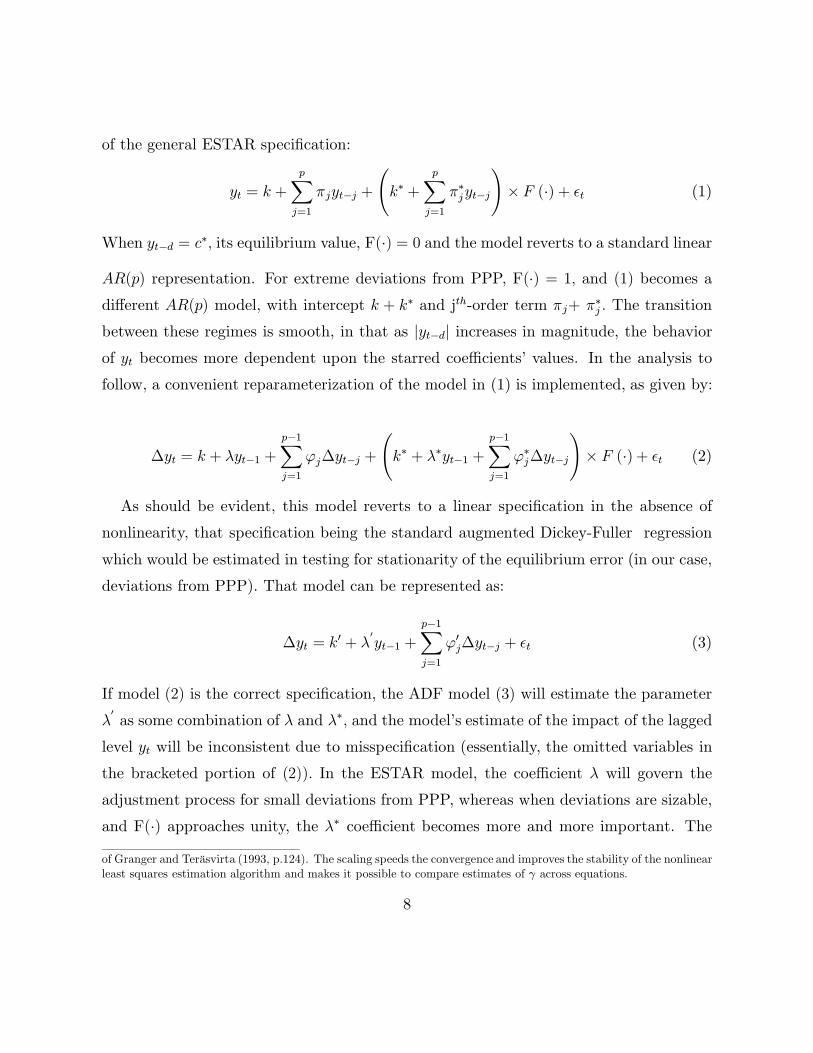
of the general ESTAR speci1cation:
(1)
When its equilibrium value, F and the model reverts to a standard linear
representation. For extreme deviations from PPP, F and becomes a
different model, with intercept and j -order term The transition
between these regimes is smooth, in that as increases in magnitude, the behavior
of becomes more dependent upon the starred coefficientsF values. In the analysis to
follow, a convenient reparameterization of the model in (1) is implemented, as given by:
(2)
As should be evident, this model reverts to a linear speci1cation in the absence of
nonlinearity, that speci1cation being the standard augmented Dickey-Fuller regression
which would be estimated in testing for stationarity of the equilibrium error (in our case,
deviations from PPP). That model can be represented as:
(3)
If model is the correct speci1cation, the ADF model will estimate the parameter
as some combination of and and the modelFs estimate of the impact of the lagged
level will be inconsistent due to misspeci1cation (essentially, the omitted variables in
the bracketed portion of In the ESTAR model, the coefficient will govern the
adjustment process for small deviations from PPP, whereas when deviations are sizable,
and F approaches unity, the coefficient becomes more and more important. The
8
12
12
2.2
∑� �
�
�
� � � � �=1
0 1 22
1 2
( + )
= + + + +
= = 0
( )
Test procedures
t oo
p
j
j t j j t j t d j t j t d t
j j
t
y � � y � y y � y y �
� � j
p,
y
p, d
d
We considered delay length up to 12 months, as it was apparent from the data that longer delay orders than the3 months considered by Michael et al. were preferred.
quantity must be negative to ensure global stability and mean reversion in
the IouterF regime. For small deviations from PPP, however, random-walk behavior is
admissible: that is, may even be positive, implying explosive dynamic behavior, as
long as it does not exceed in absolute value.
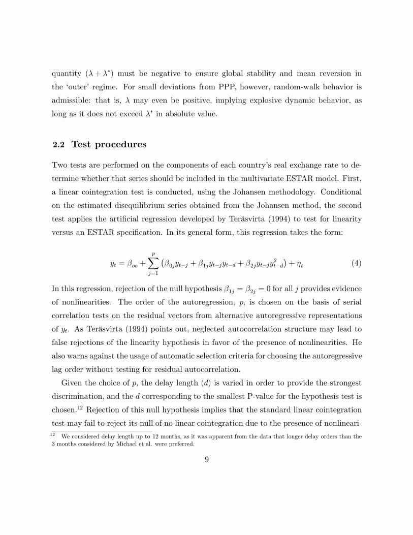
Two tests are performed on the components of each countryFs real exchange rate to de-
termine whether that series should be included in the multivariate ESTAR model. First,
a linear cointegration test is conducted, using the Johansen methodology. Conditional
on the estimated disequilibrium series obtained from the Johansen method, the second
test applies the arti1cial regression developed by Teräsvirta (1994) to test for linearity
versus an ESTAR speci1cation. In its general form, this regression takes the form:
(4)
In this regression, rejection of the null hypothesis for all provides evidence
of nonlinearities. The order of the autoregression, is chosen on the basis of serial
correlation tests on the residual vectors from alternative autoregressive representations
of . As Teräsvirta (1994) points out, neglected autocorrelation structure may lead to
false rejections of the linearity hypothesis in favor of the presence of nonlinearities. He
also warns against the usage of automatic selection criteria for choosing the autoregressive
lag order without testing for residual autocorrelation.
Given the choice of the delay length is varied in order to provide the strongest
discrimination, and the corresponding to the smallest P-value for the hypothesis test is
chosen. Rejection of this null hypothesis implies that the standard linear cointegration
test may fail to reject its null of no linear cointegration due to the presence of nonlineari-
9
�� �
�0 1 2
0
�
�
�
�
2.3
3.1
t
t
t
j j
t
t t t t
t
(2)
= (1 + )
= ( = 1 1)
= 0
= + +
3 Data and Empirical Estimates
y .
y
y c ,
ϕ ϕ , j , ..., p
y
.
.
S � � P � P ε
� S
Parameter restrictions on the ESTAR model
Data
ties in If nonlinearities are present, they imply that the linear cointegrating regression
is misspeci1ed, providing a rationale for 1ndings that fail to support the theory of PPP
as a long-run equilibrium concept.
In this application of the ESTAR model, the nature of as the mean-corrected deviations
from PPP, estimated using the residuals of the cointegrating regression, implies that the
constant terms in may be expected to equal zero. Similarly, the equilibrium value of
in the model, should also equal zero. Given zero values for those three parameters,
further restrictions consistent with this application of ESTAR are and
which imply that when deviations from PPP are large, the
process will be white noise. Conditional on those restrictions, one may test whether
Failure to reject this latter hypothesis would provide support for unit-root behavior
for small deviations from PPP, with mean-reverting adjustment taking place for large
deviations. If all three sets of restrictions may be applied, the ESTAR speci1cation
simpli1es considerably The estimates presented below embody the restrictions which
cannot be rejected by the data.
The PPP hypothesis can be tested by estimating the regression
(5)
where is some constant, is the logarithm of the foreign price of domestic currency at
10
�
13
13
�
�
3.2
1 2 1 2
t t
t
t
t t t( )
(1 1 1)
( = ) ( = = 1)
t P P
t ε t
ε
S , P , P
, ,
� � � �
Tests for cointegration
International Finan-
cial Statistics
All system variables have been tested for the presence of a unit root using the Augmented Dickey-Fuller and
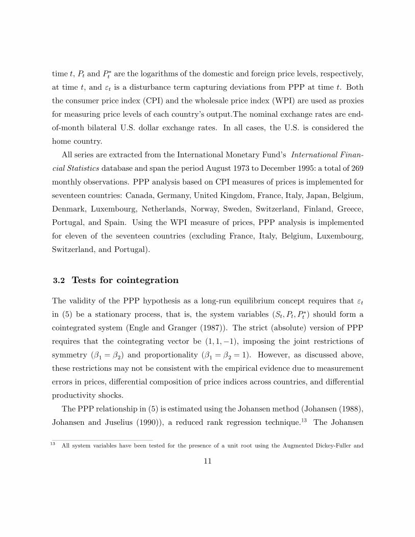
time , and are the logarithms of the domestic and foreign price levels, respectively,
at time , and is a disturbance term capturing deviations from PPP at time . Both
the consumer price index (CPI) and the wholesale price index (WPI) are used as proxies
for measuring price levels of each countryFs output.The nominal exchange rates are end-
of-month bilateral U.S. dollar exchange rates. In all cases, the U.S. is considered the
home country.
All series are extracted from the International Monetary FundFs
database and span the period August 1973 to December 1995: a total of 269
monthly observations. PPP analysis based on CPI measures of prices is implemented for
seventeen countries: Canada, Germany, United Kingdom, France, Italy, Japan, Belgium,
Portugal, and Spain. Using the WPI measure of prices, PPP analysis is implemented
for eleven of the seventeen countries (excluding France, Italy, Belgium, Luxembourg,
Switzerland, and Portugal).
The validity of the PPP hypothesis as a long-run equilibrium concept requires that
in (5) be a stationary process, that is, the system variables should form a
cointegrated system (Engle and Granger (1987)). The strict (absolute) version of PPP
requires that the cointegrating vector be , imposing the joint restrictions of
symmetry and proportionality . However, as discussed above,
these restrictions may not be consistent with the empirical evidence due to measurement
errors in prices, differential composition of price indices across countries, and differential
productivity shocks.
The PPP relationship in (5) is estimated using the Johansen method (Johansen (1988),
Johansen and Juselius (1990)), a reduced rank regression technique. The Johansen
11
′ �
14
14
� , ,= (1 1 1)
Phillips-Perron tests. Consistent with the literature, the null hypothesis of a single unit root cannot be rejected. Toconserve space these results are not reported here but are available upon request.
The multivariate Schwarz information criterion (SIC) was also employed but it generally underestimated the VARlag length, resulting in serially correlated residual vectors from the system equations.
method employs a VAR framework which incorporates both the short- and long-run
dynamics of the system. The lag length of the VAR model for each country is determined
using the multivariate Akaike information criterion (AIC) allowing for a maximum lag
length of twelve. Given the optimal choice of lag length for each country, the estimated
residual vectors from each system equation are tested for serial correlation up to order
twenty-four. If the residual vector from any of the system equations is serially correlated,
the lag length of the VAR is increased until serially uncorrelated residual vectors are
obtained from each system equation.
As Table 1 reports, the Johansen procedure provides evidence of cointegration among
nominal exchange rates and domestic and foreign CPI measures of prices for all coun-
tries but Canada, Germany, Denmark, Norway, Switzerland, and Finland. Weak PPP
is therefore supported for the majority of countries under the current Boat. Absolute
PPP, given by the restriction (symmetry and proportionality), is strongly
rejected for all countries for which a cointegrated system is obtained except Italy.
Using the WPI measures for prices, Table 2 reports that weak PPP is supported for all
countries but Canada, Japan, Sweden, and Greece. The jointly applied proportionality
and symmetry restrictions are strongly rejected in all countries for which exchange rates
and prices form a cointegrated system except Norway, for which the corresponding test
statistic is marginally insigni1cant at the 1ve per cent level. The cointegration evidence
obtained differs for some countries depending upon whether CPI or WPI measures of
prices are used. For Japan, Sweden, and Greece, weak PPP is supported for only CPI
measures of prices while for Germany cointegration evidence between exchange rates and
prices is obtained only in the case of WPI measures.
In summary, the evidence in favor of mean reversion in U.S. dollar-based PPP devi-
ations series is quite strong for the expanded sample period studied here. Furthermore,
12
,
p,
3.3
(4)
15
16 17
15
16
17
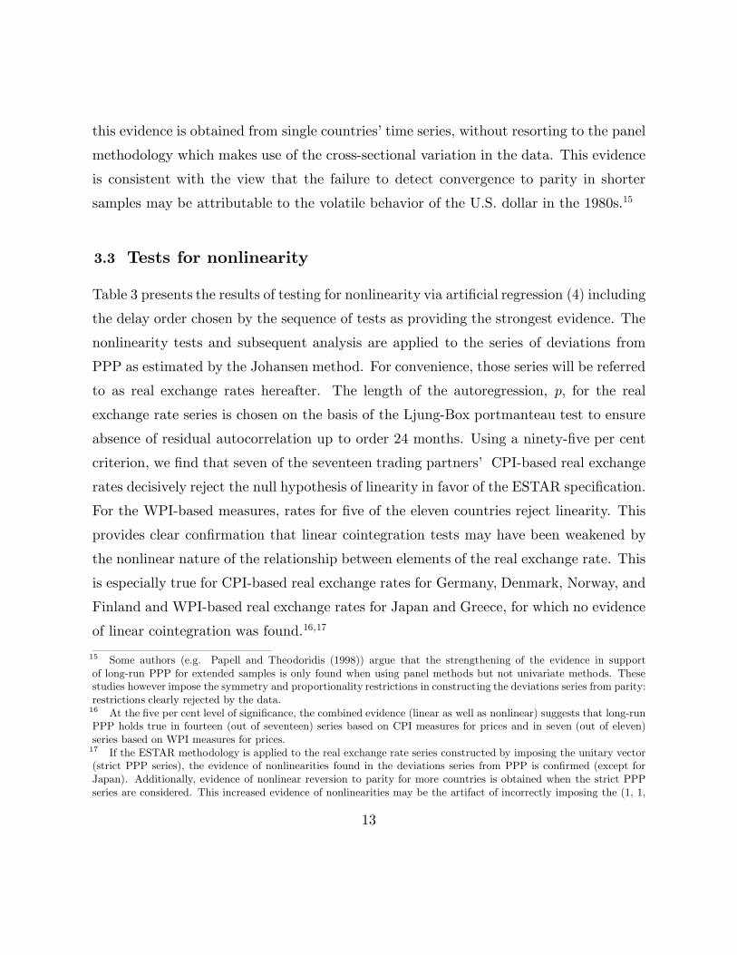
Tests for nonlinearity
Some authors (e.g. Papell and Theodoridis (1998)) argue that the strengthening of the evidence in supportof long-run PPP for extended samples is only found when using panel methods but not univariate methods. Thesestudies however impose the symmetry and proportionality restrictions in constructing the deviations series from parity:restrictions clearly rejected by the data.
At the 1ve per cent level of signi1cance, the combined evidence (linear as well as nonlinear) suggests that long-runPPP holds true in fourteen (out of seventeen) series based on CPI measures for prices and in seven (out of eleven)series based on WPI measures for prices.
If the ESTAR methodology is applied to the real exchange rate series constructed by imposing the unitary vector(strict PPP series), the evidence of nonlinearities found in the deviations series from PPP is con1rmed (except forJapan). Additionally, evidence of nonlinear reversion to parity for more countries is obtained when the strict PPPseries are considered. This increased evidence of nonlinearities may be the artifact of incorrectly imposing the (1, 1,
this evidence is obtained from single countriesF time series, without resorting to the panel
methodology which makes use of the cross-sectional variation in the data. This evidence
is consistent with the view that the failure to detect convergence to parity in shorter
samples may be attributable to the volatile behavior of the U.S. dollar in the 1980s.
Table 3 presents the results of testing for nonlinearity via arti1cial regression including
the delay order chosen by the sequence of tests as providing the strongest evidence. The
nonlinearity tests and subsequent analysis are applied to the series of deviations from
PPP as estimated by the Johansen method. For convenience, those series will be referred
to as real exchange rates hereafter. The length of the autoregression, for the real
exchange rate series is chosen on the basis of the Ljung-Box portmanteau test to ensure
absence of residual autocorrelation up to order 24 months. Using a ninety-1ve per cent
criterion, we 1nd that seven of the seventeen trading partnersF CPI-based real exchange
rates decisively reject the null hypothesis of linearity in favor of the ESTAR speci1cation.
For the WPI-based measures, rates for 1ve of the eleven countries reject linearity. This
provides clear con1rmation that linear cointegration tests may have been weakened by
the nonlinear nature of the relationship between elements of the real exchange rate. This
is especially true for CPI-based real exchange rates for Germany, Denmark, Norway, and
Finland and WPI-based real exchange rates for Japan and Greece, for which no evidence
of linear cointegration was found.
13
3.4
� �
�
�
��
��
0
0
0
0
0
0
0
I
II
j j
III
j
I
II
III
II
t
Estimation of the ESTAR model
: = = = 0
: = (1 + )
= ( = 1 1) 1)
: = 0
= 1 1) = 0
( ) = 0)
ˆ
ˆ 0
ˆ
H k k c
H
ϕ ϕ , j , ..., p , p >
H
�,
ϕ , j , ..., p
F .
�
�
H
H
H >
H
y
-1) vector in the construction of the series, a restriction which is clearly rejected by the data.
The empirical work proceeds with those real exchange rates for which nonlinear be-
havior is signalled by the Table 3 test results at the 1ve per cent level. We determine
the appropriate speci1cation of the model with a series of sequential hypothesis tests.
At the outset, the ESTAR model is estimated, and is tested.
Given a failure to reject those restrictions (which are never rejected by the data), they
are imposed, and the model is reestimated. If the joint hypothesis
(and for those models with cannot be rejected, that
restriction (or set of restrictions) is imposed as well, and the model is again reestimated.
If the hypotheses cannot be rejected, then that restriction is imposed as
well, so that the 1nal model for the series is de1ned by the parameter of the ESTAR
model governing the speed of transition between the two extreme regimes (and possibly
on . The more stringent restriction that implies the presence of
unit-root behavior in the ImiddleF regime (when
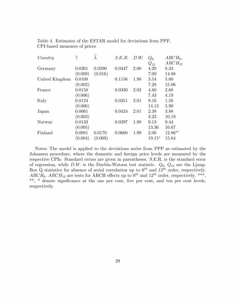
Table 4 presents summary statistics and residual diagnostics of ESTAR models for seven
countriesF CPI-based real exchange rates, while Table 5 presents results from 1ve coun-
triesF WPI-based real exchange rates. The estimates vary widely across countries,
with the speeds of adjustment for some real exchange rates being much higher than oth-
ers. Their values generally support the ESTAR modelFs adequacy, with for most series
being clearly distinguishable from zero. For the CPI-based series, the restrictions
and cannot be rejected for any series, so that the estimated models include two for
which can be rejected: Germany and Finland. For those series, (explosive
behavior in the middle regime) whereas for all other series, cannot be distinguished
from zero (unit-root behavior in the middle regime). For the WPI-based series, may
be rejected for Norway, implying that the process for is not white noise in the outer
14
� 18
�
�
�
�
180
<
�
�
F
F ,
�
H � � F , .�, �,
�
+ 0
ˆ ˆ
( ) = 0)
( ) = 1)
ˆ
: + = 0 (1 263) = 9 168ˆ ˆ
ˆ )
The hypothesis results in an with a marginal signi1cance level of 0.002.However, the evidence for Norway should be interpreted with caution, as none of the crucial coefficients ( and
are individually statistically signi1cant.
regime. However, the stability condition that is satis1ed. For all other
series, cannot be distinguished from zero, and the model is essentially de1ned by .
It must be noted that evidence of nonlinear dynamic adjustment to PPP as well as the
magnitude of the speed-of-adjustment coefficient for a given country can vary, depend-
ing upon the price measure (CPI versus WPI) used in the analysis. Residual diagnostics
indicate that the model generates non-autocorrelated errors at the 1ve per cent level for
every series studied. ARCH effects are present in one of the CPI-based residual series
and in three of the WPI-based residual series. In summary, the ESTAR models appear
to provide a clearly acceptable representation for the adjustment process toward PPP
for both CPI-based and WPI-based series. Models of linear adjustment may be rejected
for the majority of series originally considered, and for many of those series, the ESTAR
model provides a superior alternative.
Based on the empirical estimates, the behavior of deviations from long-run PPP can
be summarized as follows. In the middle regime ( , deviations from parity
persist due to unit-root behavior (explosive behavior for the CPI series for Germany and
Finland and the WPI series for Norway). In the outer regime ( deviations from
parity die out quickly due to their Gwhiteness.H The degree to which deviations from
long-run PPP dissipate is increasing in their magnitude. There is a signi1cant degree of
persistence (before eventual mean reversion occurs) in the outer regime only in the case
of NorwayFs WPI deviations series.
Panels (a) through (g) of Figure 1 graph the estimated transition functions for the CPI-
based deviations series, while panels (a) through (e) of Figure 2 graph these functions for
the WPI-based deviations series. These 1gures con1rm the nonlinearity of the series and
the appropriateness of the exponential transition function. The range of the transition
function values indicates that convergence to long-run PPP is very slow. Additionally, a
comparison of the values of the transition parameter obtained here with those reported
15
�
19
t t[ ] � �
20
3.5
E ω ω .
19
20
1 1
| � |
��
�
� � �
�
� �
1 + 1 + 1
1
01 1
X t t t h t t t h t
X
t t
t t
( ) = [ ] [ ]
1
[ ]
[ ]
= [ ]
GI h, � , ω E X � , ω E X ω
GI X h
� t ω
t
E
E
ω E ω
Generalized impulse response functions
This section was included at the suggestion of an anonymous referee.An alternative strategy of estimating generalized impulse response functions for a nonlinear model involves esti-
mating for each history and then average the obtained sequences over all possible drawings from Givennonlinearities, the impulse response functions derived by these alternative strategies are not expected to be the same.
in Michael et al. (1997) suggests that the persistence of deviations from parity is much
stronger in the post-Bretton Woods era than in the interwar period (the 1920s) or in the
two-century span 1802-1992 included in their study.
To obtain further insights into the dynamic structure of real exchange rates, we perform
impulse response function analysis to evaluate the propagation mechanism of shocks to
the real exchange rate process. Unlike a linear model, impulse response functions for a
nonlinear model are characterized by dependence on initial conditions (history or path
dependence) and the size and sign of the innovation (shock dependence. or asymmetry).
Following Koop et al. (1996), the impulse response function can be expressed as the
difference between two conditional 1rst-moment pro1les:
(6)
where is the generalized impulse response function of a variable , is the fore-
casting horizon, is the perturbation to the process at time , is the conditioning
information set at time (reBecting the history or initial conditions of the variable),
and is the expectations operator. The expression in (6) provides a natural way of
measuring the effect of the shock on the conditional mean of the process.
We produce impulse response functions by estimating corresponding to a repre-
sentative (average) history or initial conditions vector. Setting the conditioning vector to
ensures that the vector of initial conditions G...lies near the center of the
data where the conditional density is most precisely estimatedH (Gallant et al., (1993),
p. 887). The conditional forecasts are simulated realizations obtained by iterating the
16
�21
21
h , , , ...,
.
= 0 1 2 120
1% 2%
h X h X h
X h X h
h
h h
A GI GIGI GI
A h.A A
= (2) 2 (1)(2) (1)
We have also produced estimated IRFs from this strategy (results available on request). The qualitative features oftheir dynamic behavior do not vary signi1cantly from those estimated from the representative history vector, althoughthere are quantitative differences in their time response for several real exchange rate series.
Scale asymmetry for the generalized IRFs can be evaluated by computing a serieswhere and are the generalized IRFs for a +2% and +1% innovation, respectively. For a linearIRF (such as that derived from a standard VAR model) the series would be zero at all The degree to which
differs from zero indicates the magnitude of nonlinear effects in the estimated ESTAR models. Graphs of theseries (available upon request) indicate that for most of the 12 models considered, sizable deviations from zero areapparent in these measures of scale asymmetry.
time series model, randomly drawing with replacement from the estimated residuals of
the model, and then averaging over the number of random draws (see Koop et al.(1996)
for a detailed description of this methodology). For our real exchange rate series, we
derive impulse response functions by setting months and averaging the
conditional forecast for each forecasting horizon over 5,000 draws.
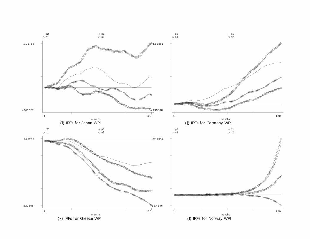
The panels in Figure 3 display the cumulative impulse response functions for the levels
of CPI-based and WPI-based real exchange rate series corresponding to perturbations in
the vector of initial conditions by +/- and +/- . The particular sort of nonlinearity
assumed in the use of the ESTAR framework is scale asymmetry: a larger deviation from
PPP should have a more than proportional effect on the modelFs dynamic path relative to
a smaller innovation. In interpreting the dynamic response sequences of the deviations
series from PPP, it must be kept in mind that the chosen AR and delay-parameter
structures for our ESTAR series (see Table 3) are generally of high order, giving rise to
rather complex nonlinear dynamic behavior
An inspection of the generalized impulse response functions reveals the presence of
signi1cant nonlinearities in the dynamic response of real exchange rates to innovations.
The following general observations are in order:
i) Shocks of differing magnitude (e.g. 1% versus 2%) have disproportionate effects.
The dynamic structure of the series is characterized by scale asymmetry (asymmetry
based on the size of the shock). As mentioned earlier, such behavior is a feature of the
ESTAR model.
ii) Positive and negative shocks of the same magnitude appear to have differential
dynamic effects (in absolute value terms), thus suggesting sign asymmetry (asymmetry
17
�ˆ ˆ
22
22
4 Conclusions
This asymmetry is apparent if the absolute magnitude of impulse responses to a positive and negative shock ofequal magnitude are compared.
based on the sign of the shock). The observed sign asymmetry may be indicative of
more complex nonlinear dynamics than that captured by the estimated ESTAR models.
iii) In most cases, innovations to the process appear to die out, suggesting mean
reversion. However, the speed of dissipation and degree of persistence vary considerably
across series and shocks to the series.
The WPI-based real exchange rate series for Norway exhibits long-run explosive dy-
namics. This arises since, based on the and coefficient estimates reported in Table 5,
this series is characterized by explosive behavior in the middle regime and near-unit-root
behavior in the outer regime. Such behavior leads to signi1cant instability in the dynamic
structure of the series, as exhibited by the estimated impulse response sequences.
Although the combined evidence from the generalized impulse response functions may
be difficult to interpret and generalize, it is clearly indicative of the presence of severe
nonlinearities in the dynamic structure of the real exchange rate series. These nonlinear-
ities call into question the results of many studies which have been generated conditional
on the adequacy of a linear dynamic structure for real exchange rate series.
Earlier studies have had difficulty detecting convergence to long-run PPP in the post-
Bretton Woods era, thus suggesting the absence of a link between nominal exchange rates
and prices in open economies. Perhaps the well-known weaknesses of unit-root tests in
temporally limited samples may account for the prevalence of unit-root 1ndings and the
seeming rejection of long-run PPP. Recently, the panel unit-root literature has provided
one avenue by which data from this limited temporal span may be used to detect conver-
gence. In contrast, our 1ndings demonstrate that the evidence in favor of PPP markedly
strengthens when JohansenFs cointegration framework is applied to this expanded sample
18
Acknowledgements
period from the current Boat, without resort to the cross-sectional variation in the data
upon which the panel framework relies. Moreover, by allowing for the presence of non-
linearities in the dynamic adjustment to deviations from PPP in an ESTAR framework,
our study provides additional evidence of a mean-reverting dynamic process for sizable
deviations from PPP in several countriesF series, with an equilibrium tendency varying
with the magnitude of disequilibrium. Evidence from generalized impulse response func-
tions also supports the presence of nonlinearities. This evidence of nonlinear adjustment
to parity is in contrast to the negative evidence obtained by OFConnell (1998b) for panels
of real exchange rates in a TAR framework.
Although the unit-root hypothesis may be rejected for a number of the PPP devi-
ations series, a shock to these series dies out very slowly. Future research may focus
on the factors that distinguish those countries whose deviations from long-run PPP are
characterized by nonlinear behavior, as well as those related to this unusually slow speed
of adjustment. The high volatility of the nominal exchange rate for the U.S. dollar in
the 1980s may provide an explanation for the latter.
We are grateful to Peter Pedroni and Nikolay Gospodinov for their useful suggestions,
and to participants in the CEFESF98 conference for their comments on an earlier draft.
Two anonymous reviewers of this journal provided a very useful critique of the paper.
The standard disclaimer applies.
19
References
Balke, N., Fomby, T., 1997. Threshold cointegration. International Economic Review
38 (3), 627-645.
Cheung, Y.-M., Lai, K., 1993. Long-run purchasing power parity during the recent
Boat. Journal of International Economics 34, 181-192.
Coleman, A.M., 1995. Arbitrage, storage and the GLaw of one priceH: New theory
for the time series analysis of an old problem. Unpublished working paper, Princeton
University, Princeton NJ.
Corbae, D., Ouliaris, S., 1988. Cointegration and tests of purchasing power parity.
Review of Economics and Statistics 70, 508-511.
Diebold, F. X., Husted, S., Rush, M., 1991. Real exchange rates under the gold
standard. Journal of Political Economy 99, 1252-1271.
Dumas, B., 1992. Dynamic equilibrium and the real exchange rate in a spatially
separated world. Review of Financial Studies 5 (2), 153-180.
Edison, H. J., Fisher, E.O., 1991. A long-run view of the European monetary system.
Journal of International Money and Finance 10, 53-70.
Engel, C., Hendrickson, M., Rogers, J., 1997. Intra-national, intra-continental and
intra-planetary PPP. National Bureau of Economic Research, Cambridge MA. Working
Paper 6069.
Engle, R. F., Granger, C.W.J., 1987. Co-integration and error correction: represen-
tation, estimation, and testing. Econometrica 55, 251-276.
Fisher, E., Park, J., 1991. Testing purchasing power parity under the null hypothesis
of cointegration. Economic Journal 101, 1476-1484.
Frankel, J. A., Rose, A., 1996. Mean reversion within and between countries: A panel
project on purchasing power parity. Journal of International Economics 40, 209-224.
Froot, K. A., Rogoff, K., 1995. Perspectives on PPP and long-run real exchange rates.
In: Grossman, G., Rogoff, K. (Eds.), Handbook of International Economics. North-
Notes: The system variables are where is the logarithm of the foreign price of domestic currency at timeand and are the logarithms of the domestic and foreign levels of the consumer price index (CPI), respectively, at timeThe value indicates the order of the vector error correction model (VECM) estimated for each country. The Johansen
25
′′
02
�
�: = (1 1 1)
p r
p r
� S.H � , , �
trace test statistics have been modi=ed to account for =nite-sample bias, following the correction suggested by Reinsel andAhn (1992) and Reimers (1992). The asymptotic critical values (without drift in the data generating process), obtainedfrom Osterwald-Lenum (1992), are presented in the following table, in which is the number of system variables and isthe cointegration rank:
The cointegrating vector has been normalized with respect to the nominal exchange rate variable The LR teststatistic for is distributed under the null hypothesis with two degrees of freedom (marginal signi=cancelevels are given in parentheses). ***, **, * indicate signi=cance at the one per cent, =ve per cent, and ten per cent levels,respectively.
26
� � �0 0 0 0
t t t t
t t
Country : 2 : 1 : = 0 : = (1 1 1)
( )
′ ′
� ���� ��
� ���� ���
�
�
� �
��
k H r H r H r � H � , ,
S , P , P , St P P
t. k
Table 2. Johansen Cointegration Results for the PPP Hypothesis, WPI-based Measures
Notes: The system variables are where is the logarithm of the foreign price of domestic currency at timeand and are the logarithms of the domestic and foreign levels of the wholesale price index (WPI), respectively,
at time The value indicates the order of the vector error correction model (VECM) estimated for each country. TheJohansen trace test statistics have been modi=ed to account for =nite-sample bias, following the correction suggested byReinsel and Ahn (1992) and Reimers (1992). See notes in Table 1 for additional explanation of the table.
27
� { }t d 1 12
d d
dy , p
Country Optimal p P-value Optimal p P-value
Table 3. Tests for linearity of the cointegrating regression
Notes: The tests are performed on the deviations from PPP as estimated by theJohansen method. The optimal is chosen by minimizing the P-value of the linearitytest for the delay parameter over the range given the autoregressive orderwhich was chosen on the basis of serial correlation tests.
28
���
Country ,
th th
th th
6 6
12 12
6 12
6 12
� S.E.R. D.W. Q ARCH ,Q ARCH
D.W. Q , Q
ARCH , ARCH
Table 4. Estimates of the ESTAR model for deviations from PPP,CPI-based measures of prices
Finland 0.0081 0.0170 0.0660 1.99 2.00 12.86(0.004) (0.009) 19.15 15.84
Notes: The model is applied to the deviations series from PPP as estimated by theJohansen procedure, where the domestic and foreign price levels are measured by therespective CPIs. Standard errors are given in parentheses. S.E.R. is the standard errorof regression, while is the Durbin-Watson test statistic. are the Ljung-Box Q statistics for absence of serial correlation up to 6 and 12 order, respectively.
are tests for ARCH effects up to 6 and 12 order, respectively. ***,**, * denote signi1cance at the one per cent, 1ve per cent, and ten per cent levels,respectively.
29
, 6 6
12 12
Country�
��
� ���
���
� S.E.R. D.W. Q ARCH ,Q ARCH
Table 5. Estimates of the ESTAR model for deviations from PPP,WPI-based measures of prices