Nonlinear Control and Servo systems

Lecture 1

Giacomo Como, 2013

Dept. of Automatic ControlLTH, Lund University

Overview Lecture 1

• Practical information• Course contents• Nonlinear control phenomena• Nonlinear differential equations

Course Goal

To provide students with a solid theoretical foundation ofnonlinear control systems combined with a good engineeringability

You should after the course be able to

recognize common nonlinear control problems, use some powerful analysis methods, and use some practical design methods.

Today’s Goal

Recognize some common nonlinear phenomena Transform differential equations to autonomous form,

first-order form, and feedback form. Describe saturation, dead-zone, relay with hysteresis,

backlash Calculate equilibrium points

Course Material

Textbook Glad and Ljung, Reglerteori, flervariabla och olinjära

metoder, 2003, Studentlitteratur,ISBN 9-14-403003-7 or theEnglish translation Control Theory, 2000, Taylor & FrancisLtd, ISBN 0-74-840878-9. The course covers Chapters11-16,18. (MPC and optimal control not covered in theother alternative textbooks.)

H. Khalil, Nonlinear Systems (3rd ed.), 2002, Prentice Hall,ISBN 0-13-122740-8. A good, but a bit more advancedbook.

Course Material, cont.

Handouts (Lecture notes + extra material)

Exercises (can be download from the course home page)

Lab PMs 1, 2 and 3

Home pagehttp://www.control.lth.se/course/FRTN05/

Matlab/Simulink other simulation softwaresee home page

Lectures and labs

The lectures (30 hours) are given as follows:

Mon 13–15, M:E Jan 21 – Feb 25Wed 8–10, M:E Jan 23 – Feb 27Thu 10-12 M:E Jan 24Mon 13-15 M:D Mar 4

The lectures are given in English.

———————

The three laboratory experiments are mandatory.

Sign-up lists are posted on the web at least one week beforethe first laboratory experiment. The lists close one day beforethe first session.

The Laboratory PMs are available at the course homepage.

Before the lab sessions some home assignments have to bedone. No reports after the labs.

Exercise sessions and TAs

The exercises (28 hours) are offered twice a week;

Tue 15-17 Wed 15-17

NOTE: The exercises are held in either ordinary lecture rooms or thedepartment laboratory on the bottom floor in the south end of theMechanical Engineering building, see schedule on home page.

Anders Mannesson Olof Sörnmo,

The Course

14 lectures

14 exercises

3 laboratories

5 hour exam: March 13, 2013, 8:00-13:00 .Open-book exam: Lecture notes but no old exams orexercises allowed. Next exam on April ??, 2013

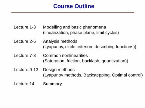
Course Outline

Lecture 1-3 Modelling and basic phenomena(linearization, phase plane, limit cycles)

Lecture 2-6 Analysis methods(Lyapunov, circle criterion, describing functions))

Lecture 7-8 Common nonlinearities(Saturation, friction, backlash, quantization))

Lecture 9-13 Design methods(Lyapunov methods, Backstepping, Optimal control)

Lecture 14 Summary

Todays lecture

Common nonlinear phenomena

Input-dependent stability Stable periodic solutions Jump resonances and subresonances

Nonlinear model structures

Common nonlinear components State equations Feedback representation

Linear Systems

Su y = S(u)

Definitions: The system S is linear if

S(αu) = α S(u), scaling

S(u1 + u2) = S(u1) + S(u2), superposition

A system is time-invariant if delaying the input results in adelayed output:

y(t− τ ) = S(u(t− τ ))

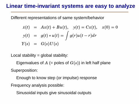
Linear time-invariant systems are easy to analyze

Different representations of same system/behavior

x(t) = Ax(t) + Bu(t), y(t) = Cx(t), x(0) = 0

y(t) = (t) ⋆ u(t) =∫

(r)u(t− r)dr

Y(s) = G(s)U(s)

Local stability = global stability:

Eigenvalues of A (= poles of G(s)) in left half plane

Superposition:

Enough to know step (or impulse) response

Frequency analysis possible:

Sinusoidal inputs give sinusoidal outputs

Linear models are not always enough

Example: Ball and beam

x

m

m sin(φ)

φ

Linear model (acceleration along beam) :Combine F = m ⋅ a = md2x

dt2and F = m sin(φ):

x(t) = φ(t)

Linear models are not enough

x = position (m)

φ = angle (rad)

= 9.81 (m/s2)

Can the ball move 0.1 meter in 0.1 seconds?

Solving d2

dt2x = φ0 gives

x(t) = t2

2φ0

φ0 = 2 ∗ 0.1

0.12 ∗ ≥ 2 rad

Clearly outside linear region!

Contact problem, friction, centripetal force, saturation

How fast can it be done? (Optimal control)

2 minute exercise: Find a simple system x = f (x,u) that isstable for a small input step but unstable for large input steps.

Stability Can Depend on Amplitude

?+ 1s

1(s+1)2

Motor Valve Process

−1

r y

Valve characteristic f (x) =???Step changes of amplitude, r = 0.2, r = 1.68, and r = 1.72

Stability Can Depend on Amplitude

+ 1s

1(s+1)2

Motor Valve Process

−1

r y

Valve characteristic f (x) = x2

Step changes of amplitude, r = 0.2, r = 1.68, and r = 1.72

Step Responses

0 5 10 15 20 25 300

0.2

0.4

Time t

Out

put y

0 5 10 15 20 25 300

2

4

Time t

Out

put y

0 5 10 15 20 25 300

5

10

Time t

Out

put y

r = 0.2

r = 1.68

r = 1.72

Stability depends on amplitude!

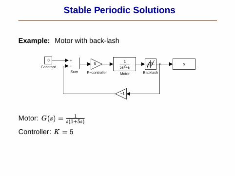
Stable Periodic Solutions

Example: Motor with back-lash

y

Sum

5

P−controller

1

5s +s2

Motor

0

Constant

Backlash

−1

Motor: G(s) = 1s(1+5s)

Controller: K = 5

Stable Periodic Solutions

Output for different initial conditions:

0 10 20 30 40 50−0.5

0

0.5

Time tO

utpu

t y

0 10 20 30 40 50−0.5

0

0.5

Time t

Out

put y

0 10 20 30 40 50−0.5

0

0.5

Time t

Out

put y

Frequency and amplitude independent of initial conditions!

Several systems use the existence of such a phenomenon

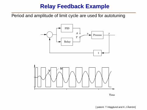
Relay Feedback Example

Period and amplitude of limit cycle are used for autotuning

Σ Process

PID

Relay

A

T

u y

− 1

0 5 1 0

− 1

0

1

Time

uy

[ patent: T Hägglund and K J Åström]

Jump Resonances

y

SumSine Wave

Saturation

20

5s +s2

Motor

−1

Response for sinusoidal depends on initial condition

Problem when doing frequency response measurement

Jump Resonances

u = 0.5 sin(1.3t), saturation level =1.0

Two different initial conditions

0 10 20 30 40 50−6

−4

−2

0

2

4

6

Time t

Out

put y

give two different amplifications for same sinusoid!

Jump Resonances

Measured frequency response (many-valued)

10−1

100

101

10−3

10−2

10−1

100

101

Mag

nitu

de

Frequency [rad/s]

linearsaturated

saturated

New Frequencies

Example: Sinusoidal input, saturation level 1

a sin t y

Saturation

100

10−2

100

Frequency (Hz)

Am

plitu

de y

0 1 2 3 4 5−2

−1

0

1

2

Time t

100

10−2

100

Frequency (Hz)

Am

plitu

de y

0 1 2 3 4 5−2

−1

0

1

2

Time t

a = 1

a = 2a = 2a = 2a = 2

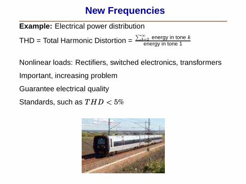
New Frequencies

Example: Electrical power distribution

THD = Total Harmonic Distortion =∑∞k=2 energy in tone kenergy in tone 1

Nonlinear loads: Rectifiers, switched electronics, transformers

Important, increasing problem

Guarantee electrical quality

Standards, such as THD < 5%

New Frequencies

Example: Mobile telephone

Effective amplifiers work in nonlinear region

Introduces spectrum leakage

Channels close to each other

Trade-off between effectivity and linearity

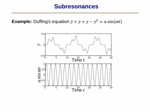
Subresonances

Example: Duffing’s equation y+ y+ y− y3 = a sin(ω t)

0 5 10 15 20 25 30−0.5

0

0.5

0 5 10 15 20 25 30−1

−0.5

0

0.5

1

Time t

Time t

yasin

ωt

When is Nonlinear Theory Needed?

Hard to know when - Try simple things first! Regulator problem versus servo problem Change of working conditions (production on demand,

short batches, many startups) Mode switches Nonlinear components

How to detect? Make step responses, Bode plots

Step up/step down Vary amplitude Sweep frequency up/frequency down

Some Nonlinearities

Static – dynamic

Sign

Saturation

Relay

eu

MathFunction

Look−UpTable

Dead Zone

Coulomb &Viscous Friction

Backlash

|u|

Abs

2 minute exercise

Construct a model for a “rate limiter” using some of the previousnonlinear blocks.

Nonlinear Differential Equations

Problems

No analytic solutions Existence? Uniqueness? etc

Existence Problems

Example: The differential equation

dx

dt= x2, x(0) = x0

has solution

x(t) = x0

1− x0t, 0 ≤ t < 1

x0

Finite escape time

t f =1

x0

Finite Escape Time

0 1 2 3 4 50

0.5

1

1.5

2

2.5

3

3.5

4

4.5

5

Time t

x(t

)

Finite escape time of dx/dt = x2

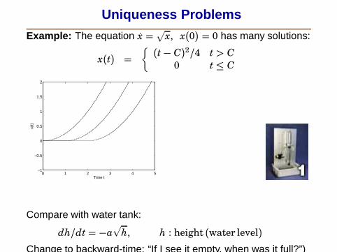
Uniqueness Problems

Example: The equation x = √x, x(0) = 0 has many solutions:

x(t) =

(t− C)2/4 t > C0 t ≤ C

0 1 2 3 4 5−1

−0.5

0

0.5

1

1.5

2

Time t

x(t)

Compare with water tank:

dh/dt = −a√h, h : height (water level)

Change to backward-time: “If I see it empty, when was it full?”)

Existence and Uniqueness

TheoremLet ΩR denote the ball

ΩR = z; qz− aq ≤ R

If f is Lipschitz-continuous:

q f (z) − f (y)q ≤ Kqz− yq, for all z, y∈ Ω

then x(t) = f (x(t)), x(0) = a has a unique solution in

0 ≤ t < R/CR,

where CR = maxΩR q f (x)q

State-Space Models

State vector x Input vector u Output vector y

general: f (x,u, y, x, u, y, . . .) = 0explicit: x = f (x,u), y = h(x)

affine in u: x = f (x) + (x)u, y= h(x)linear time-invariant: x = Ax + Bu, y= Cx

Transformation to Autonomous System

Nonautonomous:x = f (x, t)

Always possible to transform to autonomous system

Introduce xn+1 = time

x = f (x, xn+1)xn+1 = 1

Transformation to First-Order System

Assume dky

dtkhighest derivative of y

Introduce x =[

y dydt. . . dk−1y

dtk−1

]T

Example : Pendulum

MRθ + kθ +MR sinθ = 0

x =[

θ θ]T

gives

x1 = x2

x2 = − k

MRx2 −

Rsin x1

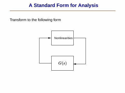
A Standard Form for Analysis

Transform to the following form

G(s)

Nonlinearities

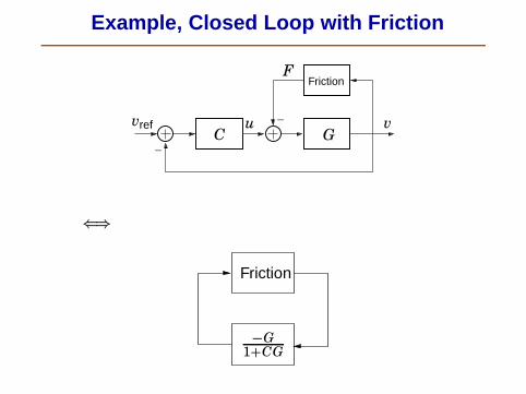
Example, Closed Loop with Friction

_

_GC

Friction

vref u

F

v

Z[

−G1+CG

Friction

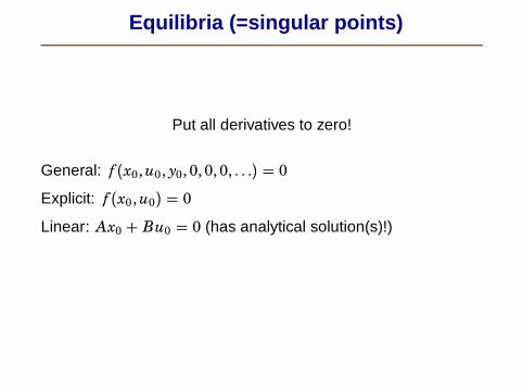
Equilibria (=singular points)

Put all derivatives to zero!

General: f (x0,u0, y0, 0, 0, 0, . . .) = 0Explicit: f (x0,u0) = 0Linear: Ax0 + Bu0 = 0 (has analytical solution(s)!)

Multiple Equilibria

Example: Pendulum

MRθ + kθ +MR sinθ = 0

Equilibria given by θ = θ = 0 =[ sinθ = 0 =[ θ = nπAlternatively,

x1 = x2

x2 = − k

MRx2 −

Rsin x1

gives x2 = 0, sin(x1) = 0, etc

Next Lecture

Linearization Stability definitions Simulation in Matlab