46
Nonlinear Data Assimilation and Particle Filters Peter Jan van Leeuwen
| Date post: | 29-Dec-2015 |
| Category: |
Documents |
| Upload: | barnard-manning |
| View: | 217 times |
| Download: | 3 times |
Nonlinear Data Assimilationand Particle Filters
Peter Jan van Leeuwen

Data Assimilation Ingredients
• Prior knowledge, the Stochastic model:
• Observations:
• Relation between the two:
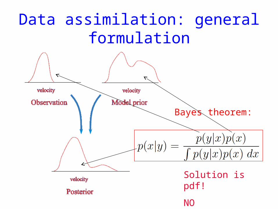
Data assimilation: general formulation
Solution is pdf!
NO INVERSION !!!
Bayes theorem:
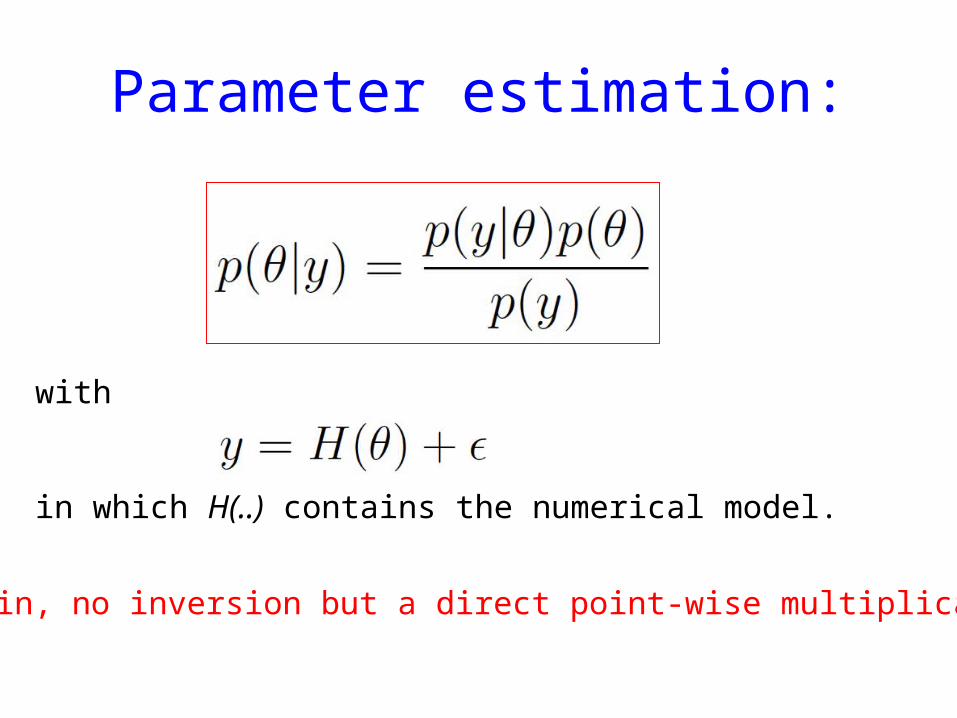
Parameter estimation:
with
in which H(..) contains the numerical model.
Again, no inversion but a direct point-wise multiplication.

Propagation of pdf in time: Kolmogorov’s equation
Model equation:
Pdf evolution: Kolmogorov’s equation(Fokker-Planck equation)
advection diffusion
Too expensive !!!
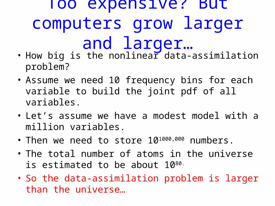
Too expensive? But computers grow larger and larger…
• How big is the nonlinear data-assimilation problem? • Assume we need 10 frequency bins for each variable
to build the joint pdf of all variables.• Let’s assume we have a modest model with a million
variables.• Then we need to store 101000,000 numbers.• The total number of atoms in the universe is
estimated to be about 1080.
• So the data-assimilation problem is larger than the universe…
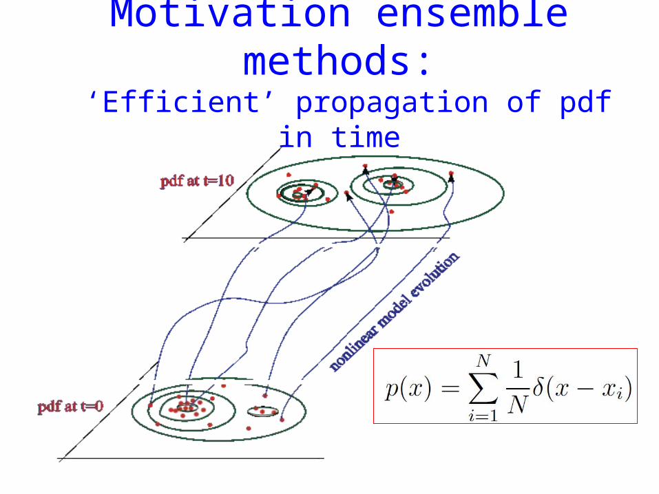
Motivation ensemble methods: ‘Efficient’ propagation of pdf in time
How is DA used today in geosciences?Present-day data-assimilation systems are based on
linearizations and state covariances are essential.
4DVar, Representer method (PSAS):- Gaussian pdf’s , solves for posterior mode, needs error covariance of initial state (B matrix), ‘no’ posterior error covariances
(Ensemble) Kalman filter: - assumes Gaussian pdf’s for the state, approximates posterior mean and covariance, doesn’t minimize anything in nonlinear systems, needs inflation and localisation
Combinations of these: hybrid methods (!!!)
Non-linear Data Assimilation
• Metropolis-Hastings Start from one sample, generate a new one and decide on acceptance (better, or by chance), etc. Slow convergence, but new smarter algorithms are being devised.
• Langevin sampling Idem, but always accept, each sample expensive. Slow convergence, but smarter algorithms are being devised.
• Hybrid Monte-Carlo idem, but almost always accept, each sample expensive, faster convergence
Non-linear Data Assimilation
• Particle Filters/Smoothers Generate samples in parallel sequential over time and weight them according how good they are. Importance sampling. Can be made very efficient.
• Combinations of MH and PF Expensive but good for e.g. parameter estimation.
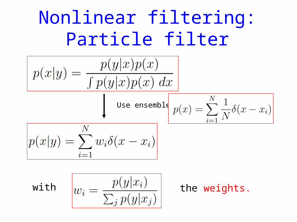
Nonlinear filtering: Particle filter
Use ensemble
with the weights.
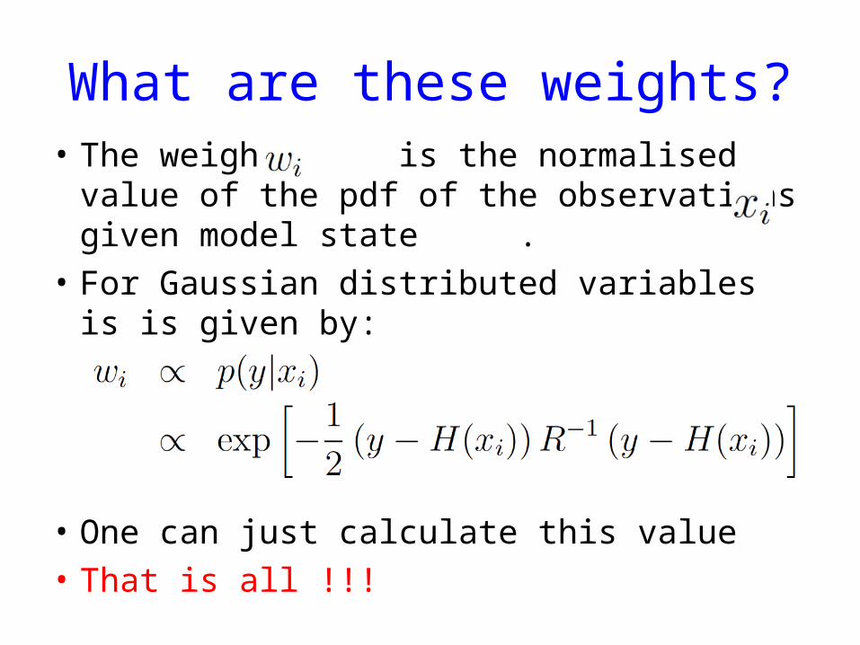
What are these weights?• The weight is the normalised value of the
pdf of the observations given model state .• For Gaussian distributed variables is is given
by:
• One can just calculate this value• That is all !!!
No explicit need for state covariances
• 3DVar and 4DVar need a good error covariance of the prior state estimate: complicated
• The performance of Ensemble Kalman filters relies on the quality of the sample covariance, forcing artificial inflation and localisation.
• Particle filter doesn’t have this problem, but…
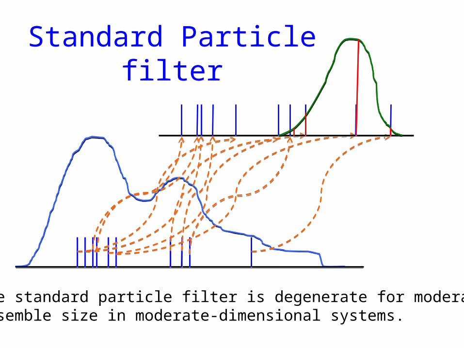
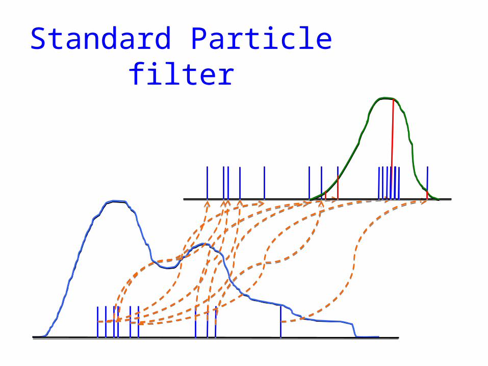
Standard Particle filter
The standard particle filter is degenerate for moderate ensemble size in moderate-dimensional systems.
Particle Filter degeneracy: resampling
• With each new set of observations the old weights are multiplied with the new weights.
• Very soon only one particle has all the weight…
• Solution: Resampling: duplicate high-weight particles and abandon low-weight particles
Standard Particle filter
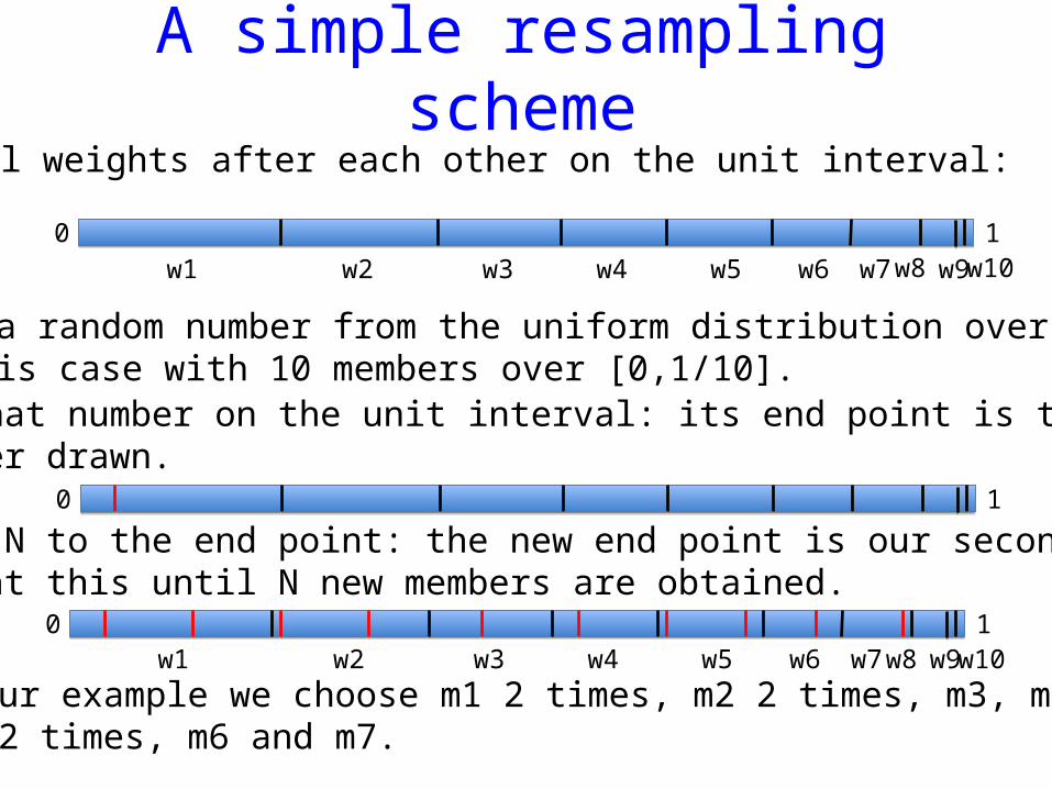
A simple resampling scheme1. Put all weights after each other on the unit interval:
0 1w1 w2 w3 w4 w5 w6 w7w8 w9w10
2. Draw a random number from the uniform distribution over [0,1/N], in this case with 10 members over [0,1/10].3. Put that number on the unit interval: its end point is the first member drawn.
4. Add 1/N to the end point: the new end point is our second member. Repeat this until N new members are obtained.0 1
w1 w2 w3 w4 w5 w6 w7w8 w9w10
5. In our example we choose m1 2 times, m2 2 times, m3, m4, m5 2 times, m6 and m7.
0 1
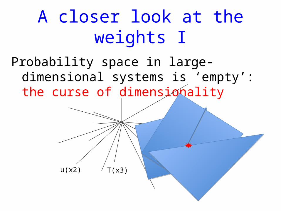
A closer look at the weights I
Probability space in large-dimensional systems is ‘empty’: the curse of dimensionality
u(x1)
u(x2) T(x3)
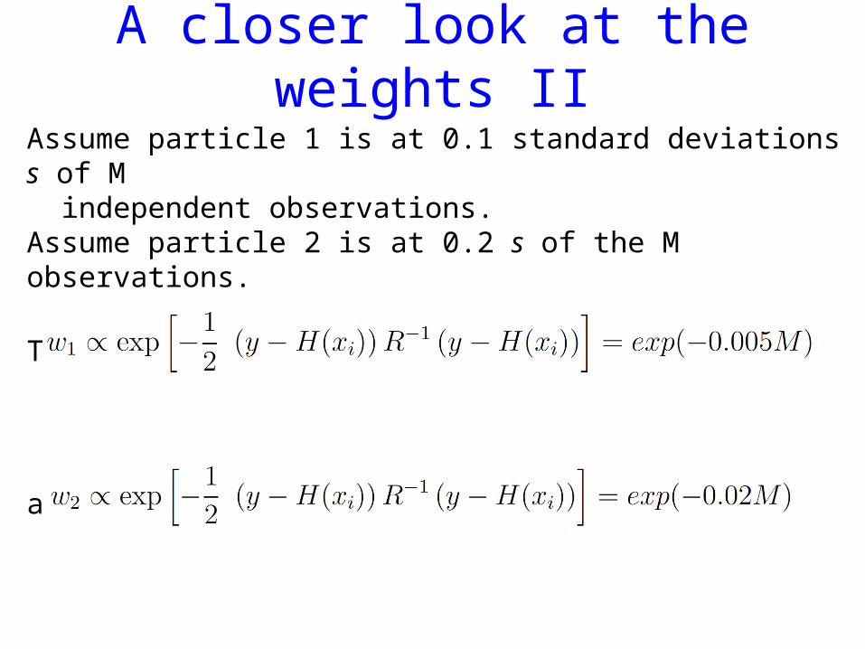
A closer look at the weights IIAssume particle 1 is at 0.1 standard deviations s of M independent observations.Assume particle 2 is at 0.2 s of the M observations.
The weight of particle 1 will be
and particle 2 gives
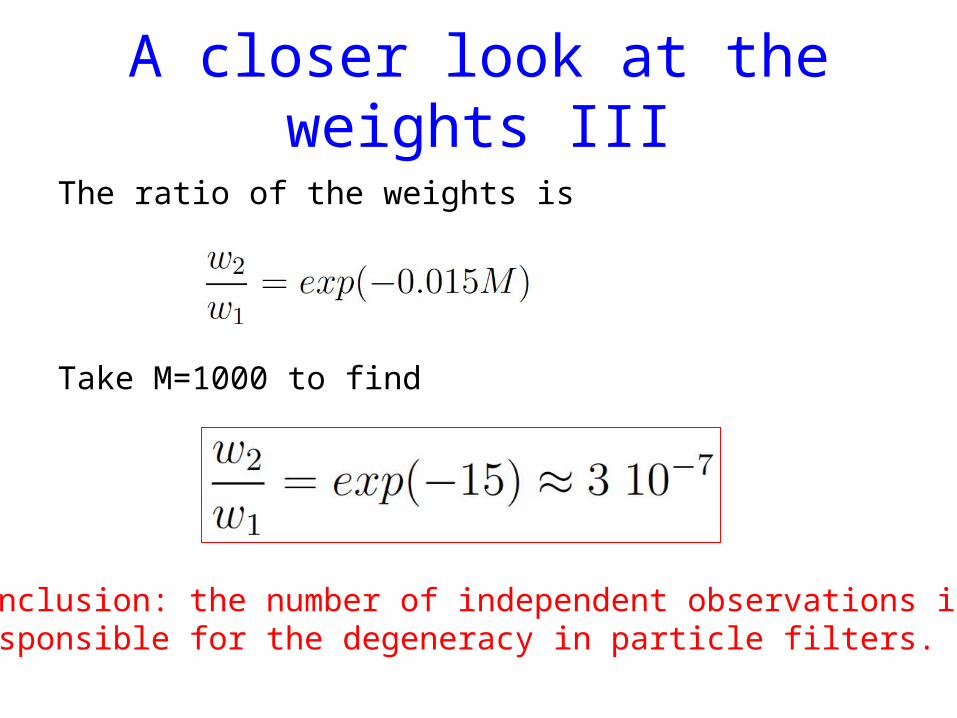
A closer look at the weights III
The ratio of the weights is
Take M=1000 to find
Conclusion: the number of independent observations isresponsible for the degeneracy in particle filters.
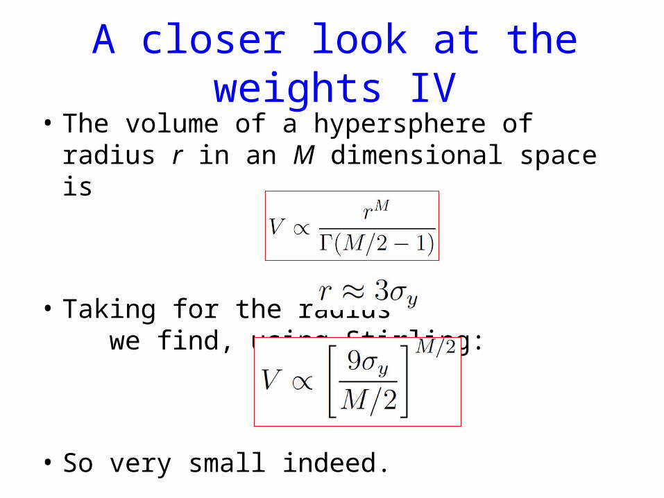
A closer look at the weights IV• The volume of a hypersphere of radius r in an
M dimensional space is
• Taking for the radius we find, using Stirling:
• So very small indeed.
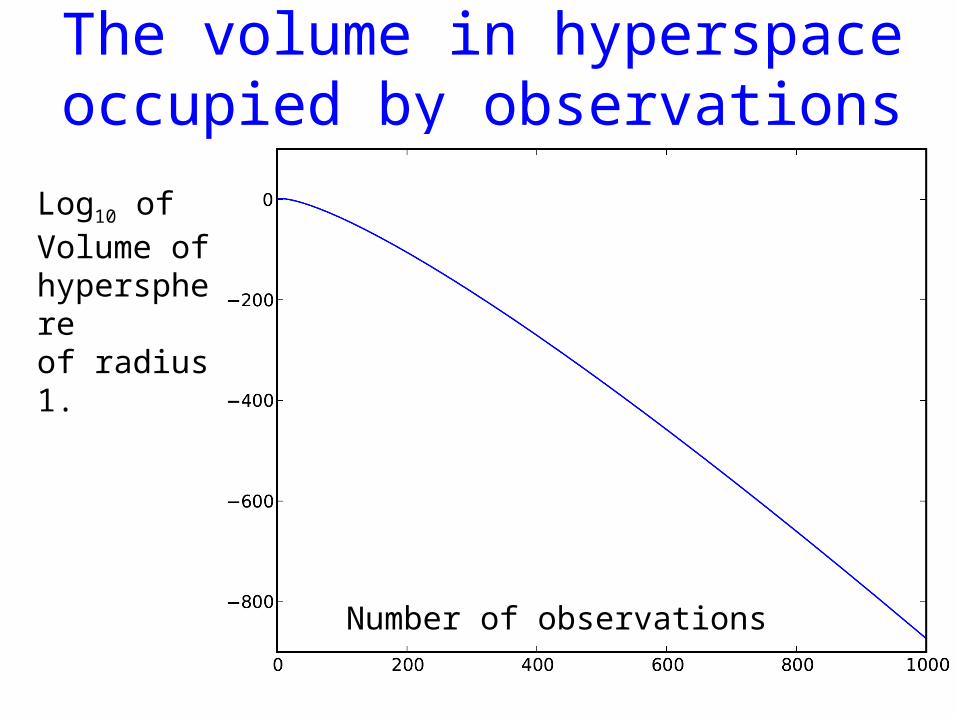
The volume in hyperspace occupied by observations
Number of observations
Log10 of Volume of hypersphereof radius 1.
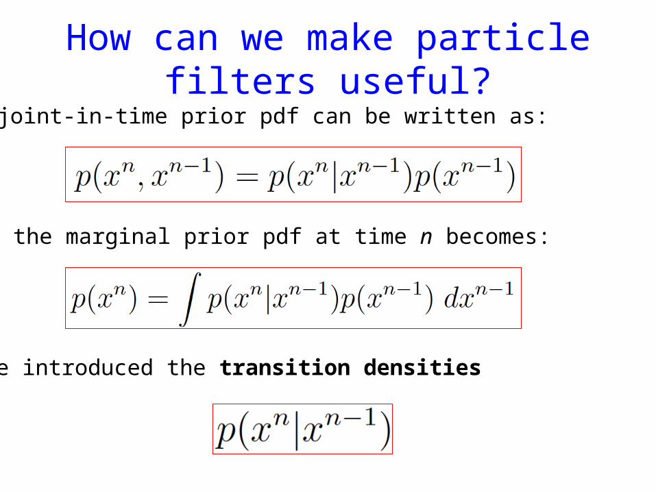
How can we make particle filters useful?
We introduced the transition densities
The joint-in-time prior pdf can be written as:
So the marginal prior pdf at time n becomes:
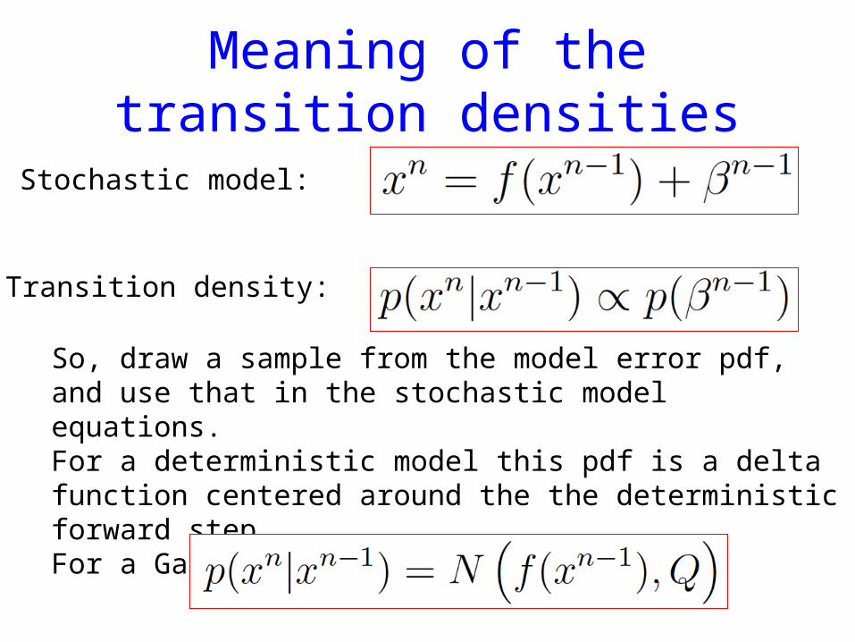
Meaning of the transition densities
So, draw a sample from the model error pdf, and use that in the stochastic model equations.For a deterministic model this pdf is a delta function centered around the the deterministic forward step.For a Gaussian model error we find:
Stochastic model:
Transition density:
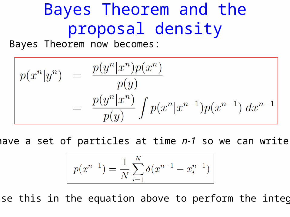
Bayes Theorem and the proposal densityBayes Theorem now becomes:
We have a set of particles at time n-1 so we can write
and use this in the equation above to perform the integral:
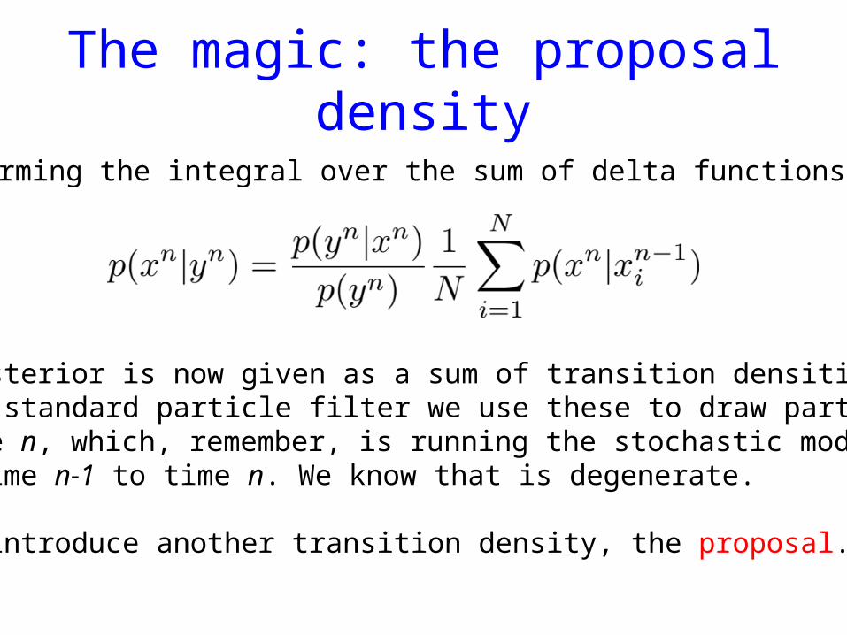
The magic: the proposal density
The posterior is now given as a sum of transition densities.In the standard particle filter we use these to draw particles at time n, which, remember, is running the stochastic modelfrom time n-1 to time n. We know that is degenerate.
So we introduce another transition density, the proposal.
Performing the integral over the sum of delta functions gives:

The proposal transition density
Multiply numerator and denominator with a proposal density q:
Note that 1) the proposal depends on the future observation, and2) the proposal depends on all previous particles, not just one.
1)Ensures that the particles end up close to the observations because they know where the observations are.2) Allows for an equal-weight filter, as the performance boundssuggested by Snyder, Bickel, and Bengtsson do not apply.
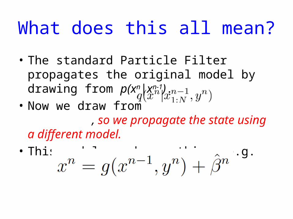
What does this all mean?
• The standard Particle Filter propagates the original model by drawing from p(xn|xn-1).
• Now we draw from , so we propagate the state using a different model.
• This model can be anything, e.g.
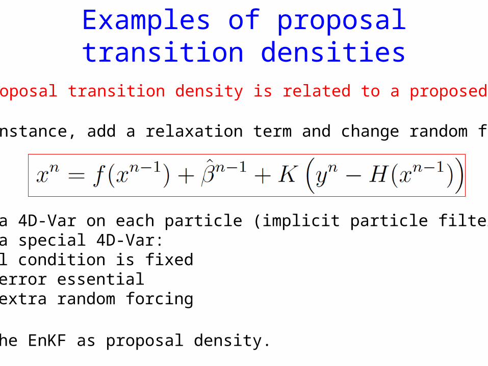
Examples of proposal transition densities
The proposal transition density is related to a proposed model.
For instance, add a relaxation term and change random forcing:
Or, run a 4D-Var on each particle (implicit particle filter). This is a special 4D-Var:- initial condition is fixed- model error essential- needs extra random forcing
Or use the EnKF as proposal density.
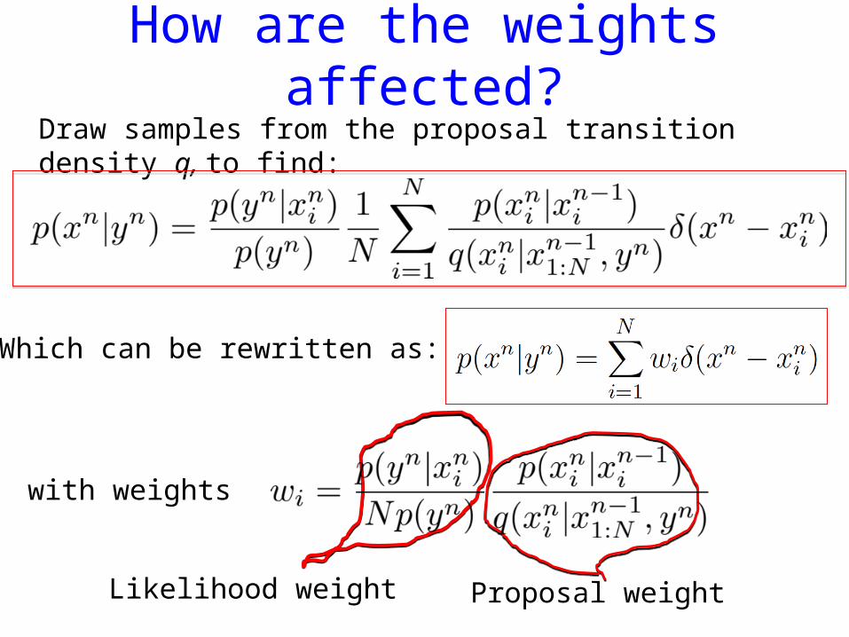
How are the weights affected?
Which can be rewritten as:
with weights
Likelihood weight Proposal weight
Draw samples from the proposal transition density q, to find:
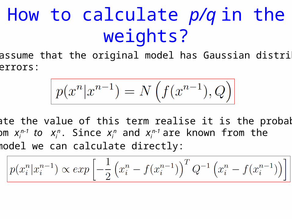
How to calculate p/q in the weights?
Let’s assume that the original model has Gaussian distributedmodel errors:
To calculate the value of this term realise it is the probability ofmoving from xi
n-1 to xin. Since xi
n and xin-1 are known from the
proposed model we can calculate directly:
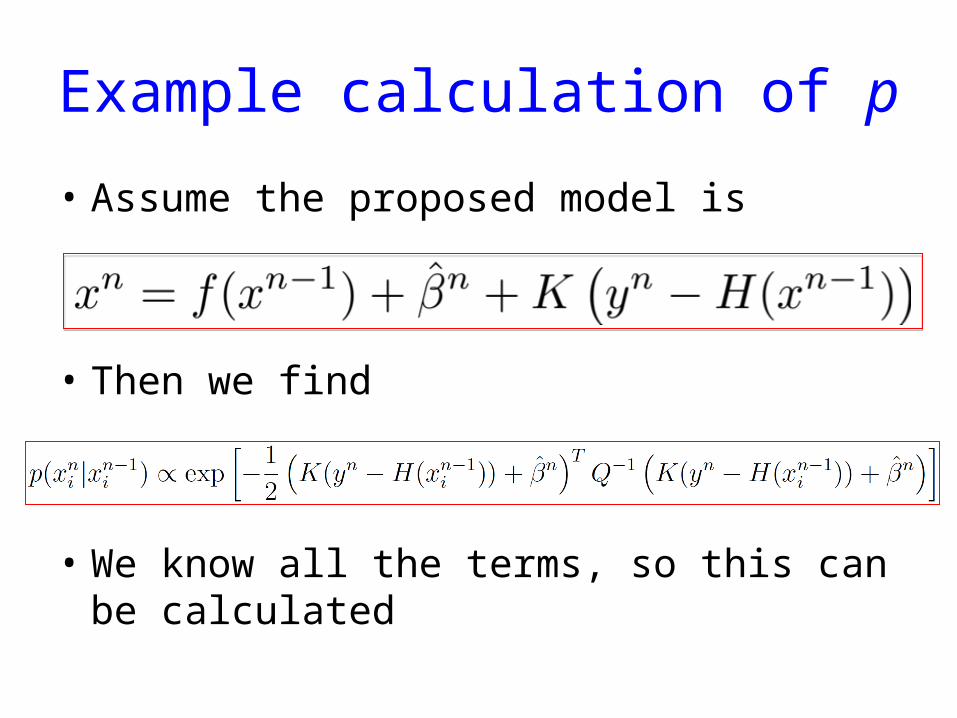
Example calculation of p
• Assume the proposed model is
• Then we find
• We know all the terms, so this can be calculated
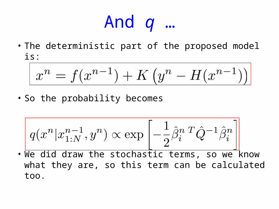
And q …• The deterministic part of the proposed model is:
• So the probability becomes
• We did draw the stochastic terms, so we know what they are, so this term can be calculated too.
• The deterministic part of the proposed model is:
• So the probability becomes
• We did draw the stochastic terms, so we know what they are, so this term can be calculated too.
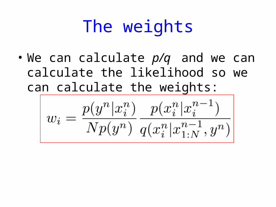
The weights
• We can calculate p/q and we can calculate the likelihood so we can calculate the weights:
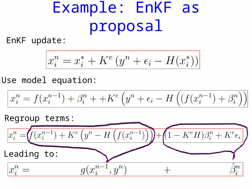
Example: EnKF as proposalEnKF update:
Use model equation:
Regroup terms:
Leading to:
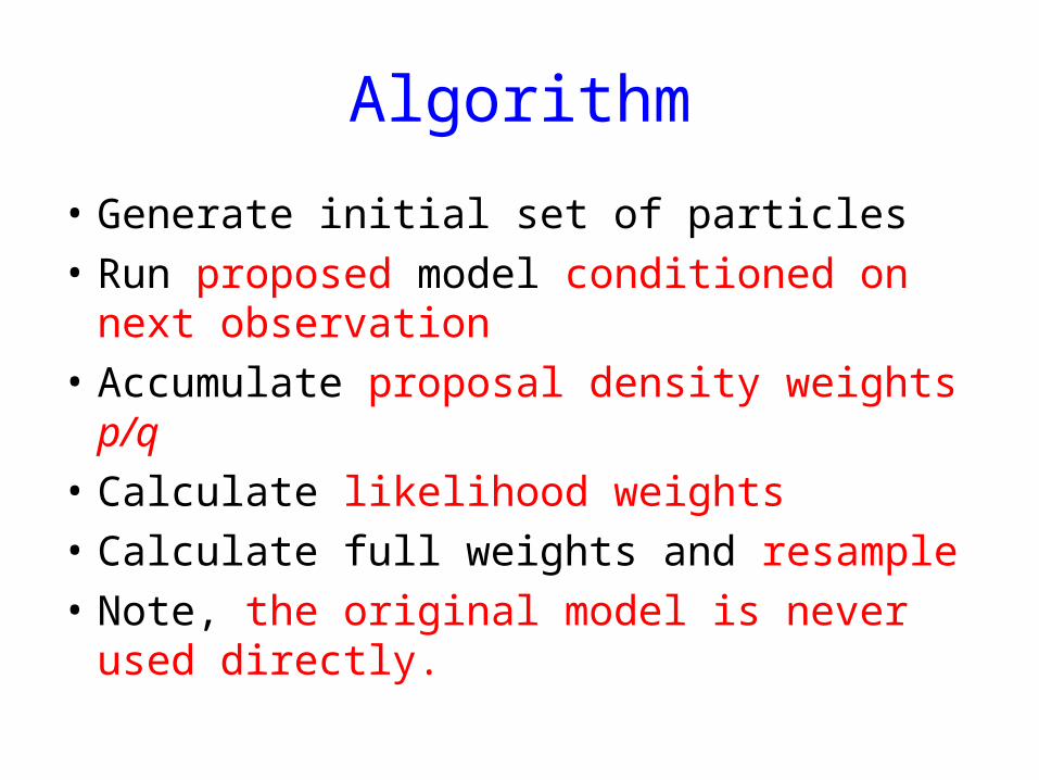
Algorithm
• Generate initial set of particles• Run proposed model conditioned on next
observation• Accumulate proposal density weights p/q• Calculate likelihood weights• Calculate full weights and resample• Note, the original model is never used directly.
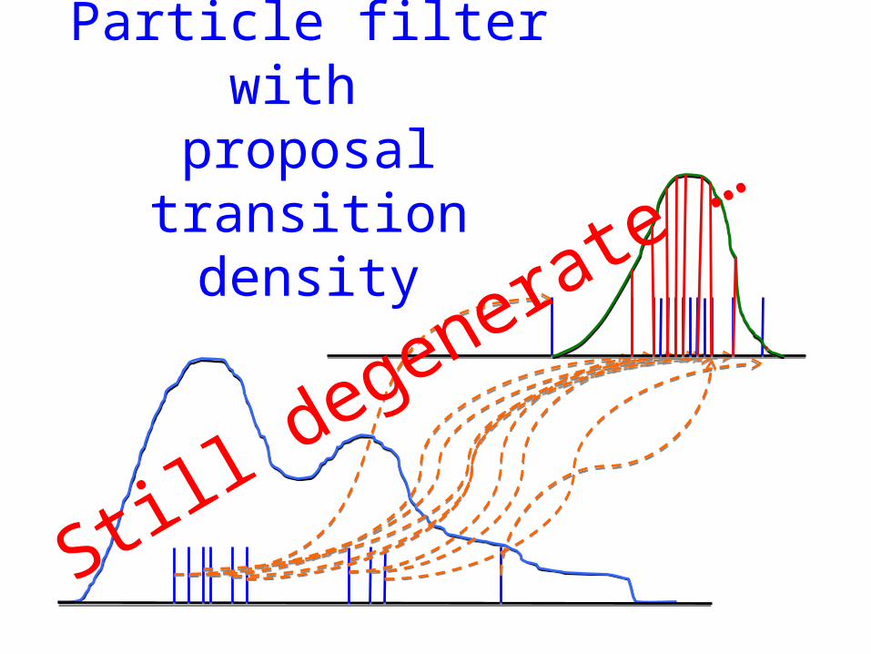
Particle filter with proposal transition
density
Still degenerate …
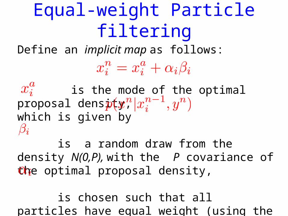
Equal-weight Particle filtering
Define an implicit map as follows:
is the mode of the optimal proposal density,which is given by is a random draw from the density N(0,P), with the P covariance of the optimal proposal density,
is chosen such that all particles have equal weight (using the expression for the weights)

How to find
Remember the new particle is given by:
in which and are known. Use this expressionIn the weights and set all weights equal to a target weight:
and solve for . Now all weights are equal by construction!
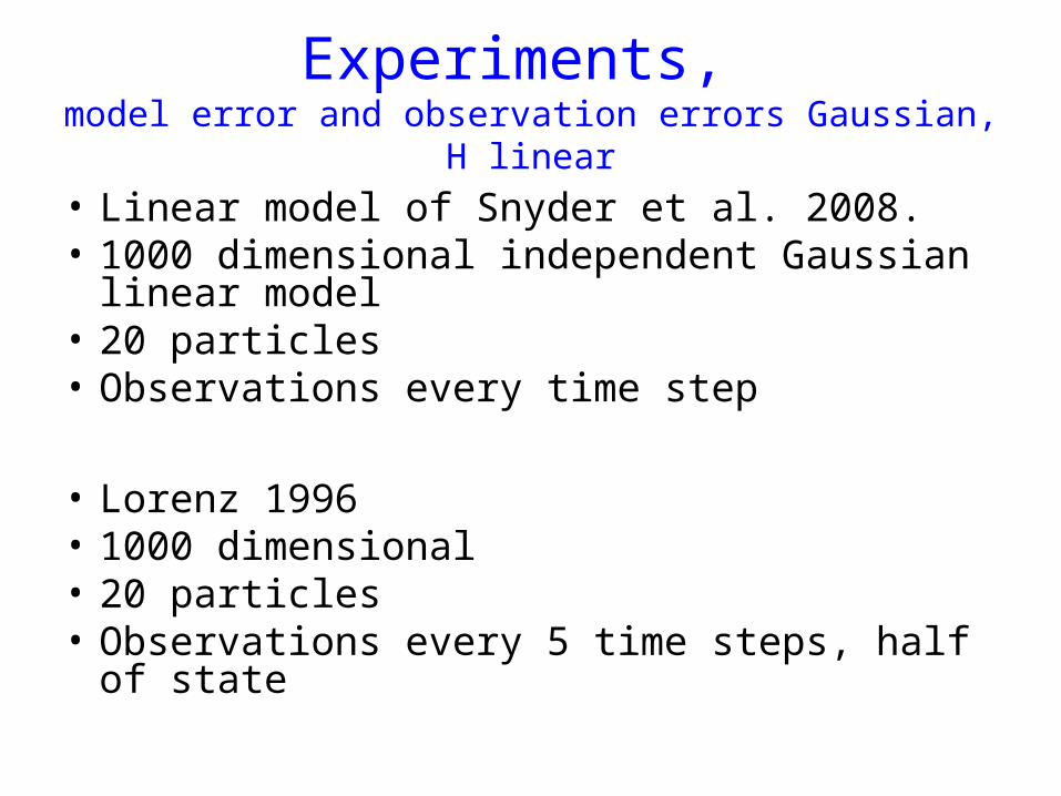
Experiments, model error and observation errors Gaussian, H linear
• Linear model of Snyder et al. 2008.• 1000 dimensional independent Gaussian linear
model• 20 particles• Observations every time step
• Lorenz 1996• 1000 dimensional• 20 particles• Observations every 5 time steps, half of state
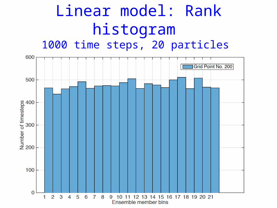
Linear model: Rank histogram 1000 time steps, 20 particles
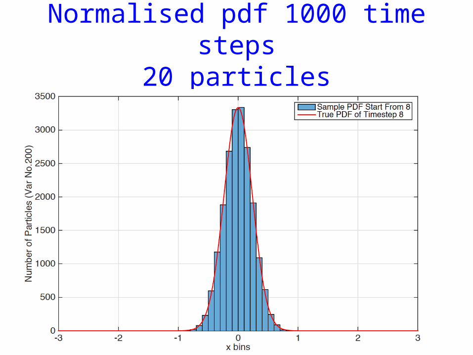
Normalised pdf 1000 time steps20 particles
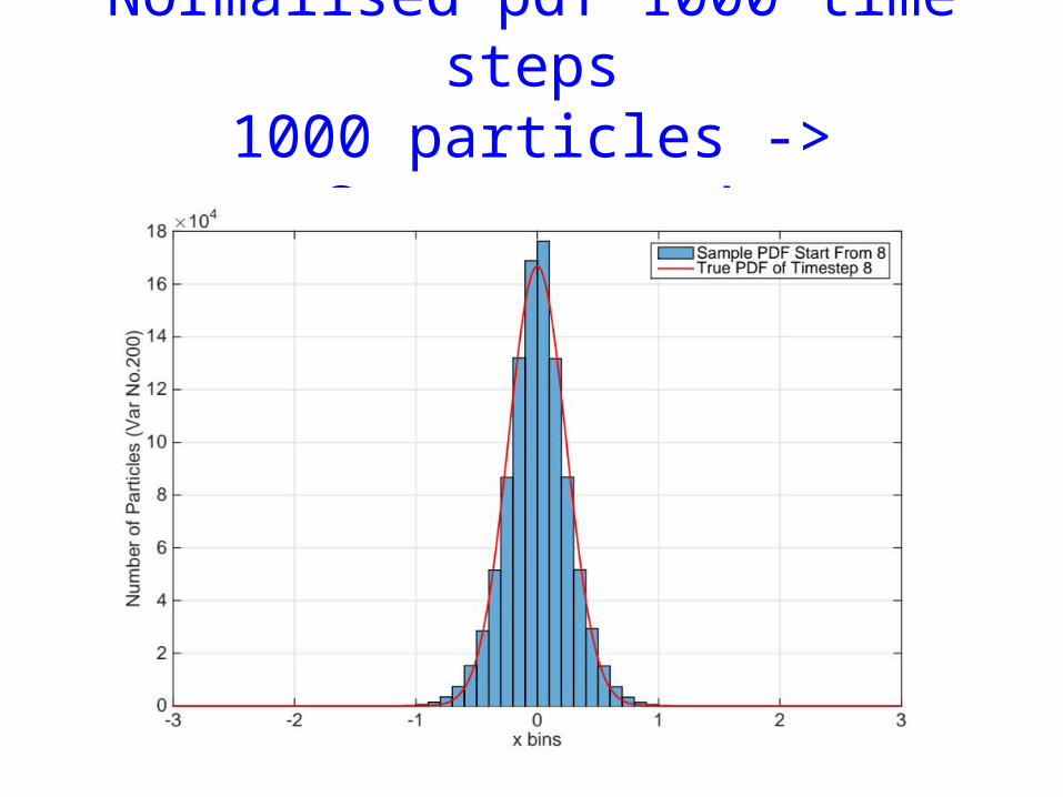
Normalised pdf 1000 time steps1000 particles -> Convergence!
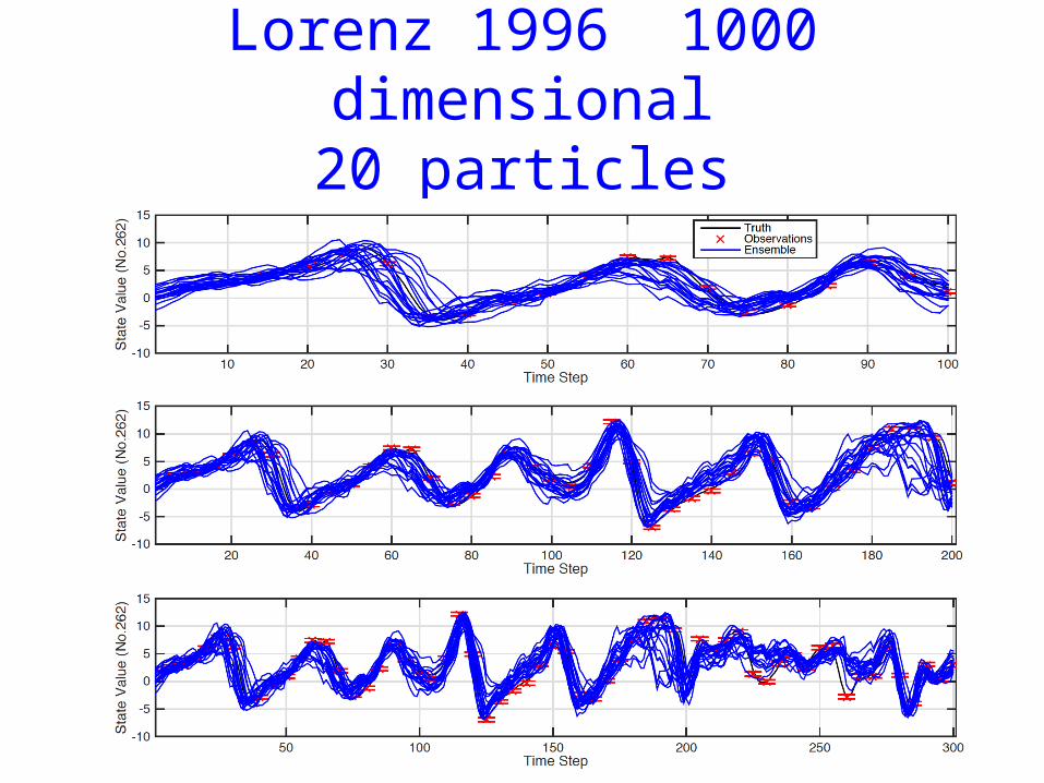
Lorenz 1996 1000 dimensional20 particles
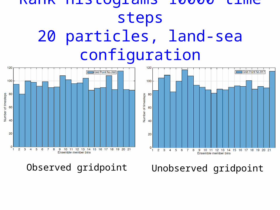
Rank histograms 10000 time steps20 particles, land-sea configuration
Observed gridpoint Unobserved gridpoint
Conclusions• Large number of ‘nonlinear’ filters and smoothers
available• Best method will be system dependent• Fully nonlinear equal-weight particle filters for systems with arbitrary dimensions that converge to the truth posterior pdf do exist.• Proposal-density freedom needs further exploration• Example shown for 1000 dimensional systems, but methods have been applied to 2.3 million dimensional systems too.


