Page 1
Nonlinear Dynamic Modeling and Simulation of a Passively Cooled Small Modular
Reactor
by
Samet Egemen Arda
A Dissertation Presented in Partial Fulfillment
of the Requirements for the Degree
Doctor of Philosophy
Approved November 2016 by the
Graduate Supervisory Committee:
Keith E. Holbert, Chair
John Undrill
Daniel Tylavsky
George Karady
ARIZONA STATE UNIVERSITY
December 2016
Page 2
i
ABSTRACT
A nonlinear dynamic model for a passively cooled small modular reactor (SMR)
is developed. The nuclear steam supply system (NSSS) model includes representations
for reactor core, steam generator, pressurizer, hot leg riser and downcomer. The reactor
core is modeled with the combination of: (1) neutronics, using point kinetics equations
for reactor power and a single combined neutron group, and (2) thermal-hydraulics,
describing the heat transfer from fuel to coolant by an overall heat transfer resistance and
single-phase natural circulation. For the helical-coil once-through steam generator, a
single tube depiction with time-varying boundaries and three regions, i.e., subcooled,
boiling, and superheated, is adopted. The pressurizer model is developed based upon the
conservation of fluid mass, volume, and energy. Hot leg riser and downcomer are treated
as first-order lags. The NSSS model is incorporated with a turbine model which permits
observing the power with given steam flow, pressure, and enthalpy as input. The overall
nonlinear system is implemented in the Simulink dynamic environment. Simulations for
typical perturbations, e.g., control rod withdrawal and increase in steam demand, are run.
A detailed analysis of the results show that the steady-state values for full power are in
good agreement with design data and the model is capable of predicting the dynamics of
the SMR. Finally, steady-state control programs for reactor power and pressurizer
pressure are also implemented and their effect on the important system variables are
discussed.
Page 3
ii
Dedication
To
my beloved Sister
Page 4
iii
ACKNOWLEDGMENTS
First and foremost, I should express my sincere gratitude to Dr. Keith E. Holbert
for accepting me as one of his student and giving me the once-in-a-lifetime opportunity
of studying on this PhD degree level project. As a mentor, his expertise and insight
contributed to my graduate experience considerably. I felt his support, guidance, and
encouragement during every stage of this study, from the start to the end.
I also give special thanks to Dr. John Undrill for his interest and excitement over
the project. He not only helped me about programming but also taught me the importance
of relating the theoretical discussions to real physical systems which expanded my
understanding of what the engineering really means.
I am very grateful to the member of my supervisory committee, Dr. Daniel
Tylavsky and Dr. George Karady, for the consideration to be members of the committee
and allocating their precious time to do that.
Finally, I would like to take this opportunity to express my heartfelt gratitude
towards my sister and her husband in Turkey as well as my relatives for showing their
love, support, and encouragement whenever I needed which contributed significantly to
the fulfillment of a long-held dream.
Page 5
iv
TABLE OF CONTENTS
Page
LIST OF TABLES ................................................................................................................ viii
LIST OF FIGURES ................................................................................................................. ix
CHAPTER
1 INTRODUCTION ............................................................................................... 1
1.1 Motivation .................................................................................................. 1
1.2 Different SMR Designs ............................................................................. 6
1.2.1 NuScale SMR Overview .............................................................. 8
1.3 Research Objectives and Thesis Organization ...................................... 14
2 LITERATURE REVIEW .................................................................................. 15
2.1 Introduction .............................................................................................. 15
2.2 Previous Studies on Dynamic Modeling................................................ 15
3 DEVELOPMENT OF MATHEMATICAL MODELS ................................... 20
3.1 Reactor Core Model ................................................................................. 20
3.1.1 Reactor Neutronics ..................................................................... 20
3.1.2 Reactor Thermal-hydraulics ....................................................... 21
3.2 Hot Leg Riser and Downcomer Region .................................................. 29
Page 6
v
CHAPTER Page
3.3 Steam Generator Model ........................................................................... 30
3.3.1 Governing Equations and Assumptions ...................................... 31
3.3.2 Secondary Side Equations .......................................................... 34
3.3.3 Tube Metal Equations ................................................................. 36
3.3.4 Primary Side Equations .............................................................. 37
3.3.5 Heat Transfer Coefficients and Mean Void Fraction ............... 38
3.3.6 Steam Valve Equation ................................................................ 39
3.3.7 Steam Generator State-space Model .......................................... 39
3.4 Pressurizer Model .................................................................................... 42
3.5 Single SMR Unit Model .......................................................................... 46
3.6 Control Systems ....................................................................................... 48
3.6.1 Reactor Control ........................................................................... 48
3.6.2 Primary Coolant System Pressure Control ................................. 52
4 TESTING THE DYNAMIC MODELS IN MATLAB/SIMULINK .............. 53
4.1 Isolated Reactor Core Model ................................................................... 53
4.1.1 Response to a Step Change in External Reactivity ................... 57
4.1.2 Response to a Step Change in Primary Coolant Inlet
Temperature .......................................................................................... 58
Page 7
vi
CHAPTER Page
4.2 Isolated Steam Generator Model ............................................................. 59
4.2.1 Response to a Step Change in Primary Coolant Inlet
Temperature .......................................................................................... 62
4.2.2 Response to a Step Change in Primary Coolant Flow Rate ..... 63
4.2.3 Response to a Step Change in Feedwater Inlet Temperature ... 64
4.2.4 Response to a Step Change in Steam Valve Opening .............. 65
4.2.5 Comparison of Results ................................................................ 66
4.3 Isolated Pressurizer Model ...................................................................... 67
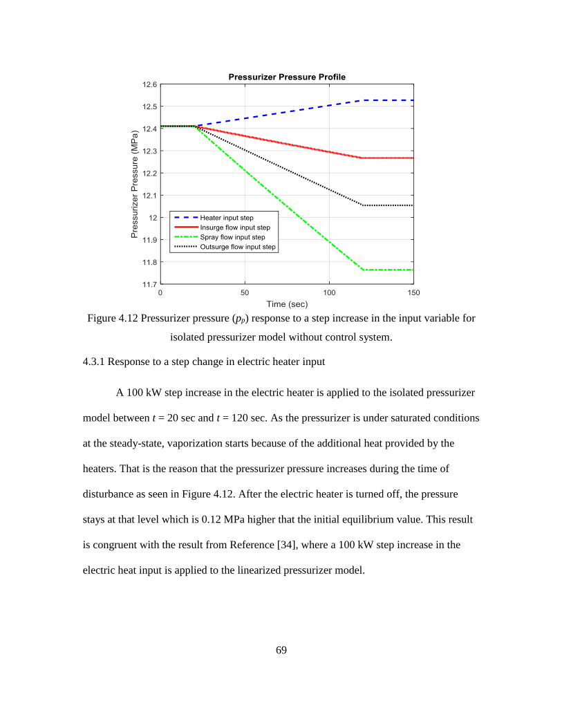
4.3.1 Response to a Step Change in Electric Heater Input ................ 68
4.3.2 Response to a Step Change in Insurge Flow Rate .................... 69
4.3.3 Response to a Step Change in Outsurge Flow Rate.................. 69
4.3.4 Response to a Step Change in Spray Flow Rate ....................... 69
4.3.5 Comparison of Results ................................................................ 70
4.4 Single SMR Unit Model .......................................................................... 71
4.4.1 Steady-state Performance of the Model .................................... 71
4.4.2 Dynamic Performance of the Model .......................................... 73
4.5 Single SMR Unit Model with Control Systems ...................................... 85
4.5.1 Increase in Steam Valve Opening .............................................. 86
Page 8
vii
CHAPTER Page
4.5.2 Increase in Reactor Thermal Power ........................................... 91
5 CONCLUSIONS AND FUTURE WORK ....................................................... 99
5.1 Reseacrh Summary .................................................................................. 99
5.2 Main Results of the Study ..................................................................... 100
5.3 Future Work ........................................................................................... 101
REFERENCES ................................................................................................................... 102
APPENDIX
A REACTOR CORE PARAMETERS AND CALCULATIONS ................. 108
B STEAM GENERATOR PARAMETERS AND CALCULATIONS ......... 114
C HOT LEG RISER, DOWNCOMER, PRESSURIZER AND STEAM ....... 128
D LINEARIZATION ........................................................................................ 134
Page 9
viii
LIST OF TABLES
Table Page
1.1 Design Features of NuScale SMR ................................................................... 11
3.1 Parameters Used to Calculate Fuel-to-coolant Thermal Resistance ............. 24
3.2 Elements of Matrix D(x,u) .............................................................................. 41
4.1 Comparison of Results for Isolated Steam Generator Model without Control
Systems ............................................................................................................. 67
4.2 Comparison of Results for Isolated Pressurizer Model without Control
Systems ........................................................................................................71
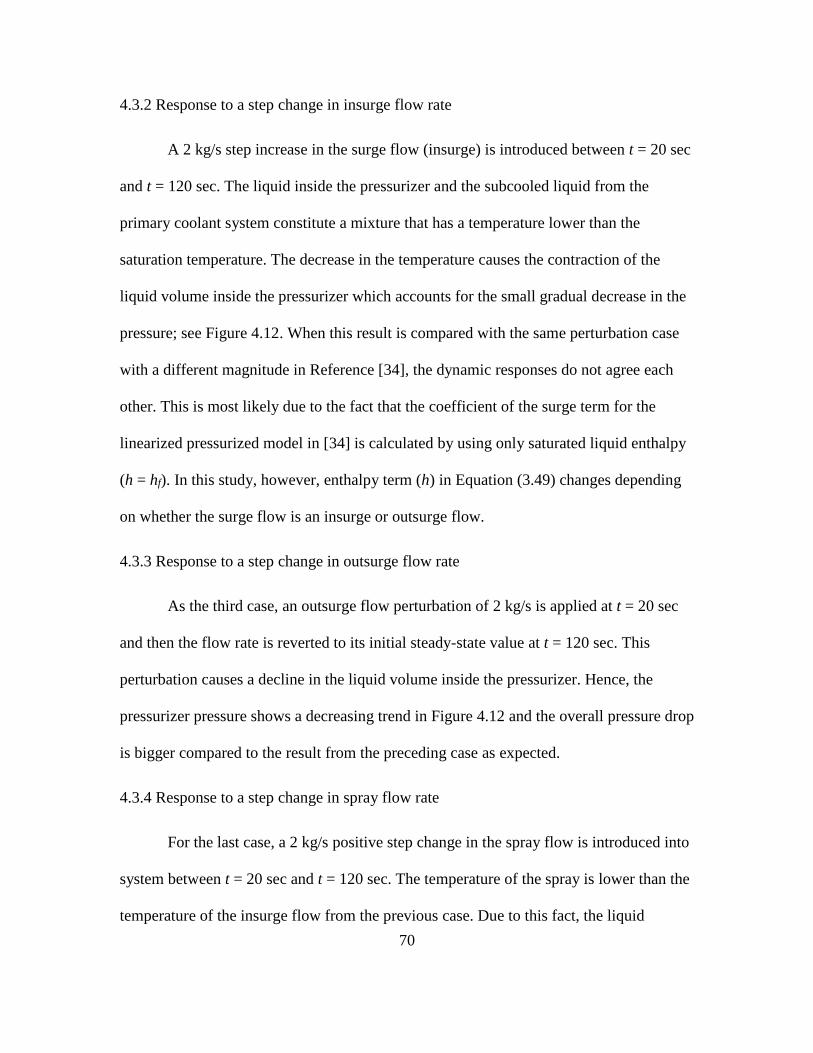
4.3 Steady-state Values of Important Parameters ................................................ 73
A.1 Reactor Core Parameters .............................................................................. 110
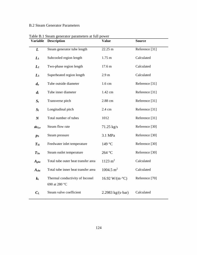
B.1 Steam Generator Parameters at Full Power ................................................. 124
C.1 Hot Leg Riser, Downcomer, Pressurizer, and Steam Turbine
Parameters ..................................................................................................... .130
D.1 Elements of Matrix Fx ................................................................................139
D.2 Elements of Matrix Fu ...............................................................................141
Page 10
ix
LIST OF FIGURES
Figure Page
1.1 Electrical Output of U.S. Commercial Nuclear Power Plants [6] .................. 2
1.2 Schematic Diagram of a Single NuScale SMR Unit ..................................... 10
1.3 Cross-sectional View of NuScale Reactor Core ............................................ 12
1.4 Photo of NuScale Full-length Helical Coil Steam Generator [32] ............... 13
3.1 Schematic Diagram of Heat Transfer Model in Reactor Core ...................... 22
3.2 Schematic Diagram of NuScale SMR ............................................................ 27
3.3 Schematic Diagram of Helical-coil Steam Generator Model ....................... 32
3.4 Schematic Diagram of Pressurizer Model ...................................................... 43
3.5 Simulink Representation of Overall Reactor Model ..................................... 47
3.6 Characteristics of Constant-average-temperature Control Model ...............49
3.7 Characteristics of a Constant-steam-pressure Control Mode ......................50
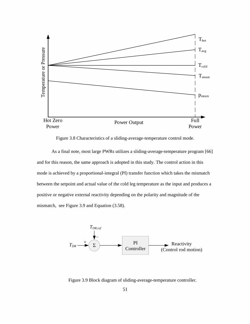
3.8 Characteristics of a Sliding-average-temperature Control Mode ................51
3.9 Block Diagram of Sliding-average-temperature Controller ........................51
3.10 Block Diagram of Pressurizer Pressure Controller ......................................52
4.1 Reactor Power (P) Response to a Step Increase in the Input Variable for
Isolated Reactor Core Model .......................................................................... 55
4.2 Fuel Temperature (TF) Response to a Step Increase in the Input Variable for
Isolated Reactor Core Model .......................................................................... 55
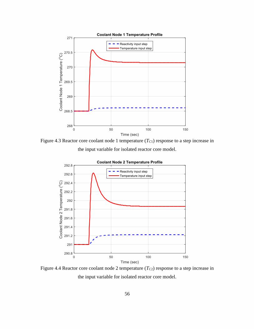
4.3 Reactor Core Coolant Node 1 Temperature (TC1) Response to a Step
Increase in the Input Variable for Isolated Reactor Core Model.................. 56
Page 11
x
Figure Page
4.4 Reactor Core Coolant Node 2 Temperature (TC2) Response to a Step
Increase in the Input Variable for Isolated Reactor Core Model.................. 56
4.5 Primary Coolant Mass Flow Rate (ṁC) Response to a Step Increase in the
Input Variable for Isolated Reactor Core Model ........................................... 57
4.6 System Reactivity (ρ) Response to a Step Increase in the Input Variable for
Isolated Reactor Core Model .......................................................................... 57
4.7 Subcooled Region Length (L1) Response to a Step Increase in the Input
Variable for Isolated Steam Generator Model ............................................... 60
4.8 Two-phase Region Length (L2) Response to a Step Increase in the Input
Variable for Isolated Steam Generator Model ............................................... 61
4.9 Superheated Region Length (L3) Response to a Step Increase in the Input
Variable for Isolated Steam Generator Model ............................................... 61
4.10 Steam Pressure (pS) Response to a Step Increase in the Input Variable for
Isolated Steam Generator Model .................................................................... 62
4.11 Primary Coolant Outlet Temperature (TP1) Response to a Step Increase in
the Input Variable for Isolated Steam Generator Model ..............................62
4.12 Pressurizer Pressure (pp) Response to a Step Increase in the Input Variable
for Isolated Pressurizer Model without Control System ..............................69
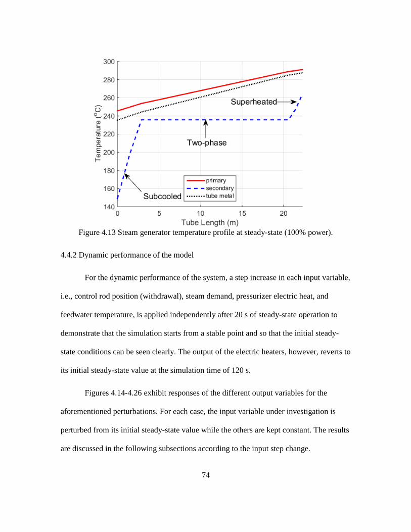
4.13 Steam Generator Temperature Profile at Steady-state (100% power) .........74
4.14 Reactor Power (P) Response to a Step Increase in the Input Variable for
Single SMR Unit ..........................................................................................75
Page 12
xi
Figure Page
4.15 Fuel Temperature (TF) Response to a Step Increase in the Input Variable for
Single SMR Unit ..........................................................................................75
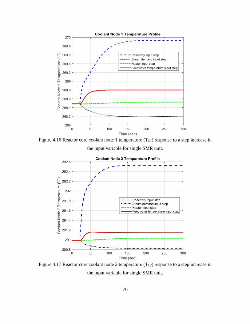
4.16 Reactor Core Coolant Node 1 Temperature (TC1) Response to a Step
Increase in the Input Variable for Single SMR Unit ...................................76
4.17 Reactor Core Coolant Node 2 Temperature (TC2) Response to a Step
Increase in the Input Variable for Single SMR Unit ..................................... 76
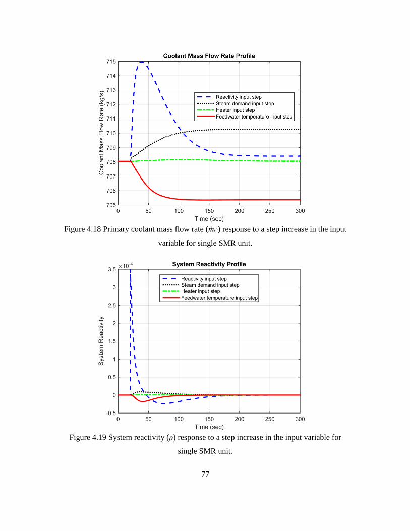
4.18 Primary Coolant Mass Flow Rate (ṁC) Response to a Step Increase in the
Input Variable for Single SMR Unit .............................................................. 77
4.19 System Reactivity (ρ) Response to a Step Increase in the Input Variable for
Single SMR Unit ............................................................................................. 77
4.20 Subcooled Region length (L1) Response to a Step Increase in the Input
Variable for Single SMR Unit ........................................................................ 78
4.21 Two-phase Region Length (L2) Response to a Step Increase in the Input
Variable for Single SMR Unit ........................................................................ 78
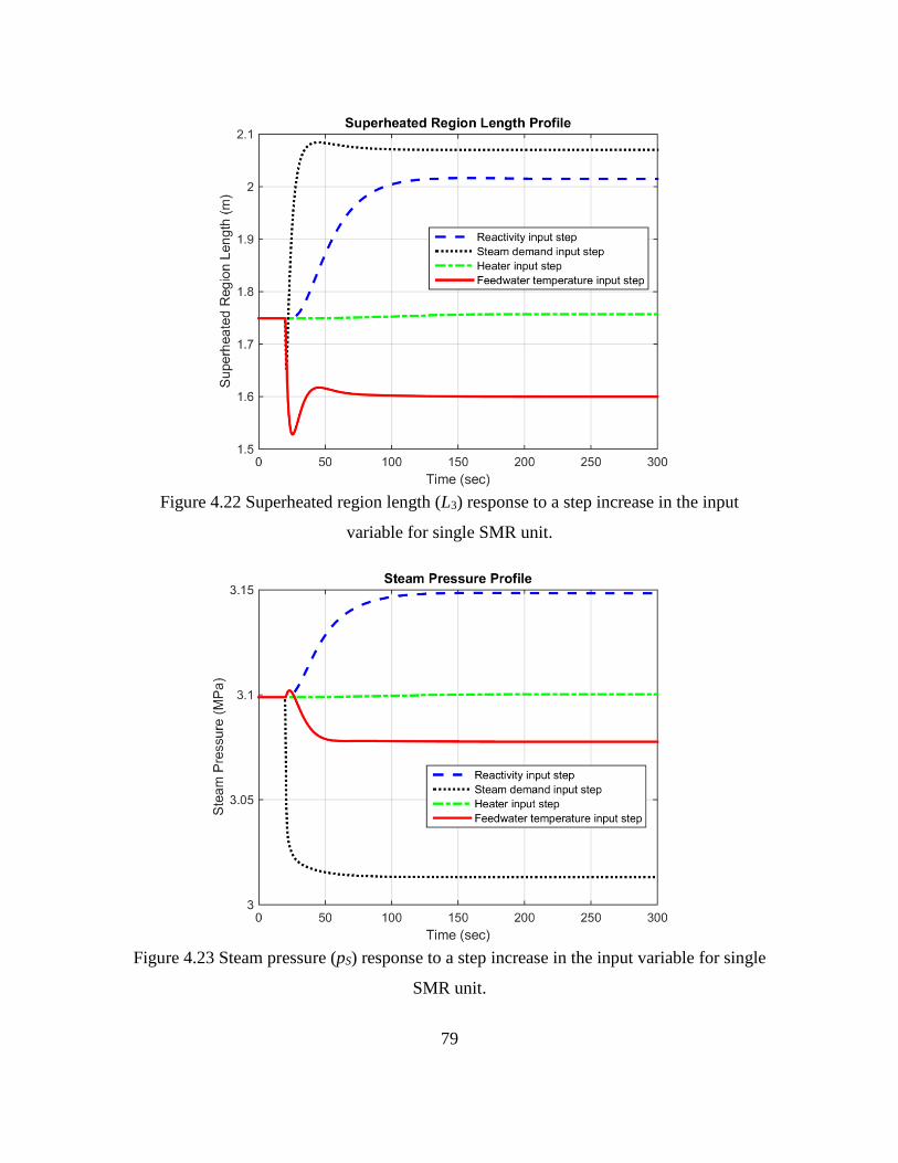
4.22 Superheated Region Length (L3) Response to a Step Increase in the Input
Variable for Single SMR Unit ........................................................................ 79
4.23 Steam Pressure (pS) Response to a Step Increase in the Input Variable for
Single SMR Unit ............................................................................................. 79
4.24 Primary Coolant Temperature (TP1) Response at the Steam Generator Outlet
to a Step Increase in the Input Variable for Single SMR Unit ..................... 80
4.25 Pressurizer Pressure (pp) Response to a Step Increase in the Input Variable
for Single SMR Unit ....................................................................................... 80
Page 13
xii
Figure Page
4.26 Maximum Attainable Power (Pm) Response to a Step Increase in the Input
Variable for Single SMR Unit ........................................................................ 81
4.27 Thermal Power (P) Response for a Step Increase in the Load for Single
SMR Unit with and without Control Systems .............................................87
4.28 Change in Primary Coolant Temperatures for a Step Increase in the Load
for Single SMR Unit without Control Systems ...........................................88
4.29 Change in Primary Coolant Temperatures for a Step Increase on the Load
for Single SMR Unit with Control Systems ................................................88
4.30 Pressurizer Pressure (pP) Response for a Step Increase in the Load for
Single SMR Unit with and without Control Systems ..................................89
4.31 Steam Pressure (pS) Response for a Step Increase in the Load for Single
SMR Unit with and without Control Systems .............................................89
4.32 Maximum Attainable Power (Pm) Response for a Step Increase in the Load
for Single SMR Unit with and without Control Systems ............................90
4.33 Change in Thermal and Maximum Attainable Power for a Step Increase in
the Load for Single SMR Unit with Control Systems .................................90
4.34 Thermal Power (P) Response for a Ramp Increase in Reactor Power
Controller Reference Value for Single SMR Unit .......................................93
4.35 Fuel Temperature (TF) Response for a Ramp Increase in Reactor Power
Controller Reference Value for Single SMR Unit .......................................94
Page 14
xiii
Figure Page
4.36 Reactor Core Coolant Node 2 Temperature (TC2) Response for a Ramp
Increase in Reactor Power Controller Reference Value for Single SMR
Unit ..............................................................................................................94
4.37 Primary Coolant Mass Flow Rate (ṁC) Response for a Ramp Increase in
Reactor Power Controller Reference Value for Single SMR Unit ..............95
4.38 Normalized Temperature Difference (TC2/TC2,0 – TCi/TCi,0) for a Ramp
Increase in Reactor Power Controller Reference Value for Single SMR
Unit ..............................................................................................................95
4.39 System Reactivity (ρ) Response for a Ramp Increase in Reactor Power
Controller Reference Value for Single SMR Unit .......................................96
4.40 Steam Pressure (pS) Response for a Ramp Increase in Reactor Power
Controller Reference Value for Single SMR Unit .......................................96
4.41 Pressurizer Pressure (pp) Response for a Ramp Increase in Reactor Power
Controller Reference Value for Single SMR Unit .......................................97
4.42 Maximum Attainable Power (Pm) Response for a Ramp Increase in Reactor
Power Controller Reference Value for Single SMR Unit ............................97
A.1 Equivalent Coolant Channels in a Square Fuel Lattice ............................... 112
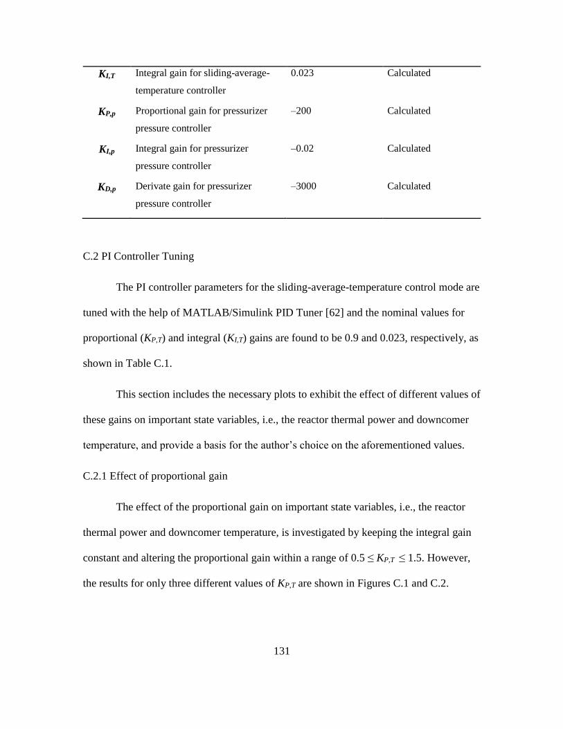
C.1 Effect of Proportional Gain (KP,T) on Reactor Thermal Power..................132
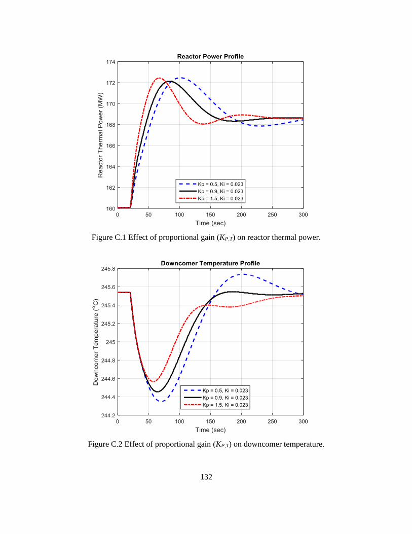
C.2 Effect of Proportional Gain (KP,T) on Downcomer Temperature .............132
C.3 Effect of Integral Gain (KI,T) on Reactor Thermal Power..........................133
C.4 Effect of Integral Gain (KI,T) on Downcomer Temperature .......................134
Page 15
1
CHAPTER 1 INTRODUCTION
1.1 Motivation
A small reactor, defined by the International Atomic Energy Agency (IAEA), is a
nuclear reactor with an output of less than 300 MWe [1]. The term “modular” is derived
from the fact that small reactors can be manufactured in a factory completely and
delivered to the site for installation.
The first commercial nuclear power plant in the U.S. was the Shippingport
Atomic Power Station with a total capacity of 60 MWe [2]. The plant, which was located
40 km away from Pittsburg, reached critically on December 2, 1957 and was able to
produce electricity on December 18, 1957. Since then, the capacity of a single reactor has
been increased up to around 1600 MWe considering economy of scale (see Figure 1.1).
However, even in the 1960s when the trend was toward larger plant sizes, the potential of
SMRs was being considered [3]. Starting with the late 1970s in the U.S., new projects for
construction of nuclear power plants mostly have been postponed or canceled due to high
initial investments, construction period exceeding 10 years, and cumbersome licensing
process [4]. In fact, for the first time after almost 35 years, the Nuclear Regulatory
Commission (NRC) approved construction and operation licenses for units 3 and 4 of the
Alvin W. Vogtle Electric Generating Plant on February 10, 2012. Prior to that, the last
construction permit for a nuclear power plant was issued in 1978 for the Shearon Harris
Nuclear Power Plant located in New Hill, North Carolina [5].
Page 16
2
Figure 1.1 Electrical output of U.S. commercial nuclear power plants [6].
Starting in the last decade, there has been a growing trend in the development and
commercialization of small modular reactors (SMRs) not only in the U.S. but also in
other countries including Russia, Japan, France, India, Argentina, South Korea, and
China. However, these SMRs are not intended to be scaled-down version of today’s large
nuclear reactors. The key in this scramble is to create a unique design, primarily, with the
idea of combining steam generators and pressurizer with the reactor core in the reactor
pressure vessel which is described with the term ‘integral’. Furthermore, lessons learned
from 60 years of nuclear engineering and tragic accidents such as Three Mile Island,
Chernobyl, and Fukushima compel the industry to develop intrinsically safer and more
secure reactors.
To support U.S.-based SMR projects, the Department of Energy (DOE) launched
a program called SMR Licensing Technical Support Program in March 2012 [7].
According to this 6-year 452 million dollars cost-share public-private partnership, two
Page 17
3
industry members were each awarded with half of the total funding. The first half of the
funding was provided to a consortium led by Babcock & Wilcox (B&W) and including
the Tennessee Valley Authority and Bechtel on November 20, 2012 [8]. Approximately
one year later, DOE announced on December 12, 2013 that NuScale Power LLC would
be the company receiving the second half of the funding [9]. Different design features of
these two companies’ SMRs will be discussed later.
SMRs can be utilized to supply the electricity needs of remote areas suffering
from the lack of transmission and distribution infrastructure and also generate local
power for particular regions within large population centers. In addition, SMR
technology presents an ideal opportunity for small countries where the power demand
does not change significantly and countries facing problems with high initial investments
associated with large nuclear power plants [10]. However producing electricity is not the
only area where SMRs are applicable. Other applications including: water desalination,
general process heat for chemical or manufacturing processes, and district heating are
also possible with appropriate design.
Advantages of SMRs can be categorized into four groups [11]:
1. Fabrication and construction,
2. Plant safety,
3. Operational flexibility, and
4. Economics.
Fabrication and construction: Parallel with power outputs of SMRs, the physical
size of major components in a reactor shrinks which provides simplicity in manufacturing
Page 18
4
by reducing or eliminating the need for forging and requires less advanced technology.
Utilizing conventional fabrication methods is very important since the technology is a
limiting factor causing large nuclear reactors to be manufactured by a few vendors
throughout the world. Another problem related to employing large reactor vessel is
transportation. Often, reactor vessel size imposes restrictions on possible options for plant
location and forces it to be located near the shore of a sea or a large river. On the
contrary, SMRs can be transported by a ship, ferry, rail, or even truck and sat onto inland
areas or remote locations. Lastly, large nuclear power plants require great amount of on-
site work that both increases cost and can cause delays in scheduled construction plan.
With SMRs, a higher percentage of a plant can be built in a factory and delivered to the
plant site for installation. This also can improve the quality of various components as a
result of quality control means of a factory environment.
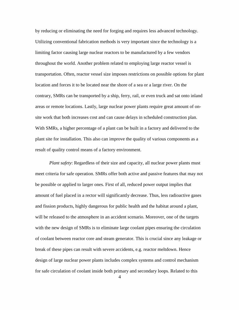
Plant safety: Regardless of their size and capacity, all nuclear power plants must
meet criteria for safe operation. SMRs offer both active and passive features that may not
be possible or applied to larger ones. First of all, reduced power output implies that
amount of fuel placed in a rector will significantly decrease. Thus, less radioactive gases
and fission products, highly dangerous for public health and the habitat around a plant,
will be released to the atmosphere in an accident scenario. Moreover, one of the targets
with the new design of SMRs is to eliminate large coolant pipes ensuring the circulation
of coolant between reactor core and steam generator. This is crucial since any leakage or
break of these pipes can result with severe accidents, e.g. reactor meltdown. Hence
design of large nuclear power plants includes complex systems and control mechanism
for safe circulation of coolant inside both primary and secondary loops. Related to this
Page 19
5
aspect, placing steam generator and pressurizer inside reactor vessel will increase the
height of the overall system facilitating natural circulation of coolant in a reactor. Finally,
due to the size of a SMR, reactors in a plant can be placed into pools under surface level.
That provides additional resistance against terror attacks and pools serve as a heat sink
for removing the decay heat by radionuclides after a reactor shutdown or in an emergency
situation.
Operational flexibility: Nuclear power plants with SMRs compared to ones with
large reactors have a smaller footprint, thus, reducing the size of the emergency planning
zone [11]. This fact improves the flexibility on site selection and allows reactors to be
placed near industrial areas and population centers. A plant site closer to potential
customers is very important if the reactor will be utilized for process heat or district
heating. Another advantage is that it reduces losses owing to long transmission and
distribution lines if the purpose is to produce electricity.
SMRs are also favorable for water usage since less electric output implies less
heat rejection to the environment. Thus water demand decreases and the plant does not
require a sea or a large river. In addition, reduced dependency on a big water supply is
another factor contributing the site selection flexibility.
The other advantage is that smaller capacity and reduced construction time allows
matching growth in power demand closely and increasing the power output of a plant
incrementally which also impacts plant economics as will be discussed below.
Economics: A typical value for the total cost of a large nuclear power plant is
about 10 billion dollars. This is a big capital investment which directly eliminates many
Page 20
6
small countries and private utilities from involvement with nuclear industry. However,
SMRs enable those countries to start their own nuclear program and utilities to own a
nuclear power plant within the local grid they are responsible for.
As mentioned above, the “economy of scale” principle encourages a reactor with
higher electrical output but this fact, nevertheless, does not mean that SMRs are not
economically viable. In fact, results of a study [12] conclude that the economy of scale
law could be overcome by other SMR features such as modularization and lower upfront
cost. These features increase SMR competitiveness over large reactors. For example, in
case of a nuclear power plant comprising four SMRs, the construction plan can be
organized in a way that each reactor is built after the preceding one is complete. In other
words, when the first unit starts generating revenue, the second one comes into
production line. As a result, cash outflow significantly drops reducing the risk related to
high initial investment of large nuclear power plants.
1.2 Different SMR Designs
Different companies from different parts of the world have various unique designs
and configurations for SMRs. A brief summary of some of them is provided below:
CAREM-25 is a prototype reactor and currently being built 110 km northwest of
Buenos Aires by the Argentine National Atomic Energy Commission (CNEA) with the
help of INVAP in Lima [13]. CAREM-25 is a 100 MWt (27 MWe) light-water
pressurized water reactor (PWR) and the design concept was first introduced in 1984
[14]. Natural circulation provides the reactor core cooling and the reactor vessel
encompasses 12 vertical helical-coil steam generators. The most prominent feature of
Page 21
7
CAREM-25 is that the reactor does not have a pressurizer. The balance between the
vaporization in the hot leg and the condensation of vapor due to the colder structures in the
steam dome achieves self-pressurization in the primary system [15].
HTR-10 is a high-temperature gas-cooled research reactor with 10 MWt output
developed at the Institute of Nuclear & New Energy Technology (INET) in China [16]. It
is a modular pebble bed type reactor. The reactor core consists of 2700 spherical fuel
elements of UO2 and each of them has 5 g of heavy metal. In this design, graphite is used
as reflector and helium as coolant. Cooler helium at the inlet with a temperature of
250 °C flows from top to bottom of the pebble bed reactor core and it reaches to up to a
temperature of 700 °C at the outlet. HTR-10 is not an integral type reactor and the steam
generator is connected to the reactor pressure vessel by hot gas duct. The steam generator
is a once-through steam generator comprised of 30 helical-coil tube bundles [17]. HTR-
10 paved the way for a larger version of its design called HTR-PM. The construction of a
power plant comprising two HTR-PMs, each 250 MWt, driving a single 201 MWe steam
turbine began in December 2012 at Rongcheng in Shandong province in China. The plant
is scheduled be online by 2015 [13].
SMART (System-integrated Modular Advanced Reactor) is a 330 MWt integral
reactor developed by Korea Atomic Energy Research Institute (KAERI) [18]. SMART is
designed for electricity generation (110 MWe) as well as seawater desalination. The
reactor core is cooled with the help of four coolant pumps. The design data indicate the
coolant temperature increases by 40 °C while passing through the reactor core
Page 22
8
corresponding to a core outlet temperature of 310 °C. The reactor vessel houses 8 helical-
coil once-through steam generators [19].
The first DOE sponsored design, B&W’s mPower, is developed based upon the
knowledge and experience gained by the B&W maritime reactor program. One of these
earlier designs is used in Otto Hahn, a nuclear powered merchant ship launched in 1964
[20]. mPower is an integral reactor with an output of 530 MWt. Net electricity generation
changes according to type of condenser cooling employed—mPower is expected to
produce 180 MWe when evaporative cooling is utilized whereas deploying an air-cooled
unit reduces the electrical output to 155 MW. The reactor coolant flow rate relies on
forced circulation by eight internal coolant pumps [21], [22].
Other U.S.-based SMRs being developed include the Westinghouse SMR, Holtec
SMR-160, and PRISM (Power Reactor Innovative Small Module) by a consortium of
General Electric and Hitachi [23]-[26]. The Westinghouse SMR and Holtec SMR-160 are
PWRs with electrical outputs of 225 MW and 160 MW, respectively. PRISM, on the
other hand, is a sodium-cooled fast neutron reactor expected to produce 311 MWe.
1.2.1 NuScale SMR overview
A detailed overview of the NuScale SMR is provided in this section since its
design data are used throughout the modeling effort and dynamic analyses of this
dissertation. However, the generic approach adopted in this research can be applied for
passively cooled SMRs.
The NuScale SMR, capable of producing 45 MWe, is based on the Multi-
Application Small Light Water Reactor (MASLWR) concept which was developed by a
Page 23
9
consortium including Idaho National Laboratory and Oregon State University under a
DOE-sponsored project [27].
Each nuclear steam supply system (NSSS), as seen in Figure 1.2, is immersed in a
reactor pool, which has dimensions of 6 m wide by 6 m long and a depth of 23 m. The
reactor pressure vessel is housed in the containment vessel sitting inside the reactor pool.
The integral design allows the NSSS to encompass all major components, which are the
reactor core, two helical-coil once-through steam generators, and pressurizer [28].
Table 1.1 provides a summary of NuScale SMR design features [29].
Page 24
10
Containment
Vessel
Steam
Generator
Reactor Core
Downcomer
Hot Leg
Riser
Pressurizer
Control Rod
Drives
Reactor Pressure
Vessel
Control Rods
Baffle Plate
Figure 1.2 Schematic diagram of a single NuScale SMR unit.
Page 25
11
Table 1.1 Design features of NuScale SMR
Parameters Value
Reactor thermal power 160 MWt
Power plant output, net 45 MWe
Coolant/Moderator Light water
Circulation type Natural circulation
Reactor operating pressure 12.76 MPa
Active core height 2 m
Fuel material UO2 ceramic pellets
Fuel element type 17×17, square array
Cladding material Zircaloy-4
U-235 enrichment < 4.95%
Fuel cycle length 24 months
Steam generator type Vertical, helical-coil
Number of steam generators 2
Pressurizer type Integral
The NuScale SMR design employs natural circulation for the primary coolant
system and therefore eliminates reactor coolant pumps. The primary coolant is heated as
it passes over the fuel rods and enters the hot leg riser where convection and natural
buoyancy provide enough force to drive the fluid upward. After leaving the riser, the
primary coolant follows a downward path over the steam generator tubes and the heat is
transferred to the feedwater. The denser primary coolant reaches the bottom of the core
via the downcomer.
Page 26
12
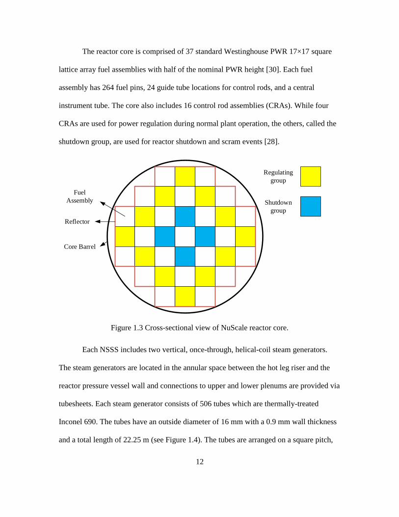
The reactor core is comprised of 37 standard Westinghouse PWR 17×17 square
lattice array fuel assemblies with half of the nominal PWR height [30]. Each fuel
assembly has 264 fuel pins, 24 guide tube locations for control rods, and a central
instrument tube. The core also includes 16 control rod assemblies (CRAs). While four
CRAs are used for power regulation during normal plant operation, the others, called the
shutdown group, are used for reactor shutdown and scram events [28].
Regulating
group
Shutdown
group
Core Barrel
Reflector
Fuel
Assembly
Figure 1.3 Cross-sectional view of NuScale reactor core.
Each NSSS includes two vertical, once-through, helical-coil steam generators.
The steam generators are located in the annular space between the hot leg riser and the
reactor pressure vessel wall and connections to upper and lower plenums are provided via
tubesheets. Each steam generator consists of 506 tubes which are thermally-treated
Inconel 690. The tubes have an outside diameter of 16 mm with a 0.9 mm wall thickness
and a total length of 22.25 m (see Figure 1.4). The tubes are arranged on a square pitch,
Page 27
13
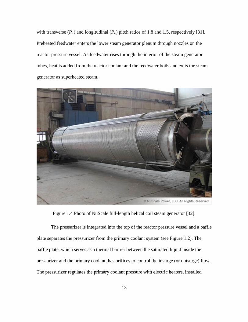
with transverse (PT) and longitudinal (PL) pitch ratios of 1.8 and 1.5, respectively [31].
Preheated feedwater enters the lower steam generator plenum through nozzles on the
reactor pressure vessel. As feedwater rises through the interior of the steam generator
tubes, heat is added from the reactor coolant and the feedwater boils and exits the steam
generator as superheated steam.
Figure 1.4 Photo of NuScale full-length helical coil steam generator [32].
The pressurizer is integrated into the top of the reactor pressure vessel and a baffle
plate separates the pressurizer from the primary coolant system (see Figure 1.2). The
baffle plate, which serves as a thermal barrier between the saturated liquid inside the
pressurizer and the primary coolant, has orifices to control the insurge (or outsurge) flow.
The pressurizer regulates the primary coolant pressure with electric heaters, installed
Page 28
14
above the baffle plate, and spray through nozzles at the top of the reactor pressure vessel.
An increase in the coolant pressure is accomplished by actuating electric heaters while
the coolant pressure is reduced by spraying cold water from the chemical and volume
control system. Unlike traditional PWR pressurizers, a continuous spray flow is not
anticipated.
1.3 Research Objectives and Thesis Organization
The main objectives of this study are based upon the following:
To develop a dynamic model in MATLAB/Simulink for the a passively cooled
SMR (such as the NuScale SMR) which is capable of predicting the response of
the SMR for typical perturbations; and
To verify whether the model is realistic or not by comparing the results gathered
from other studies.
To introduce and apply steady-state control algorithms for reactor power and
pressurizer pressure.
After this introduction, a review of relevant literature is presented in Chapter 2.
While Chapter 3 describes the mathematical models of real physical systems in single
SMR unit, Chapter 4 is composed of testing the model in the dynamic environment of
Matlab/Simulink. Lastly, Chapter 5 is dedicated to concluding remarks and future work.
Page 29
15
CHAPTER 2 LITERATURE REVIEW
2.1 Introduction
Understanding reactor dynamics is crucial to the overall performance of a reactor
and the design of suitable control algorithms. That is the reason dynamic modeling
attracts a great interest in the nuclear industry.
With the increasing effort into development and commercialization of SMRs, the
need for appropriate dynamic models emerges. Although studies regarding individual
components of an SMR, i.e., reactor core, steam generator, and pressurizer, are available,
there is a lack of complete models for single SMR units in the literature. In addition,
different SMR designs require different considerations. In other words, the modeling
endeavor is subject to change based on reactor configuration and operation. Considering
the problems stated above, a representation for the NuScale SMR is developed in this
study.
2.2 Previous Studies on Dynamic Modeling
Kerlin et al. [33] developed a mathematical model for the H. B. Robinson nuclear
power plant (NPP) producing 740 MWe (2200 MWth). The model included point
kinetics, core heat transfer, piping and plenums, pressurizer, and the steam generator.
Point kinetics described the reactor power by using six groups of delayed neutrons and
reactivity feedback terms caused by fuel temperature, coolant temperature, and primary
loop system pressure. Core thermodynamics were represented with nodal approximation
in which every axial section used two coolant temperature nodes for every fuel
temperature node because of advantages of this approximation over others such as the
Page 30
16
well-mixed and the arithmetic average approximation. The pressurizer was modeled with
the help of mass, energy, and volume balances. Moreover, it was assumed that water-
steam mixture in the pressurizer was always at saturated conditions. Finally, a control
system for the pressurizer was also implemented. For the steam generator, a simple
model with the representation of primary fluid, tube metal, and secondary fluid lumps for
the heat transfer process was used. All piping and plenums were defined with first-order
lags while assuming that the heat was transferred without any losses. First, results for an
isolated core when 7.1¢ ($ or ¢ are special units for reactivity which are defined to make
the amount of reactivity easier to express) reactivity change occurred and isolated steam
generator in the case of 1% increase in steam flow were presented. Following that, the
response of the complete model to common step disturbances, such as changes in control
rod or steam valve position, were compared with actual measurement results for
validation of the theoretical model. A final note was made that the proposed model for
the H. B. Robinson NPP was able to predict reactivity and steam valve perturbations
well.
In his MS thesis, from which the above paper was derived, Thakkar [34]
discussed the modeling of the pressurizer in detail. Validation tests were performed on
the isolated pressurizer by step increases in the 3 input variables (insurge and spray flow
rate, and electric heat) and changes in the pressure due to these perturbations were
presented.
Page 31
17
Onega and Karcher [35] wrote a paper about nonlinear modeling of a pressurized
water reactor core which incorporates both prompt and delayed temperature feedback. In
their model, nonlinearities were treated explicitly, and the temperature dependence of
thermal-hydraulic parameters was preserved without any approximation. The isolated
core models utilizing six and one group of delayed neutrons were compared with each
other for a 30¢ step increase in the reactivity. Then, another comparison was made
between the presented nonlinear core heat transfer model with one fuel and coolant node
and the linear core heat transfer model with 15 fuel nodes and 30 coolant nodes
introduced by Kerlin et al. [33] for a step reactivity insertion of 7.1¢. The results of the
comparisons yielded that using six groups of delayed neutrons instead of just one did not
have a significant improvement in the response of the model, and the nonlinear and linear
core heat transfer models exhibited very similar behavior. In addition, the model
responses for a loss of coolant pump and decrease in the coolant inlet temperature were
provided.
One of the early studies about natural circulation phenomena in PWRs was
conducted by Zvirin [36]. The study was focused on the single-phase natural circulation
loops in which heat is transferred from a heat source to a heat sink at a higher elevation.
Such loops are applicable in cooling systems of light water reactors (LWRs) and liquid
metal fast breeder reactors (LMFBRS), and energy conversion systems such as solar
heaters. After a review of existing modeling approaches to natural circulation loops,
analytical and numerical methods were used to solve the conservation equations for
momentum and energy. The results under both steady-state and transient conditions were
presented and relevant stability characteristics were discussed. The effects of various
Page 32
18
parameters (e.g. geometry, fluid properties, and boundary and initial conditions) were
also examined.
More recent studies [37]-[39] investigated the natural circulation in SMRs, such
as CAREM-25 and REX-10 (Regional Energy Reactor-10 MWt), and TRIGA Mark II.
CAREM-25 is a 27 MWe SMR design by Argentina, as discussed previously, and REX-
10 is a 10 MWt prototype reactor by South Korea based on the SMART. The TRIGA
Mark II, however, is a low power pool-type research reactor designed and manufactured
by General Atomics [40]. All of these studies took advantage of the fact that the coolant
temperature gradient in the primary loop is the main mechanism for the natural
circulation and performed a momentum balance. Afterwards, an expression for the
primary coolant mass flow rate was derived via the energy balance equation for the core
at steady-state conditions. The analysis indicated that the reactor thermal power had
significant impact on the natural circulation behavior whereas the primary pressure did
not show remarkable effect on natural circulation.
Modeling effort for once-through steam generators has received considerable
attention since the computerized simulation techniques evolved. In 1976, Ray and
Bowman [41] presented a nonlinear dynamic model of a helical-coil once-through
subcritical steam generator for gas-cooled reactors. The model included three sections
(economizer, evaporator, and superheater) with time-varying phase boundaries. The
nonlinear system composed of differential and algebraic equations was developed based
on the conservation of mass, momentum, and energy. The transient response of 8 state
variables, due to 5% independent step changes in 5 input variables at full power, was
Page 33
19
discussed. In 1994, Abdalla [42] introduced a four-region (i.e. subcooled, nucleate
boiling, film boiling, and superheated), moving-boundary, draft-flux flow model for the
advanced liquid metal reactor superheated cycle heat-exchanger which is a once-through,
helical-coil steam generator. The model was tested for a number of transients including:
10% increases in (1) primary coolant inlet temperature, (2) feedwater flow rate, and (3)
outlet steam pressure; and (4) 80% decrease in feedwater flow rate. The results indicated
that the model is capable of simulating properly the dynamic response of the steam
generator for a wide range of conditions. In a similar manner, recent papers [43], [44]
developed representations for the once-through helical-coil steam generator of HTR-10.
While Reference [43] incorporated subcooled, boiling, and superheated regions, the latter
one employed only subcooled and boiling sections.
Page 34
20
CHAPTER 3 DEVELOPMENT OF MATHEMATICAL MODELS
In this section, mathematical modeling of all major components inside a passively
cooled SMR, i.e., reactor core, steam generator, pressurizer, hot leg riser, and downcomer
is discussed in detail. In addition, control options for reactor power and primary coolant
system pressure are presented.
3.1 Reactor Core Model
The reactor core is represented with a combination of neutronics and
thermohydraulics model.
3.1.1 Reactor neutronics
The time dependent behavior of neutrons inside the reactor core is described with
a point kinetics model, consisting of one energy group and a single combined neutron
precursor group [33] and [35]. However, the point kinetics equations are expressed in
terms of reactor thermal power (P) since P is proportional to average neutron density.
The balance equations are written as:
CPdt
dP
(3.1)
CPdt
dC
(3.2)
where C is the delayed neutron precursors; ρ is the reactivity; β is the effective delayed
neutron fraction; Λ is the neutron generation time; and λ is the decay constant for the
delayed neutron precursor.
Page 35
21
The reactivity term in Equation (3.1) is also time dependent even though it is zero
during steady-state operation. Changes in the position of control rods are an external
reactivity input allowing the PWR to operate at different power levels. In addition,
reactivity feedback terms due to changes in fuel and moderator temperatures contribute to
the system reactivity and couple neutronics with thermohydraulics. Based on these
contributors, the reactivity of the system can be expressed as:
PPCCFFext pTT (3.3)
αF (–2.16×10⁻⁵/°C), αC (–1.8×10⁻⁴/°C), and αP (1.08×10⁻⁶/°C) are the reactivity feedback
coefficients of fuel and coolant (moderator) temperature and primary coolant pressure
[33] and [45], respectively; δT and δp represent the deviation from the steady-state for
fuel (F) and coolant (C) temperatures and primary coolant pressure (P); and δρext is the
reactivity induced by control rod movement.
3.1.2 Reactor thermal-hydraulics
3.1.2.1 Mann’s model for heat transfer process
The heat transfer process in the core region is represented using Mann’s model
[46] that utilizes two coolant lumps for every fuel lump as seen in Figure 3.1. In this
model, the temperature difference is taken as the difference between the fuel temperature
and the average temperature of the first coolant lump. This approach provides better
physical representation than utilizing just one coolant lump in which generally the
average coolant temperature is the mean value of inlet and outlet coolant temperatures.
Page 36
22
Fuel
Lump, TF
First Coolant
Lump
Second Coolant
Lump
ΔT
Q
Q
TCi
TC1
TC2
Figure 3.1 Schematic diagram of heat transfer model in reactor core.
Modeling is achieved by considering a number of assumptions including
one-dimensional fluid flow model is utilized;
coolant lumps are considered to be well-stirred; and
the fuel-to-coolant heat transfer coefficient is assumed to be constant.
The governing equations for the behavior of fuel and coolant temperatures are
obtained by applying energy conservation to fuel and coolant volumes. The equations
describing the fuel and coolant lumps are then
1, CFFCdFFpF TTAUPfTcmdt
d (3.4)
CiCCpCCF
FC
dCCp
C TTcmTTA
UPf
Tcm
dt
d
1,11,
22
1
2 (3.5)
12,12,
22
1
2CCCpCCF
FC
dCCp
C TTcmTTA
UPf
Tcm
dt
d
(3.6)
Page 37
23
where TF, TC1, and TC2 are the average temperatures of the fuel and first and second
coolant lumps, respectively, while TCi is the core inlet coolant temperature; m and cp are
the mass and specific heat of the particular region; fd is the fraction of the total power
directly deposited in the fuel; UFC and AFC are the heat transfer coefficient from fuel to
coolant and effective heat transfer surface area, respectively; and finally ṁC is the mass
flow rate of the coolant in the core.
3.1.2.2 Thermal resistance evaluation
The developed thermodynamics model relates the core thermal power to the
overall temperature drop from fuel to coolant via an overall heat transfer resistance which
can be stated as R = 1/(UA)FC and dictates that, at steady-state conditions, the produced
energy equals to the energy given to the coolant. Then, Equation (3.4) can be reorganized
as
0
0
1
0
Pf
TTR
d
CF (3.7)
where terms with superscripts define the value of the associated parameters at steady-
state conditions.
The thermal resistance is constituted by a series of resistances due to the fuel, the
gap between the fuel and cladding, the cladding, and the convective heat transfer between
the outer surface of the cladding and coolant [39]. Thus, the global heat transfer
resistance can be formulated as:
scgf
fr
RRRRn
R 1
(3.8)
Page 38
24
where nfr is the total number of fuel rods inside the core; and R with the associated
subscript is the thermal resistance of the fuel (f), the gap (g), the cladding (c), and the
thermal resistance between the outer surface (s) of the cladding and coolant.
Substituting each term with its equivalence yields that [35], [47]
Hhdtr
ttr
HkHhrHknR
sgf
cgf
cgfffr
1ln
2
1
2
1
4
11 (3.9)
Geometrical properties [48] in Equation (3.9) are defined and their values are
tabulated in Table 3.1.
Table 3.1 Parameters used to calculate fuel-to-coolant thermal resistance
Symbol Definition Value
rf Fuel pellet radius 0.409 cm
H Active core height 2 m
tg Gap thickness 9×10⁻³ cm
tc Cladding thickness 0.057 cm
d Fuel rod diameter 0.95 cm
p Pin pitch 1.26 cm
The gap heat transfer coefficient (hg) is taken as 5678 W·m–2·°C–1 which is a
typical value for a standard pressurized water reactor fuel rod while fuel (kf = 4.15 W·m–
1·°C–1) and cladding (kc = 19.04 W·m–1·°C–1) thermal conductivities are obtained from
Lamarsh and Baratta [49]. The heat transfer coefficient of the cladding surface (hs) is
calculated by utilizing a Dittus-Boelter correlation [50] and it can be described as:
Page 39
25
60/
000,10Re
100Pr7.0
PrRe024.0042.0 3/18.0
dH
D
k
d
ph
e
s
(3.10)
where De is the equivalent (hydraulic) diameter; k is the thermal conductivity of the
primary coolant; Re and Pr are the Reynolds and Prandtl numbers, respectively.
3.1.2.3 Single-phase natural circulation model
The main contributor to natural circulation in a passively cooled SMR is the so-
called buoyancy force that is the movement of coolant inside a reactor due to the coolant
temperature gradient at various locations in the primary coolant system. In other words,
the change in coolant density caused by the coolant temperature gradient establishes
enough force to drive coolant either upward or downward depending on the location in
the reactor and steam generator.
The assumptions used to carry out the present analysis are listed below:
Only single-phase natural circulation is considered.
The coolant within the primary loop is incompressible, meaning the mass flow
rate is constant under steady-state conditions.
The Boussinesq approximation, describing the density changes in response to a
change in temperature at constant pressure [51], is valid
p
VT
1 (3.11)
Page 40
26
where βV is the volumetric thermal expansion coefficient.
The axial component of conductive heat transfer is neglected along the primary
coolant system.
Based on these assumptions, momentum balance equations can be summarized in terms
of two driving mechanisms as follows:
lb pp (3.12)
where Δpb and Δpl are, respectively, the pressure term due to buoyancy forces and the
total pressure drop along the primary loop. Hence, it is possible to draw a conclusion that
an equilibrium flow rate is reached when buoyancy forces are balanced with pressure
losses.
3.1.2.3.1 Buoyancy forces
The driving pressure term due to buoyancy forces can be calculated by the closed
path integral:
dzgp zb (3.13)
where ρz is the coolant density at specific locations along the vertical (z) axis; and g is
gravitational acceleration (see Figure 3.2). Thus, solving Equation (3.13) yields that
gzzgzzgzzgzzp daccdbchabb )()()()( (3.14)
where ρh and ρc are the coolant density at the hot leg riser and downcomer regions,
respectively, and �̅� is the corresponding average density in that section. After rearranging
the above equation and applying the Boussinesq approximation, it takes the form of
Page 41
27
LTTgp CiCtb 2 (3.15)
where βt stands for the moderator (coolant) volumetric thermal expansion coefficient.
Hot Leg
Riser
Reactor Core
Pressurizer
Section
Reactor Pressure
Vessel
a
b
c
d
Down-
comer
Down-
comer
Steam
Generator
Figure 3.2 Schematic diagram of NuScale SMR.
Page 42
28
3.1.2.3.2 Pressure losses
The total pressure drop consists of friction losses and form losses. Pressure losses
due to friction occur while coolant flow passes through various components or sections,
and form losses are pressure losses due to an abrupt change in flow direction and/or
geometry.
The total pressure drop along the primary loop is calculated with the help of the
mean density of the coolant inside the primary loop instead of calculating the pressure
drop for each section. This is a common practice that is used in other works also [36] -
[39].
2
2
1pl Rp (3.16)
where v and Rp are the coolant velocity and overall flow resistance, respectively. Then, Rp
is defined as:
n
i
i
i
i
ip KD
LfR
1
(3.17)
where f is the Fanning friction factor; L is the length of the flow channel; D is the
diameter of the flow channel; K is the form loss coefficient; and n number of sections
inside primary system, i.e., reactor core, hot leg riser, steam generator, and downcomer.
3.1.2.3.3 Primary coolant flow rate
It is possible to express the coolant mass flow rate through the core as:
ftcoreC Am (3.18)
Page 43
29
where Aft is the total cross-sectional flow area inside the reactor core and ρcore is the
density of the primary coolant inside the reactor. After algebraic manipulation and
utilizing Equations (3.15) and (3.16), an equation for the mass flow rate is found
p
CinCtftcore
CR
LTTgAm
2
222 (3.19)
where ΔL is the distance between the center of the steam generator to the center of the
reactor core.
It should be noticed that the mass flow rate is a nonlinear function of two of the
system state variables, i.e., the second coolant lump and reactor core inlet temperatures.
The other way of calculating the coolant mass flow rate is to relate ṁC to the reactor
thermal power [15]
3
,
222
corepp
tftcore
CcR
LPgAm
(3.20)
where corepc , is the average specific heat of the coolant inside the core region. The
conclusion drawn from this new expression is that the coolant mass flow rate is
proportional to the cubic root of the reactor thermal power.
3.2 Hot Leg Riser and Downcomer Region
The hot leg riser and downcomer region models are treated as first-order lags, that
is
TTdt
dTin
1 (3.21)
Page 44
30
where τ = m/ṁ is the residence time, and T and Tin are the average and inlet coolant
temperatures for that particular region, respectively. Then, the energy balance equations
for hot leg riser and downcomer region can be written as
HLCHLpHLHL
HLpHL TTcmdt
dTcm 2,,
(3.22)
DRPDRpDRDR
DRpDR TTcmdt
dTcm 1,,
(3.23)
where m, cp, T, and ṁ are the coolant mass, specific heat, average temperature, and mass
flow rate inside the particular region, i.e., the hot leg riser (HL) and downcomer (DR)
regions; and TP1 is the primary coolant temperature at the steam generator outlet.
Based on the data obtained from [31], the initial steady-state values of the
residence time constants for the hot leg riser (τHL) and downcomer (τDR) are calculated as
10.1 and 30.8 seconds, respectively.
3.3 Steam Generator Model
Two common steam generators (SGs) are used in PWRs: (1) recirculation (U-
tube) and (2) once-through SGs [52]. In a U-tube SG, heated coolant at high pressure
from the reactor core enters at the bottom and follows an upward and then downward
path through several thousand inverted U-shaped tubes. In a once-through SG, which
usually employs a counterflow heat exchanger, the primary coolant enters at the top and
flows downward through tubes and leaves the SG at the bottom. With this design, a dry
vapor or a few degrees of superheated steam can be produced. The steam generator
configuration in the NuScale SMR is similar to the once-through design. A major
Page 45
31
difference is that the reactor pressure vessel of the SMR encompasses the steam
generator, thus motivating the use of helical coils to increase the heat transfer area.
Previous works on the dynamic modeling of helical coil SGs treated them as
counterflow heat exchangers [41]-[44] although a helical coil SG is a combination cross
and counter flow heat exchanger due to its unique design. All of these cited studies
assumed that the two-phase flows in all of the tubes are identical which allows analyzing
the SG dynamic behavior using a single characteristic tube concept. This treatment and
assumption are applied for this SG model also.
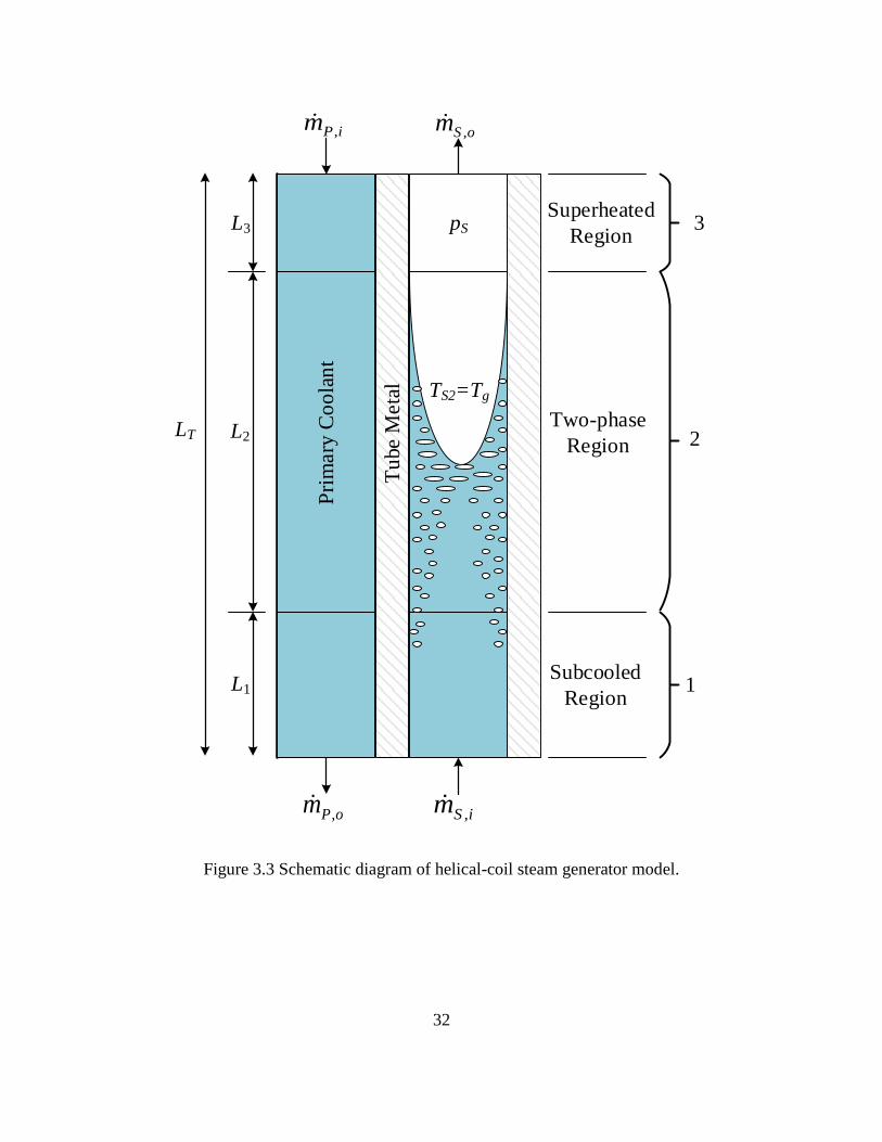
3.3.1 Governing equations and assumptions
The helical-coil steam generator model developed in this study is divided into
three regions according to conditions inside secondary side, i.e., subcooled, two-phase (or
boiling), and superheated. Control volumes are used to derive the model equations and
the length of each region is time-varying as depicted in Figure 3.3.
Page 46
32
L1
L2
L3 pS
iPm ,
oPm ,
TS2=Tg
iSm ,
oSm ,
Pri
mary
Co
ola
nt
Tu
be M
eta
l
Two-phase
Region
Subcooled
Region
Superheated
Region
LT
3
2
1
Figure 3.3 Schematic diagram of helical-coil steam generator model.
Page 47
33
The fundamental assumptions made to simplify the model development are listed
below:
Tubes inside the steam generator have identical flow. As such, a single tube heat
exchanger concept is used for simulating the dynamic behavior of the steam
generator.
One-dimensional fluid flow is utilized for both primary and secondary sides.
Perfect feedwater control is assumed, that is, feedwater and steam mass flow
rates are equal.
Heat conductivity along the axial direction is negligible.
Primary and secondary side pressures are assumed to be uniform.
The two-phase region is in thermal equilibrium.
He et al. [53] provide governing one-dimensional partial differential equations for
the conservation of mass and energy (Equations (3.24) and (3.25)) which are applicable
to all regions of the secondary side as well as an energy balance (Equation (3.26)) for the
tube metal
0
z
m
t
A SS
(3.24)
SMii
SSS TTdz
hm
t
pAhA
(3.25)
MPooMSiiM
MMp TTdTTdt
TAc
,
(3.26)
Page 48
34
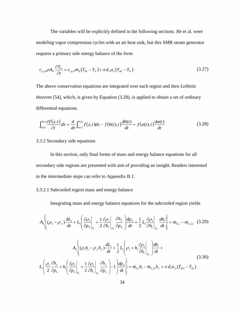
The variables will be explicitly defined in the following sections. He et al. were
modeling vapor compression cycles with an air heat sink, but this SMR steam generator
requires a primary side energy balance of the form
PMooPPiPPpP
PPp TTdTTmct
TAc
,, (3.27)
The above conservation equations are integrated over each region and then Leibnitz
theorem [54], which, is given by Equation (3.28), is applied to obtain a set of ordinary
differential equations.
)(
)(
)(
)(
)(),(
)(),(,
,tb
ta
tb
ta dt
tdattaf
dt
tdbttbfdztzf
dt
ddz
t
tzf (3.28)
3.3.2 Secondary side equations
In this section, only final forms of mass and energy balance equations for all
secondary side regions are presented with aim of providing an insight. Readers interested
in the intermediate steps can refer to Appendix B.1.
3.3.2.1 Subcooled region mass and energy balance
Integrating mass and energy balance equations for the subcooled region yields
12,,
1
11
1
111
11
2
1
2
1)(
1
SiSi
p
S
S
f
phS
fS mmdt
dh
hL
dt
dp
p
h
hpL
dt
dLA
SS
(3.29)
)(12
1
2
2
1)(
11112,,
1
111
11
1
1111
111
1
SMiifSiiS
S
S
f
phSS
f
i
p
ffS
TTdhmhmdt
dp
p
h
hph
p
hL
dt
dh
hhL
dt
dLhhA
S
S
(3.30)
Page 49
35
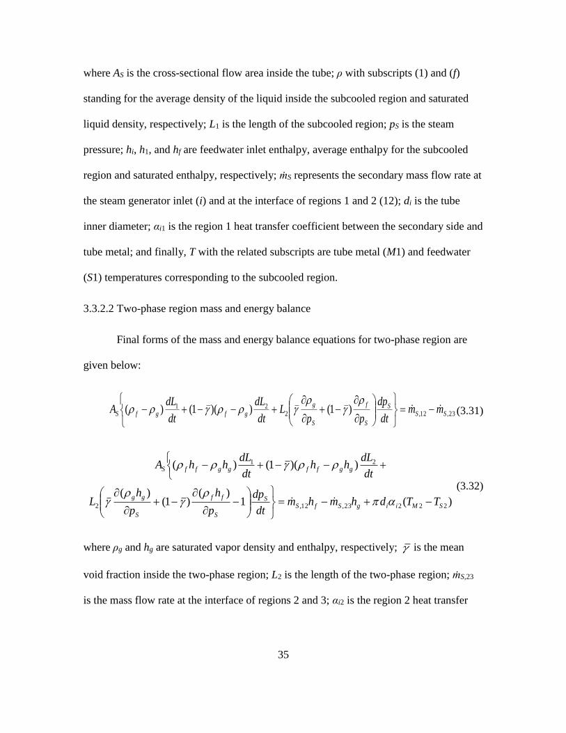
where AS is the cross-sectional flow area inside the tube; ρ with subscripts (1) and (f)
standing for the average density of the liquid inside the subcooled region and saturated
liquid density, respectively; L1 is the length of the subcooled region; pS is the steam
pressure; hi, h1, and hf are feedwater inlet enthalpy, average enthalpy for the subcooled
region and saturated enthalpy, respectively; ṁS represents the secondary mass flow rate at
the steam generator inlet (i) and at the interface of regions 1 and 2 (12); di is the tube
inner diameter; αi1 is the region 1 heat transfer coefficient between the secondary side and
tube metal; and finally, T with the related subscripts are tube metal (M1) and feedwater
(S1) temperatures corresponding to the subcooled region.
3.3.2.2 Two-phase region mass and energy balance
Final forms of the mass and energy balance equations for two-phase region are
given below:
23,12,221 )1())(1()( SS
S
S
f
S
g
gfgfS mmdt
dp
ppL
dt
dL
dt
dLA
(3.31)
)(1)(
)1()(
))(1()(
22223,12,2
21
SMiigSfSS
S
ff
S
gg
ggffggffS
TTdhmhmdt
dp
p
h
p
hL
dt
dLhh
dt
dLhhA
(3.32)
where ρg and hg are saturated vapor density and enthalpy, respectively; is the mean
void fraction inside the two-phase region; L2 is the length of the two-phase region; ṁS,23
is the mass flow rate at the interface of regions 2 and 3; αi2 is the region 2 heat transfer
Page 50
36
coefficient between secondary side and tube metal; TM2 is the tube metal temperature at
the two-phase region; and TS2 equals the saturation temperature (Tsat) at a given pressure.
3.3.2.3 Superheated region mass and energy balance
The same approach is followed for the superheated region and the resulting
equations for mass and energy balance are
oSSo
p
S
S
g
phS
gS mmdt
dh
hL
dt
dp
p
h
hpL
dt
LLdA
SS
,23,
3
33
3
333
213
2
1
2
1)()(
3
(3.33)
)(12
1
2
2
1)()(
333,23,
3
333
33
3
3333
2133
3
SMiiooSgSs
S
g
phSS
g
o
p
ggS
TTdhmhmdt
dp
p
h
hph
p
hL
dt
dh
hhL
dt
LLdhhA
S
S
(3.34)
where ρ3 is the average density of vapor inside the superheated region; L3 is the length of
the superheated region; ho and h3 are the steam outlet enthalpy and average enthalpy for
the superheated region; ṁS,o is the steam flow rate at the outlet of the steam generator; αi3
is the region 3 heat transfer coefficient between secondary side and tube metal; and T
with the related subscripts are tube metal (M3) and steam (S3) temperatures
corresponding to the superheated region.
3.3.3 Tube metal equations
An average temperature model, in which the temperature at each boundary is the
mean value of temperatures of adjacent wall regions, is utilized to observe the dynamics.
Page 51
37
Then the energy conservation equations corresponding to regions of the secondary side
are given by
)()()( 11111111
21,1
1, SMiiMPooMMMpMMM
MpMM TTdTTdLdt
dLTTcA
dt
dTLcA (3.35)
)()( 22222222
2, SMiiMPooM
MpMM TTdTTdLdt
dTLcA (3.36)
)()()(
)( 333333321
32,
3
3, SMiiMPooMMMpMM
M
MpMM TTdTTdLdt
LLdTTcA
dt
dTLcA
(3.37)
where AM, ρM, and cp,M are the cross-sectional area, density, and specific heat of the tube
metal, respectively; do is the outer diameter of the tube metal; αo represents the heat
transfer coefficient between the primary side and tube metal for each region; TP2 and TP3
are the average temperatures of the primary coolant for regions 2 and 3, respectively.
3.3.4 Primary side equations
In a similar manner, the energy balance equations for the primary side are
)()()( 111112,1
21,1
1, MPooPPPpPPPPpPPP
PpPP TTLdTTcmdt
dLTTcA
dt
dTLcA (3.38)
)()( 222223,2
2, MPooPPPpPP
PpPP TTLdTTcmdt
dTLcA (3.39)
)()()(
)( 33333,21
32,3
3, MPooPPiPpPPPPpPPP
PpPP TTLdTTcmdt
LLdTTcA
dt
dTLcA
(3.40)
where AP is the cross-sectional area of the primary coolant flow channel; ρP, cp,P, and ṁP
are the density, specific heat, and mass flow rate of the primary coolant; and TPi is the
primary coolant temperature at the steam generator inlet.
Page 52
38
3.3.5 Heat transfer coefficients and mean void fraction
In this study, the surface heat transfer coefficient for primary side is calculated by
utilizing the correlation for a bank of tubes given by [51]
6
25.0
36.0
102Re000,1
500Pr7.0
20
Pr
PrPrReNu
L
s
b
n
B
(3.41)
where Nu is the Nusselt number; coefficients B (0.021) and b (0.84) are determined from
a table in Reference [51] according to the configuration of tubes (aligned or staggered)
and the value of the Reynolds number; Prs is the Prandtl number at the surface
conditions; and nL is the number of tubes in the bank.
For the surface heat transfer coefficient of the secondary side, a modified version
of the Dittus-Boelter correlation [55], which is valid for single-phase heat convection, is
used
000,65Re000,6
PrRe023.0Nu
1.0
4.085.0
C
o
d
d
(3.42)
where dC is the coil diameter. The heat transfer coefficient for two-phase heat convection
is determined by taking advantage of the known variables at initial steady-state condition
for the two-phase region, i.e., the two-phase region length, the saturation temperature and
the temperatures of the tube metal, and the heat delivered by the primary side.
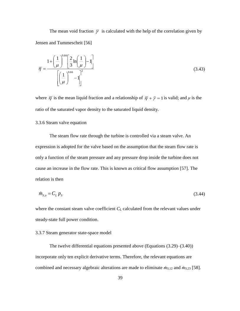
Page 53
39
The mean void fraction is calculated with the help of the correlation given by
Jensen and Tummescheit [56]
266.0
66.0
11
11
ln3
211
(3.43)
where is the mean liquid fraction and a relationship of 1 is valid; and μ is the
ratio of the saturated vapor density to the saturated liquid density.
3.3.6 Steam valve equation
The steam flow rate through the turbine is controlled via a steam valve. An
expression is adopted for the valve based on the assumption that the steam flow rate is
only a function of the steam pressure and any pressure drop inside the turbine does not
cause an increase in the flow rate. This is known as critical flow assumption [57]. The
relation is then
SLoS pCm , (3.44)
where the constant steam valve coefficient CL calculated from the relevant values under
steady-state full power condition.
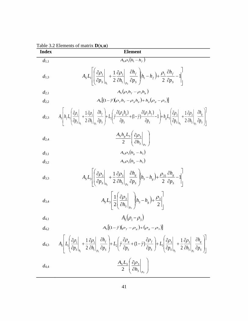
3.3.7 Steam generator state-space model
The twelve differential equations presented above (Equations (3.29)–(3.40))
incorporate only ten explicit derivative terms. Therefore, the relevant equations are
combined and necessary algebraic alterations are made to eliminate ṁS,12 and ṁS,23 [58].
Page 54
40
The resulting state vector is TPPPMMMoS TTTTTThpLL 32132121x
and the input vector TPPiioSiS mThmm ,,u . Then, it is possible to represent the
steam generator model in the following state-space form
uxfuxDx ,,1 (3.45)
where
10,102,101,10
9,9
8,81,8
7,72,71,7
6,6
5,51,5
4,43,42,41,4
4,33,32,31,3
4,23,22,21,2
3,11,1
0000000
000000000
00000000
0000000
000000000
00000000
000000
000000
000000
00000000
,
ddd
d
dd
ddd
d
dd
dddd
dddd
dddd
dd
uxD
)()(
)()(
)()(
)()(
)()(
)()(
)()(
)(
)()(
),(
33333,
222223,
111112,
3333333
2222222
1111111
,,
3333,
2222,,
1111,
MPooPPiPpP
MPooPPPpP
MPooPPPpP
SMiiMPoo
SMiiMPoo
SMiiMPoo
oSiS
SMiiogoS
SMiigoSfiS
SMiifiiS
TTLdTTcm
TTLdTTcm
TTLdTTcm
TTdTTdL
TTdTTdL
TTdTTdL
mm
TTLdhhm
TTLdhmhm
TTLdhhm
uxf
The elements of D(x,u) are in given in Table 3.2.
Page 55
41
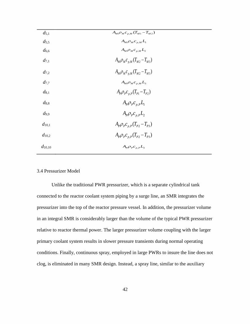
Table 3.2 Elements of matrix D(x,u)
Index Element
d1,1 fS hhA 11
d1,3
1
22
1 11
1
111
1S
f
f
S
f
phS
Sp
hhh
p
h
hpLA
S
d2,1 gfS hhA 31
d2,2 31 ggggffS hhhA
d2,3
S
g
phS
g
S
ff
S
gg
S
f
phS
fSp
h
hpLh
p
h
p
hL
p
h
hpLhA
SS3
3332
1
111
2
11
)()1(
)(
2
1
31
d2,4
Sp
gS
h
LhA
3
33
2
d3,1 33 hhA gS
d3,2 33 hhA gS
d3,3
1
22
1 313
3
333
3S
g
g
S
g
phS
Sp
hhh
p
h
hpLA
S
d3,4
22
1 33
3
33
g
p
S hhh
LA
S
d4,1 31 SA
d4,2 31 ggfSA
d4,3
S
g
phSS
f
S
g
S
f
phS
Sp
h
hpL
ppL
p
h
hpLA
SS3
3332
1
111
2
1)1(
2
1
31
d4,4
Sp
S
h
LA
3
33
2
Page 56
42
d5,1 )( 21, MMMpMM TTcA
d5,5 1, LcA MpMM
d6,6 2, LcA MpMM
d7,1 )( 32, MMMpMM TTcA
d7,2 )( 32, MMMpMM TTcA
d7,7 3, LcA MpMM
d8,1 )( 21, PPPpPP TTcA
d8,8 1, LcA PpPP
d9,9 2, LcA PpPP
d10,1 )( 32, PPPpPP TTcA
d10,2 )( 32, PPPpPP TTcA
d10,10 3, LcA PpPP
3.4 Pressurizer Model
Unlike the traditional PWR pressurizer, which is a separate cylindrical tank
connected to the reactor coolant system piping by a surge line, an SMR integrates the
pressurizer into the top of the reactor pressure vessel. In addition, the pressurizer volume
in an integral SMR is considerably larger than the volume of the typical PWR pressurizer
relative to reactor thermal power. The larger pressurizer volume coupling with the larger
primary coolant system results in slower pressure transients during normal operating
conditions. Finally, continuous spray, employed in large PWRs to insure the line does not
clog, is eliminated in many SMR design. Instead, a spray line, similar to the auxiliary
Page 57
43
spray in larger PWRs, is employed and designed to reduce the pressure when needed
[59].
The pressurizer model, as depicted in Figure 3.4, consists of two regions [34]: (1)
liquid, and (2) vapor. The following assumptions are carried out to simply the modelling:
Water-steam inside the pressurizer section is always at saturated conditions
corresponding to the primary coolant pressure.
Heat losses are neglected.
No condensation on the vessel wall or liquid surface.
Vapor Region (v)
Liquid Region (l)
Evaporation – condensation
Heater input, Qh
Spray flow ṁsp
ṁsu Surge flow
ṁec
Figure 3.4 Schematic diagram of pressurizer model.
Mass, energy, and volume balance equations for the pressurizer model are
presented as follows:
mass balances:
ecspsul mmm
dt
md (3.46)
Page 58
44
ec
v mdt
md (3.47)
For above equations, condensation occurs if ṁec < 0 while ṁec > 0 indicates that
evaporation takes place. In similar manner, ṁsu > 0 accounts for surge flow into the
pressurizer, whereas ṁsu < 0 means that the surge flow is out of the pressurizer.
volume balance:
gvflvlT mmVVV (3.48)
energy balances:
dt
dVphmhmhmQ
dt
dE lgecDRspsuh
l (3.49)
dt
dVphm
dt
dE vgec
v (3.50)
where ml and mv are the masses of the liquid and vapor in the pressurizer section; ṁ with
associated subscript gives surge flow (su), spray flow (sp), and evaporation-condensation
(ec) rates; VT represents the total volume of the pressurizer (constant) comprised of liquid
and vapor volumes; El and Ev denote energies of liquid and vapor; similarly, the products
of p(dV/dt) represent flow work of liquid and vapor; Qh is the heat given by electric
heaters; hDR is the primary coolant enthalpy in the downcomer region, and in the case of
insurge h = hHL (primary coolant enthalpy in the hot leg riser) otherwise h = hf (saturated
liquid enthalpy); and finally, hg is the saturated vapor enthalpy corresponding to primary
coolant pressure.
Page 59
45
Since saturated conditions are always assumed to be preserved inside the
pressurizer, it is possible to derive following equalities for temperature and pressure
satvl TTT (3.51)
satvlp pppp (3.52)
where the subscripts p, l, v, and sat stand for pressurizer, liquid, vapor, and saturation.
The pressurizer pressure is about 0.35 MPa less than the primary pressure due to the
difference in the elevation; see Figure 3.2. With the help of above equalities, the
pressurizer pressure equation is obtained after several algebraic manipulations.
)()()( fgecfDRspfsuh
p
f
P
f
l hmhhmhhmQdt
dp
p
hm
(3.53)
where hfg = hg − hf. Equation (3.48) is combined with an equation of state, in this case the
ideal gas law ( satvvP RTmVp ), to obtain an expression for the condensation-evaporation
rate which is
dt
dm
A
B
dt
dp
Am lp
ec 1
(3.54)
where
p
f
lp
p
satvv
sat
pmp
p
TRmV
RTA
p
f
lp
p
satvv
fp
pmp
p
TRmV
pB
Substituting Equations (3.46) and (3.53) into Equation (3.54) and applying
necessary alteration yields the final equation below for the pressurizer pressure.
Page 60
46
fgfDRspfgfsuh
pfgfg
f
P
f
l
hBA
Bhhmh
BA
BhhmQ
dt
dp
BA
h
A
B
A
h
p
hm
(3.55)
Finally, the summation of expansion (or contraction) of the water inside each
primary coolant section comprises the change in insurge (or outsurge) term [60] that is
n
i
iiisu
dt
TdVm
1
(3.56)
where Vi is the volume, Ti is the temperature, and ϑi is the slope of the primary coolant
density versus Ti for the i-th section.
3.5 Single SMR Unit model
The developed models are combined with a steam turbine representation, which
outputs the maximum attainable power Pm based on the steam properties, pressure and
enthalpy, and steam flow rate, to constitute a single SMR unit.
hmP oSTurbm , (3.57)
where ηTurb represents the turbine efficiency (0.83) [61]; and Δh is the steam enthalpy
difference between the turbine inlet and outlet.
The overall nonlinear system of coupled differential equations is introduced in the
form of a state-space model. The variables P, C, TF, TC1, TC2, THL, TDR, L1, L2, pS, ho, TM1,
TM2, TM3, TP1, TP2, TP3, pp are selected as the state variables, ρext, Qh, CL and TSi are
selected as the four input variables. The feedwater inlet temperature (TSi) is obtained from
the enthalpy hi. Then, the differential equations, Equations (3.1), (3.2), (3.4), (3.5), (3.6),
Page 61
47
(3.22), (3.23), (3.45), and (3.55), form the state equations. The combination of these state
equations with algebraic equations, Eqs. (3.20), (3.44), and (3.56), constitute the overall
reactor model.
The reactor model is implemented in MATLAB/Simulink [62], which is a user-
friendly graphical programming environment for modeling, simulation and analysis of
dynamic systems (see Figure 3.5).
Figure 3.5 Simulink representation of overall reactor model.
Page 62
48
3.6 Control Systems
3.6.1 Reactor control
The control of a reactor can be accomplished by three different modes in a PWR,
any one of which alters reactor thermal power in accordance with changes in certain
parameters, i.e., average primary coolant system temperature (Tavg), and steam pressure
(pS) [63].
3.6.1.1 Constant-average-temperature control mode
In this control mode, it is desired to keep the average temperature of the reactor
coolant system (RCS) constant regardless of the power output. In the case of an increase
in the load, the primary coolant average temperature decreases since the turbine extracts
more energy from the primary system. The control system, then, senses the change in the
RCS temperature and increases the system reactivity by withdrawing control rods. This
control mode is in compliance with the natural behavior of a reactor with negative
reactivity feedback coefficients and requires the least amount of control action.
The disadvantage of this program is that large variations in steam pressure and
temperature occur, assuming the steam valve position is fixed, which is not preferred by
the secondary system. However, it is preferred by the reactor since the constant-average-
temperature control mode minimizes required pressurizer size because the volume of the
water in the NSSS basically does not change. Figure 3.6 provides a depiction of this
control mode.
Page 63
49
Tem
per
ature
or
Pre
ssure
Hot Zero
PowerPower Output Full
Power
Thot
Tavg
Tcold
Tsteam
psteam
Figure 3.6 Characteristics of constant-average-temperature control model.
3.6.1.2 Constant-steam-pressure control mode
With this control mode, the reactivity of the reactor core is adjusted to maintain a
constant secondary pressure as the turbine load is changed. This control scheme causes a
rise in the temperature difference between primary and secondary sides by allowing the
average RCS temperature to increase in order to keep the steam pressure constant (see
Figure 3.7). The turbine favors the constant-steam-pressure control mode since excellent
steam conditions are provided. Furthermore, some problems associated with automatic
throttling devices and feedwater pumps are eliminated [64]. On the other hand, excessive
control rod motion is required and the hot leg temperature can approach the saturation
value corresponding to the primary coolant system pressure.
Page 64
50
Tem
per
ature
or
Pre
ssure
Hot Zero
PowerPower Output Full
Power
Thot
Tavg
Tcold
Tsteam
psteam
Figure 3.7 Characteristics of a constant-steam-pressure control mode.
3.6.1.3 Sliding-average-temperature control mode
For a slightly different mode from the aforementioned ones, the cold leg temperature
(or downcomer temperature) is kept constant which lets the average and hot leg temperatures
increase as the power output increases. The advantage of this program over the constant-
average-temperature program is that the change in the steam pressure according to the power
level is diminished. This program is also termed as a compromise program or non-constant
program since it is intended to provide a balance between the needs of the primary and
secondary systems. The relationship between temperatures and steam pressure for this control
mode is illustrated in Figure 3.8 [65].
Page 65
51
Hot Zero
PowerPower Output Full
Power
Thot
Tavg
Tcold
Tsteam
psteamTem
per
ature
or
Pre
ssure
Figure 3.8 Characteristics of a sliding-average-temperature control mode.
As a final note, most large PWRs utilizes a sliding-average-temperature program [66]
and for this reason, the same approach is adopted in this study. The control action in this
mode is achieved by a proportional-integral (PI) transfer function which takes the mismatch
between the setpoint and actual value of the cold leg temperature as the input and produces a
positive or negative external reactivity depending on the polarity and magnitude of the
mismatch, see Figure 3.9 and Equation (3.58).
Σ +
_
Reactivity
(Control rod motion)
PI
Controller
TDR,ref
TDR
Figure 3.9 Block diagram of sliding-average-temperature controller.
Page 66
52
refDRDR
TI
TPext TTs
KK ,
,
,
(3.58)
where TDR,ref is the reference value of the downcomer temperature; KP,T and KI,T are the
proportional and integral gain, respectively.
3.6.2 Primary coolant system pressure control
The control of the primary coolant system pressure is achieved by a bank of
heaters which compensate steady-state heat losses from the pressurizer and also regulate
the pressure under normal operating conditions. If the pressure is low, more power is
applied to the heaters to increase the pressure, and in the case of high pressure, the power
input to the heaters is decreased accordingly. When the pressure is below the control
range, then, additional (auxiliary) heaters are turned on. For the reverse situation in which
the pressure is too high and decreasing the heater power level is not sufficient, a spray
flow from the chemical and volume control system provides cooling and reduces the
pressure.
The controller model used in this study is a proportional-integral-derivative (PID)
controller given by Figure 3.10 and Equation (3.59) and only acts on the normally
operated heaters to keep the reactor coolant pressure constant.
Σ +
_
Heater
Output
PID
Controller
pP,ref
pP
Figure 3.10 Block diagram of pressurizer pressure controller.
Page 67
53
refPPpD
pI
pPh ppsKs
KKQ ,,
,
,
(3.59)
where pP,ref is the reference value of the primary coolant system pressure; KP,p, KI,p, and
KD,p are the proportional, integral and derivative gain, respectively.
Page 68
54
CHAPTER 4 TESTING THE DYMAMIC MODELS IN MATLAB/SIMULINK
In this chapter, the mathematical models discussed in the previous chapter are
tested and evaluated with the help of Matlab/Simulink v8.5 by applying common
disturbances to them. First, the dynamic simulation results for isolated core, steam
generator, and pressurizer models are presented, and then the response of the combination
of these models with hot leg riser and downcomer which constitute the single SMR unit
is presented.
4.1 Isolated Reactor Core Model
In order to test the isolated core model, small perturbations to reactivity and core
inlet coolant temperature are applied separately, and changes in the reactor thermal
power, core fuel and coolant temperatures, primary coolant flow rate and system
reactivity are demonstrated in Figures 4.1-4.6. The obtained results are compared to the
results from References [33].
Page 69
55
Figure 4.1 Reactor power (P) response to a step increase in the input variable for isolated
reactor core model.
Figure 4.2 Fuel temperature (TF) response to a step increase in the input variable for
isolated reactor core model.
Page 70
56
Figure 4.3 Reactor core coolant node 1 temperature (TC1) response to a step increase in
the input variable for isolated reactor core model.
Figure 4.4 Reactor core coolant node 2 temperature (TC2) response to a step increase in
the input variable for isolated reactor core model.
Page 71
57
Figure 4.5 Primary coolant mass flow rate (ṁC) response to a step increase in the input
variable for isolated reactor core model.
Figure 4.6 System reactivity (ρ) response to a step increase in the input variable for
isolated reactor core model.
Page 72
58
4.1.1 Response to a step change in external reactivity
A 7×10⁻⁵ (i.e., 1¢) increase in the reactivity due to control rod withdrawal is
applied to the system at t = 20 s. This action causes an increase in the fission rate and
neutron flux and, correspondingly, an initial rise in reactor thermal power, as shown in
Figure 4.1. Following the increased power generation, the fuel temperature increases and
more heat is transferred from the fuel region to the primary coolant in the core. The new
steady-state fuel (TF), coolant node 1 (TC1) and 2 (TC2) temperatures rise by 1.9 °C, 0.11
°C, and 0.22 °C, respectively, as shown in Figures. 4.2, 4.3 and 4.4. These temperature
changes drive the negative reactivity feedback mechanisms thereby resulting in the new
stable power level (P) of 161.2 MWt (see Figure 4.1). These results are consistent with
those from Reference [33] where a 7.1¢ step change in external reactivity was applied to
the linearized isolated core model developed for the H. B. Robinson Nuclear Plant. That
study shows the responses of the reactor thermal power and reactor outlet temperature
and their responses are identical with Figures 4.1 and 4.4 in terms of patterns of dynamic
behavior.
The coolant mass flow rate exhibits a pattern similar to coolant temperature which
is consistent with the theory since it is a function of temperature difference across the
core. The increase in coolant temperature induces an increase in the flow rate (ṁC) as
expected based on Equation (3.19) and it reaches a value of 709.6 kg/s at the new steady-
state operating point as shown in Figure 4.5. In addition, as the transient is caused by a
step change in external reactivity, a jump in system reactivity with a value of 7×10⁻⁵ is
observed. After that, it starts to decrease due to negative temperature coefficients of the
Page 73
59
fuel and coolant. When the new equilibrium is achieved, ρ goes to zero as it should be in
Figure 4.6.
4.1.2 Response to a step change in primary coolant inlet temperature
As the second transient, a 2.45 ºC (i.e., 1%) increase in the core inlet coolant
temperature is applied to the system, again, at t = 20 s. Due to this perturbation, the core
coolant node 1 and 2 temperatures increase (see Figures 4.3 and 4.4). Correspondingly,
the reactivity decreases due to the negative temperature coefficient of the moderator,
which leads to a sharp decrease in the reactor thermal power as seen in Figure 4.1. As a
result, the fuel temperature falls, and the heat transfer from fuel to coolant region
decreases, and the increase in the coolant temperatures stops. When a new stable point is
reached, the difference in the core thermal power compared to the initial condition is -8.2
MW as depicted in Figure 4.1. The average fuel temperature dips to 493.5 °C while the
rises in the core coolant node 1 and 2 temperatures becomes stable around values of
291.9 °C and 270.2 °C, respectively.
A sudden decrease in the coolant flow rate is observed as shown in Figure 4.5
since an increase in core coolant temperature is implemented. Following that, it starts to
recover as the coolant node 1 and 2 temperatures rise. However, the new steady-state
value, which is 695.6 kg/s, is less than its initial value of 708 kg/s because the reactor
operates with a lower thermal power output. Furthermore, the system produces negative
reactivity as depicted in Figure 4.6 although there is no change in control rod position.
This negative reactivity, an expected result of negative temperature coefficients, is due to
Page 74
60
initial rises in coolant temperatures. The negative reactivity is eventually canceled by
both the moderator and fuel temperature feedback coefficients.
4.2 Isolated Steam Generator Model
Testing the isolated nonlinear steam generator model is achieved by introducing
positive step disturbances to temperature of the primary coolant at the steam generator
inlet, primary coolant flow rate, feedwater inlet temperature and to steam valve position,
individually. Hence, there are two perturbations to the primary and two to the secondary
side. A comparison is made between results from the isolated steam generator and
References [41], [43], and [56]. Figures 4.7-4.11 show the behavior of some of the state
variables and the relevant discussion is provided afterwards.
Figure 4.7 Subcooled region length (L1) response to a step increase in the input variable
for isolated steam generator model.
Page 75
61
Figure 4.8 Two-phase region length (L2) response to a step increase in the input variable
for isolated steam generator model.
Figure 4.9 Superheated region length (L3) response to a step increase in the input variable
for isolated steam generator model.
Page 76
62
Figure 4.10 Steam pressure (pS) response to a step increase in the input variable for
isolated steam generator model.
Figure 4.11 Primary coolant outlet temperature (TP1) response to a step increase in the
input variable for isolated steam generator model.
Page 77
63
4.2.1 Response to a step change in primary coolant inlet temperature
For the first case, an increase of 2.9 °C (i.e., 1%) in the temperature of the
primary coolant at the steam generator inlet is introduced at t = 20 sec. The change in the
primary coolant temperature results in more heat transfer from the primary side to the
secondary via tube metal walls. Since the steam generator considered in this study is a
counter-flow heat exchanger, the disturbance is first felt by the superheated region of the
secondary side. The increase in the heat transfer rate causes a rise in the steam production
and, therefore, an elongation occurs in the superheated region length (L3) as illustrated in
Figure 4.9. Concurrently, the steam pressure (pS) increases (constant steam valve
position) and levels out at a new steady-state value of 3.19 MPa (see Figure 4.10). Figure
4.8 shows that two-phase region (boiling) length (L2) has a declining trend throughout the
simulation because the latent heat of evaporation (hfg) decreases with an increase in the
corresponding saturation pressure. The subcooled region length (L1), however, exhibits
an expansion initially and then starts decreasing as depicted in Figure 4.7. This behavior
is a result of two different mechanisms acting on the subcooled region simultaneously. As
the pressure rises the saturated liquid enthalpy (hf) increases which explains the early
response of the subcooled region length. Following that the increased heat transfer from
the primary coolant starts to overcome the need of extra heat to reach the saturation point
which accounts for the latter response. In their study, Ray and Bowman [41] tested the
helical-coil once-through steam generator model under five different, independent
perturbations. One of the perturbations is a 5% step change in the primary coolant inlet
temperature. A comparison between the results shows that the dynamic behaviors of the
Page 78
64
lengths of each region of the steam generators are very similar: a length decrease in the
subcooled and two-phase regions, and an increased length in the superheated region.
Finally, a difference of around +2.5 °C is observed in the primary coolant
temperature leaving the steam generator (TP1) when a new equilibrium is achieved; see
Figure 4.11.
4.2.2 Response to a step change in primary coolant flow rate
A 7 kg/s (i.e., 1%) step increase in the primary coolant flow rate is applied to the
isolated steam generator model at t = 20 sec. Similar to the first case, this transient causes
an increased heat transfer from the primary side to secondary side. Thus, the superheated
region length expands whereas the lengths of subcooled and boiling regions diminish as
seen in Figures 4.7-4.9. The difference in the initial behavior of the subcooled region is
owed to a relatively small increase in the steam pressure compared to the previous case.
The overall response of the steam generator model, however, is qualitatively similar with
the response from the previous case except the fact that the system variables are
quantitatively less perturbed.
Another comparison with Reference [41], in which a 5% step increase in the
primary coolant flow applied to the steam generator model, shows that all three region
lengths exhibit similar transient responses. Furthermore, Ray and Bowman also found in
their study that primary coolant inlet temperature and primary coolant flow simulation
scenarios are qualitatively similar, however, the system variables are more perturbed in
the first scenario.
Page 79
65
4.2.3 Response to a step change in feedwater inlet temperature
A 1.5 °C (i.e., 1%) step increase in the feedwater inlet temperature is introduced
at t = 20 sec for third simulation case. This change reduces the difference between the
feedwater temperature and saturation temperature corresponding to the steam pressure. In
addition, the secondary coolant velocity increases due to the decrease in the density for a
constant coolant flow rate. Therefore, the subcooled region length shrinks as depicted in
Figure 4.7. Furthermore, a slight reduction is observed in the steam pressure (see Figure
4.10) since the higher velocity induces more pressure drop. The latent heat of
vaporization increases with a decrease in the pressure which explains the rise in the two-
phase region length as shown in Figure 4.8. The superheated region length, on the other
hand, exhibits a small decline compared to the initial steady-state value; see Figure 4.9.
Finally, the primary coolant outlet temperature increases as the heat transfer from the
primary side to the secondary side diminishes due to the perturbation.
Before moving into next section, a comparison is made with Li et al. [43], where a
helical-coil steam generator model with helium as coolant is developed. Li et al.
presented dynamic behaviors of the (i) steam pressure, (ii) subcooled, two-phase, and
superheated regions, and (iii) helium outlet temperature for a 5% step increase in the
feedwater temperature. All these mentioned system variables respond similarly to the
results herein except the superheated region which expands a very small amount. This
difference is likely due to fact that Li et al. include momentum balance into modeling and
the pressure drop in each section of the steam generator is different while this study
assumes a uniform secondary side pressure.
Page 80
66
4.2.4 Response to a step change in steam valve opening
A 1% increase in the steam demand is introduced to the system via a step change
in the steam valve position at t = 20 sec. The perturbation engenders a sudden drop in the
steam pressure as depicted in Figure 4.10. Concomitantly, the corresponding saturation
temperature decreases whereas the latent heat of vaporization increases. These changes
result in a decline in the subcooled and two-phase region lengths and an expansion in the
superheated region length (see Figures 4.7-4.9). The primary coolant delivers more heat
to the secondary side due to the increased temperature difference between both sides
caused by the need of additional heat for steam demand. This is the reason that the
primary coolant outlet temperatures reaches a new equilibrium value slightly lower than
the initial value; Figure 4.11.
This simulation case shows a similarity with the dynamic simulation in Reference
[56], in which a moving boundary heat exchanger model is tested under three consecutive
perturbations: (1) a 5% increase in the speed of primary coolant pump speed at t = 0 s, (2)
a 10% increase in the outer heat transfer coefficient at t = 30 s, and (3) a 10% increase in
the nozzle coefficient (or steam valve) at t = 60 s. The comparison of these results after t
= 60 s with the results above reveals that steam pressure, subcooled and superheated
region lengths show similar dynamic responses. However, the responses for two-phase
region lengths are different from each other; the two-phase region length in Reference
[56] increases while it exhibits a declining trend over the course of the simulation herein.
This difference can be explained by the fact that in Reference [56], the perturbations are
Page 81
67
not applied independently and hence, the first and second perturbations may have some
lingering effect when the last one is introduced to the system.
4.2.5 Comparison of results
Table 4.1 summarizes comparisons of the simulation results for the isolated steam
generator model developed in this study against other references. The agreement of the
results provides a basis for the validation of the model and allows it to be used as a part
of the complete SMR model.
Table 4.1 Comparison of results for isolated steam generator model without control
systems
Scenario
Response of Isolated Steam
Generator Model
Other References
A step
increase in
primary
coolant
temperature
For a 1% change, a decrease in
the subcooled and two-phase
region lengths, and an increase
in the superheated region length
are observed.
In Reference [41], the dynamic
response of the lengths of each
region of the steam generators for
5% step change exhibit very similar
behavior.
A step increase
in primary
coolant flow
rate
The steam generator response is
qualitatively similar with the
response from the previous case
except the fact that the system
variables are quantitatively less
perturbed.
It is also found in Reference [41]
that the simulation results show a
similar pattern with less deviation
in system variables from initial
equilibrium conditions.
A step increase
in feedwater
inlet
temperature
A decline in the lengths of
subcooled and superheated
regions and an elongation in
two-phase region length are
observed for 1% step change. In
For a 5% increase, system variables
in Reference [43] respond similarly
except the superheated region
which expands a very small
amount. This difference is likely
Page 82
68
addition, a slight reduction in
the steam pressure occurs, and
the primary coolant outlet
temperature increases as the
heat transfer from the primary
side to the secondary side
diminishes.
due to fact that they include
momentum balance into modeling
and the pressure drop in each
section of the steam generator is
different.
A step increase
in steam valve
opening
Steam pressure decreases for a
1% increase in the valve
opening. The subcooled and
two-phase regions shrink, and
superheated region length
increases for this perturbation.
In Reference [56], steam pressure,
subcooled and superheated region
lengths show similar dynamic
responses. However, the response
for two-phase region length is
different which might be due to the
fact that the perturbations are not
applied independently and hence,
the first and second perturbations
may have some lingering effect
when the last one is introduced.
4.3 Isolated Pressurizer Model
The isolated pressurizer model has three inputs: (1) electric heater, (2) insurge (or
outsurge) flow, and (3) spray flow. The model is tested by perturbing the input variable
under investigation from its initial equilibrium value while keeping the others constant.
Figure 4.12 shows the response of the pressurizer pressure for changes in aforementioned
input variables. The pressure response is also compared with the response from
Reference [34].
Page 83
69
Figure 4.12 Pressurizer pressure (pp) response to a step increase in the input variable for
isolated pressurizer model without control system.
4.3.1 Response to a step change in electric heater input
A 100 kW step increase in the electric heater is applied to the isolated pressurizer
model between t = 20 sec and t = 120 sec. As the pressurizer is under saturated conditions
at the steady-state, vaporization starts because of the additional heat provided by the
heaters. That is the reason that the pressurizer pressure increases during the time of
disturbance as seen in Figure 4.12. After the electric heater is turned off, the pressure
stays at that level which is 0.12 MPa higher that the initial equilibrium value. This result
is congruent with the result from Reference [34], where a 100 kW step increase in the
electric heat input is applied to the linearized pressurizer model.
Page 84
70
4.3.2 Response to a step change in insurge flow rate
A 2 kg/s step increase in the surge flow (insurge) is introduced between t = 20 sec
and t = 120 sec. The liquid inside the pressurizer and the subcooled liquid from the
primary coolant system constitute a mixture that has a temperature lower than the
saturation temperature. The decrease in the temperature causes the contraction of the
liquid volume inside the pressurizer which accounts for the small gradual decrease in the
pressure; see Figure 4.12. When this result is compared with the same perturbation case
with a different magnitude in Reference [34], the dynamic responses do not agree each
other. This is most likely due to the fact that the coefficient of the surge term for the
linearized pressurized model in [34] is calculated by using only saturated liquid enthalpy
(h = hf). In this study, however, enthalpy term (h) in Equation (3.49) changes depending
on whether the surge flow is an insurge or outsurge flow.
4.3.3 Response to a step change in outsurge flow rate
As the third case, an outsurge flow perturbation of 2 kg/s is applied at t = 20 sec
and then the flow rate is reverted to its initial steady-state value at t = 120 sec. This
perturbation causes a decline in the liquid volume inside the pressurizer. Hence, the
pressurizer pressure shows a decreasing trend in Figure 4.12 and the overall pressure drop
is bigger compared to the result from the preceding case as expected.
4.3.4 Response to a step change in spray flow rate
For the last case, a 2 kg/s positive step change in the spray flow is introduced into
system between t = 20 sec and t = 120 sec. The temperature of the spray is lower than the
temperature of the insurge flow from the previous case. Due to this fact, the liquid
Page 85
71
mixture has a lower temperature compared to the mixture from the last case. This, then,
theoretically implies that the pressure drop should be larger for this transient which is
congruent with the pressure response as illustrated in Figure 4.12. The result from
Reference [34], again, for the same disturbance but with a different magnitude, exhibits
the same dynamic behavior with the result of the simulation case above.
As seen from the results for four different scenarios, only the increase in the
electric heater input induces a rise in the pressurizer pressure, which may explain why no
continuous spray exists in SMRs as stated earlier in Section 3.4.
4.3.5 Comparison of results
Table 4.2 summarizes comparisons of the simulation results for the isolated
pressurizer model developed in this study against a MS thesis by Thakkar [34]. The
agreement of the results provides a basis for the validation of the model and allows it to
be used as a part of the complete SMR model.
Table 4.2 Comparison of results for isolated pressurizer model without control systems
Scenario
Response of Isolated
Pressurizer Model
Other Reference
A 100 kW
step increase
in electric
heater
As the pressurizer is under
saturated conditions at the
steady-state, vaporization
starts because of the additional
heat provided by the heaters
and the pressurizer pressure
increases.
The model result is congruent with
the result from Reference [34],
where a 100 kW step increase in the
electric heat input is applied to the
linearized pressurizer model.
Page 86
72
A step
increase in
insurge flow
rate
A 2 kg/s step increase in the
surge flow (insurge) causes a
small gradual decrease in the
pressure.
The pressurizer response for a 50
lb/s step increase in Reference [34]
does not agree with the result herein
both qualitatively and quantitatively.
This is most likely due to the fact
that the coefficient of the surge term
for the linearized pressurized model
in [34] is calculated by using only
saturated liquid enthalpy (h = hf).
A step
increase in
spray flow
rate
A 2 kg/s positive step change
in the spray flow leads to a
drop in the pressurizer
pressure.
The result from Reference [34] for
the same disturbance but with a
different magnitude (50 lb/s),
exhibits the same dynamic behavior
with the result of the simulation case
above.
4.4 Single SMR Unit Model
4.4.1 Steady-state performance of the model
The overall SMR model is first simulated under steady-state conditions at 100%
power using Simulink. Some important simulation results are listed in Table 4.3, and the
steady-state temperature profile of the steam generator is shown in Figure 4.13. A
comparison of the results with the design data [28] and [30] shows that they are
consistent with each other, which justifies further studying of the model under dynamic
conditions. However, as no other researchers have published a complete SMR dynamic
Page 87
73
model, there will be no comparisons to make other than checking congruence of the
model response with theory.
Table 4.3 Steady-state values of important parameters
Parameter Value
Reactor thermal power 160.1 MW
Net electrical output 45.3 MW
Pressurizer pressure 12.41 MPa
Primary coolant mass flow rate 708 kg/s
Hot leg riser temperature 291 °C
Downcomer region temperature 246 °C
Steam generator total tube length 22.25 m
Subcooled region length 2.90 m
Two-phase region length 17.60 m
Superheated region length 1.75 m
Feedwater temperature 148.5 °C
Steam temperature 264 °C
Steam pressure 3.1 MPa
Steam mass flow rate 71.25 kg/s
It is noteworthy that the primary and secondary pressure values for the NuScale
SMR are considerably less than those for today’s large PWRs. Typical values for a
central station PWR are around 15.5 MPa and 7 MPa for the primary and secondary,
respectively.
Page 88
74
Figure 4.13 Steam generator temperature profile at steady-state (100% power).
4.4.2 Dynamic performance of the model
For the dynamic performance of the system, a step increase in each input variable,
i.e., control rod position (withdrawal), steam demand, pressurizer electric heat, and
feedwater temperature, is applied independently after 20 s of steady-state operation to
demonstrate that the simulation starts from a stable point and so that the initial steady-
state conditions can be seen clearly. The output of the electric heaters, however, reverts to
its initial steady-state value at the simulation time of 120 s.
Figures 4.14-4.26 exhibit responses of the different output variables for the
aforementioned perturbations. For each case, the input variable under investigation is
perturbed from its initial steady-state value while the others are kept constant. The results
are discussed in the following subsections according to the input step change.
Page 89
75
Figure 4.14 Reactor power (P) response to a step increase in the input variable for single
SMR unit.
Figure 4.15 Fuel temperature (TF) response to a step increase in the input variable for
single SMR unit.
Page 90
76
Figure 4.16 Reactor core coolant node 1 temperature (TC1) response to a step increase in
the input variable for single SMR unit.
Figure 4.17 Reactor core coolant node 2 temperature (TC2) response to a step increase in
the input variable for single SMR unit.
Page 91
77
Figure 4.18 Primary coolant mass flow rate (ṁC) response to a step increase in the input
variable for single SMR unit.
Figure 4.19 System reactivity (ρ) response to a step increase in the input variable for
single SMR unit.
Page 92
78
Figure 4.20 Subcooled region length (L1) response to a step increase in the input variable
for single SMR unit.
Figure 4.21 Two-phase region length (L2) response to a step increase in the input variable
for single SMR unit.
Page 93
79
Figure 4.22 Superheated region length (L3) response to a step increase in the input
variable for single SMR unit.
Figure 4.23 Steam pressure (pS) response to a step increase in the input variable for single
SMR unit.
Page 94
80
Figure 4.24 Primary coolant temperature (TP1) response at the steam generator outlet to a
step increase in the input variable for single SMR unit.
Figure 4.25 Pressurizer pressure (pp) response to a step increase in the input variable for
single SMR unit.
Page 95
81
Figure 4.26 Maximum attainable power (Pm) response to a step increase in the input
variable for single SMR unit.
4.4.2.1 Response to a step change in external reactivity
A 3.5×10⁻⁴ (i.e., 5¢) step increase in the reactivity due to control rod withdrawal
is applied to the system at t = 20 s as seen in Figure 4.19. Since this perturbation causes a
reduction in neutron absorption inside the core region, an upsurge in the fission rate and
neutron flux occurs. Therefore, the reactor thermal power (P) exhibits an 8.3 MWt
prompt jump as shown in Figure 4.14. Corresponding to the change in the thermal power,
the fuel temperature (TF) rises (Figure 4.15) which induces more heat transfer from the
fuel region to the primary coolant in the core. This is congruent with the increase in the
coolant node 1 (TC1) and 2 (TC2) temperatures as shown in Figures 4.16 and 4.17,
respectively.
Page 96
82
The increase in the temperature of the primary fluid at the steam generator inlet
leads to an increase in the heat transfer from the primary side to the secondary side of the
steam generator through the tube metal wall. More heat transfer raises the steam
generation and results in an expansion in the superheated region length (L3) as seen in
Figure 4.22. Concomitantly, the secondary pressure (pS) rises (see Figure 4.23) since no
change is made to the steam valve opening. As the pressure increases, the corresponding
saturation temperature of the secondary (feedwater) rises while the latent heat of
vaporization (hfg) declines which explains the decrease in the length of the two-phase
region (L2); see Figure 4.21. There is a competition between the increased heat delivery
and the need for more heat to bring the feedwater to the saturation point, and as Figure
4.20 reveals, there is a small decrease in the subcooled region length (L1) indicating that
the first mechanism dominates.
The overall increase in the temperature of the primary coolant system causes an
expansion of the coolant volume which, then, leads a surge flow into the pressurizer. The
mixture of the saturated liquid inside the pressurizer and the subcooled liquid from the
primary coolant system has a lower temperature than the saturation temperature
corresponding to the pressurizer pressure at the initial steady-state condition. This causes
a gradual decrease in the pressurizer pressure (pp) due to the perturbation in the control
rod position (see Figure 4.25).
All of these ensuing changes in the fuel and reactor coolant temperatures, and the
primary coolant pressure drive the reactivity feedback mechanisms thereby resulting in
the new stable power level of 161.4 MWt. The primary coolant mass flow rate (ṁc)
Page 97
83
shows a similar trend with the response of the reactor power as seen in Figures 4.14 and
4.18 and as expected from Equation (3.20). As the disturbance is initiated at the primary
side, the turbine starts to feel the associated effect after a time delay, which is
approximately 10 s and in agreement with the initial steady-state time constant for the hot
leg riser. The attainable power power (Pm) rises gradually and settles to a new steady-
state value of 45.7 MW as depicted in Figure 4.26. Finally, the system reactivity ρ returns
to zero, as it should, when the new equilibrium is achieved (Figure 4.19).
4.4.2.2 Response to a step change in feedwater inlet temperature
For the second scenario, a 7.425 °C (i.e., 5%) increase in the feedwater inlet
temperature (TSi) is introduced at t = 20 s. With this perturbation, the required heat for the
feedwater to reach the saturation temperature diminishes and the length of the subcooled
region is reduced as shown in Figure 4.20. In addition, the secondary fluid density
decreases which results in higher velocity, correspondingly. The increase in the fluid
velocity, then, engenders a larger pressure drop that accounts for the decline in the steam
pressure (see Figure 4.23). Thus, the latent heat of vaporization rises and an increase in
the length of the two-phase region is observed as depicted in Figure 4.21. Moreover, the
superheated region length levels out at a new equilibrium value shorter that the initial
one; see Figure 4.22.
This input perturbation raises the average secondary temperature such that there is
a decrease in the heat transfer from the primary side to secondary side. This causes a rise
in the temperature of the primary coolant at the steam generator outlet (TP1) as well as the
primary coolant temperature leaving the reactor core as seen in Figures 4.24 and 4.17,
Page 98
84
respectively. When the aforementioned temperature change is felt by the reactor core, the
system reactivity starts decreasing due to the negative reactivity temperature coefficients
and shows a dip with a minimum value of –1.78×10⁻⁵ as exhibited in Figure 4.19. Thus, a
reduction in both the reactor thermal power and fuel temperature is observed. At the new
steady-state operating level, the reactor thermal power has declined to 158.4 MW (Figure
4.14). In addition, the coolant flow rate also shows a similar pattern and decreases by
almost –2.6 kg/s. The attainable power power, however, exhibits a rise of about 0.2 MW
at the new steady-state condition since the additional heat content of the feedwater
exceeds the decrease in the reactor thermal power. This argument is supported by a
simple heat balance. Considering the steam generator as a boiler
boilerthm QnP (4.1)
hmQQQQ iSRXFWRXboiler , (4.2)
where nth is the Rankine cycle thermal efficiency (28%); δQ terms with subscripts (RX)
and (FW) are the change in heat provided by the reactor core (–1.6 MW) and feedwater,
respectively; Δh is the difference in the enthalpy of the feedwater before and after the
disturbance (32.6 kJ/kg) and the new equilibrium value of the feedwater flow rate (ṁS,i) is
70.8 kg/s. After the calculation is performed, δPm is 0.2 MW which agrees with the result
in Figure 4.26.
The pressurizer pressure, in this case, shows a very similar behavior compared to
the previous case and decreases due to the increase in the primary coolant temperature.
However, the pressure decrement is smaller since the increase in the temperature is less
compared to the first case.
Page 99
85
4.4.2.3 Response to a step change in pressurizer heater input
For the third case, a 100 kW increase in the pressurizer heater is applied to the
system, between t = 20 s and t = 120 s, so as to observe the effect of a disturbance
initiated inside the pressurizer on the primary and secondary sides. As more heat is
transferred to the saturated liquid inside the pressurizer, the pressurizer pressure starts to
increase until the heaters are turned off; see Figure 4.25. The deviation of the pressure
from the initial steady-state value causes a very small positive change in the reactor
thermal power due to the positive reactivity feedback coefficient of the primary pressure.
In similar manner, the fuel temperature also increases slightly. After the heaters are
turned off, the reactivity feedback mechanisms bring the system reactivity back to its
initial value. As understood from a careful examination of the plotted results, the reactor
remains at a slightly elevated temperature and pressure compared to the initial
equilibrium condition, but overall the disturbance does not have a significant impact on
the system state variables.
4.4.2.4 Response to a step change in steam valve opening
A 5% step increase in the steam valve opening is introduced at t = 20 s. The
action induces a sudden dip in the steam pressure, as depicted in Figure 4.23, as well as in
the corresponding saturation temperature. Thus, an abrupt vaporization takes place in the
steam generator, which is the underlying reason of the prompt jump in the apparent
attainable power; see Figure 4.26. This behavior is a result of the turbine model simply
calculating the attainable power as the product of associated variables used in the study.
In reality, however, the turbine inertia would prevent such response. The aforementioned
Page 100
86
momentary steam production cannot be maintained since the reactor core is not able to
respond to the need for steam instantly. These changes in the thermodynamic properties
lead to a decrease in the lengths of the subcooled and two-phase regions whereas an
elongation occurs in the superheated region length, as shown in Figures 4.20, 4.21, and
4.22, respectively.
The bigger temperature difference among the primary and secondary sides is due
to the increase in the steam demand causing more heat transfer to the secondary side from
the primary side and a decrease in the average temperature of the primary coolant.
Simultaneously, the coolant volume shrinks which results in a surge flow out of the
pressurizer. As a result, the primary coolant pressure in the pressurizer diminishes and
then settles down to a new equilibrium point; see Figure 4.25. The reactivity feedback
coefficients of the fuel and coolant temperatures and the primary pressure increase the
system reactivity, reaching a maximum value of 9×10⁻⁶, and drive the reactor thermal
power and fuel temperature up. The final steady-state value of the thermal power is
around 161.4 MW which corresponds to a new stable value of the attainable power of
45.7 MW.
4.5 Single SMR Unit Model with Control Systems
The effect of the control systems on the dynamic response of the single SMR unit
model is analyzed with two different scenarios:
1. Increase in steam valve opening, and
2. Increase in reactor thermal power.
Page 101
87
4.5.1 Increase in steam valve opening
For the first scenario, a 5% step increase in the load is applied to the system at t =
20 s, which results in a change in the steam valve opening. For comparison, two different
simulations under the same disturbance are run with and without the control systems.
Figures 4.27-4.33 exhibit the changes in the important state variables of the
system and the relevant discussion is provided afterwards.
Figure 4.27 Reactor power (P) response for a step increase in the load for single SMR
unit with and without control systems.
Page 102
88
Figure 4.28 Change in primary coolant temperatures for a step increase in the load for
single SMR unit without control systems.
Figure 4.29 Change in primary coolant temperatures for a step increase on the load for
single SMR unit with control systems.
Page 103
89
Figure 4.30 Pressurizer pressure (pP) response for a step increase in the load for single
SMR unit with and without control systems.
Figure 4.31 Steam pressure (pS) response for a step increase in the load for single SMR
unit with and without control systems.
Page 104
90
Figure 4.32 Maximum attainable power (Pm) response for a step increase in the load for
single SMR unit with and without control systems.
Figure 4.33 Change in thermal and maximum attainable power for a step increase in the
load for single SMR unit with control systems.
Page 105
91
When the disturbance is introduced without control systems, the steam pressure
decreases (see Figure 4.31) and flash steam is produced momentarily as explained
previously in Section 4.4.2.4. The rise in the steam demand causes more heat transfer
from the primary side to secondary. Thus, the primary coolant temperatures decrease as
shown in Figure 4.28 if no control action is taken. The reactivity feedback mechanisms
induce a positive reactivity into the system due to the reduction in the temperatures,
thereby leading to a gradual increase in the reactor thermal power (see Figure 4.27) even
though no adjustment to the control rod positions is made. However, the increase does
not satisfy the demand as the new steady-state value is around 166 MW, which is 3.5%
higher than the initial steady-state value but a reactor power of 8.2 MW is needed to meet
the demand. The attainable power also goes up by 1.7 MW and reaches a value of 47
MW accordingly, as depicted in Figure 4.32, at the new equilibrium operating point.
The decrease in the primary coolant temperatures reduces the coolant volume in
the primary loop and, therefore, an outsurge flow from the pressurizer via the baffle is
observed. As the liquid-vapor balance inside the pressurizer is lost, the pressure
diminishes with no active control on heaters until a new equilibrium is established (see
Figure 4.30).
If the same disturbance is applied while the control systems are active, the initial
decrease in the downcomer temperature (see Figure 4.29) produces an error signal for the
sliding-average-temperature controller. Following that the control rods are withdrawn
accordingly, thereby introducing a positive external reactivity. The external reactivity
results in a faster increase in the thermal power compared to the no-control case as shown
Page 106
92
in Figure 4.27. After an overshoot, the power level settles down to a value of 168.3 MW
which is congruent with the new setpoint established by the change in the load.
Furthermore, the downcomer temperature starts increasing, after the initial dip, and
reaches the pre-transient steady-state value (Figure 4.29), which is the desired behavior
achieved by the sliding-average-temperature controller. Finally, a small recovery is
noticed in the steam pressure with the reactor control as seen in Figure 4.31. These latter
observations are in agreement with the theory discussed in Section 3.6.1.3.
In a similar manner, the pressurizer pressure controller senses the difference
between the reference and actual values of the pressure after the transient is initiated, and
then applies more power to the heaters to keep the pressure constant. Figure 4.30 reveals
that around 60 s after the disturbance, the primary pressure is returned to its initial steady-
state value.
The attainable power rises in accordance with the thermal power and reaches a
value of 47.56 MW as desired in the control case (Figure 4.32). Figure 4.33 shows the
equilibrium deviation of the thermal (+8.2 MW) and attainable (+2.3 MW) power which
yields a thermal efficiency of 28%.
4.5.2 Increase in reactor thermal power
The other scenario to test the effectiveness of the control system is to increase (or
decrease) the reactor thermal power to a certain level within a desired time period when it
is necessary.
For this simulation case, the reference value of the sliding-average-temperature
controller is set to a new value of 253.3 °C , which was 245 °C initially, by a ramp
Page 107
93
function between t =20 s and t = 320 s. And the set point is kept at this new value for the
rest of the simulation (t > 320 s). A ramp is used instead of applying a step function to
avoid large power overshoot. This is congruent with the industry practice for PWRs [65].
This control action is intended to reach a new thermal power level of 5% higher than the
initial power level.
Figures 4.34-4.42 depict how some of the important system variables changes
over time for this simulation case.
Figure 4.34 Reactor power (P) response for a ramp increase in reactor power controller
reference value for single SMR unit.
Page 108
94
Figure 4.35 Fuel temperature (TF) response for a ramp increase in reactor power
controller reference value for single SMR unit.
Figure 4.36 Reactor core coolant node 2 temperature (TC2) response for a ramp increase
in reactor power controller reference value for single SMR unit.
Page 109
95
Figure 4.37 Primary coolant mass flow rate (ṁC) response for a ramp increase in reactor
power controller reference value for single SMR unit.
Figure 4.38 Normalized temperature difference (TC2/TC2,0 – TCi/TCi,0) for a ramp increase
in reactor power controller reference value for single SMR unit.
Page 110
96
Figure 4.39 System reactivity (ρ) response for a ramp increase in reactor power controller
reference value for single SMR unit.
Figure 4.40 Steam pressure (pS) response for a ramp increase in reactor power controller
reference value for single SMR unit.
Page 111
97
Figure 4.41 Pressurizer pressure (pp) response for a ramp increase in reactor power
controller reference value for single SMR unit.
Figure 4.42 Maximum attainable power (Pm) response for a ramp increase in reactor
power controller reference value for single SMR unit.
Page 112
98
As the controller reference value starts increasing, the difference between the
actual and reference values introduces an error signal to the controller which then causes
the movement of the control rods to induce a positive reactivity insertion (see Figure
4.39). Accordingly, the reactor thermal power and fuel temperatures show a rise as seen
in Figures 4.34 and 4.35. Following that the fuel-to-coolant heat transfer increases which
explains the increase in the reactor core coolant node 2 temperature in Figure 4.36.
Furthermore, the coolant mass flow rate exhibits an upward trend over the course of the
ramp increase and then a downward trend for the constant controller setpoint as seen in
Figure 4.37. This latter behavior is a result of the temperature difference in the primary
system (see Figure 4.38) which is the main driving mechanism for the coolant mass flow
rate as discussed in Section 3.1.2.3.3 by Equation (3.19).
With the increased temperature of the primary coolant, the temperature difference
between the primary and secondary sides of the steam generator expands, thereby
resulting in more heat transfer to the secondary side. The latter changes cause a growth in
the steam generation. Thus, steam pressure increases as shown in Figure 4.40. The
attainable power rises gradually and settles to a new steady-state value of 47.56 MW as
depicted in Figure 4.42 which is congruent with the new, desired operation conditions
discussed earlier.
The system reactivity exhibits a response similar to a square pulse shape (see
Figure 4.39). This is the result of external reactivity (control rods) and internal reactivity
(reactivity feedback mechanisms) acting together on the system. In other words, when the
disturbance is initiated, the external reactivity is dominant and the system reactivity
Page 113
99
increases. However, reactivity feedback mechanisms level off at a positive value after a
while. When the disturbance stops, since there is no external reactivity due to the control
rod movement, reactivity feedback mechanisms bring the system reactivity back to its
initial, pre-transient value. Finally, Figure 4.41 shows that this perturbation has minimal
impact on the pressurizer pressure.
Page 114
100
CHAPTER 5 CONCLUSIONS AND FUTURE WORK
5.1 Research Summary
Over the last decade, there has been a growing trend in the development and
commercialization of SMRs throughout the world. This interest is partially due to the
smaller initial capital investment required for SMRs compared to typical power reactors.
SMRs can be utilized to supply the electricity needs of remote areas with a lack of
transmission infrastructure. However, this is not the only option; water desalination,
general process heat for chemical or manufacturing processes, and district heating are
other possible applications that can make use of SMRs with minor design alterations.
With the integral type design of SMRs, generally the reactor vessel houses not
only the reactor core but also steam generators and pressurizer, and heat removal from
the reactor core is accomplished by natural circulation. This feature increases safety since
the primary coolant pumps, and associated failure modes are eliminated from the system.
The dynamic modeling of SMRs needs special attention and treatment due to
aforementioned unique features. That is the reason that, in this work, a detailed analytical
model for a passively cooled SMR is developed. The nuclear steam supply system
(NSSS) model includes representations for reactor core, steam generator, pressurizer, hot
leg riser and downcomer. The point kinetics equations with a single combined neutron
precursor group and the models for an overall heat transfer resistance and single-phase
natural circulation account for the neutronics and thermohydraulics in the reactor core
region, respectively. A lumped parameter, moving-boundary approach is adopted for the
once-through helical-coil heat exchanger in which boundaries between regions of
Page 115
101
different fluid states (i.e., subcooled, boiling, and superheated) can vary over time. For
the pressurizer model, an expression for the pressurizer pressure is derived from the
fundamental mass, volume and energy balances. Hot leg riser and downcomer are treated
as first-order lags. The NSSS model is incorporated with a turbine model which allows to
observe the attainable power with given steam flow, pressure, and enthalpy as input. The
overall nonlinear system is implemented in the Simulink dynamic environment. Various
simulation cases are run to test the capability of the developed model to predict the
dynamic response of the SMR. Finally, steady-state control programs for reactor power
and pressurizer pressure are also introduced. The obtained results and the relevant
discussion are presented.
5.2 Main Results of the Study
A nonlinear dynamic model for a passively cooled SMR is developed in this
study. Investigation into the components (i.e., reactor core, steam generator, and
pressurizer) of the model is carried out, separately, by applying perturbations to the input
parameters. Comparison between the obtained simulations results and the results from
References [33], [34], [41], [43], and [56] yields that the individual components of the
complete model are realistic, and able to predict the dynamic response. After the
validation, the combination of these models with hot leg riser and downcomer which
constitute the complete model for the single SMR unit is presented. Then, the single SMR
unit model is also tested by applying independent step changes into input variables.
Although there is no available data for the comparison since this is an original work, the
results are in good agreement with the theory.
Page 116
102
A sliding-average-temperature control mode is adopted and a PID controller is
used for reactor power and pressurizer pressure control, respectively. Dynamic
simulations show that proposed control schemes are able to keep the related state
variables at the desired values.
5.3 Future Work
The presented study can be extended in several directions. Possible areas in which
future work may be carried out include
A reduced order model for the linearized representation of the overall model can
be obtained to develop a model based controller.
The model developed in this study can be utilized for future studies where the
goal is an analysis and control of multiple SMRs coupled to a single steam
turbine−generator set.
Page 117
103
REFERENCES
[1] International Atomic Energy Agency, Advances in Small Modular Reactor
Technology Developments, p. 1, Sept. 2014.
[2] U.S. Department of Energy, Office of Nuclear Energy, Science and Technology,
The history of nuclear energy, DOE/NE-0088, p. 15, 2006.
[3] S. F. Burton, and A. G. Hosler, “Small Nuclear Power Plants, Volume One,
Design, Construction, and Operating Experience,” U. S. Atomic Energy
Commission, Tech. Rep. COO-284, Oct. 1966.
[4] World Nuclear Association, “Nuclear Power in the USA,” [Online]. Available:
http://www.world-nuclear.org/info/Country-Profiles/Countries-T-Z/USA--
Nuclear-Power/ [Accessed: 29 Sept. 2015].
[5] U.S. Nuclear Regulatory Commission (NRC), Information Digest, 2013-2014,
NUREG-1350, vol. 25, Aug. 2013.
[6] U.S. Energy Information Administration, Annual Energy Outlook 2018, U.S.
Department of Energy, DOE/EIA-0383, Jun. 2008.
[7] U.S. Department of Energy, Office of Nuclear Energy, “Small Modular Nuclear
Reactors,” [Online]. Available: http://energy.gov/ne/nuclear-reactor-
technologies/small-modular-nuclear-reactors [Accessed: 29 Sept. 2015].
[8] U.S. Department of Energy, Office of Nuclear Energy. “Energy Department
Announces New Investment in Innovative Small Modular Reactor,” [Online].
Available: http://energy.gov/articles/energy-department-announces-new-
investment-innovative-small-modular-reactor#! [Accessed: 29 Sept. 2015].
[9] Nuclear Energy Institute, “DOE Selects NuScale Power for SMR Development
Funds,” [Online]. Available: http://www.nei.org/News-Media/News/News-
Archives/DOE-Selects-NuScale-Power-for-SMR-Development-Fund [Accessed:
29 Sept. 2015].
[10] J. Vujić, R. M. Bergmann, R. Škoda, and M. Miletić, “Small modular reactors:
Simpler, safer, cheaper?,” Energy, vol. 45, pp. 288-295, Mar. 2012.
[11] D. T. Ingersoll, “Deliberately small reactors and the second nuclear era,”
Progress in Nuclear Energy, vol. 51, pp. 589-603, 2009.
[12] Locatelli G. SMR economics evaluation, The 4th Asia-Pacific forum on nuclear
technology: the small and medium reactors. Berkeley: UC; June 17-19, 2010.
Page 118
104
[13] World Nuclear Association, “Small Nuclear Power Reactors,” [Online].
Available: http://www.world-nuclear.org/info/Nuclear-Fuel-Cycle/Power-
Reactors/Small-Nuclear-Power-Reactors/#Note_f [Accessed: 29 Sept. 2015].
[14] R. Mazzi, "CAREM: an innovative-integrated PWR," in Proc. 18th International
Conference on Structural Mechanics in Reactor Technology (SMiRT-18), Beijing,
China, pp. 4407-4415, 2005.
[15] C. P. Marcel, F. M. Acuña, P. G. Zanocco, and D. F. Delmastro, "Stability of self-
pressurized, natural circulation, low thermo-dynamic quality, nuclear reactors:
The stability performance of the CAREM-25 reactor," Nuclear Engineering and
Design 265, pp. 232-243, 2013.
[16] H. Li, X. Huang, and L. Zhang, "A simplified mathematical dynamic model of the
HTR-10 high temperature gas-cooled reactor with control system design
purposes," Annals of Nuclear Energy 35, no. 9, pp. 1642-1651, 2008.
[17] Z. Wu, D. Lin, and D. Zhong, "The design features of the HTR-10," Nuclear
Engineering and Design 218, no. 1, pp. 25-32, 2002.
[18] K. M. Kim, B. I. Lee, H. H. Cho, J. S. Park, and Y. J. Chung, "Numerical study
on thermo-hydrodynamics in the reactor internals of SMART," Nuclear
Engineering and Design 241, no. 7, pp. 2536-2543, 2011.
[19] M. H. Chang, S. K. Sim, and D. J. Lee, "SMART behavior under over-
pressurizing accident conditions," Nuclear Engineering and Design 199, no. 1,
pp. 187-196, 2000.
[20] “B&W mPower Reactor Design Overview”, BW-JAH-2010-214, Babcock &
Wilcox Nuclear Energy, Lynchburg, Virginia, Jun. 2010.
[21] Z. Liu, and J. Fan, "Technology readiness assessment of small modular reactor
(SMR) designs," Progress in Nuclear Energy 70, pp. 20-28, 2014.
[22] J. A. Halfinger, and M. D. Haggerty, "The B&W mPower™ Scalable, Practical
Nuclear Reactor Design," Nuclear Technology 178, no. 2, pp. 164-169, 2011.
[23] R. J. Fetterman, A. W. Harkness, M. C. Smith, and C. Taylor, “An overview of
the Westinghouse small modular reactor,” in Proc. ASME 2011 Small Modular
Reactors Symposium, Washington, DC, USA, pp. 75-82.
[24] M. J., Memmott, A. W. Harkness, and J. Van Wyk, “Westinghouse Small
Modular Reactor nuclear steam supply system design,” in Proc. 2012
International Congress on Advances in Nuclear Power Plants, Chicago, IL, USA.
Page 119
105
[25] B. S. Triplett, E. P. Loewen, and B. J. Dooies, "PRISM: a competitive small
modular sodium-cooled reactor," Nuclear Technology 178, no. 2, pp. 186-200,
2012.
[26] A. Makhijani, "Light water designs of small modular reactors: facts and
analysis," Takoma Park: Institute for Energy and Environmental Research, 2013.
[27] J. N. Reyes Jr, and P. Lorenzini, "NuScale Power: A modular, scalable approach
to commercial nuclear power," Nuclear News 53, no. 7, pp. 97-104, 2010.
[28] “NuScale Plant Design Overview,” RP-1114-9375, Rev. 0, NuScale Power, LLC,
Corvallis, Oregon, Nov. 2014.
[29] International Atomic Energy Agency (IAEA), “NuScale Power Modular and
Scalable Reactor,” Advanced Reactor Information System database, [Online].
Available: https://aris.iaea.org/PDF/NuScale.pdf [Accessed: 2 Oct. 2015].
[30] “Trial Application of the Facility Safeguardibility Assessment Process to the
NuScale SMR Design,” DE-AC05-76RL01830, Rev 1, Pacific Northwest
National Laboratory, Jan. 2013.
[31] “Multi-Application Small Light Water Reactor Final Report,” INEEL/EXT-04-
01626, Idaho National Engineering and Environmental Laboratory, Idaho Falls,
Idaho, Dec. 2003.
[32] NuScale Power, “NuScale International Test Programs,” [Online]. Available:
http://www.nuscalepower.com/our-technology/test-programs/international-test-
programs [Accessed: 26 Oct. 2015].
[33] T. W. Kerlin, E. M. Katz, J. G. Thakkar, and J. E. Strange, “Theoretical and
experimental dynamic analysis of the H. B. Robinson nuclear plant,” Nuclear
Technology, vol. 30, pp. 299-316, Sept. 1976.
[34] J. G. Thakkar, “Correlation of theory and experiment for the dynamics of a
pressurized water reactor,” M.S. thesis, Dept. Nuc. Eng., Univ. Tennessee,
Knoxville, 1975.
[35] R. J. Onega, and K. E. Karcher, "Nonlinear dynamics of a pressurized water
reactor core," Nuclear Science and Engineering 61, no. 2, pp. 276-282, 1976.
[36] Y. Zvirin, "A review of natural circulation loops in pressurized water reactors and
other systems," Nuclear Engineering and Design 67, pp. 203-225, 1981.
[37] C. P. Marcel, H. F. Furci, D. F. Delmastro, and V. P. Masson, "Phenomenology
involved in self-pressurized, natural circulation, low thermo-dynamic quality,
nuclear reactors: The thermal–hydraulics of the CAREM-25 reactor," Nuclear
Engineering and Design 254, pp. 218-227, 2013.
Page 120
106
[38] B. Jang, M. H. Kim, and G. Jeun, "Experimental and computational investigation
of a natural circulation system in Regional Energy Reactor-10MW th," Nuclear
Engineering and Design 241, no. 6, pp. 2214-2223, 2011.
[39] A. Cammi, R. Ponciroli, A. B. di Tigliole, G. Magrotti, M. Prata, D. Chiesa, and
E. Previtali, "A zero dimensional model for simulation of TRIGA Mark II
dynamic response." Progress in Nuclear Energy 68, pp. 43-54, 2013.
[40] D. Chiesa, M. Clemenza, M. Nastasi, S. Pozzi, E. Previtali, G. Scionti, M. Sisti,
M. Prata, A. Salvini, and A. Cammi, "Measurement and simulation of the neutron
flux distribution in the TRIGA Mark II reactor core," Annals of Nuclear
Energy 85, pp. 925-936, 2015.
[41] A. Ray, and H. F. Bowman, "A nonlinear dynamic model of a once-through
subcritical steam generator," Journal of Dynamic Systems, Measurement, and
Control 98, no. 3, pp. 332-339, 1976.
[42] M. A. Abdalla, "A four-region, moving-boundary model of a once-through,
helical-coil steam generator," Annals of Nuclear Energy 21, no. 9, pp. 541-562,
1994.
[43] H. Li, X. Huang, and L. Zhang, "A lumped parameter dynamic model of the
helical coiled once-through steam generator with movable boundaries," Nuclear
Engineering and Design 238, no. 7, pp. 1657-1663, 2008.
[44] Z. Dong, "A Differential-Algebraic Model for the Once-Through Steam
Generator of MHTGR-Based Multimodular Nuclear Plants," Mathematical
Problems in Engineering, vol. 2015, pp. 1-12, 2015.
[45] K. E. Holbert, and N. Venkatesh, "Valid ranges for using the cross-power spectral
density phase angle for moderator temperature coefficient sign
determination," Nuclear Science and Engineering 119, no. 3, pp. 203-211, 1995.
[46] T. W. Kerlin, “Dynamic Analysis and Control of Pressurized Water Reactors,”
Control and Dynamic Systems, Advances in Theory and Applications, edited by
C.T. Leondes, Academic Press, vol. 14, 1978, pp. 103-212.
[47] J. J. Duderstadt, and L. J. Hamilton, Nuclear Reactor Analysis, New York: John
Wiley and Sons, Inc., 1976.
[48] “NuScale Codes and Methods Framework Description Report”, NP-TR-0812-
1682, Rev. 0, NuScale Power, LLC, Corvallis, Oregon, Jan. 2013.
[49] J. R. Lamarsh, and A. J. Baratta, Introduction to Nuclear Engineering, 3rd edition,
New Jersey: Prentice-Hall, 2001.
Page 121
107
[50] N. E. Todreas, and M. S. Kazimi, Nuclear Systems: Thermal Hydraulic
Fundamentals. vol. 1. CRC Press, 2011.
[51] T. L. Bergman, A. S. Lavine, F. P. Incropera, and D. P. Dewit, Fundamentals of
Heat and Mass Transfer. John Wiley & Sons, 2007.
[52] M. M. El-Wakil, Powerplant Technology, New York: McGraw-Hill, 2002. pp.
404-407.
[53] X. He, S. Liu, and H. Asada, "Modeling of vapor compression cycles for
advanced controls in HVAC systems," in Proc. American Control Conference,
Seattle, WA, USA, vol. 5, pp. 3664-3668, 1995.
[54] M. Willatzen, N. B. O. L. Pettit, and L. Ploug-Sørensen, "A general dynamic
simulation model for evaporators and condensers in refrigeration. Part I: moving-
boundary formulation of two-phase flows with heat exchange," International
Journal of Refrigeration 21, no. 5, pp. 398-403, 1998.
[55] L. Zhao, L. Guo, B. Bai, Y. Hou, and X. Zhang, "Convective boiling heat transfer
and two-phase flow characteristics inside a small horizontal helically coiled
tubing once-through steam generator," International Journal of Heat and Mass
Transfer 46, no. 25, pp. 4779-4788, 2003.
[56] J. M. Jensen, and H. Tummescheit, "Moving boundary models for dynamic
simulations of two-phase flows," in Proc. 2nd International Modelica Conference,
Oberpfaffenhofen, Germany, pp. 235-244, Mar. 2002.
[57] M. R. A. Ali, “Lumped parameter, state variable dynamic models for U-tube
circulation type nuclear steam generators,” Ph.D. dissertation, Dept. Nuc. Eng.,
Univ. Tennessee, Knoxville, 1976.
[58] B. P. Rasmussen, and A. G. Alleyne, “Dynamic modeling and advanced control
of air conditioning and refrigeration systems” Air Conditioning and Refrigeration
Center, College of Engineering. University of Illinois at Urbana-Champaign,
2006.
[59] R. J. Belles, “Key reactor system components in integral pressurized water
reactors (iPWRs),” Handbook of Small Modular Nuclear Reactors, edited by M.
D. Carelli, and D. T. Ingersoll, Woodhead Publishing, 2014, pp. 109-111.
[60] T. W. Kerlin, and E. M. Katz, "Pressurized water reactor modeling for long-term
power system dynamics simulation," Electric Power Research Institute (EPRI),
Palo Alto, CA, Tech. Rep. EL-3087, May 1983.
[61] U.S. Environmental Protection Agency (EPA), Combined Heat and Power
Partnership (CHP), Catalog of CHP Technologies, Mar. 2015.
Page 122
108
[62] Mathworks, “SIMULINK Dynamic System Simulation Language User’s Guide,”
2008.
[63] “Westhinghouse Technology Systems Manual Section 1.2,” [Online]. Available:
pbadupws.nrc.gov/docs/ML1122/ML11223A195.pdf [Accessed: 25 Feb. 2013].
[64] M. A. Schultz, Control of Nuclear Reactors and Power Plants, New York:
McGraw-Hill, 1955, pp. 128-179.
[65] L. E. Weaver, “Reactor Control,” Nuclear Power Safety, edited by J. H. Rust, and
L. E. Weaver, Pergamon Press, 1976, pp. 169-207.
[66] “Part 1: Introduction to Reactor Technology – PWR,” [Online]. Available:
http://pbadupws.nrc.gov/docs/ML1215/ML12159A222.pdf [Accessed: 25 Feb.
2016].
[67] Y. E. Kim, J. W. Park, and J. Cleveland, “Thermophysical properties database of
materials for light water and heavy water reactors,” International Atomic Energy
Agency, Vienna, Austria, Tech. Rep. IAEA-TECDOC-1496, Jun. 2006.
[68] S. E. Arda, "Implementing a Nuclear Power Plant Model for Evaluating Load-
Following Capability on a Small Grid," M.S. thesis, School of Elect., Comput.
and Energy Eng., Arizona State Univ., 2013.
[69] Mathworks, “X Steam, Thermodynamic properties of water and steam,” 2007.
[70] “Inconel alloy 690,” [Online]. Available:
http://www.specialmetals.com/assets/documents/alloys/inconel/inconel-alloy-
690.pdf [Accessed: 20 Oct. 2015].
Page 123
109
APPENDIX A
REACTOR CORE PARAMETERS AND CALCULATIONS
Page 124
110
A.1 Rector Core Parameters
Table A.1 Reactor core parameters
Variable Description Value Source
P Reactor thermal power 160 MWt Reference [29]
β Delayed neutron fraction 0.007 References [33], [45]
Λ Neutron generation time 20 μs References [33], [45]
λ Delayed neutron precursor decay
constant
0.1 s-1 References [33], [45]
αF Fuel temperature coefficient of
reactivity
–2.16×10⁻⁵/°C References [33], [45]
αC Coolant temperature coefficient of
reactivity
–1.8×10⁻⁴/°C References [33], [45]
αP Primary pressure coefficient of
reactivity
1.08×10⁻⁶/°C References [33], [45]
cp,F Specific heat of fuel 0.467 kJ/(kg·°C) Reference [67]
fd Fraction of power produced in fuel 0.975 Reference [68]
p Pin pitch 1.26 cm Reference [48]
d Fuel rod outside diameter 0.95 cm Reference [48]
H Active core height 2 m Reference [48]
nr Total number of rods 10693 Reference [48]
ρC Coolant density
(12.76 MPa and 268.3 °C)
780.3 kg/m3 Reference [69]
VC Coolant volume in core 1.879 m3 Calculated
mC Coolant mass in core 1466 kg Calculated
rf Fuel pellet radius 0.409 cm Reference [48]
nfr Total number of fuel rods 9768 Reference [48]
ρF Fuel density 10.96 g/cm3 Reference [67]
Page 125
111
mF Total fuel mass 11252 kg Calculated
hg Fuel gap heat transfer coefficient 5678 W/(m2·°C) Reference [49]
kf Fuel thermal conductivity 4.15 W/m·°C Reference [49]
kc Cladding thermal conductivity 19.04 W/m·°C Reference [49]
tg Gap thickness 0.057 cm Reference [48]
tc Cladding thickness 0.95 cm Reference [48]
De Equivalent diameter 1.178 cm Calculated
ṁC Coolant flow rate 708 kg/s Reference [30]
v Mean coolant velocity 0.966 m/s Calculated
μ Coolant dynamic viscosity
(12.76 MPa and 268.3 °C)
0.361 kg/(m·hr) Reference [69]
k Coolant thermal conductivity
(12.76 MPa and 268.3 °C)
0.598 W/(m·°C) Reference [69]
cp,C Specific heat of coolant
(12.76 MPa and 268.3 °C)
4.96 kJ/(kg·°C) Reference [69]
TC1 Average core coolant temperature 268.3 °C Reference [30]
hs Cladding surface heat transfer
coefficient
13730 W/(m2·°C) Calculated
AFC Effective heat transfer area 583 m2 Calculated
UFC Fuel-to-coolant heat transfer
coefficient
1135 W/(m2·°C) Calculated
TF Average fuel temperature 504 °C Calculated
Page 126
112
A.1.1 Coolant mass in reactor core
Figure A.1 shows the equivalent coolant channels in the reactor core for a square
fuel lattice. Based on this configuration, the calculation of the coolant flow in the core is
performed as follows:
dp
p
Fuel rods
Equivalent
channel
Figure A.1 Equivalent coolant channels in a square fuel lattice.
3222
2 m879.110693cm200)cm475.0()cm26.1(4
rC nH
dpV (A.1)
kg1466m
kg3.780m879.1
3
3 CCC Vm (A.2)
A.1.2 Fuel mass in reactor core
The mass of the fuel inside the core is calculated by
kg11252cm
g96.109768cm200)cm409.0(
3
22 FfrfF nHrm (A.3)
Page 127
113
A.1.3 Fuel-to-coolant heat transfer coefficient
The overall heat transfer resistance is defined in Section 3.1.2.2 as R = 1/(UA)FC
and Equation (3.9) gives an expression to calculate the heat transfer resistance. The only
unknown variable in that equation is the cladding surface heat transfer coefficient which
can be determined by Equation (3.10). However, the equivalent diameter (De) and the
Reynolds (Re) and Prandtl (Pr) numbers should be calculated.
cm178.1
)cm95.0(
)cm475.0()cm26.1(4
24
22
2
2
d
dp
De (A.4)
s
m966.0
kg1466
)m2()skg708( 1
C
C
m
Hmv
(A.5)
88548)hrmkg361.0(
)mkg3.780()sm966.0()cm178.1(Re
11
31
CevD (A.6)
8317.0)CmW598.0(
)hrmkg361.0()CkgkJ96.4(Pr
11
1111,
k
c Cp (A.7)
Replacing all parameters in Equation (3.10) with their values yields that
12-3/13.011
CmW137308317.088548cm178.1
)CmW598.0(0317.0
sh (A.8)
then by utilizing Equation (3.9), 1/R = 661705 W·°C-1. The effective heat transfer area
and fuel-to-coolant heat transfer coefficient can be calculated as
2m5839768)cm200()cm95.0( frFC nHdA (A.9)
Page 128
114
12-
2
1 CmW1135m583
1CW661705
1
FC
FCAR
U (A.10)
Finally, average fuel temperature can be found by Equation (3.7)
C504C3.268CW661705
1W10160975.0
1
6
1
CdF TPRfT (A.11)
Page 129
115
APPENDIX B
STEAM GENERATOR PARAMETERS AND CALCULATIONS
Page 130
116
B.1 Derivation of Secondary Side Equations
B.1.1 Subcooled region
Integration of the mass balance equation (Equation 3.24) over the subcooled
region yields that
011
00
z
z
mz
t
A LS
LS
(B.1)
1
10,12,
1 0L
iSSLSS mmdt
dLAdz
dt
dA (B.2)
where ρ(L1) is the saturated liquid density ρf. In addition, it is assumed that average
enthalpy and density of the liquid for the subcooled region equal h1 = 0.5(hi + hf) and
ρ1 = ρ(pS,h1), respectively.
The rate of change of mass in the liquid region, first term of Equation (B.2), can
be evaluated as:
1
0
11
1111 0
L
SSSSdt
dLA
dt
dLAL
dt
dAdz
dt
dA
(B.3)
then Equation (B.2) can be rewritten as:
12,,1
11
1 SiSfS mmdt
dL
dt
dLA
(B.4)
The time derivative of the average liquid density equals the following expression
by using the chain rule.
Page 131
117
dt
dh
hdt
dp
p
h
hp
hhdt
d
hdt
dp
p
dt
dh
hdt
dp
pdt
d
iS
S
f
hS
fiS
hS
S
hS
SS
S
S
1
1
1
11
1
11
1
1
111
2
1
2
1
2
1
1
1
1
(B.5)
Finally, inserting Equation (B.5) into Equation (B.4) gives the mass balance
equation for the subcooled region which is
12,,
1
11
1
111
11
2
1
2
1)(
1
SiSi
p
S
S
f
phS
fS mmdt
dh
hL
dt
dp
p
h
hpL
dt
dLA
SS
(B.6)
In a similar manner, integration of the energy balance equation (Equation 3.25)
over the subcooled region gives that
111
000
L
SMii
LS
LSS TTd
z
hm
t
pAhA
(B.7)
)()( 111,12,0
11
111 SMiiiiSfS
L
LLLSS TTdhmhmdt
dLphAdzph
dt
dA (B.8)
and evaluating the first term of Equation (B.8) results in
dt
dpL
dt
dLp
dt
dhL
dt
dhL
dt
dLhA
dt
dpL
dt
dLph
dt
dL
dt
dLhA
dt
dpLA
dt
dLpALh
dt
dALph
dt
dAdzph
dt
dA
SSS
SSS
SSSSSSS
L
S
111
111
111
11
11
1111
11
11
1111110
01
(B.9)
then, replacing the average liquid enthalpy and the rate of change of the average liquid
density in Equation (B.9) with their equivalences yields the equation below.
Page 132
118
dt
dh
dt
dhL
dt
dh
hdt
dp
p
h
hphLA
dt
dpL
dt
dLphAdzph
dt
dA
fiiS
S
f
hS
S
SSS
L
S
SS
11
1
1
1
1111
11
110
2
1
2
1
2
1
)(
1
1
(B.10)
Combining Equations (B.8) and (B.10) gives the energy balance equation for the
subcooled region.
)(
2
1
2
1
2
1
111,12,11
1
11
1
1
1
1111
111
1
SMiiiiSfSSSffSS
S
fiiS
S
f
hS
SS
TTdhmhmdt
dLpA
dt
dLhA
dt
dpLA
dt
dh
dt
dhL
dt
dh
hdt
dp
p
h
hphL
dt
dLphA
SS
(B.11)
After algebraic manipulations, the final form of the energy conservation equation
is obtained as:
)(12
1
2
2
1)(
11112,,
1
111
11
1
1111
111
1
SMiifSiiS
S
S
f
phSS
f
i
p
ffS
TTdhmhmdt
dp
p
h
hph
p
hL
dt
dh
hhL
dt
dLhhA
S
S
(B.12)
B.1.2 Two-phase region
The mass balance equation for the two-phase region is derived by integrating the
general mass balance equation over the region and, then, applying Leibnitz theorem.
021
1
21
1
zz
mz
t
A LL
L
SLL
L
S
(B.13)
21
1211
012,23,211
LL
LSSLLSLSS mm
dt
LLdA
dt
dLAdz
dt
dA (B.14)
Page 133
119
where ρ(L1+L2) is the saturated vapor density ρg.
The rate of change of mass in the two-phase region, first term of Equation (B.14),
can be evaluated as:
21
1
22
2221221
LL
LSSSS
dt
dLA
dt
dLALLL
dt
dAdz
dt
dA
(B.15)
where ρ2 is the two-phase region mean density and equals to fg 12 . Using
this equity, Equation (B.15) can be rewritten as:
21
1
122
2
LL
L
S
S
f
S
g
SSSdt
dp
ppLA
dt
dLAdz
dt
dA
(B.16)
and, the combination of Equations (3.14) and (3.16) gives the mass balance equation in
the form of
23,12,
2112
22 1
SS
gSgSfSS
S
f
S
g
SS
mm
dt
dLA
dt
dLA
dt
dLA
dt
dp
ppLA
dt
dLA
(B.17)
and, after substituting ρ2 with its equivalence result in the final form of the mass balance
equation for the two-phase region.
23,12,221 )1())(1()( SS
S
S
f
S
g
gfgfS mmdt
dp
ppL
dt
dL
dt
dLA
(B.18)
The same methodology is applied to the general energy balance equation in order
to obtain the energy conservation equation of the two-phase region.
21
1
21
1
21
1
LL
LSMii
LL
L
SLL
L
SS TTdz
hm
t
pAhA
(B.18)
Page 134
120
)(
)(
22212,23,
112
111
21
1121212
SMiifSgS
LLLS
LL
LLLLLLLSS
TTdhmhm
dt
dLphA
dt
LLdphAdzph
dt
dA
(B.19)
An expression can be obtained for the integral term of Equation (B.19) as follows:
dt
dpLA
dt
dLpA
dt
dLhhA
dt
dp
p
h
p
hLA
Lphhdt
dAdzph
dt
dA
SSSSffggS
S
S
ff
S
gg
S
SffggS
LL
LS
222
2
2
1
1
1)(21
1
(B.20)
where
S
g
g
S
g
g
S
gg
p
h
ph
p
h
, and
S
f
f
S
f
f
S
ff
p
h
ph
p
h
. The combination
of Equations (B.19) and (B.20) results in the energy balance equation.
)(
11
22212,23,
1212
2
22
SMiifSgS
SffSSggSS
SSS
ffggSS
S
ff
S
gg
S
TTdhmhm
dt
dLphA
dt
LLdphA
dt
dpLA
dt
dLpA
dt
dLhhA
dt
dp
p
h
p
hLA
(B.21)
After rearranging Equation (B.21), the final form of the energy balance equation
is
)(1)(
)1()(
))(1()(
22223,12,2
21
SMiigSfSS
S
ff
S
gg
ggffggffS
TTdhmhmdt
dp
p
h
p
hL
dt
dLhh
dt
dLhhA
(B.22)
Page 135
121
B.1.3 Superheated region
The mass balance equation for the superheated region is obtained after the
following steps:
02121
zz
mz
t
A L
LL
SL
LL
S
(B.23)
L
LLSoSLLSS mm
dt
LLdAdz
dt
dA
2121
023,,21 (B.24)
It is assumed that average enthalpy and density of the vapor for the superheated
region equal h3 = 0.5(ho + hg) and ρ3 = ρ(pS,h3), respectively.
The rate of change of mass in the superheated region, first term of Equation (B.2),
can be evaluated as:
L
LLSSSS
dt
dLA
dt
LLdALLL
dt
dAdz
dt
dA
21
33
213321
(B.25)
then Equation (B.24) can be rewritten as:
oSSggSS mm
dt
dLA
dt
dLA
dt
dLA ,23,
23
13
33
(B.26)
The time derivative of the average liquid density equals the following expression
by using the chain rule.
Page 136
122
dt
dh
hdt
dp
p
h
hp
hhdt
d
hdt
dp
p
dt
dh
hdt
dp
pdt
d
oS
S
g
hS
goS
hS
S
hS
SS
S
S
3
3
3
33
3
33
3
3
333
2
1
2
1
2
1
3
3
3
(B.27)
Finally, inserting Equation (B.27) into Equation (B.26) gives the mass balance
equation for the superheated region which is
oSSo
p
S
S
g
phS
gS mmdt
dh
hL
dt
dp
p
h
hpL
dt
LLdA
SS
,23,
3
33
3
333
213
2
1
2
1)()(
3
(B.28)
In a similar manner, integration of the energy balance equation (Equation 3.25)
over the superheated region gives that
L
LLSMii
L
LL
SL
LL
SS TTdz
hm
t
pAhA
212121
(B.29)
)( 333
23,,21
21212121
SMii
gSooS
L
LLLLLLLLSS
TTd
hmhmdt
LLdphAdzph
dt
dA
(B.30)
and evaluating the first term of Equation (B.30) results in
dt
dpL
dt
LLdp
dt
dhL
dt
dhL
dt
LLdhA
dt
dpL
dt
LLdph
dt
dL
dt
LLdhA
dt
dpLA
dt
dLpALh
dt
dALph
dt
dAdzph
dt
dA
SSS
SSS
SSSSSSS
L
LLS
3213
333
3321
33
321
33321
33
33
33333321
(B.31)
Page 137
123
then, replacing the average vapor enthalpy and the rate of change of the average vapor
density in Equation (B.31) with their equivalences yields the equation below.
dt
dh
dt
dhL
dt
dh
hdt
dp
p
h
hphLA
dt
dpL
dt
LLdphAdzph
dt
dA
gooS
S
g
hS
S
SSS
L
LLS
SS
33
3
3
3
33
33
321
33
2
1
2
1
2
1
3
21
(B.32)
Combining Equations (B.30) and (B.32) gives the energy balance equation for the
subcooled region.
)(
2
1
2
1
2
1
33323,,
2121333
3
3
3
3333
2133
3
SMiigSooS
SSggSS
S
goS
oS
S
g
hS
SS
TTdhmhm
dt
LLdpA
dt
LLdhA
dt
dpLA
dt
dh
dt
dhLA
dt
dh
hdt
dp
p
h
hphL
dt
LLdphA
SS
(B.33)
After algebraic manipulations, the final form of the energy conservation equation
is obtained as:
)(12
1
2
2
1)()(
333,23,
3
333
33
3
3333
2133
3
SMiiooSgSs
S
g
phSS
g
o
p
ggS
TTdhmhmdt
dp
p
h
hph
p
hL
dt
dh
hhL
dt
LLdhhA
S
S
(B.34)
Page 138
124
B.2 Steam Generator Parameters
Table B.1 Steam generator parameters at full power
Variable Description Value Source
L Steam generator tube length 22.25 m Reference [31]
L1 Subcooled region length 1.75 m Calculated
L2 Two-phase region length 17.6 m Calculated
L3 Superheated region length 2.9 m Calculated
do Tube outside diameter 1.6 cm Reference [31]
di Tube inner diameter 1.42 cm Reference [31]
St Transverse pitch 2.88 cm Reference [31]
Sl Longitudinal pitch 2.4 cm Reference [31]
N Total number of tubes 1012 Reference [31]
ṁS,o Steam flow rate 71.25 kg/s Reference [30]
pS Steam pressure 3.1 MPa Reference [30]
TSi Feedwater inlet temperature 149 °C Reference [30]
TSo Steam outlet temperature 264 °C Reference [30]
Apht Total tube outer heat transfer area 1123 m2 Calculated
Asht Total tube inner heat transfer area 1004.5 m2 Calculated
kt Thermal conductivity of Inconel
690 at 280 °C
16.92 W/(m·°C) Reference [70]
CL Steam valve coefficient 2.2983 kg/(s·bar) Calculated
Page 139
125
The steam generator heat transfer process involve three mechanisms: (1)
convective heat transfer between the primary coolant and the steam generator tube outer
surface, (2) conductive heat transfer within the steam generator tube metal, and (3)
convective heat transfer between the steam generator tube inner surface and the
secondary coolant. Equations (3.41) and (3.42) give the correlations to calculate heat
transfer coefficients for the first and third mechanisms. Reference [70], on the other hand,
provides thermal conductivity data of Inconel 690 to determine the conductive heat
transfer coefficient. Since the steam generator model consists of three regions, these
calculations should be performed for each region. The MATLAB code in the following
subsection describes the heat transfer in the steam generator and generates a plot showing
the steady-state temperature profile for the steam generator (see Figure 4.13)
B.2.1 MATLAB code for steam generator heat transfer calculations
%% Checking heat balance between primary and secondary
% Heat given by primary coolant
G_p = 708; % kg/s
P_p = 124.1; % bar
T_pi = 291.1; % C
T_po = 245.5; % C
h_pi = XSteam('h_pT',P_p,T_pi); % kJ/kg
h_po = XSteam('h_pT',P_p,T_po); % kJ/kg
Q_p = G_p*(h_pi - h_po)/1000; % MWt
% Heat picked up by secondary coolant
G_s = 71.25; % kg/s
P_s = 31; % bar
T_so = 263.8; % C
T_si = 148.9; % C
h_so = XSteam('h_pT',P_s,T_so); % kJ/kg
h_si = XSteam('h_pT',P_s,T_si); % kJ/kg
Q_s = G_s*(h_so - h_si)/1000; % MWt
%% Tp12 - Primary Coolant Temperature at Boundary of Region 1
h_s12 = XSteam('hL_p',P_s); %
Q_s1 = -(h_si - h_s12)*G_s; %
Q_p1 = Q_s1; %
c_p1= XSteam('Cp_pt',P_p,249);
T_p12 = Q_p1/(c_p1*G_p) + T_po;
%% Tp23 - Primary Coolant Temperature at Boundary of Region 2
Page 140
126
h_s23 = XSteam('hV_p',P_s);
Q_s2 = -(h_s12 -h_s23)*G_s; %
Q_p2 = Q_s2; %
c_p2= XSteam('Cp_pt',P_p,278);
T_p23 = Q_p2/(c_p2*G_p) + T_p12;
%% Tpi - Primary Coolant Temperature at Boundary of Region 3
Q_s3 = -(h_s23 -h_so)*G_s; %
Q_p3 = Q_s3; %
c_p3= XSteam('Cp_pt',P_p,290);
T_pi_cal = Q_p3/(c_p3*G_p) + T_p23;
%% Average Primary Coolant Temperature for Each Region
L_1 = 2.89; % subcooled section length (m)
L_2 = 17.6; % boiling section length (m)
L_3 = 1.76; % superheated section length (m)
T_p1 = (T_po + T_p12)/2;
T_p2 = (T_p12*(L_1+L_2) - T_p1*L_2)/L_1;
T_p3 = (T_p23*(L_2+L_3) - T_p2*L_3)/L_2;
%% SUBCOOLED REGION
%% Heat Transfer from Primary Coolant to Tube Outer Surface, Subcooled
do = 1.5875; % tube outside diameter (cm)
St = do*1.8; % transverse pitch (cm)
Sl = do*1.5; % longitudinal pitch (cm)
N = 1012; % total number of steam generator tubes
G_pc = G_p/N; % primary flow rate per channel (kg/s)
de = 4*((St*Sl - pi*(do/2)^2) / (pi*do)); % equivalent diameter (cm)
rho_p1 = XSteam('rho_pT',P_p,T_p1); % density of water (kg/m^3)
A_pc = St*Sl - pi*(do/2)^2; % primary coolant flow area per channel (cm^2)
V_pc1 = L_1*A_pc/10000; % primary coolant volume per channel (m^3)
m_p1 = V_pc1*rho_p1; % primary coolant mass per channel (kg)
v_p1 = (G_pc*L_1)/m_p1; % primary coolant velocity (m/s)
v_mp1 = (St/(St-do))*v_p1; % primary coolant max velocity (m/s)
mu_p1 = XSteam('my_pT',P_p,T_p1); % viscosity of water (kg/m-s)
k_p1 = 0.630075; % thermal conductivity of water (W/m-C)
Re_p1 = (0.01*do*v_mp1*rho_p1/mu_p1); % Reynolds number
Pr_p1 = 1000*c_p1*mu_p1/k_p1; % Prandtl number
Nu_p1 = 0.021*Re_p1^0.84*Pr_p1^0.36; % Nusselt number
H1 = (Nu_p1*k_p1/(do*0.01)); % heat transfer coefficient (W/m^2-C)
A_ph1 = (pi*do*L_1)/100; % heat transfer area per tube (m^2)
A_pht1 = N*A_ph1; % total heat transfer area (m^2)
T_m1o = T_p1 - (Q_p1/(H1*A_pht1))*1000; % tube metal outside temperature (C)
%% Heat Transfer from Tube Outer Surface to Tube Inner Surface, Subcooled
k_t1 = 16.16; % thermal conductivity of Inconel 690 at 240 C (W/m-C)
di = 1.42; % tube inner diameter (cm)
t = 0.09; % tube thickness (cm)
R_t1 = (1/(2*pi*k_t1*L_1))*log((di/2 + t)/(di/2)); % thermal resistance (W/C)^-1
H_t1 = 1/(R_t1*A_ph1); % heat transfer coefficient (W/m^2-C)
T_m1i = T_m1o - (Q_p1/(H_t1*A_pht1))*1000; % tube metal inside temperature (C)
%% Heat Transfer from Tube Inner Surface to Secondary Coolant, Subcooled
G_st = G_s/N; % secondary coolant flow per tube (kg/s)
rho_s1 = XSteam('rho_pT',P_s,194); % density of water(kg/m^3)
A_sc = pi*(di/2)^2/10000; % secondary coolant flow are per tube (m^2)
V_sc1 = L_1*(A_sc); % secondary coolant volume per tube (m^3)
m_s1 = V_sc1*rho_s1; % secondary coolant mass per tube (kg)
v_s1 = (G_st*L_1)/m_s1; % secondary coolant velocity (m/s)
mu_s1 = XSteam('my_pT',P_s,194); % viscosity of water (kg/m-s)
Page 141
127
k_s1 = 0.657239; % thermal conductivity of water (W/m-C)
c_s1 = XSteam('Cp_pt',P_s,194); % specific heat of water (kJ/kg-C)
Re_s1 = (0.01*di*v_s1*rho_s1/mu_s1); % Reynolds number
Pr_s1 = 1000*c_s1*mu_s1/k_s1; % Prandtl number
Nu_s1 = 0.023*Re_s1^0.8*Pr_s1^0.4; % Nusselt number
H_s1 = (Nu_s1*k_s1/(di*0.01)); %heat transfer coefficient (W/m^2-C)
A_sh1 = (pi*di*L_1)/100; % heat transfer area per tube (m^2)
A_sht1 = N*A_sh1; % total heat transfer area (m^2)
T_s12 = XSteam('Tsat_p',P_s); % saturation temperature at 31 bar
T_s1 = T_m1i - (Q_p1/(H_s1*A_sht1))*1000;
%% BOILING REGION
%% Heat Transfer from Primary Coolant to Tube Outer Surface, Boiling
rho_p2 = XSteam('rho_pT',P_p,T_p2); % density of water (kg/m^3)
V_pc2 = L_2*A_pc/10000; % primary coolant volume per channel (m^3)
m_p2 = V_pc2*rho_p2; % primary coolant mass per channel (kg)
v_p2 = (G_pc*L_2)/m_p2; % primary coolant velocity (m/s)
v_mp2 = (St/(St-do))*v_p2; % primary coolant max velocity (m/s)
mu_p2 = XSteam('my_pT',P_p,T_p2); % viscosity of water (kg/m-s)
k_p2 = 0.601028; % thermal conductivity of water (W/m-C)
Re_p2 = (0.01*do*v_mp2*rho_p2/mu_p2); % Reynolds number
Pr_p2 = 1000*c_p2*mu_p2/k_p2; % Prandtl number
Nu_p2 = 0.021*Re_p2^0.84*Pr_p2^.36; % Nusselt number
H2 = (Nu_p2*k_p2/(do*0.01)); % heat transfer coefficient (W/m^2-C)
A_ph2 = (pi*do*L_2)/100; % heat transfer area per tube (m^2)
A_pht2 = N*A_ph2; % total heat transfer area (m^2)
T_m2o = T_p2 - (Q_p2/(H2*A_pht2))*1000; % tube metal outside temperature (C)
%% Heat Transfer from Tube Outer Surface to Tube Inner Surface, Boiling
k_t2 = 16.73; % thermal conductivity of Inconel 690 at 270 C (W/m-C)
R_t2 = (1/(2*pi*k_t2*L_2))*log((di/2 + t)/(di/2)); % thermal resistance (W/C)^-1
H_t2 = 1/(R_t2*A_ph2); % heat transfer coefficient (W/m^2-C)
T_m2i = T_m2o - (Q_p2/(H_t2*A_pht2))*1000; % tube metal inside temperature (C)
%% SUPERHEATER REGION
%% Heat Transfer from Primary Coolant to Tube Outer Surface, Superheated
rho_p3 = XSteam('rho_pT',P_p,T_p3); % density of water (kg/m^3)
V_pc3 = L_3*A_pc/10000; % primary coolant volume per channel (m^3)
m_p3 = V_pc3*rho_p3; % primary coolant mass per channel (kg)
v_p3 = (G_pc*L_3)/m_p3; % primary coolant velocity (m/s)
v_mp3 = (St/(St-do))*v_p3; % primary coolant max velocity (m/s)
mu_p3 = XSteam('my_pT',P_p,T_p3); % viscosity of water (kg/m-s)
k_p3 = 0.573095; % thermal conductivity of water (W/m-C)
Re_p3 = (0.01*do*v_mp3*rho_p3/mu_p3); % Reynolds number
Pr_p3 = 1000*c_p3*mu_p3/k_p3; % Prandtl number
Nu_p3 = 0.021*Re_p3^0.84*Pr_p3^.36; % Nusselt number
H3 = (Nu_p3*k_p3/(0.01*do)); % heat transfer coefficient (W/m^2-C)
A_ph3 = (pi*do*L_3)/100; % heat transfer area per tube (m^2)
A_pht3 = N*A_ph3; % total heat transfer area (m^2)
T_m3o = T_p3 - (Q_p3/(H3*A_pht3))*1000; % tube metal outside temperature (C)
%% Heat Transfer from Tube Outer Surface to Tube Inner Surface, Superheated
k_t3 = 16.92; % thermal conductivity of Inconel 690 at 280 C (W/m-C)
R_t3 = (1/(2*pi*k_t3*L_3))*log((di/2 + t)/(di/2)); % thermal resistance (W/C)^-1
H_t3 = 1/(R_t3*A_ph3); % heat transfer coefficient (W/m^2-C)
T_m3i = T_m3o - (Q_p3/(H_t3*A_pht3))*1000; % tube metal inside temp (C)
%% Heat Transfer from Tube Inner Surface to Secondary Coolant, Superheated
rho_s3 = XSteam('rho_pT',P_s,250); % density of steam (kg/m^3)
V_sc3 = L_3*(A_sc); % secondary coolant volume per tube (m^3)
m_s3 = V_sc3*rho_s3; % secondary coolant mass per tube (kg)
Page 142
128
v_s3 = (G_st*L_3)/m_s3; % secondary coolant velocity (m/s)
mu_s3 = 0.000017321; % viscosity of steam (kg/m-s)
k_s3 = 0.047217458; % thermal conductivity of steam (W/m-C)
c_s3 = XSteam('Cp_pt',P_s,250); % specific heat of water (kJ/kg-C)
Re_s3 = (0.01*di*v_s3*rho_s3/mu_s3); % Reynolds number
Pr_s3 = 1000*c_s3*mu_s3/k_s3; % Prandtl number
Nu_s3 = 0.023*Re_s3^0.8*Pr_s3^0.4; % Nusselt number
H_s3 = (Nu_s3*k_s3/(0.01*di)); %heat transfer coefficient (W/m^2-C)
A_sh3 = (pi*di*L_3)/100; % heat transfer area per tube (m^2)
A_sht3 = N*A_sh3; % total heat transfer area (m^2)
T_s3 = T_m3i - (Q_p3/(H_s3*A_sht3))*1000;
T_s23 = T_s12;
%% Plotting the Steady-State Temperature Profile
L = 22.25; % length of single tube (m)
T_m1 =(T_m1i+T_m1o)/2;
T_m2 =(T_m2i+T_m2o)/2;
T_m3 =(T_m3i+T_m3o)/2;
T_m12 = (L_2*T_m1+L_1*T_m2)/(L_1+L_2);
T_m23 = (L_3*T_m2+L_2*T_m3)/(L_2+L_3);
T_mi = 2*T_m1 - T_m12;
T_mo = 2*T_m3 - T_m23;
T_p = [T_po T_p1 T_p12 T_p23 T_p3 T_pi]
T_m = [T_mi T_m1 T_m12 T_m23 T_m3 T_mo]
T_s = [T_si T_s1 T_s12 T_s23 T_s3 T_so]
Length = [0 L_1/2 L_1 L_1+L_2 (L+L_1+L_2)/2 L];
figure(2)
set(gca,'Fontsize',12);
hold on
plot(Length,T_p,'r','LineWidth',2);
plot(Length,T_s,'--b','LineWidth',2);
plot(Length,T_m,':k','Linewidth', 2)
grid on
xlabel('Tube Length (m)')
ylabel('Temperature (^oC)');
title('');
xlim([0 22.25])
legend('primary','secondary','tube metal','Location','South');
x = [0.23 0.16];
y = [0.2 0.3];
a = annotation('textarrow',x,y,'String','Subcooled');
a.FontSize = 14;
x1 = [0.5 0.5];
y1 = [0.5 0.6];
b = annotation('textarrow',x1,y1,'String','Two-phase');
b.FontSize = 14;
x2 = [0.8 0.88];
y2 = [0.7 0.7];
c = annotation('textarrow',x2,y2,'String','Superheated');
c.FontSize = 14;
Page 143
129
APPENDIX C
HOT LEG RISER, DOWNCOMER, PRESSURIZER, AND STEAM TURBINE
PARAMATERS
Page 144
130
C.1 Hot Leg Riser, Downcomer, Pressurizer, and Steam Turbine Parameters
Table C.1 Hot leg riser, downcomer, pressurizer, and steam turbine parameters
Variable Description Value Source
VHL Primary coolant volume in hot leg
riser
9.7 m3 Reference [31]
ρHL Primary coolant density in hot leg
riser (12.76 MPa & 291 °C)
739.6 kg/m3 Reference [69]
mHL Primary coolant mass in hot leg
riser
7174 kg Calculated
VDR Primary coolant volume in
downcomer
26.8 m3 Reference [31]
ρDR Primary coolant density in
downcomer (12.41 MPa & 246 °C)
814 kg/m3 Reference [69]
mDR Primary coolant mass in
downcomer
21815 kg Calculated
Vv Vapor volume inside pressurizer 2.9 m3 Reference [31]
Vl Liquid volume inside pressurizer 2.9 m3 Estimated
pp Pressurizer pressure 12.41 MPa Calculated
ho Steam enthalpy at steam turbine
inlet ( 3.1 MPa & 264 °C)
2893 kJ/kg Reference [69]
pc Steam turbine exhaust (or
condenser) pressure
0.2 bar Reference [61]
x Ideal Rankine cycle steam exit
quality
0.78 Calculated
nTurb Isentropic turbine efficiency 0.83 Reference [61]
hc Steam enthalpy at steam turbine
outlet
2226 kJ/kg Calculated
KP,T Proportional gain for sliding-
average-temperature controller
0.9 Calculated
Page 145
131
KI,T Integral gain for sliding-average-
temperature controller
0.023 Calculated
KP,p Proportional gain for pressurizer
pressure controller
–200 Calculated
KI,p Integral gain for pressurizer
pressure controller
–0.02 Calculated
KD,p Derivate gain for pressurizer
pressure controller
–3000 Calculated
C.2 PI Controller Tuning
The PI controller parameters for the sliding-average-temperature control mode are
tuned with the help of MATLAB/Simulink PID Tuner [62] and the nominal values for
proportional (KP,T) and integral (KI,T) gains are found to be 0.9 and 0.023, respectively, as
shown in Table C.1.
This section includes the necessary plots to exhibit the effect of different values of
these gains on important state variables, i.e., the reactor thermal power and downcomer
temperature, and provide a basis for the author’s choice on the aforementioned values.
C.2.1 Effect of proportional gain
The effect of the proportional gain on important state variables, i.e., the reactor
thermal power and downcomer temperature, is investigated by keeping the integral gain
constant and altering the proportional gain within a range of 0.5 ≤ KP,T ≤ 1.5. However,
the results for only three different values of KP,T are shown in Figures C.1 and C.2.
Page 146
132
Figure C.1 Effect of proportional gain (KP,T) on reactor thermal power.
Figure C.2 Effect of proportional gain (KP,T) on downcomer temperature.
Page 147
133
C.2.2 Effect of integral gain
In a similar manner, the effect of the proportional gain on the reactor thermal
power and downcomer temperature is investigated by keeping the proportional gain
constant and altering the integral gain within a range of 0.01 ≤ KP,T ≤ 0.03. However, the
results for only three different values of KP,I are shown in Figures C.3 and C.4.
Figure C.3 Effect of integral gain (KI,T) on reactor thermal power.
Page 148
134
Figure C.4 Effect of integral gain (KI,T) on downcomer temperature.
Page 149
135
APPENDIX D
LINEARIZATION
Page 150
136
In this study, a small perturbation method, δx = x – x0, is used to linearize the
dynamic models. All variables in the following equations with a subscript of 0 represent
the initial steady-state value of that variable.
D.1 Reactor Core Model
D.1.1 Reactor neutronics
After replacing the reactivity term (ρ) in Equation (3.1) with its equivalent, the
point kinetics equations are linearized to
extP
P
C
C
F
F Pp
PT
PT
PCP
dt
Pd
0000
(D.1)
CPdt
Cd
(D.2)
D.1.2 Reactor thermal-hydraulics
Introducing perturbation variables in Equations (3.4), (3.5), and (3.6), the
linearized form of the reactor thermal hydraulics is given by
1, CFFCdF
FpF TTAUPfdt
Tdcm
(D.3)
CCiCCp
CiCCpCCF
FC
dC
Cp
C
mTTc
TTcmTTA
UPf
dt
Tdc
m
0,0,1,
1,0,1
1
,22
1
2
(D.4)
CCCCp
CCCpCCF
FC
dC
Cp
C
mTTc
TTcmTTA
UPf
dt
Tdc
m
0,10,2,
12,0,1
2
,22
1
2
(D.5)
Page 151
137
D.2 Hot Leg Riser and Downcomer Region
In a similar manner, equations for the hot leg riser and downcomer are linearized
to
HLHLCHLpHLCHLpHLHL
HLpHL mTTcTTcmdt
Tdcm
0,0,2,2,0,, (D.6)
DRDRPDRpDRPDRpDRDR
DRpDR mTTcTTcmdt
Tdcm
0,0,1,1,0,, (D.7)
D.3 Steam Generator Model
Steam generator model is in the form of Equation (3.45) and after applying the
small perturbation linearization method it can be stated as
uδu
fDxδ
x
fDxδ
00
00
00
00
u,xu,x
u,xu,x
11 (D.8)
then it is possible to rewrite Equation (D.8) in the general form for a linear system
(ẋ = Ax + Bu)
δuFDδxFDxδ u
1
x
1 (D.9)
The partial derivative of the function f(x,u) with respect to the state and input
variables are defined in Equations (D.10) and (D.11), with the matrix elements listed in
Tables D.1 and D.2, respectively.
Page 152
138
1010,107,102,101,
910,99,96,92,
89,88,85,81,
710,77,74,73,72,71,
69,66,63,62,
58,55,53,51,
37,34,33,32,31,
26,23,22,
15,13,11,
000000
000000
000000
0000
000000
000000
0000000000
00000
0000000
0000000
xxxx
xxxx
xxxx
xxxxxx
xxxx
xxxx
xxxxx
xxx
xxx
ffff
ffff
ffff
ffffff
ffff
ffff
fffff
fff
fff
xFx
f (D.10)
105,104,
95,
85,
53,
42,41,
32,
22,21,
13,11,
000
0000
0000
00000
00000
0000
000
0000
000
000
uu
u
u
u
uu
u
uu
uu
ff
f
f
f
ff
f
ff
ff
uFu
f (D.11)
Page 153
139
Table D.1 Elements of matrix Fx.
Index Element
fx,11 111 SMii TTd
fx,13
S
Sii
S
f
iSp
TLd
p
hm 1
11,
fx,15 11Ld ii
fx,22 222 SMii TTd
fx,23
S
satii
S
g
oS
S
f
iSp
TLd
p
hm
p
hm 22,,
fx,26 22Ld ii
fx,31 333 SMii TTd
fx,32 333 SMii TTd
fx,33
S
Sii
S
g
oSp
TLd
p
hm 3
33,
fx,34
o
SiioS
h
TLdm 3
33,
fx,37 33Ld ii
fx,51 )()( 111111 SMiiMPoo TTdTTd
fx,53
S
Sii
p
TLd 1
11
fx,55 111 iioo ddL
fx,58 11Ld oo
fx,62 )()( 222222 SMiiMPoo TTdTTd
fx,63
S
sat
iip
TLd 22
fx,66 222 iioo ddL
fx,69 22Ld oo
Page 154
140
fx,71 )()( 333333 SMiiMPoo TTdTTd
fx,72 )()( 333333 SMiiMPoo TTdTTd
fx,73
S
Sii
p
TLd 3
33
fx,74
o
Sii
h
TLd 3
33
fx,77 333 iioo ddL
fx,710 33Ld oo
fx,81 111 MPoo TTd
fx,85 11Ld oo
fx,88 11, Ldcm ooPpP
fx,89 PpPcm ,
fx,92 222 MPoo TTd
fx,96 22Ld oo
fx,99 22, Ldcm ooPpP
fx,910 PpPcm ,
fx,101 333 MPoo TTd
fx,102 333 MPoo TTd
fx,107 33Ld oo
fx,1010 33, Ldcm ooPpP
Page 155
141
Table D.2 Elements of matrix Fu.
Index Element
fu,11 fi hh
fu,13
i
SiiiS
h
TLdm 1
11,
fu,21 fh
fu,22 gh
fu,32 og hh
fu,41 1
fu,42 −1
fu,53
i
Sii
h
TLd 1
11
fu,85 )( 12, PPPp TTc
fu,95 )( 23, PPPp TTc
fu,104 PpPcm ,
fu,105 )( 3, PPiPp TTc
D.4 Pressurizer Model
After applying perturbation variables, Equation (3.53) takes the linearized form of
Pec
P
sat
psp
P
sat
psu
ecfPfgspfPfDR
sufPfh
P
P
f
P
P
f
l
pYmYp
TcmY
p
Tcm
mphmphh
mphhQdt
pd
pp
p
um
0,0,0,
0,0,0,0,0,0,0,
0,0,0,0
0,
0,0,
(D.12)
Page 156
142
where 0,0, f
P
f
Pp
pY
Following that a linear expression for the condensation-evaporation rate is derived
by utilizing the ideal gas law equation.
dt
md
A
B
dt
pd
Am lP
ec
1 (D.13)
where
p
satvv
sat
p
TRmV
RTA
0,0,
0,
p
satvv
fp
p
TRmV
pB
0,0,
0,
Finally, the linearized pressurizer pressure equation is obtained by substituting
Equation (D.12) and the linearized version of Equation (3.46) into Equation (D.13),
which is
Pec
P
satpsp
P
satpsu
spfPfgfPfDR
sufPfgfPfh
PfPfgfPfg
P
f
P
P
f
l
pYmYp
TcmY
p
Tcm
mphBA
Bphh
mphBA
BphhQ
td
pd
BA
ph
A
B
A
ph
pp
p
um
0,0,0,
0,0,0,0,0,0,0,
0,0,0,0,0,0,0
0,0,0,0,0,0,
0,
0,0,
(D.14)