Nonlinear eigenvalue-eigenvector problems for STP …pinkus/papers/ev-STP.pdf ·...

Proceedings of the Royal Society of Edinburgh, 132A , 1307{1331, 2002

Nonlinear eigenvalue{eigenvector problemsfor STP matrices

Uri Elias and Allan PinkusDepartment of Mathematics, Technion, IIT, Haifa 32000, Israel

(MS received 12 July 2001; accepted 6 February 2002)

Let Ai , i = 1; : : : ; m, be a set of Ni £ Ni ¡ 1 strictly totally positive (STP) matrices,with N0 = Nm = N . For a vector x = (x1 ; : : : ; xN ) 2 RN and arbitrary p > 0, set

xp¤ = (jx1 jp sgn x1 ; : : : ; jxN jp sgn xN ):

We consider the eigenvalue{eigenvector problem

Am(¢ ¢ ¢ (A2(A1x)p1¤)p2¤ ¢ ¢ ¢ )pm ¡ 1¤ = ¶ xr¤;

where p1 ¢ ¢ ¢pm ¡ 1 = r. We prove an analogue of the classical Gantmacher{Kreintheorem for the eigenvalue{eigenvector structure of STP matrices in the case wherepi > 1 for each i, plus various extensions thereof.

1. Introduction

A matrix A is said to be strictly totally positive (STP) if all its minors are strictlypositive. STP matrices were independently introduced by Schoenberg in 1930 (see[13, 14]) and by Krein and Gantmacher in the 1930s.

The main results concerning eigenvalues and eigenvectors of STP matrices wereproved by Gantmacher and Krein in their 1937 paper [6]. (An announcementappeared in 1935 in [5]. Chapter 2 of their book [7, 8] is a somewhat expandedversion of their paper [6].) Among the results proved in that paper is that an N £NSTP matrix has N positive simple eigenvalues, and the eigenvector associated withthe ith eigenvalue, in descending order of magnitude, has i ¡ 1 sign changes.

To explain this more precisely, let us de ne for each x 2 RN two sign-changeindices. These are S¡(x), which is simply the number of ordered sign changes inthe vector x, where zero entries are discarded, and S + (x), which is the maximumnumber of ordered sign changes in the vector x, where zero entries are given arbi-trary values. Thus, for example,

S¡(1; 0; 2; ¡ 3; 0; 1) = 2 and S + (1; 0; 2; ¡ 3; 0; 1) = 4:

Note also that S¡(0) = 0, while for convenience we will set S + (0) = N .We now can formally state the Gantmacher{Krein theorem.

Theorem GK. Let A be an N £ N STP matrix. Then A has N positive simpleeigenvalues

¶ 1 > ¢ ¢ ¢ > ¶ N > 0:

1307

c® 2002 The Royal Society of Edinburgh

1308 U. Elias and A. Pinkus

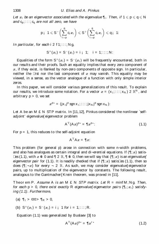
Let xi be an eigenvector associated with the eigenvalue ¶ i. Then, if 1 6 p 6 q 6 Nand cp; : : : ; cq are not all zero, we have

p ¡ 1 6 S¡µ qX

i= p

cixi

¶6 S +

µ qX

i = p

cixi

¶6 q ¡ 1:

In particular, for each i 2 f1; : : : ; Ng,

S + (xi) = S¡(xi) = i ¡ 1; i = 1; : : : ; N:

Equalities of the form S + (xi) = S¡(xi) will be frequently encountered, both inour results and their proofs. Such an equality implies that every zero component ofx, if they exist, is ®anked by non-zero components of opposite sign. In particular,neither the rst nor the last component of x may vanish. This equality may beviewed, in a sense, as the vector analogue of a function with only simple interiorzeros.

In this paper, we will consider various generalizations of this result. To explainour results, we introduce some notation. For a vector x = (x1; : : : ; xN ) 2 RN , andarbitrary p > 0, we set

xp¤ = (jx1jp sgn x1; : : : ; jxN jp sgn xN ):

Let A be an M £ N STP matrix. In [11,12], Pinkus considered the nonlinear `self-adjoint’ eigenvalue{eigenvector problem

AT(Ax)p ¤ = ¶ xp ¤ : (1.1)

For p = 1, this reduces to the self-adjoint equation

ATAx = ¶ x:

This problem (for general p) arose in connection with some n-width problems,and also has analogues as certain integral and di¬erential equations. If ( ¶ ; x) satis- es (1.1), with x 6= 0 and ¶ 2 R, ¶ 6= 0, then we will say that ( ¶ ; x) is an eigenvalue{eigenvector pair for (1.1). It is readily checked that if (¶ ; x) satis es (1.1), then sodoes (¶ ; ¬ x) for every ¬ 2 R. As such, we may consider eigenvalue{eigenvectorpairs, up to multiplication of the eigenvector by constants. The following result,analogous to the Gantmacher{Krein theorem, was proved in [11].

Theorem P. Assume A is an M £ N STP matrix. Let R = minfM; Ng. Then,for each p > 0, there exist exactly R eigenvalue{eigenvector pairs (¶ i; xi) satisfy-ing (1.1). Furthermore,

(a) ¶ 1 > ¢ ¢ ¢ > ¶ R > 0,

(b) S + (xi) = S¡(xi) = i ¡ 1 for i = 1; : : : ; R.

Equation (1.1) was generalized by Buslaev [3] to

AT(Ax)p ¤ = ¶ xr ¤ (1.2)

Nonlinear eigenvalue{eigenvector problems for STP matrices 1309

for arbitrary p; r > 0. Note that if ( ¶ ; x) satis es (1.2), then so does ( ¶ j¬ jp¡r; ¬ x).Because of this nonlinearity of the eigenvalue, when we talk about eigenvalue{eigenvector pairs, we will generally assume that kxk2 = 1 (the Euclidean normequals 1). Buslaev proved the following.

Theorem B. Assume A is an M £ N STP matrix. Let R = minfM; Ng. Then,for given p; r > 0 and each i 2 f1; : : : ; Rg, there exists at least one eigenvalue{eigenvector pair ( ¶ i; xi) satisfying (1.2), with ¶ i > 0 and S + (xi) = S¡(xi) = i ¡ 1.

For p 6= r, there may be many more than R eigenvalue{eigenvector pairs. Assuch, there may, and sometimes will, be more than one eigenvector with any xednumber of sign changes. Some examples are presented in x 5.

Two di¬erent proofs of the existence of eigenvalue{eigenvector pairs are givenin [11] and [12]. One depends on the Lyusternik{Schnirelman theorem on the cat-egory of an n-dimensional projective space. The other follows from an applicationof the implicit function theorem. The proof given by Buslaev is di¬erent and usesboth an ingenious xed-point argument and Borsuk’s antipodensatz theorem.

In this paper, we will consider certain generalizations of theorem P. In particular,we will consider the eigenvalue{eigenvector problem

Am(¢ ¢ ¢ (A2(A1x)p1 ¤ )p2 ¤ ¢ ¢ ¢ )pm ¡ 1 ¤ = ¶ xr ¤ ; (1.3)

where the p1; : : : ; pm¡1; r are arbitrary positive values and Ai is an Ni £ Ni¡1 STPmatrix, i = 1; : : : ; m, with N0 = Nm = N . Unfortunately, the lack of a certainform of `self-adjointness’, which is present in (1.1) and (1.2), renders the categoryargument in [11], and the xed-point and Borsuk arguments in [3], seemingly inap-plicable. We will use a variation on the argument from [12] that applies the implicitfunction theorem. As we will shall see, the existence, and not the uniqueness orcharacterization, is the major problem when considering (1.3).

Our main result is as follows.

Theorem 1.1. Assume that the Ai are as above, with p1; : : : ; pm¡1 > 1 andr = p1 ¢ ¢ ¢ pm¡1. Let R = minfNi : i = 1; : : : ; mg. Then there exist exactly Reigenvalue{eigenvector pairs ( ¶ i; xi) satisfying (1.3). Furthermore,

(a) ¶ 1 > ¢ ¢ ¢ > ¶ R > 0,

(b) S + (xi) = S¡(xi) = i ¡ 1 for i = 1; : : : ; R.

We conjecture that this same result holds for any positive p1; : : : ; pm¡1 andr = p1 ¢ ¢ ¢ pm¡1. While our proof uses the fact that the pi > 1, we will show howcertain additional cases follow from this result. For r 6= p1 ¢ ¢ ¢ pm¡1, there may bemany more eigenvalue{eigenvector pairs. We will also touch upon this brie®y.

Why do we consider only the particular nonlinear operation xp¤ ? If we demandthat if x is an eigenvector, then ¬ x is also an eigenvector for all ¬ 2 R (but withperhaps di¬erent eigenvalues), then we are led to a consideration of the functionalequation f (ab) = f(a)f(b) for all a; b 2 R. As is known (see, for example, [1, p. 41]),the only continuous solutions to this equation are

f(x) = jxjp


and

f(x) = jxjp sgn x = xp ¤ ;

for some 0 < p < 1. This is our reason for the choice of this operator.Before ending this introductory section, we recall two important properties of

STP matrices. These are called variation diminishing. This was Schoenberg’s initialcontribution to the theory. The versions we shall use are the following.

Theorem VD. Let A be an M £ N STP matrix. Then, for each vector x 2 RN ,x 6= 0,

S + (Ax) 6 S¡(x):

Furthermore if S + (Ax) = S¡(x), then the sign of the ¯rst (and last) componentof Ax (if zero, then the sign given in determining S + (Ax)) agrees with the sign ofthe ¯rst (and last) non-zero component of x.

We say that an M £ N matrix is STP of rank K if it is of rank K and all of itsr £ r minors are strictly positive for all r = 1; : : : ; K. An associated dual propertyto theorem VD is contained in this next result.

Theorem VD2. Let A be an M £ N STP matrix of rank K. If Ay = 0, theneither y = 0 or S¡(y) > K .

The two above results, and variants thereof, may be found in [2,9,13].This paper is organized as follows. In x 2 we provide a new proof of the Gant-

macher{Krein theorem. This is the `linear’ version of our problem. The standardmethod of proving the Gantmacher{Krein theorem is by the use of Perron’s theoremregarding the largest eigenvalue of a positive matrix, and its eigenvector, and Kro-necker’s theorem on the eigenvalues and eigenvectors of the associated compoundmatrices. In x 2 we will present an alternative method of proof for this theorem,which depends on neither of these results. It instead depends on the variation dimin-ishing property of STP matrices. In x 3, we consider generalizations of the methodof proof given in x 2, which permits us to prove the uniqueness and other propertiesof the solutions of the nonlinear problem (1.3) (always under the assumption thatr = p1 ¢ ¢ ¢ pm¡1). In x 4, we consider the problem of existence of solutions to (1.3).It is here that we apply the Gantmacher{Krein theorem (which is applicable in thecase p1 = ¢ ¢ ¢ = pm¡1 = r = 1) and the implicit function theorem, which permitsus to continue the solutions that exist in the former case to p1; : : : ; pm¡1 > 1 (andr = p1 ¢ ¢ ¢ pm¡1). This is used in the proof of theorem 1.1. We may totally foregothis restriction on the pi when dealing with the largest eigenvalue, or the smallesteigenvalue if all the Ai are invertible. We also rotate, and in certain cases, invert,the pi, and thus generalize theorem 1.1 to cover additional cases. In x 5 we brie®ydiscuss the case where r 6= p1 ¢ ¢ ¢ pm¡1, proving, for example, a Perron-type theoremif r > p1 ¢ ¢ ¢ pm¡1.

Somewhat analogous results for ordinary di¬erential equations may be foundin [4].


2. An alternative proof of the Gantmacher{Krein theorem

In this section, we provide a new and alternative proof of the Gantmacher{Kreintheorem. Let A be an N £N STP matrix. We start by proving that A has N simpleand positive eigenvalues. This part of the proof may be found in [10]. We use thenotation

A ¶

µi1; : : : ; ik

j1; : : : ; jk

¶

to denote the k £ k minor of the matrix A ¡ ¶ I , obtained by choosing the rowsi1; : : : ; ik and columns j1; : : : ; jk. From Sylvester’s determinant identity (see, forexample, [9, p. 3]), we have

A ¶

µ1; : : : ; N

1; : : : ; N

¶A¶

µ2; : : : ; N ¡ 1

2; : : : ; N ¡ 1

¶

= A ¶

µ1; : : : ; N ¡ 1

1; : : : ; N ¡ 1

¶A¶

µ2; : : : ; N

2; : : : ; N

¶¡ A¶

µ1; : : : ; N ¡ 1

2; : : : ; N

¶A¶

µ2; : : : ; N

1; : : : ; N ¡ 1

¶:

(2.1)

It is easily veri ed that

A¶

µ1; : : : ; N ¡ 1

2; : : : ; N

¶; A ¶

µ2; : : : ; N

1; : : : ; N ¡ 1

¶> 0 (2.2)

for all ¶ > 0. Expand each determinant as a polynomial in ¶ and note that all thecoe¯ cients of this polynomial are strictly positive, since all minors of A are strictlypositive.

We now use an induction argument to prove our result. We also simultaneouslyprove that the eigenvalues of the two principal minors obtained by deleting eitherthe rst row and column, or the last row and column, strictly interlace the eigen-values of the original matrix. The case N = 2 is easily checked.

For notational ease, set

p( ¶ ) = A ¶

µ1; : : : ; N

1; : : : ; N

¶;

q1( ¶ ) = A ¶

µ2; : : : ; N

2; : : : ; N;

¶;

q2( ¶ ) = A ¶

µ1; : : : ; N ¡ 1

1; : : : ; N ¡ 1

¶

and

r( ¶ ) = A ¶

µ2; : : : ; N ¡ 1

2; : : : ; N ¡ 1

¶:

We assume, by the induction hypothesis, that all the N ¡ 2 zeros of r are positiveand simple, and interlace the N ¡ 1 positive simple zeros of q1 and q2. Let

· 1 > ¢ ¢ ¢ > · N¡1 > 0


denote the zeros of either q1 or q2. From (2.1) and (2.2), it follows that

p(· i)r( · i) < 0; i = 1; : : : ; N ¡ 1:

Furthermore, as r(0) > 0 and by the induction hypothesis,

r( · i)( ¡ 1)i + N¡1 > 0; i = 1; : : : ; N ¡ 1;

implyingp( · i)( ¡ 1)i+ N > 0; i = 1; : : : ; N ¡ 1:

As p(0) > 0 and p( · N¡1) < 0, the polynomial p has an additional zero in (0; · N¡1).As p has leading coe¯ cient ( ¡ 1)N and p(· 1)( ¡ 1)N + 1 > 0, p also has a zero in( · 1; 1). Thus p has N positive simple zeros, which are interlaced by the N ¡ 1zeros of both q1 and q2. This proves the induction step, and thus A has N positivesimple eigenvalues.

We now assume that ¶ > · > 0 are eigenvalues, with associated linearly indepen-dent eigenvectors x and y. Then, from theorem VD, we have, for all ( ¬ ; ) 6= (0; 0),

S + (¶ ¬ x + · y) = S + (A(¬ x + y)) 6 S¡( ¬ x + y): (2.3)

Note that this implies

S + (x) = S¡(x) and S + (y) = S¡(y):

We now assume that both ¬ 6= 0 and 6= 0. We may rewrite (2.3) as

S +

µ¬ x +

µ·

¶

¶ y

¶6 S¡( ¬ x + y):

Iterating this process, we have

S +

µ¬ x +

µ·

¶

¶n

y

¶6 S¡(¬ x + y)

for every positive integer n. As n ! 1, and since · =¶ < 1 and S¡(x) = S + (x), itis easily veri ed that

limn ! 1

S +

µ¬ x +

µ·

¶

¶n

y

¶= S¡(x):

The above follows from the general fact (which we will use again) that if

limn ! 1

zn = z

and z 2 RN satis es S + (z) = S¡(z), then

S + (zn) = S¡(zn) = S + (z) = S¡(z) (2.4)

for n su¯ ciently large. Note that if " > 0 satis es

" < minfjzkj : zk 6= 0g;

then, for every n for which

maxfjznk ¡ zkj : k = 1; : : : ; Ng < ";


we necessarily have

S + (zn) = S¡(zn) = S + (z) = S¡(z):

Similarly, from (2.3),

S + (¬ x + y) 6 S¡µµ

·

¶

¶¬ x + y

¶

and, iterating this process, we obtain

S + (¬ x + y) 6 S¡µµ

·

¶

¶n

¬ x + y

¶

for every positive integer n. As n ! 1, and since · =¶ < 1 and S¡(y) = S + (y), itfollows that

limn ! 1

S¡µµ

·

¶

¶n

¬ x + y

¶= S¡(y):

Thus, for every ( ¬ ; ) 6= (0; 0),

S¡(x) 6 S¡( ¬ x + y) 6 S + (¬ x + y) 6 S¡(y):

If S¡(x) = S¡(y), then equality holds throughout our sequence of inequalities,and, in particular,

S + (¬ x + y) = S¡(¬ x + y)

for all ( ¬ ; ) 6= (0; 0). This is impossible, since there are choices of ¬ , for whichthe rst or last coe¯ cient of the vector ¬ x + y vanishes, in which case the aboveequality does not hold. Therefore, S¡(x) < S¡(y).

We have proved that A has N simple positive eigenvalues, and thus N associatedeigenvectors. For each of these N eigenvectors, we have

S + (x) = S¡(x) 2 f0; 1; : : : ; N ¡ 1g;

and if ¶ > · > 0 are eigenvalues with associated eigenvectors x and y, thenS¡(x) < S¡(y). This proves that if

¶ 1 > ¢ ¢ ¢ > ¶ N > 0

are the eigenvalues of A, and xi is an eigenvector associated with the eigenvalue¶ i, then

S + (xi) = S¡(xi) = i ¡ 1:

Now assume 1 6 p 6 q 6 N and we are given real constants cp; : : : ; cq, not allzero. Then, following the above analysis, repeated application of

S +

µ qX

i = p

ci ¶ ixi

¶= S +

µ qX

i= p

ciAxi

¶6 S¡

µ qX

i = p

cixi

¶

implies that

S¡µ qX

i= p

ci

µ¶ i

¶ p

¶n

xi

¶6 S¡

µ qX

i= p

cixi

¶6 S +

µ qX

i = p

cixi

¶6 S +

µ qX

i= p

ci

µ¶ q

¶ i

¶n

xi

¶:


We may assume that cp; cq 6= 0 and then apply

limn ! 1

S¡µ qX

i = p

ci

µ¶ i

¶ p

¶n

xi

¶= S¡(xp) = p ¡ 1;

while

limn ! 1

S +

µ qX

i = p

ci

µ¶ q

¶ i

¶n

xi

¶= S¡(xq) = q ¡ 1:

This implies

p ¡ 1 6 S¡µ qX

i= p

cixi

¶6 S +

µ qX

i = p

cixi

¶6 q ¡ 1;

which completes the proof of this theorem.

Remark 2.1. There is an additional result that is sometimes stated in connectionwith the Gantmacher{Krein theorem. It has to do with the `interlacing of the zeros’of xi+ 1 and xi, which is important in the continuous (integral) analogue of thistheorem. One form of this is the following. Let xi(t) be the continuous functionde ned on [1; N ], which is linear on each [j; j + 1], j = 1; : : : ; N ¡ 1, and such thatxi(j) is the jth component of xi. Since

S¡(xi) = S + (xi) = i ¡ 1;

the function xi(t) has exactly i ¡ 1 zeros, which are each strict sign changes. Since

i ¡ 1 6 S¡( ¬ xi + xi + 1) 6 S + ( ¬ xi + xi + 1) 6 i;

for every choice of (¬ ; ) 6= (0; 0) it can now be shown that the i ¡ 1 zeros of xi(t)strictly interlace the i zeros of xi + 1(t).

A similar argument proves the following variant, which we will need in x 4.

Theorem GK2. Let A be an N £N STP matrix of rank K. Then A has K positivesimple eigenvalues

¶ 1 > ¢ ¢ ¢ > ¶ K > 0

and, for the essentially unique eigenvector xi associated with the eigenvalue ¶ i,

S + (xi) = S¡(xi) = i ¡ 1; i = 1; : : : ; K:

3. Uniqueness and other properties

In this section, we will discuss uniqueness and certain associated properties for theproblem

Am(¢ ¢ ¢ (A2(A1x)p1 ¤ )p2 ¤ ¢ ¢ ¢ )pm ¡ 1 ¤ = ¶ xr ¤ ; (3.1)

where the pi are positive values and p1 ¢ ¢ ¢ pm¡1 = r. We show that the latter halfof the proof of theorem GK may be applied in this situation.

For ease of notation, we set

T (x) = Am(¢ ¢ ¢ (A2(A1x)p1 ¤ )p2 ¤ ¢ ¢ ¢ )pm ¡ 1 ¤ ;


where each Ai is an Ni £ Ni¡1 STP matrix, i = 1; : : : ; m, with N0 = Nm = N , andR = minfNi : i = 1; : : : ; mg. Note that

T ( ¬ x) = ¬ p1¢¢¢pm ¡ 1 ¤ T (x) = ¬ r ¤ T (x):

Thus ( ¶ ; x) is an eigenvalue{eigenvector pair for (3.1) if

T (x) = ¶ xr ¤ ;

and if ( ¶ ; x) is an eigenvalue{eigenvector pair, then, for every ¬ 2 R n f0g, so is( ¶ ; ¬ x).

Proposition 3.1. Under the above assumptions, let ( ¶ ; x) and (· ; y) be eigen-value{eigenvector pairs for (3.1). Assume x, y are linearly independent. Then, forall ( ¬ ; ) 6= (0; 0),

S + ( ¶ ¬ r ¤ xr ¤ + · ¬ r ¤ yr ¤ ) 6 S¡( ¬ x + y):

Proof. In this proof, we will use the easily checked

sgn(ap ¤ + bp ¤ ) = sgn(a + b) (3.2)

for any a; b 2 R and p > 0. We also recall that we are assuming that ¶ ; · 6= 0.We start by noting that since ( ¶ ; x) and ( · ; y) are eigenvalue{eigenvector pairs

for (3.1),¶ ¬ r ¤ xr ¤ + · ¬ r ¤ yr ¤ = T ( ¬ x) + T ( y):

Thus

S + ( ¶ ¬ r ¤ xr ¤ + · ¬ r ¤ yr ¤ ) = S + (T (¬ x) + T ( y))

= S + (Am(¢ ¢ ¢ (A2(A1( ¬ x))p1 ¤ )p2 ¤ ¢ ¢ ¢ )pm ¡ 1 ¤

+ Am(¢ ¢ ¢ (A2(A1( y))p1 ¤ )p2 ¤ ¢ ¢ ¢ )pm ¡ 1 ¤ ):

From theorem VD applied to the matrix Am, the above quantity is less than orequal to

S¡((Am¡1 ¢ ¢ ¢ (A2(A1( ¬ x))p1 ¤ )p2 ¤ ¢ ¢ ¢ )pm¡ 1 ¤

+ (Am¡1 ¢ ¢ ¢ (A2(A1( y))p1 ¤ )p2 ¤ ¢ ¢ ¢ )pm ¡ 1 ¤ )

and, by (3.2), is equal to

S¡(Am¡1(¢ ¢ ¢ (A2(A1( ¬ x))p1 ¤ )p2 ¤ ¢ ¢ ¢ )p¤m ¡ 2

+ Am¡1(¢ ¢ ¢ (A2(A1( y))p1 ¤ )p2 ¤ ¢ ¢ ¢ )p¤m ¡ 2 ):

As S¡(w) 6 S + (w) for every vector w, we can now continue this process, eachtime peeling away an Ak and a power, until we reach

S¡(¬ x + y):

Let us now consider some consequences of this simple inequality.


Corollary 3.2. Assume ( ¶ ; x) is an eigenvalue{eigenvector pair for (3.1). Then¶ > 0, and

S¡(x) = S + (x) 6 R ¡ 1;

where R = minfNi : i = 1; : : : ; mg.

Proof. Put ¬ = 1 and = 0 in the proof of proposition 3.1. Then, starting withS + ( ¶ xr ¤ )(= S + (x)), we get a whole series of increasing inequalities, ending withS¡(x). As S¡(x) 6 S + (x), it therefore follows that this series of inequalities areequalities. That is, S¡(x) = S + ( ¶ xr ¤ ) = S + (x). Furthermore, from the case ofequality as stated in the second part of theorem VD, we obtain ¶ > 0.

From these series of equalities we also have, for each i 2 f1; : : : ; mg,

S + (x) = S + (Ai(¢ ¢ ¢ (A2(A1x)p1 ¤ )p2 ¤ ¢ ¢ ¢ )p¤i ¡ 1 ); (3.3)

where p0 = 1. As Ai(¢ ¢ ¢ (A2(A1x)p1 ¤ )p2 ¤ ¢ ¢ ¢ )p¤i¡ 1 is a non-zero vector in RNi ,

we must have S¡(x) = S + (x) 6 Ni ¡ 1. This is true for each i, and thereforeS¡(x) = S + (x) 6 R ¡ 1.

We have so far only considered eigenvalue{eigenvector pairs with positive (non-zero) eigenvalues. What, if anything, can we say about those vectors satisfyingT (x) = 0?

Corollary 3.3. If T (x) = 0, then S¡(x) > R.

Proof. Starting with

T (x) = Am(¢ ¢ ¢ (A2(A1x)p1 ¤ )p2 ¤ ¢ ¢ ¢ )pm ¡ 1 ¤ = 0;

we have, from theorem VD2, that either

Am¡1(¢ ¢ ¢ (A2(A1x)p1 ¤ )p2 ¤ ¢ ¢ ¢ )p¤m ¡ 2 = 0

or this vector is not identically zero and

S¡(Am¡1(¢ ¢ ¢ (A2(A1x)p1 ¤ )p2 ¤ ¢ ¢ ¢ )p¤m¡ 2 ) > Nm:

In the latter case, we can repeatedly apply theorem VD and (3.2), as in the proofof proposition 3.1, to obtain

S¡(x) > S¡(Am¡1(¢ ¢ ¢ (A2(A1x)p1 ¤ )p2 ¤ ¢ ¢ ¢ )p¤m ¡ 2 ) > Nm > R;

since R = minfNi : i = 1; : : : ; mg. If

Am¡1(¢ ¢ ¢ (A2(A1x)p1 ¤ )p2 ¤ ¢ ¢ ¢ )p¤m ¡ 2 = 0;

then we continue as above (stripping away the Am¡1). It follows, in all cases, thatS¡(x) > R.

The main consequence of proposition 3.1 is the following result.

Theorem 3.4. In the eigenvalue{eigenvector problem (3.1), to each eigenvaluethere corresponds an essentially unique eigenvector. Furthermore, if ( ¶ ; x) and( · ; y) are eigenvalue{eigenvector pairs for (3.1) and ¶ > · , then S¡(x) < S¡(y) 6R ¡ 1.


Proof. From proposition 3.1, we have

S + ( ¶ ¬ r ¤ xr ¤ + · ¬ r ¤ yr ¤ ) 6 S¡( ¬ x + y);

which we can rewrite, by (3.2) (and since ¶ ; · > 0), as

S + (¶ 1=r ¬ x + · 1=r ¬ y) 6 S¡( ¬ x + y): (3.4)

Assume x, y are linearly independent eigenvectors associated with the sameeigenvalue ¶ > 0. Then, from (3.4),

S + (¬ x + y) 6 S¡(¬ x + y)

for all (¬ ; ) 6= (0; 0). But this is impossible, as this would imply, for example, thatthe rst and last coe¯ cients of the vector ¬ x + y never vanish. This contradic-tion implies that the eigenvector associated with the eigenvalue ¶ is unique (up tomultiplication by a constant).

Assume now that (¶ ; x) and ( · ; y) are eigenvalue{eigenvector pairs for (3.1), with¶ > · . We apply the same argument as may be found in our proof of theorem GK.For ¬ 6= 0, 6= 0, we have, by (3.4),

S +

µ¬ x +

µ·

¶

¶1=r

¬ y

¶6 S¡( ¬ x + y):

Iterating this process, we have

S +

µ¬ x +

µ·

¶

¶n=r

¬ y

¶6 S¡( ¬ x + y)

for every positive integer n. As n ! 1 and since · =¶ < 1 and S¡(x) = S + (x), itfollows by (2.4) that

limn ! 1

S +

µ¬ x +

µ·

¶

¶n=r

¬ y

¶= S¡(x):

Similarly,

S + ( ¬ x + y) 6 S¡µµ

·

¶

¶1=r

¬ x + y

¶

and, iterating this process, we obtain

S + ( ¬ x + y) 6 S¡µµ

·

¶

¶n=r

¬ x + y

¶

for every positive integer n. As n ! 1 and since · =¶ < 1 and S¡(y) = S + (y), itfollows that

limn ! 1

S¡µµ

·

¶

¶n=r

¬ x + y

¶= S¡(y):

Thus, for all ( ¬ ; ) 6= (0; 0),

S¡(x) 6 S¡( ¬ x + y) 6 S + (¬ x + y) 6 S¡(y):


If S¡(x) = S¡(y), then equality holds throughout and, in particular,

S + (¬ x + y) = S¡(¬ x + y)

for all (¬ ; ) 6= (0; 0), which is again impossible. Therefore, S¡(x) < S¡(y). Fromcorollary 3.2, we have S¡(y) 6 R ¡ 1.

4. Existence

In this section, we prove the existence of R distinct eigenvalue{eigenvector pairs forthe problem

T (x) = Am(¢ ¢ ¢ (A2(A1x)p1 ¤ )p2 ¤ ¢ ¢ ¢ )pm ¡ 1 ¤ = ¶ xr ¤ ; (4.1)

where the pi > 1 and p1 ¢ ¢ ¢ pm¡1 = r. This result, together with theorem 3.4,implies the existence of exactly R such pairs and proves theorem 1.1.

In the proof of the existence, we will use a method of proof based on the implicitfunction theorem. This proof is rather technical. We shall assume, in what follows,that each pi > 1. We may do this because, if pi = 1, then we simply reduce thenumber of terms in the above equation. For each t 2 [0; 1], we will set

pi(t) = pit + (1 ¡ t)

for i = 1; : : : ; m ¡ 1, and

r(t) = p1(t) ¢ ¢ ¢ pm¡1(t):

Note that

(p1(1); : : : ; pm¡1(1); r(1)) = (p1; : : : ; pm¡1; r);

while

(p1(0); : : : ; pm¡1(0); r(0)) = (1; : : : ; 1; 1):

By theorem GK2, we know the solutions of (4.1) for (p1(0); : : : ; pm¡1(0); r(0)). Wecontinue these solutions as functions of t until we reach (p1(1); : : : ; pm¡1(1); r(1)).

De ne, for k = 1; : : : ; N ,

Gk(x; ¶ ; t) = [Am(¢ ¢ ¢ (A2(A1x)p1(t) ¤ )p2(t)¤ ¢ ¢ ¢ )pm ¡ 1(t)¤ ¡ ¶ xr(t) ¤ ]k; (4.2)

and

GN + 1(x; ¶ ; t) =

NX

k = 1

jxkj2 ¡ 1: (4.3)

Solving (4.1) is equivalent to solving Gk(x; ¶ ; t) = 0 for k = 1; : : : ; N . The conditionGN + 1(x; ¶ ; t) = 0 is a normalization condition.

Now,

G(x; ¶ ; t) = (G1(x; ¶ ; t); : : : ; GN + 1(x; ¶ ; t)) 2 C(RN + 2; RN + 1):


As we will use the implicit function theorem for G(x; ¶ ; t) = 0 with respect to theN + 1 variables x1; : : : ; xN ; ¶ as functions of t, we must show that

G(x; ¶ ; t) = (G1(x; ¶ ; t); : : : ; GN + 1(x; ¶ ; t)) 2 C1(RN + 2; RN + 1):

We will do this explicitly by calculating most of the partial derivatives, since weneed them later.

We introduce the following notation. For k = 1; : : : ; m, we let Dk(x) be theNk £ Nk diagonal matrix whose diagonal entries are the components of the vector

Ak(Ak¡1 ¢ ¢ ¢ (A2(A1x)p1 ¤ )p2 ¤ ¢ ¢ ¢ )pk ¡ 1 ¤ ;

which is in RNk (and we set p0 = 1 so that D1(x) is the N1 £ N1 diagonal matrixwhose entries are the components of A1x). Thus the diagonal entries of Dm(x) arethe components of the vector T (x). When we write

jDk(x)jpk¡1;

it is to be understood that the operator j ¢ jpk¡1 is being applied to each element ofthis diagonal matrix. We will also drop the t from the pi(t), except when necessary.

The above notation is convenient since, for example, for p1 > 1,

@

@x`((A1x)p1 ¤ )k = p1j(A1x)kjp1¡1(A1)k;` = p1(jD1(x)jp1¡1A1)k;`:

Using this notation, and the calculations as above, we can write, for k; ` = 1; : : : ; N(and all pi > 1),

@Gk

@x`(x; ¶ ; t) = r(AmjDm¡1(x)jpm ¡ 1¡1Am¡1jDm¡2(x)jpm ¡ 2¡1

¢ ¢ ¢ A2jD1(x)jp1¡1A1)k;` ¡ ¶ rjx`jr¡1 ¯ `;k: (4.4)

For k = N + 1 and ` = 1; : : : ; N , we have

@GN + 1

@x`(x; ¶ ; t) = 2x`: (4.5)

As the variables are x1; : : : ; xN and ¶ , it will sometimes be convenient to use thenotation ¶ = xN + 1. For k = 1; : : : ; N and ` = N + 1, we see that

@Gk

@¶(x; ¶ ; t) =

@Gk

@xN + 1(x; ¶ ; t) = ¡ xr ¤

k ; (4.6)

while for k; ` = N + 1,@GN + 1

@xN + 1(x; ¶ ; t) = 0: (4.7)

It is also true that@Gk

@t(x; ¶ ; t)

is a continuous function. As we do not need its explicit value, we will not preciselycalculate it.


Note that, for all t 2 (0; 1], we have pi(t) > 1, and thus G(x; ¶ ; t) is a C1 functionin all its variables. At the pi(0) = 1, there is a problem in that G(x; ¶ ; 0) is notnecessarily C1. To be more precise, we have a problem with the continuity of theelements of jDk(x)jpk(t)¡1 and jxkjr(t)¡1 if some of their components tend to zeroas t ! 0. However, it is readily veri ed that G(x; ¶ ; 0) is locally C1 at thosevalues of x for which the components x and the diagonal components of Dk(x),all k = 1; : : : ; m, are not zero. We will consider the case where the pi(t) > 1,i.e. t 2 (0; 1], although, as we will note later, the analysis also applies to the casepi = 1 (and also to the cases pi < 1) at those x for which it and the diagonal entriesof the Dk(x) have no zero components.

Proposition 4.1. Let ~x 2 RN , ~¶ > 0 and ~t 2 (0; 1] be such that

G(~x; ~¶ ; ~t) = 0: (4.8)

Then

det

µ@Gk

@x`

¶N + 1

k;` = 1

¯̄¯̄(~x;~¶ ;~t)

6= 0: (4.9)

Proof. Set

bk` =1

r

@Gk

@x`

¯̄¯̄(~x;~¶ ;~t)

= (AmjDm¡1(~x)jpm ¡ 1¡1Am¡1jDm¡2(~x)jpm ¡ 2¡1

¢ ¢ ¢ A2jD1(~x)jp1¡1A1)k;`

and B = (bk`) for k; ` = 1; : : : ; N . Note that B is the product of STP matrices anddiagonal matrices with non-negative diagonal entries.

Assume (4.9) does not hold. Thus there exists a z = (z1; : : : ; zN + 1) 6= 0 in RN + 1

for which µ@Gk

@x`

¶N + 1

k;` = 1

¯̄¯̄(~x;~¶ ;~t)

z = 0:

We will contradict this fact.Assuming the above Jacobian is singular, then the above system of equations

may be rewritten, using (4.4){(4.7), as

NX

=̀ 1

bk`z` = ~¶ j~xkjr¡1zk ¡ ~xr ¤k

rzN + 1; (4.10)

which we will rewrite as

NX

` = 1

bk`z` = ~¶ j~xkjr¡1

µzk ¡ zN + 1 ~xk

~¶ r

¶; (4.11)

for k = 1; : : : ; N , andNX

` = 1

~x`z` = 0: (4.12)


We also have that (~x; ~¶ ; ~t) is a solution of (4.8). This we may rewrite as

NX

` = 1

bk`~x` = ~¶ j~xkjr¡1 ~xk; (4.13)

for k = 1; : : : ; N , andNX

=̀ 1

~x`~x` =

NX

=̀ 1

~x2` = 1: (4.14)

Equations (4.13) are obtained via

NX

` = 1

bk`~x` =

NX

` = 1

(AmjDm¡1(~x)jpm ¡ 1¡1Am¡1jDm¡2( ~x)jpm ¡ 2¡1

¢ ¢ ¢ A2jD1(~x)jp1¡1A1)k;`~x`

= (AmjDm¡1( ~x)jpm¡ 1¡1Am¡1jDm¡2(~x)jpm ¡ 2¡1 ¢ ¢ ¢ A2jD1(~x)jp1¡1A1 ~x)k:

Now we apply

jD1( ~x)jp1¡1A1 ~x = (A1 ~x)p¤1 ;

and

jD2( ~x)jp2¡1A2(A1 ~x)p¤1 = (A2(A1 ~x)p¤

1 )p¤2 ;

etc.Set

~z = (z1; : : : ; zN )

(leaving o¬ zN + 1) and recall that

~x = (~x1; : : : ; ~xN ):

If ~z = (z1; : : : ; zN ) = 0, then (4.10) reduces to

0 = ¡ ~xr ¤k

rzN + 1

for k = 1; : : : ; N , which, in turn, implies that zN + 1 = 0. This would contradict thesingularity of the Jacobian and prove (4.9). We will prove that ~z = 0.

Suppose ~z 6= 0. From (4.12) and (4.14), it follows that ~x and ~z are linearlyindependent. We divide the remaining proof of this proposition into the two cases:zN + 1 = 0 and zN + 1 6= 0.

Case 1 (zN + 1 = 0). In this case, equation (4.11) reduces to

NX

` = 1

bk`z` = ~¶ j~xkjr¡1zk (4.15)

for k = 1; : : : ; N . We recall that we also have

NX

=̀ 1

bk` ~x` = ~¶ j~xkjr¡1 ~xk (4.13)


for k = 1; : : : ; N . Next we shall follow an analysis similar to that in the proof ofproposition 3.1 to obtain, for all ( ¬ ; ) 6= (0; 0),

S¡(¬ ~x + ~z) = S + ( ¬ ~x + ~z): (4.16)

As we noted in the previous section, equation (4.16) cannot hold for all ( ¬ ; ) 6=(0; 0), and thus we are led to a contradiction.

To obtain (4.16), we argue as follows. Firstly,

S + ( ¬ ~x + ~z) 6 S + (f~¶ j~xkjr¡1( ¬ ~xk + zk)gNk = 1);

since we have multiplied each component of the vector on the left by a positivevalue, or made it zero. From (4.13) and (4.15), the above is equal to

S + (B( ¬ ~x + ~z)) = S + (AmjDm¡1( ~x)jpm ¡ 1¡1Am¡1jDm¡2(~x)jpm ¡ 2¡1

¢ ¢ ¢ A2jD1(~x)jp1¡1A1( ¬ ~x + ~z)):

From theorem VD (applied to the matrix Am), we obtain an upper bound that isless than or equal to

S¡(jDm¡1(~x)jpm ¡ 1¡1Am¡1jDm¡2( ~x)jpm ¡ 2¡1 ¢ ¢ ¢ A2jD1( ~x)jp1¡1A1(¬ ~x + ~z)):

As jDm¡1( ~x)jpm¡ 1¡1 is a diagonal matrix with non-negative entries, it follows thatthe above is less than or equal to

S¡(Am¡1jDm¡2(~x)jpm ¡ 2¡1 ¢ ¢ ¢ A2jD1(~x)jp1¡1A1( ¬ ~x + ~z));

which is less than or equal to

S + (Am¡1jDm¡2( ~x)jpm ¡ 2¡1 ¢ ¢ ¢ A2jD1( ~x)jp1¡1A1(¬ ~x + ~z)):

We continue, peeling away the Ak followed by the jDk¡1(~x)jpk ¡ 1¡1, until we nallyreach

S¡( ¬ ~x + ~z):

The above argument is valid if none of the vectors along the way are identicallyzero. This is because theorem VD only holds for non-zero vectors. Let us thereforesuppose that, somewhere along the way, one of these vectors is identically zero.Then, necessarily,

~¶ j~xkjr¡1( ¬ ~xk + zk) = 0

for k = 1; : : : ; N , which we rewrite (since ~¶ 6= 0 and r > 1) as

~xk(¬ ~xk + zk) = 0 (4.17)

for k = 1; : : : ; N . Thus, if ~xk 6= 0, then

zk = ¡ ¬

~xk

(and 6= 0). From (4.12) (and (4.14)),

0 =

NX

` = 1

~x`z` =

NX

` = 1

~x`

µ¡ ¬

~x`

¶= ¡ ¬

NX

` = 1

~x2` = ¡ ¬

;


and thus ¬ = 0. Therefore, equation (4.17) reduces to

~xkzk = 0 (4.18)

for all k = 1; : : : ; N .Each Ak is STP and each jDk(~x)jpk¡1 is a diagonal matrix with positive or zero

entries. As such, it follows that B is an N £ N matrix of rank K, which is STP oforder K, i.e. all its r £ r minors are strictly positive for all r 2 f1; : : : ; Kg. K is, infact, the minimum of the Ni and the number of non-zero diagonal entries in eachof the Dk(~x). As B ~z = 0, this implies, from theorem VD2, that S¡(~z) > K.

We set ¬ = 1 and = 0 in the above series of inequalities (in which case, wealways have equality and the vectors never identically vanish), and obtain

S¡( ~x) = S + (~x)

= S¡(Ak(¢ ¢ ¢ (A2(A1(x))p1 ¤ )p2 ¤ ¢ ¢ ¢ )p¤k¡ 1 )

= S + (Ak(¢ ¢ ¢ (A2(A1(x))p1 ¤ )p2 ¤ ¢ ¢ ¢ )p¤k ¡ 1 ) (4.19)

for k = 1; : : : ; m. Equivalently, equation (4.19) may be obtained from (3.3) in theproof of corollary 3.2, applied to the eigenvalue{eigenvector pair (~¶ ; ~x). As theDk(~x) are Nk £ Nk diagonal matrices whose diagonal entries are the componentsof the vector in (4.19), it follows that

S¡(~x) = S + ( ~x) 6 K ¡ 1:

Thus, from (4.18) and the above,

K + 1 6 S¡(~z) + 1 6 #fi : zi 6= 0g 6 #fi : ~xi = 0g 6 S + (~x) 6 K ¡ 1:

This is a contradiction. Thus (4.18) cannot hold. This completes the proof of (4.16),which, in turn, is a contradiction. Thus we have proved the result in the casezN + 1 = 0.

Case 2 (zN + 1 6= 0). We recall that, in this case, we have (4.11) and (4.13), i.e.

NX

=̀ 1

bk`z` = ~¶ j~xkjr¡1

µzk ¡ zN + 1 ~xk

~¶ r

¶(4.11)

and

NX

` = 1

bk`~x` = ~¶ j~xkjr¡1 ~xk (4.13)

for k = 1; : : : ; N . We also still have (4.12) and (4.14), which, of course, imply thatthe ~x and ~z are linearly independent.

We follow, in general, the analysis of the previous case to obtain, for all ( ¬ ; ) 6=(0; 0),

S +

µµ¬ ¡ zN + 1

~¶ r

¶~x + ~z

¶6 S¡(¬ ~x + ~z): (4.20)


Let us assume for the moment that (4.20) is valid. Why does this lead to a contra-diction?

Assuming (4.20) holds for all ( ¬ ; ) 6= (0; 0), we have the inequalities

S¡µµ

¬ ¡ (k + 1)zN + 1

~¶ r

¶~x + ~z

¶6 S +

µµ¬ ¡

(k + 1)zN + 1

~¶ r

¶~x + ~z

¶

6 S¡µµ

¬ ¡ kzN + 1

~¶ r

¶~x + ~z

¶

6 S +

µµ¬ ¡ kzN + 1

~¶ r

¶~x + ~z

¶;

which are valid for all k 2 Z. As S + (y); S¡(y) 2 f0; 1; : : : ; N ¡ 1g for every non-zerovector y 2 RN , it follows that

S¡µµ

¬ ¡ kzN + 1

~¶ r

¶~x + ~z

¶= S +

µµ¬ ¡ kzN + 1

~¶ r

¶~x + ~z

¶= m1 (4.21)

for all k > K1, and

S¡µµ

¬ ¡ kzN + 1

~¶ r

¶~x + ~z

¶= S +

µµ¬ ¡ kzN + 1

~¶ r

¶~x + ~z

¶= m2 (4.22)

for all k < K2. Assume 6= 0 (if = 0, there is nothing to prove), divide thevectors in (4.21) and (4.22) by k, and let k ! 1 and k ! ¡ 1, respectively. Then,recalling that (~¶ ; ~x) is an eigenvalue{eigenvector pair, and, from corollary 3.2,

S¡(~x) = S + (~x);

we obtain

S¡(~x) = S + (~x) = m1 = m2:

(See (2.4) in the proof of theorem GK.)Thus m1 = m2 and, as a consequence, we have equality throughout the above

series of inequalities for all k 2 Z. In particular, we obtain

S¡( ¬ ~x + ~z) = S + ( ¬ ~x + ~z) = m1

for all ( ¬ ; ) 6= (0; 0). But this is impossible for linearly independent ~x and ~z, anda contradiction ensues. Thus it remains to prove that (4.20) holds for all ( ¬ ; ) 6=(0; 0).

To obtain (4.20), we argue as follows. From (4.11) and (4.13),

S +

µµ¬ ¡ zN + 1

~¶ r

¶~x + ~z

¶6 S +

µ½~¶ j~xkjr¡1

µ¬ ~xk +

µzk ¡ zN + 1

~¶ r~xk

¶¶¾N

k = 1

¶

= S + (B( ¬ ~x + ~z)):

We now apply the series of inequalities as in case 1 until we nally reach

S¡( ¬ ~x + ~z):


As in case 1, the above is valid if none of the vectors along the way are identicallyzero. Again, this is because theorem VD only holds for non-zero vectors. The initialvectors

~x and ~z ¡ zN + 1

~¶ r~x

are linearly independent, since ~x and ~z are linearly independent. Thus, if any ofthe intermediate vectors are zero, then, necessarily,

~¶ j~xkjr¡1

·¬ ~xk +

µzk ¡ zN + 1

~¶ r~xk

¶¸= 0

for k = 1; : : : ; N , which we rewrite (since ~¶ 6= 0) as

~xk

·µ¬ ¡ zN + 1

~¶ r

¶~xk + zk

¸= 0 (4.23)

for k = 1; : : : ; N .From (4.23) and (4.14), it follows that if = 0, then ¬ = 0. Assuming 6= 0, we

have

z` = ¡ 1

µ¬ ¡ zN + 1

~¶ r

¶~x`

if ~x` 6= 0. But then, from (4.12) and (4.14),

0 =

NX

` = 1

~x`z` = ¡ 1

µ¬ ¡ zN + 1

~¶ r

¶ NX

` = 1

~x2` = ¡ 1

µ¬ ¡ zN + 1

~¶ r

¶:

Thus we must have

¬ ¡ zN + 1

~¶ r= 0:

Substituting in (4.23) we see that this implies

~xkzk = 0 (4.24)

for all k = 1; : : : ; N .Applying (4.24) to (4.11) we have

NX

` = 1

bk`z` = ¡ ~¶ j~xkjr¡1 zN + 1 ~xk

~¶ r; (4.25)

for k = 1; : : : ; N . From (4.25) it follows that

S¡(~x) = S + ( ~x) = S + (B ~z) 6 S¡(~z):

On the other hand, from (4.24),

S¡(~z) + 1 6 #fi : zi 6= 0g 6 #fi : ~xi = 0g 6 S + (~x);

and thusS¡(~z) < S + (~x):

We have arrived at a contradiction. This proves (4.20) for all ( ¬ ; ) 6= (0; 0) andcompletes the proof of the proposition.


As we noted before the statement of proposition 4.1, G(x; ¶ ; t) is not necessarilya C1 function at t = 0. This is a consequence of the fact that jyjp¡1 (which appearsin various guises in (4.4)) does not necessarily have a limit as both y ! 0 andp ! 1. Of course, if y ! y ¤ 6= 0, then this limit does exist (and equals 1). Theproof of proposition 4.1 in the case where ~x and Ak ¢ ¢ ¢ A1 ~x; k = 1; : : : ; m, have nozero components is much simpler since ~xkzk = 0 for k = 1; : : : ; N implies ~z = 0. Wewill not repeat this proof here. In fact, under the assumption of the non-vanishingof the components of the above vectors we can also apply the above analysis forany pi > 0, for all i, with r = p1 ¢ ¢ ¢ pm¡1. We state this in the special case of(p1(0); : : : ; pm¡1(0)) = (1; : : : ; 1) as we will rst use it to prove theorem 1.1.

Proposition 4.2. Let ~x 2 RN and ~¶ > 0 be such that

G(~x; ~¶ ; 0) = 0: (4.26)

Further assume that each of the vectors ~x and Ak ¢ ¢ ¢ A1 ~x; k = 1; : : : ; m, has nozero component. Then

det

µ@Gk

@x`

¶N + 1

k;` = 1

¯̄¯̄(~x;~¶ ;0)

6= 0: (4.27)

We can now prove theorem 1.1.

Proof of theorem 1.1. Let n 2 f0; : : : ; R ¡ 1g. From theorem GK2 the linear problemhas a solution. That is, there exists an x 2 RN and ¶ > 0 for which G(x; ¶ ; 0) = 0and S¡(x) = S + (x) = n.

Assume x and Ak ¢ ¢ ¢ A1x, k = 1; : : : ; m, have no zero components. Then fromproposition 4.2 and the implicit function theorem there exists a t¤ > 0 such thatfor all t 2 [0; t¤ ) there are continuously di¬erentiable functions of t, namely x(t)and ¶ (t) for which

G(x(t); ¶ (t); t) = 0:

Furthermore, since S¡(x) = S + (x) = n and ¶ > 0, we have S¡(x(t)) = S + (x(t)) =n for t near 0.

Let ~t > 0 be the largest value for which for all t 2 [0; ~t) there exist x(t) and ¶ (t)such that G(x(t); ¶ (t); t) = 0 and S¡(x(t)) = S + (x(t)) = n. We wish to prove ourresult for t = 1, and we thus want to show that ~t > 1. (In fact ~t = 1.) Assume~t 6 1. There then exists a subsequence tk " ~t such that along this subsequencex(tk) ! ~x and ¶ (tk) ! ~¶ . (The boundedness of x(t) is given by (4.3), and thatof ¶ (t) easily proved.) From the limiting process it easily follows that S¡(~x) 6n 6 S + (~x) and G(~x; ~¶ ; ~t) = 0: As (~¶ ; ~x) is an eigenvalue{eigenfunction pair wehave from corollaries 3.2 and 3.3 that S¡(~x) = S + (~x) = n and ~¶ > 0. We can nowagain apply the implicit function theorem using proposition 4.1, contradicting themaximality of ~t.

It remains for us to consider the case where some of the components of x andAk ¢ ¢ ¢ A1x, k = 1; : : : ; m, are equal to zero. This is a technical problem which weovercome by perturbation.

We rst appeal to lemma 6.6 in [12]. From the method of proof therein thereexists, for " > 0, small, Nk £ Nk¡1 STP matrices A"

k which tend to Ak as " # 0,


and x" 2 RN which tends to x as " # 0, such that

A"m ¢ ¢ ¢ A"

1x" = ¶ x";

where S¡(x") = n, and x" and A"k ¢ ¢ ¢ A"

1x", k = 1; : : : ; m, have no zero components.We can now apply the previous analysis to obtain a vector ~x" which satis es theresult of theorem 1.1 (S¡(~x") = S + (~x") = n) for p1; : : : ; pm¡1, but with the matri-ces Ak replaced by A"

k. We now let " # 0, and obtain (at least on a subsequence) alimiting vector ~x and value ~¶ which necessarily satis es

G(~x; ~¶ ; 1) = 0;

and S¡(~x) = S + (~x) = n. This proves theorem 1.1.

If some (or all) of the pi < 1, then the above method of proof is valid at those x forwhich none of the components of x nor the diagonal entries of Dk(x), k = 1; : : : ; m,vanish (see (4.4)). If S¡(x) = S + (x) = 0, and (¶ ; x) is an eigenvalue{eigenvectorpair, then x has no zero components, nor do the diagonal entries of Dk(x) forany k = 1; : : : ; m. Thus we immediately have the following result (which we willgeneralize in x 5).

Proposition 4.3. Assume the Ai are as in theorem 1.1 and r = p1 ¢ ¢ ¢ pm¡1. Thereexists exactly one eigenvalue{eigenvector pair ( ¶ ; x) satisfying (4.1) with x havingall positive components. Furthermore, if · is any other eigenvalue of (4.1), then¶ > · > 0.

If x = (x1; : : : ; xN ) 2 RN and S + (x) = S¡(x) = N ¡ 1, then xixi+ 1 < 0 andin particular none of its components vanish. This will also be true for the diagonalentries of Dk(x) for every k = 1; : : : ; m, if each is in RN and

S + (Ak(Ak¡1 ¢ ¢ ¢ (A2(A1x)p1 ¤ )p2 ¤ ¢ ¢ ¢ )pk ¡ 1 ¤ )

= S¡(Ak(Ak¡1 ¢ ¢ ¢ (A2(A1x)p1 ¤ )p2 ¤ ¢ ¢ ¢ )pk ¡ 1 ¤ )

= N ¡ 1:

These latter equalities will hold when ( ¶ ; x) is an eigenvalue{eigenvector pair,S + (x) = S¡(x) = N ¡ 1, and each of the Ai is an N £ N STP matrix. (See,for example, (3.3) and the method of proof of corollary 3.2.) As such we have thefollowing.

Proposition 4.4. Assume the Ai are N £ N STP matrices as in theorem 1.1 andr = p1 ¢ ¢ ¢ pm¡1. Then there exists exactly one eigenvalue{eigenvector pair ( ¶ ; x)satisfying (4.1) with S + (x) = S¡(x) = N ¡ 1. Furthermore, if · is any othereigenvalue of (4.1), then 0 < ¶ < · .

Let us rewrite (4.1) as

(Am(¢ ¢ ¢ (A2(A1x)p1 ¤ )p2 ¤ ¢ ¢ ¢ )pm¡ 1 ¤ )pm ¤ = ¶ x; (4.28)

where we have simply set pm = 1=r. (This ¶ is the previous ¶ to the power 1=r.)The condition p1 ¢ ¢ ¢ pm¡1 = r is rewritten as

p1 ¢ ¢ ¢ pm¡1pm = 1: (4.29)


We have proved theorem 1.1 under the assumption that pi > 1 for i = 1; : : : ; m ¡ 1(and thus pm 6 1). We conjecture that theorem 1.1 holds for all choices of pi > 0satisfying (4.29). We can generalize theorem 1.1 to the following cases.

Proposition 4.5. Assume p1 ¢ ¢ ¢ pm = 1, and exactly one of the pi is strictly lessthan 1. Then the results of theorem 1.1 hold.

Proof. We show that starting with (4.28) we can `rotate’ the fpigmi = 1. We do this

by settingy = (A1x)p1 ¤ :

Multiplying (4.28) by A1 and raising both sides thereof to the power p1¤, we get

(A1(Am(¢ ¢ ¢ (A2y)p2 ¤ ¢ ¢ ¢ )pm ¡ 1 ¤ )pm ¤ )p1 ¤ = ¶ p1 y: (4.30)

If we assume that pk < 1, while all the other pi > 1, then we can rotate as aboveuntil the powers are in the order pk + 1; : : : ; pm; p1; : : : ; pk. We now raise both sidesof the equation to the power 1=pk¤ and apply theorem 1.1.

Furthermore, it is easily checked that if ( ¶ ; x) is an eigenvalue{eigenvector pairfor (4.28) with S + (x) = S¡(x) = r, then ( ¶ p1 ; y) is an eigenvalue{eigenvector pairfor (4.30) with S + (y) = S¡(y) = r. Since we may continue to rotate, eventuallyarriving back at (4.28), it is also true that if ( ¶ p1 ; y) is an eigenvalue{eigenvectorpair for (4.30) with S + (y) = S¡(y) = r, then ( ¶ ; x) is an eigenvalue{eigenvectorpair for (4.28). We apply this type of argument to translate our N eigenvalue{eigenvector pairs obtained from our application of theorem 1.1 back to (4.28).

If we assume that each Ai is an N £ N STP matrix (and thus invertible), thenwe also have the following.

Proposition 4.6. Assume p1 ¢ ¢ ¢ pm = 1, and exactly one of the pi is strictlygreater than 1. If each Ai is an N £ N STP matrix, then the results of theorem 1.1hold.

Proof. As the Ai are invertible, we shall invert (4.28) and then apply proposi-tion 4.5.

Inverting each of the Ai, and then raising it to the appropriate power, it is readilyveri ed that (4.28) is equivalent to

B1(¢ ¢ ¢ (Bm(x)qm ¤ )qm ¡ 1 ¤ ¢ ¢ ¢ )q1 ¤ =1

¶x; (4.31)

where Bi = A¡1i and qi = 1=pi, i = 1; : : : ; m. If A is any N £ N STP matrix and

B = A¡1, then JBJ is an N £ N STP matrix, where J is the diagonal matrix withith diagonal entry equal to ( ¡ 1)i. Set Ci = JBiJ , i = 1; : : : ; m, and y = Jx. Then(4.31) (and thus (4.28)) is equivalent to

C1(¢ ¢ ¢ (Cm(y)qm ¤ )qm ¡ 1 ¤ ¢ ¢ ¢ )q1 ¤ =1

¶y: (4.32)

Furthermore, S + (x) = S¡(x) = i ¡ 1 if and only if S + (y) = S¡(y) = N ¡ i. Asexactly one of the pi is in value greater than 1, then exactly one of the qi is in valueless than 1, and we can apply proposition 4.5 to obtain the desired result.


5. The non-homogeneous case

In this section we consider the equation

T (x) = Am(¢ ¢ ¢ (A2(A1x)p1 ¤ )p2 ¤ ¢ ¢ ¢ )pm ¡ 1 ¤ = ¶ xr ¤ ; (5.1)

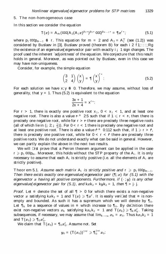
where p1 ¢ ¢ ¢ pm¡1 6= r. This equation for m = 2 and A2 = AT1 (see (1.2)) was

considered by Buslaev in [3]. Buslaev proved (theorem B) for each i 2 f1; : : : ; Rgthe existence of an eigenvalue{eigenvector pair with exactly i ¡ 1 sign changes. Theproof used the inherent `adjointness’ of the equation. We conjecture that this resultholds in general. Moreover, as was pointed out by Buslaev, even in this case wemay have non-uniqueness.

Consider, for example, the simple equationµ

3 1

2 4

¶ µx

y

¶= ¶

µx

y

¶r ¤

: (5.2)

For each solution we have x; y 6= 0. Therefore, we may assume, without loss ofgenerality, that y = 1. Thus (5.2) is equivalent to the equation

3x + 1

2x + 4= xr ¤ :

For r > 1, there is exactly one positive root x1, 0 < x1 < 1, and at least onenegative root. There is also a value ~r º 2:5 such that if 1 6 r < ~r, then there isprecisely one negative root, while for r > ~r there are precisely three negative roots(all of which lie in (¡ 2; ¡ 1

3)). For 0 < r < 1 there is precisely one negative root and

at least one positive root. There is also a value r̂ º 0:112 such that, if 1 > r > r̂,there is precisely one positive root, while for 0 < r < r̂ there are precisely threepositive roots. We do not understand exactly what can be said in general. However,we can partly explain the above in the next two results.

We will rst prove that a Perron theorem argument can be applied in the caser > p1 ¢ ¢ ¢ pm. Moreover, this holds without the STP property of the Ai. It is onlynecessary to assume that each Ai is strictly positive (i.e. all the elements of Ai arestrictly positive).

Theorem 5.1. Assume each matrix Ai is strictly positive and r > p1 ¢ ¢ ¢ pm¡1.Then there exists exactly one eigenvalue{eigenvector pair ( ¶ ; x) for (5.1) with theeigenvector x having all positive components. Furthermore, if (· ; y) is any othereigenvalue{eigenvector pair for (5.1), and kxk2 = kyk2 = 1, then ¶ > j· j.

Proof. Let ¤ denote the set of all ¶ > 0 for which there exists a non-negativevector x satisfying kxk2 = 1 and T (x) > ¶ xr. It is easily veri ed that ¤ is non-empty and bounded. As such it has a supremum which we will denote by ¶ 0.Let ¶ k be a sequence of values in ¤ which increase to ¶ 0. By de nition thereexist non-negative vectors xk satisfying kxkk2 = 1 and T (xk) > ¶ kxr

k. Takingsubsequences, if necessary, we may assume that limk ! 1 xk = x0. Thus kx0k2 = 1and T (x0) > ¶ 0xr

0.We claim that T (x0) = ¶ 0xr

0. Assume not. Set

y0 = (T (x0))1=r > ¶1=r0 x0:


As y0 is not equal to ¶1=r0 x0 it follows that

T (y0) > T (¶1=r0 x0) = ¶

p1¢¢¢pm ¡ 1=r0 T (x0) = ¶

p1¢¢¢pm ¡ 1=r0 yr

0:

However, ky0k2 6= 1 and so this inequality does not yet tell us much.Set

z0 = ¬ y0;

where kz0k2 = 1, i.e. ¬ = ky0k¡12 . Thus

T (z0) = ¬ p1¢¢¢pm ¡ 1 T (y0) > ¬ p1¢¢¢pm ¡ 1 ¶p1¢¢¢pm ¡ 1=r0 yr

0 = ¬ p1¢¢¢pm ¡ 1¡r ¶p1¢¢¢pm ¡ 1=r0 zr

0 :

Now y0 > ¶1=r0 x0 > 0 and therefore

1

¬= ky0k2 > ¶

1=r0 kx0k2 = ¶

1=r0 ;

i.e. ¬ ¶1=r0 < 1. By assumption p1 ¢ ¢ ¢ pm¡1 ¡ r < 0. Thus

¬ p1¢¢¢pm ¡ 1¡r ¶p1¢¢¢pm ¡ 1=r0 > ¶ 0:

We have contradicted our de nition of ¶ 0. Thus ( ¶ 0; x0) is an eigenvalue{eigenvectorpair for (5.1) with x0 strictly positive and kx0k2 = 1. This completes the existenceproof.

If T (y) = · yr ¤ and kyk2 = 1, then setting

jyj = (jy1j; : : : ; jyN j);

it easily follows thatT (jyj) > j· jjyjr;

and of course kjyjk2 = 1. Thus by de nition ¶ 0 > j· j. If ¶ 0 = j· j, then we musthave T (jyj) = ¶ 0jyjr and y must be a vector of one sign.

It therefore remains to prove that there can only be one eigenvalue{eigenvectorpair having all positive components.

Assume ( ¶ ; x) and ( · ; y) are eigenvalue{eigenvector pairs having all positive com-ponents, with kxk2 = kyk2 = 1, x, y linearly independent, and ¶ 6 · . Choose ¬ > 0such that ¬ x ¡ y remains a positive vector, but ® x ¡ y is not positive for every® < ¬ . Note that as kxk2 = kyk2 = 1 and x, y are linearly independent, it followsthat ¬ > 1. Since the Ai are strictly positive matrices we have

¬ p1¢¢¢pm ¡ 1 ¶ xr = T (¬ x) > T (y) = · yr:

Thus, the vector ¶ ¬ p1¢¢¢pm ¡ 1 xr ¡ · yr is strictly positive, implying

µ¶

·

¶1=r

¬ p1¢¢¢pm ¡ 1=r > ¬ :

As r > p1 ¢ ¢ ¢ pm¡1 and ¬ > 1, this implies that

¶ > · :

But this contradicts our assumption. Thus there is at most one eigenvalue{eigen-vector pair (¶ ; x) with the vector x having all positive components.


If the Ai are N £N STP matrices, then we can invert (5.1), as in proposition 4.6,and then apply theorem 5.1 to the smallest eigenvalue. We then obtain the followingcorollary.

Corollary 5.2. Assume each Ai is an N £ N STP matrix and p1 ¢ ¢ ¢ pm¡1 >r. Then there exists exactly one eigenvalue{eigenvector pair ( ¶ ; x) for (5.1) withS + (x) = S¡(x) = N ¡ 1. Furthermore, if ( · ; y) is any other eigenvalue{eigenvectorpair for (5.1), and kxk2 = kyk2 = 1, then ¶ < j· j.

Acknowledgments

This research was supported by the Fund for the Promotion of Research at theTechnion.

References

1 J. Acz¶el. Lectures on functional equations and their applications (Academic, 1966).

2 T. Ando. Totally positive matrices. Linear Algebra Applic. 90 (1987), 165{219.

3 A. P. Buslaev. A variational description of the spectra of totally positive matrices, andextremal problems of approximation theory. Mat. Zametki 47 (1990), 39{46. (Transl. Math.Notes 47 (1990), 26{31.)

4 U. Elias and A. Pinkus. Nonlinear eigenvalue problems for a class of ordinary di® erentialequations. Proc. R. Soc. Edinb. A 132 (2002), 1333{1359. (This issue.)

5 F. R. Gantmacher and M. G. Krein. Sur les matrices oscillatoires. C. R. Hebd. Seanc. Acad.Sci. Paris 201 (1935), 577{579.

6 F. R. Gantmacher and M. G. Krein. Sur les matrices complµetement non n¶egatives et oscil-latoires. Compositio Math. 4 (1937), 445{476.

7 F. R. Gantmacher and M. G. Krein. Oscillation matrices and small oscillations of mechan-ical systems (Moscow: Gostekhizdat, 1941). (In Russian.)

8 F. R. Gantmacher and M. G. Krein. Ostsillyatsionye Matritsy i Yadra i Malye KolebaniyaMekhanicheskikh Sistem (Moscow: Gosudarstvenoe Izdatel’ stvo 1950). (Transl. Oscillationmatrices and kernels and small vibrations of mechanical systems (USAEC, 1961).)

9 S. Karlin. Total positivity, vol. 1 (Stanford University Press, 1968).

10 D. M. Koteljanskii. Some su± cient conditions for reality and simplicity of the spectrum ofa matrix. Am. Math. Soc. Transl. 2 27 (1963), 35{42.

11 A. Pinkus. Some extremal problems for strictly totally positive matrices. Linear AlgebraApplic. 64 (1985), 141{156.

12 A. Pinkus. n-widths of Sobolev spaces in Lp . Constr. Approx. 1 (1985), 15{62.

13 I. J. Schoenberg. �Uber variationsvermindernde lineare Transformationen. Math. Z. 32(1930), 321{328.

14 I. J. Schoenberg. I. J. Schoenberg: selected papers (ed. C. de Boor) (Birkh�auser, 1988).

(Issued 13 December 2002)

Date post:	14-Apr-2018
Category:	Documents
Upload:	vuongdiep
View:	226 times
Download:	2 times

Nonlinear eigenvalue-eigenvector problems for STP …pinkus/papers/ev-STP.pdf ·...

Documents