Page 1
Nonlinear ion-acoustic solitons in a magnetized quantum plasma
with arbitrary degeneracy of electrons
Fernando Haas
Physics Institute, Federal University of Rio Grande do Sul,
CEP 91501-970, Av. Bento Goncalves 9500, Porto Alegre, RS, Brazil
Shahzad Mahmood
Theoretical Physics Division (TPD), PINSTECH,
P. O. Nilore Islamabad 44000, Pakistan
Abstract
Nonlinear ion-acoustic waves are analyzed in a non-relativistic magnetized quantum plasma
with arbitrary degeneracy of electrons. Quantum statistics is taken into account by means of the
equation of state for ideal fermions at arbitrary temperature. Quantum diffraction is described
by a modified Bohm potential consistent with finite temperature quantum kinetic theory in the
long wavelength limit. The dispersion relation of the obliquely propagating electrostatic waves in
magnetized quantum plasma with arbitrary degeneracy of electrons is obtained. Using the reduc-
tive perturbation method, the corresponding Zakharov-Kuznetsov equation is derived, describing
obliquely propagating two-dimensional ion-acoustic solitons in a magnetized quantum plasma with
degenerate electrons having arbitrary electron temperature. It is found that in the dilute plasma
case only electrostatic potential hump structures are possible, while in dense quantum plasma in
principle both hump and dip soliton structures are obtainable, depending on the electron plasma
density and its temperature. The results are validated by comparison with the quantum hydrody-
namic model including electron inertia and magnetization effects. Suitable physical parameters for
observations are identified.
PACS numbers: 52.35.Fp, 52.35.Sb, 67.10.Db, 67.10.Jn
1
Page 2
I. INTRODUCTION
The ion-acoustic wave, which is the fundamental low frequency mode of plasma physics,
is a prime focus of many current studies of localized electrostatic disturbances in laboratory,
space and astrophysical plasmas. The study of ion-acoustic waves has also gained its im-
portance in quantum plasmas to understand electrostatic wave propagation in microscopic
scales. During the last decade, there has been a renewed interest to study collective wave
phenomenon in quantum plasma, motivated by applications in semiconductors [1], high in-
tensity laser-plasma experiments [2–4] and high density astrophysical plasmas such as in the
interior of massive planets and white dwarfs, neutron stars or magnetars [5–7]. The quan-
tum or degeneracy effects appears in plasmas when the de Broglie wavelength associated
with the charged carriers becomes of the order of the inter-particle distances. The quantum
effects in plasmas are more frequently due to electrons, which are lighter than ions, and it in-
cludes both Pauli’s exclusion principle (for half spin particles) and Heisenberg’s uncertainty
principle, due to wave like nature of the particles.
Quantum ion-acoustic waves in unmagnetized dense plasma have been investigated using
quantum hydrodynamic models [8]. In quantum hydrodynamics, the momentum equation
for degenerate electrons contains a pressure term compatible with a Fermi-Dirac distribution
function, while the Bohm potential term is included to account for quantum diffraction [9–
11]. Later on the quantum hydrodynamics model for plasmas was extended to include
magnetic fields, with the associated quantum magnetohydrodynamics theory developed and
discussed in connection to astrophysical dense plasmas [12]. Quantum Trivelpiece-Gould
modes in a dense magnetized quantum plasma were derived [13]. The exchange effects
on low frequency excitations in plasma have been discussed [14], using a modified Vlasov
equation incorporating the exchange interaction [15, 16].
The Zakharov-Kuznetsov (ZK) equation was derived in 1974, to study nonlinear propa-
gation of ion-acoustic waves in magnetized plasmas [17]-[19]. The ZK equation is a multi-
dimensional extension of the well-known Korteweg-de Vries equation for studying solitons
(or single pulse structures). In the degenerate magnetized plasma case, the cold Fermi
electron gas assumption has been applied in the derivation of the appropriate ZK equation
[20–22], restricted to the fully degenerate case of negligible thermodynamic temperature in
comparison to the Fermi temperature.
2
Page 3
Linear ion-acoustic and electron Langmuir waves in a plasma with arbitrary degeneracy
of electrons were studied using quantum kinetic theory [23]. The nonlinear theory of the
isothermal ion-acoustic waves in degenerate unmagnetized electron plasmas was investigated
[24]. The ranges of the phase velocities of the periodic ion-acoustic waves and the soliton
speed were determined in degenerate plasma, but ignoring quantum diffraction effects. Also
nonlinear Langmuir waves in a dense plasma with arbitrary degeneracy of electrons in the
absence as well as in the presence of quantum diffraction effects in the model have been stud-
ied [25]. Eliasson and Shukla [26] derived certain nonlinear quantum electron fluid equation
by taking into account the moments of the Wigner equation and using the Fermi-Dirac
distribution function for electrons with arbitrary temperature. The relativistic description
of localized wavepackets in electrostatic plasma [27] as well as the associated ZK equation
for dense relativistic plasma [28] were obtained, in the limit of negligible thermodynamic
temperature. Recently, the hydrodynamic equations for ion-acoustic excitations in electro-
static quantum plasma with arbitrary degeneracy were put forward [29]. The purpose of
the present communication is to achieve a notable generalization of this work, obtaining
the corresponding fluid theory for quantum magnetized ion-acoustic waves (MIAWs), both
in the linear and nonlinear realms. The extension has a definite interest since magnetized
degenerate plasmas are ubiquitous in astrophysics as well as in laboratory [30]. Specifically,
it is of fundamental interest to access the nonlinear aspects of quantum MIAWs, which is a
more accessible trend using hydrodynamic methods.
The manuscript is organized in the following way. In Section II, the set of dynamic
equations or studying ion-acoustic waves in magnetized quantum plasmas with arbitrary
degeneracy of electrons is presented. In Section III, the dispersion relation of the obliquely
propagating electrostatic linear waves in magnetized quantum plasma with arbitrary degen-
eracy of electrons is obtained. The limiting cases of waves parallel or perpendicular to the
the magnetic field are discussed, as well as the strongly magnetized ions limit. Section IV
describes the modifications of the linear dispersion relation due to the inclusion of electron
inertia and magnetization effects. Section V shows that the fluid theory is the limit case
of quantum kinetic theory in the long wavelength limit, as it should be. In Section VI,
using reductive perturbation methods, the ZK equation for two dimensional propagation of
nonlinear ion-acoustic waves is derived for a magnetized degenerate electrons plasma with
arbitrary temperature. The soliton solution is presented. Section VII illustrates the re-
3
Page 4
sults, using suitable plasma parameters for observations, within the applicability range of
the model. Section VIII contains the summary of the conclusions. Finally, Appendix A has
a more detailed derivation of the static electronic response from quantum kinetic theory,
necessary in Section VI.
II. DYNAMIC EQUATIONS FOR MAGNETIZED QUANTUM FLUIDS
Consider a quantum electron-ion plasma with arbitrary degeneracy of electrons, embed-
ded in an external magnetic field B0 = B0x directed along the x-axis. In principle, the
electrostatic wave is assumed to propagate obliquely to the external magnetic field in the
xy-plane i.e., ∇ = (∂x, ∂y, 0). In order to study the quantum MIAWs the ions are taken to
be inertial, while electrons are assumed to be inertialess. The set of dynamic equations for
MIAWs in a quantum plasma with arbitrary degeneracy of electrons is described as follows.
The ion continuity equation is given by
∂ni
∂t+
∂
∂x(niuix) +
∂
∂y(niuiy) = 0 , (1)
while the ion momentum equations in component form are
∂uix
∂t+
(uix
∂
∂x+ uiy
∂
∂y
)uix = − e
mi
∂ϕ
∂x, (2)
∂uiy
∂t+
(uix
∂
∂x+ uiy
∂
∂y
)uiy = − e
mi
∂ϕ
∂y+ ωciuiz , (3)
∂uiz
∂t+
(uix
∂
∂x+ uiy
∂
∂y
)uiz = −ωciuiy . (4)
The momentum equation for the inertialess quantum electron fluid is
0 = −∇p
ne
+ e∇ϕ+α~2
6me
∇[
1√ne
(∂2
∂x2+
∂2
∂y2
)√ne
]. (5)
The Poisson equation is written as(∂2
∂x2+
∂2
∂y2
)ϕ =
e
ε0(ne − ni), (6)
where ϕ is the electrostatic potential. The ion fluid density and velocity are represented by
ni and ui = (uix, uiy, uiz) respectively, while ne is the electron fluid density. Also, me and mi
are the electron and ion masses, −e is the electronic charge, ε0 is the vacuum permittivity,
~ is the reduced Planck’s constant and ωci = eB0/mi is the ion cyclotron frequency. In
4
Page 5
equilibrium, we have ne0 = ni0 ≡ n0. The electron’s fluid pressure p = p(ne) is specified
by a barotropic equation of state which is given below. The last term on the right hand
side of the momentum equation (5) for electrons is the quantum force, which arises from the
Bohm potential, giving rise to quantum diffraction or tunneling effects due to the wave like
nature of the charged particles. The dimensionless quantity α is selected in order to fit the
kinetic linear dispersion relation in the long wavelength limit, in a Fermi-Dirac equilibrium,
as shown in the continuation. Quantum effects on ions are ignored in view of their large
mass in comparison to electrons. In addition, temperature effects on ions are disregarded.
Finally, to avoid too much complexity and to focus on the interplay between degeneracy and
quantum recoil, exchange effects are also ignored.
The equation of state can be obtained from the moments of a local Fermi-Dirac distribu-
tion function [29, 31] of an ideal Fermi gas and reads
p =ne
β
Li5/2(−eβµ)
Li3/2(−eβµ), (7)
where β = (κBT )−1, κB is the Boltzmann constant, T is the temperature and µ is the
chemical potential, satisfying
ne = n0
Li3/2(−eβµ)
Li3/2(−eβµ0). (8)
The equilibrium chemical potential µ0 is related to the equilibrium density n0 through
− n0
Li3/2(−eβµ0)
(βme
2π
)3/2
= 2( me
2π~
)3= A , (9)
where the quantity A was defined for later convenience.
Equations (7) and (8) contain the polylogarithm function Liν(−z) with index ν, which
for ν > 0 can be defined [32] as
Liν(−z) = − 1
Γ(ν)
∫ ∞
0
sν−1
1 + es/zds , ν > 0 (10)
where Γ(ν) is the gamma function. For ν < 0 one applies
Liν(−z) =
(z∂
∂z
)Liν+1(−z) (11)
as many times as necessary, where ν + 1 > 0.
The numerical coefficient α appearing in the Bohm potential term in Eq. (5) has been
derived from finite-temperature quantum kinetic theory for low-frequency electrostatic ex-
citations in [29],
α =Li3/2(−eβµ0) Li−1/2(−eβµ0)
[Li1/2(−eβµ0)]2, (12)
5
Page 6
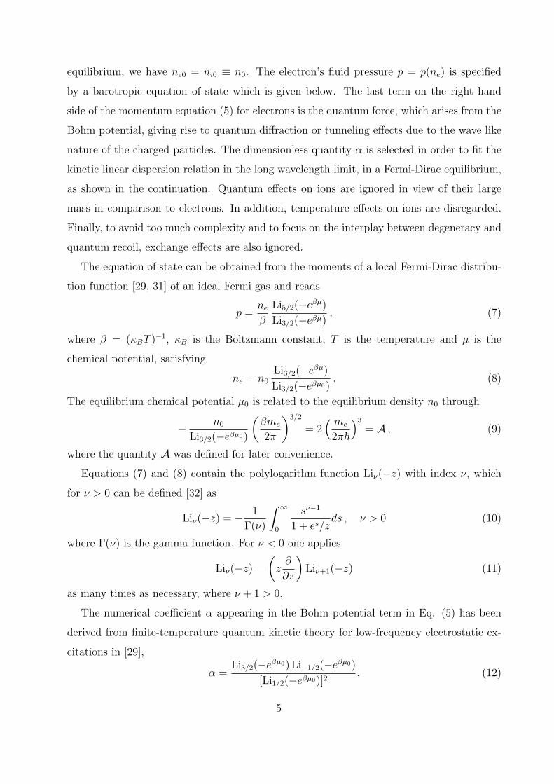
expressed as a function of the equilibrium fugacity z = exp(βµ0). The treatment of [29]
considered non-magnetized plasmas, but in Section V it is proved that Eq. (12) applies to
MIAWs too. As discussed in [29], in the classical limit (z ≪ 1) one has α ≈ 1, while in the
full degenerate limit (z ≫ 1) one has α ≈ 1/3. The same behavior is seen for α as a function
of the chemical potential, as depicted in Fig. 1, showing a transition zone from classical to
dense regimes.
Α = 1 3
-2 0 2 4
0.2
0.4
0.6
0.8
1
Μ0HeVL
Α
FIG. 1: Coefficient α from Eq. (12), as a function of the chemical potential µ0. Solid line:
T = 4000K. Doted line: T = 6000K. Dashed line: T = 8000K.
It happens [33] that the finite-temperature quantum hydrodynamic equations using α
from Eq. (12) are consistent with the results from orbital free density functional theory
[34, 35].
III. LINEAR WAVES
In order to find the dispersion relation for electrostatic wave in a magnetized quantum
plasma with arbitrary degeneracy of electrons, we linearize the system of equations (1)-(6)
by considering
ni = n0 + ni1 , ne = n0 + ne1 , uix = uix1 ,
uiy = uiy1 , uiz = uiz1 , ϕ = ϕ1 , (13)
6
Page 7
inducing a correction µ = µ0 + µ1, where the subscript 1 denotes the first order quantities.
In particular, using the expansion of the polylogarithm function to first order, i.e.,
Liν(−eβ(µ0+µ1)) = Liν(−eβµ0) + βµ1Liν−1(−eβµ0) , (14)
and considering plane wave perturbations ∼ exp[i(kxx+ kyy − ωt)], the result is
1 + χi(ω,k) + χe(0,k) = 0 , (15)
where the ionic and electronic susceptibilities are respectively given by
χi(ω,k) = −ω2pi(ω
2 − ω2ci cos
2 θ)
ω2(ω2 − ω2ci)
, (16)
χe(0,k) = ω2pe
[1
me
(dp
dne
)0
k2 +α~2k4
12m2e
]−1
, (17)
where ω2pj = n0e
2/(mjε0) for j = i, e and k = k (cos θ, sin θ, 0). Due to the neglect of
electrons inertia, only the static electronic susceptibility χe(0,k) is necessary. There is no
loss of generality in assuming waves in the xy plane, due to the cylindrical geometry around
the x−axis.
The dispersion relation (15) develops as a quadratic equation for ω2 whose solution is
ω2 =1
2
[ω20 + ω2
ci (18)
±((ω2
0 + ω2ci)
2 − 4ω20ω
2ci cos
2 θ)1/2]
,
where ω0 was already obtained [29] in the case of unmagnetized quantum ion-acoustic waves,
ω20 =
c2sk2 [1 +H2(kλD)
2/4]
1 + (kλD)2 +H2(kλD)4/4. (19)
In Eq. (19) one has the ion-acoustic speed cs which follows from
c2s =1
mi
(dp
dne
)0
=κBT
mi
Li3/2(−eβµ0)
Li1/2(−eβµ0), (20)
the generalized electronic screening length λD from
λ2D =
c2sω2pi
=κBT
meω2pe
Li3/2(−eβµ0)
Li1/2(−eβµ0), (21)
as well as the quantum diffraction parameter H specified by
H =β~ωpe√
3
(Li−1/2(−eβµ0)
Li3/2(−eβµ0)
)1/2
. (22)
7
Page 8
In the dilute plasma limit eβµ0 ≪ 1, implying Liν(−eβµ0) ≈ −eβµ0 , one has cs ≈√κBT/mi, λD =
√κBT/(meω2
pe), which respectively are the more traditional ion-acoustic
speed and Debye length, and H ≈ β~ωpe/√3. On the other hand, in the fully degenerate
case eβµ0 ≫ 1, using Liν(−eβµ0) ≈ −(βµ0)ν/Γ(ν+1) one has µ0 ≈ EF = ~2(3π2n0)
2/3/(2me),
which is the Fermi energy, and cs ≈√(2/3)EF/mi, λD =
√2EF/(3meω2
pe), which are re-
spectively the quantum ion-acoustic speed and the Thomas-Fermi screening length, and
H ≈ (1/2)~ωpe/EF . The dispersion relation (18) is formally the same as for classical mag-
netized plasma [36, 37], provided the fully quantum ion-acoustic frequency ω0 is replaced by
its purely classical counterpart.
As apparent from the dispersion relation (15), ions are responsible for providing inertia
effects, while electrons are responsible for kinetic energy (arising from the standard, ther-
modynamic temperature and/or Fermi pressure) and quantum diffraction is represented by
the parameter H. It is convenient to rewrite Eq. (22) using Eq. (9), yielding
H2 = −2αF
3
√2βmec2
πLi−1/2(−eβµ0) , (23)
where αF = e2/(4πε0~c) ≈ 1/137 is the fine structure constant. Obviously the theory is
non-relativistic, in spite of the appearance of the rest energy mec2 in Eq. (23).
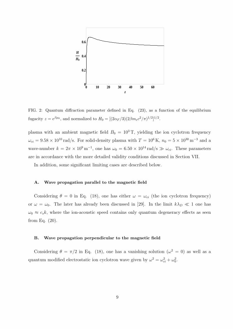
For a fixed temperature, H is a simple function of the fugacity z = exp(βµ0), as shown
in Fig. 2 below. It is seen that the pure wave like quantum effects are enhanced for
larger densities (and fugacities) up to z ≈ 3.03, while for larger degeneracy the quantum
statistical effects prevail showing that the quantum force becomes less effective in denser
systems, in view of Pauli’s exclusion principle. Therefore for dilute systems H increases
with the density and decreases with temperature, while for fully degenerate systems the
leading order behavior shows a decreasing of H for an increasing density.
The positive sign in Eq. (18) corresponds to fast electrostatic waves, and a negative sign
corresponds to slow electrostatic waves in a magnetized plasma. The effect of degeneracy
for arbitrary angle θ is not entirely straightforward to identify, due to the somehow involved
expression (18). However, in practical applications it is likely to have ω0 ≫ ωci, so that
the fast mode becomes ω2 ≈ ω20 + ω2
ci sin2 θ while the slow mode becomes ω2 ≈ ω2
ci cos2 θ.
Since quantum effects are present only on ω20 ≫ ω2
ci, it happens that the fast wave has
an angular dependence appearing as a correction, while the slow wave is strongly angle
dependent, but not so influenced by quantum effects. As an example, consider hydrogen
8
Page 9
0 10 20 30 40 50 600
0.2
0.4
0.6
z
H
H0
FIG. 2: Quantum diffraction parameter defined in Eq. (23), as a function of the equilibrium
fugacity z = eβµ0 , and normalized to H0 = [(2αF /3)(2βmec2/π)1/2]1/2.
plasma with an ambient magnetic field B0 = 103 T, yielding the ion cyclotron frequency
ωci = 9.58× 10¹⁰ rad/s. For solid-density plasma with T = 106 K, n0 = 5× 1030 m−3 and a
wave-number k = 2π × 109m−1, one has ω0 = 6.50 × 10¹⁴ rad/s ≫ ωci. These parameters
are in accordance with the more detailed validity conditions discussed in Section VII.
In addition, some significant limiting cases are described below.
A. Wave propagation parallel to the magnetic field
Considering θ = 0 in Eq. (18), one has either ω = ωci (the ion cyclotron frequency)
or ω = ω0. The later has already been discussed in [29]. In the limit kλD ≪ 1 one has
ω0 ≈ csk, where the ion-acoustic speed contains only quantum degeneracy effects as seen
from Eq. (20).
B. Wave propagation perpendicular to the magnetic field
Considering θ = π/2 in Eq. (18), one has a vanishing solution (ω2 = 0) as well as a
quantum modified electrostatic ion cyclotron wave given by ω2 = ω2ci + ω2
0.
9
Page 10
C. Strongly magnetized ions
For completeness we consider the strongly magnetized ions case. If ωci ≫ ω0 one has the
fast mode
ω2 = ω2ci
[1 +
ω20
ω2ci
sin2 θ +ω40
4ω4ci
sin2(2θ) +O
((ω0
ωci
)6)]
, (24)
and the slow mode
ω2 = ω20 cos
2 θ
[1− ω2
0
ω2ci
sin2 θ +O
((ω0
ωci
)4)]
. (25)
IV. ELECTRON INERTIA AND MAGNETIZATION EFFECTS
In the purely classical case, the conditions of applicability of the model are well-known
[18, 19]. In the quantum case, it is interesting to include electron inertia and magnetization
effects, to measure the limitations of Eq. (15). In this context one adds to Eqs. (1)-(4) and
(6) the electron continuity equation
∂ne
∂t+
∂
∂x(neuex) +
∂
∂y(neuey) = 0 , (26)
and replace Eq. (5) by
me
(∂ue
∂t+ ue · ∇ue
)= −∇p
ne
− e(−∇ϕ+ ue ×B0
)+
α~2
6me
∇[ 1√ne
( ∂2
∂x2+
∂2
∂y2
)√ne
], (27)
where ue = (uex, uey, uez) is the electron fluid velocity. Proceeding as in Section III and also
supposing linear perturbations where ue = ue1, the result is
1 + χi(ω,k) + χe(ω,k) = 0 , (28)
where the ionic susceptibility is still given by Eq. (16) and
χe(ω,k) = −ω2pe(ω
2 − ω2ce cos
2 θ)
ω4 − (k2v2T (k) + ω2ce)ω
2 + k2v2T (k)ω2ce cos
2 θ, (29)
where ωce = eB0/me is the electron cyclotron frequency and
v2T (k) =1
me
(dp
dne
)0
+α~2k2
12m2e
. (30)
10
Page 11
It is not the purpose of this work to develop the full consequences of the dispersion relation
(28), but it is useful to observe that in the formal limit ω → 0 the electron response (29)
regains the static electronic response χe(0,k) given by Eq. (17). Moreover, by inspection
of Eq. (29) it is found that such a limit is attended for a warm electron fluid, where
k2v2T (k) ≫ ω2ce so that the electrons magnetization could be disregarded, and k2v2T (k) ≫ ω2,
which is attainable for low frequency excitations. In addition, notice that vT (k) from Eq.
(30) depends not only on pressure but also on quantum diffraction effects. On the other
hand, ions are assumed to be cold and non-quantum enough.
V. COMPARISON TO KINETIC THEORY
The results from hydrodynamics should agree with kinetic theory in the long wavelength
limit. Therefore it is necessary to compare the ionic and electronic responses found from
kinetic theory, to the susceptibilities shown in Eqs. (16) and (17). Since ions are safely
assumed as classical in most cases, their particle distribution function fi = fi(r,v, t) satisfy
Vlasov’s equation, which presently is[∂
∂t+ v · ∇+
e
mi
(−∇ϕ+ v ×B0) ·∂
∂v
]fi = 0 . (31)
On the other hand, the quantum nature of electrons deserves the use of the quantum
Vlasov equation satisfied by the electronic Wigner quasi-distribution fe = fe(r,v, t),
∂fe∂t
+ v · ∇fe −ie
~
( me
2π~
)3× (32)
×∫
ds dv′ exp
(ime(v
′ − v) · s~
)×
×[ϕ(r+
s
2, t)− ϕ
(r− s
2, t)]
fe(r,v′, t) = 0 .
All integrals run from −∞ to ∞, unless otherwise stated. Moreover, under the same as-
sumption as before, namely large electron thermal and quantum (statistical and diffraction)
effects, the magnetic force on electrons was omitted in Eq. (32).
The scalar potential is self-consistently determined by Poisson’s equation,(∂2
∂x2+
∂2
∂y2
)ϕ =
e
ε0
(∫fe dv −
∫fi dv
), (33)
where we are taking spatial variations in the xy-plane only.
11
Page 12
Proceeding as in Section III, assuming plane wave perturbations ∼ exp[i(kxx+kyy−ωt)]
around isotropic in velocities equilibria, the dispersion relation 1 + χi(ω,k) + χe(ω,k) = 0
is easily derived. Disregarding the negligibly small Landau damping of MIAWs in the case
of cold ions, it is found [38, 39] that the ionic susceptibility from kinetic theory coincides
with the fluid expression (16). On the other hand, for low frequency waves, the static limit
χe(0,k) is sufficient for electrons, reading
χe(0,k) =e2
ε0~k2
∫dv
k · v
[F
(v− ~k
2me
)− F
(v+
~k2me
)], (34)
where the principal value of the integral is understood if necessary and where the equilibrium
electronic Wigner function is fe = F (v).
Consider a Fermi-Dirac equilibrium,
F (v) =A
1 + eβ(mev2/2−µ0), v = |v| , (35)
where the normalization constant A is given in Eq. (9), assuring that∫F (v) dv = n0.
It turns out that the right-hand side of Eq. (34) can be evaluated as a power series of the
quantum recoil q =√
β/(2me) ~k/2, supposed to be a small quantity for long wavelengths
and/or sufficiently large electronic temperature:
χe(0,k) =βmeω
2pe√
π Li3/2(−z)k2
[Γ
(1
2
)Li1/2(−z) +
+ Γ
(−1
2
)Li−1/2(−z)
q2
3
+ Γ
(−3
2
)Li−3/2(−z)
q4
5+ . . .
]=
βmeω2pe√
π Li3/2(−z)k2
∞∑j=0
Γ
(1
2− j
)×
× Li1/2−j(−z)q2j
2j + 1, (36)
where z = eβµ0 . The derivation is detailed in the Appendix A. The expression (36) is exact,
as long as the series converges. Moreover, it coincides with the static limit of Eq. (29) of
[40], where only the leading O(q2) quantum recoil correction was calculated.
12
Page 13
For the sake of comparison, the hydrodynamic result from Eq. (17) can be rewritten as
χe(0,k) =βmeω
2peLi1/2(−z)
Li3/2(−z)k2
(1 +
2q2
3
Li−1/2(−z)
Li1/2(−z)
)−1
=βmeω
2pe
Li3/2(−z)k2
(Li1/2(−z)− 2q2
3Li−1/2(−z)
+ O(q4)), (37)
which coincides with Eq. (36) in the long wavelength limit, in view of Γ(1/2) =√π, Γ(−1/2) = −2
√π. This completes the justification of α in Eq. (12) in the magnetized
case.
VI. ZAKHAROV-KUZNETSOV EQUATION FOR ARBITRARY DEGENERACY
In order to derive the ZK equation for obliquely propagating MIAWs in arbitrary de-
generate plasma, it is convenient to make use of normalized quantities. The dispersion
relation (18) suggests the use of the dimensionless variables (x, y) = (x, y)/λD, t = ωpit,
(uix, uiy, uiz) = (uix, uiy, uiz)/cs as well as ϕ = eϕ/(mic2s), nj = nj/n0, where j = e, i.
Equations (1)-(6) are then written as
∂ni
∂t+
∂
∂x(niuix) +
∂
∂y(niuiy) = 0 , (38)
∂uix
∂t+
(uix
∂
∂x+ uiy
∂
∂y
)uix = −∂ϕ
∂x, (39)
∂uiy
∂t+
(uix
∂
∂x+ uiy
∂
∂y
)uiy = −∂ϕ
∂y+ Ωuiz , (40)
∂uiz
∂t+
(uix
∂
∂x+ uiy
∂
∂y
)uiz = −Ωuiy , (41)
0 = ∇ϕ−Li1/2(−eβµ0)
Li1/2(−eβµ)∇ne
+H2
2∇[
1√ne
(∂2
∂x2+
∂2
∂y2
)√ne
], (42)(
∂2
∂x2+
∂2
∂y2
)ϕ = ne − ni , (43)
where Ω = ωci/ωpi has been defined and where ∇ = (∂/∂x, ∂/∂y, 0), while Eq. (8) becomes
ne =Li3/2(−eβµ)
Li3/2(−eβµ0). (44)
13
Page 14
In the following calculations, for brevity the tilde sign used for defining normalized quantities
will be omitted.
In order to find a nonlinear evolution equation describing the magnetized plasma, the
stretching of the independent variables x, y and t is defined under the assumption of strong
magnetization as follows [41–44],
X = ε1/2(x− V0t) , Y = ε1/2y , τ = ε3/2t , (45)
where ε is a formal small expansion parameter and V0 is the phase velocity of the wave, to
be determined later on. The perturbed quantities can be expanded in powers of ε as follows,
nj = 1 + εnj1 + ε2nj2 + ... , j = e, i , (46)
uix = εux1 + ε2ux2 + ε3ux3... , (47)
ui⊥ = ε3/2u⊥1 + ε2u⊥2 + ε5/2u⊥3... , ⊥= y, z , (48)
ϕ = εϕ1 + ε2ϕ2 + ... , (49)
µ = µ0 + εµ1 + ε2µ2 + ... (50)
In the present model, the ion velocity components (uiy, uiz) in the perpendicular to the
magnetic field directions are taken as higher order perturbations compared to the parallel
component uix since in the presence of a strong magnetic field, the plasma is anisotropic so
that the ion gyro-motion becomes a higher order effect.
The lowest ε order terms (∼ ε3/2) from the set of equations (38)-(42) give
−V0∂ni1
∂X+
∂ux1
∂X= 0 , (51)
V0∂ux1
∂X=
∂ϕ1
∂X, (52)
uz1 =1
Ω
∂ϕ1
∂Y, (53)
−Ωuy1 = 0 , (54)
∂ϕ1
∂X=
∂ne1
∂X. (55)
The velocity uz1 appears in Eq. (53) due to the E ×B drift.
The lowest ε order terms (∼ ε) from equations (43) and (44) give
ni1 = ne1 =Li1/2(−eβµ0)
Li3/2(−eβµ0)βµ1 . (56)
14
Page 15
Solving the system (51)-(56), we get V0 = ±1. We set V0 = 1 (the normalized phase velocity
of the MIAW) without loss of generality.
Collecting the next higher order terms of the ion continuity (∼ ε5/2) and of the X , Y and
Z components of the ion momentum equations (∼ ε5/2, ε2, ε2), and after a rearrangement,
we find
∂ni1
∂τ− ∂ni2
∂X+
∂ux2
∂X+
∂
∂X(ni1ux1) +
∂uy2
∂Y= 0 , (57)
∂ux1
∂τ− ∂ux2
∂X+ ux1
∂
∂Xux1 = −∂ϕ2
∂X, (58)
−∂uy1
∂X= Ωuz2 , (59)
∂uz1
∂X= Ωuy2 . (60)
Using Eq. (56) and the next higher order terms ∼ ε5/2 from the equations of motion of the
inertialess degenerate electrons in the X and Y directions, we get
∂ne2
∂X=
∂ϕ2
∂X+ αne1
∂ne1
∂X+
H2
4
(∂3
∂X3+
∂
∂X
∂2
∂Y 2
)ne1 (61)
and∂ne2
∂Y=
∂ϕ2
∂Y+ αne1
∂ne1
∂Y+
H2
4
(∂
∂Y
∂2
∂X2+
∂3
∂Y 3
)ne1, (62)
where α has been defined in equation (12).
Now collecting the ε2 order terms from Poisson’s equation, we have(∂2
∂X2+
∂2
∂Y 2
)ϕ1 = ne2 − ni2 , (63)
while the next higher terms from Eqs. (57), (58) and (60) give
∂ni2
∂X=
∂ni1
∂τ+
∂
∂X(ni1ux1) +
1
Ω
∂
∂Y
(∂uz1
∂X
)+∂ux1
∂τ+ ux1
∂ux1
∂X+
∂ϕ2
∂X. (64)
Differentiating Eq. (63) with respect to X and using Eqs. (61) and (64) together with
ni1 = ne1 = ux1 = ϕ1, uz1 = (1/Ω) ∂ϕ1/∂Y , it is finally possible to write the ZK equation
for obliquely propagating quantum MIAWs in terms of ϕ1 ≡ φ,
∂φ
∂τ+ Aφ
∂φ
∂X+
∂
∂X
(B
∂2φ
∂X2+ C
∂2φ
∂Y 2
)= 0 . (65)
15
Page 16
The nonlinearity coefficient A and the dispersion coefficients B and C in the parallel and
perpendicular directions of the magnetic field, respectively, are defined as
A =1
2(3− α) , (66)
B =1
2
(1− H2
4
), (67)
C =1
2
(1 +
1
Ω2− H2
4
). (68)
In the purely classical limit the nonlinearity and dispersion coefficients become A = 1,
B = 1/2 and C = (1/2) (1 + 1/Ω2) in agreement with Refs. [17, 43, 44] treating MIAWs
in a classical electron-ion plasma. In addition, the ZK equation for fully degenerate plasma
will have A = 4/3 and H = (1/2) ~ωpe/EF in the coefficients B,C. The associated fully
degenerate ZK equation does not matches the results from Refs. [20–22], after comparison
using physical (dimensional and non-stretched) coordinates, restricted to the case of electron-
ion plasmas. Note that the ZK equations from the previous works do not match the purely
classical result.
Provided l2xB + l2yC = 0, the soliton solution of the ZK equation (65) for obliquely
propagating MIAWs is given by
φ = φ0 sech2(η/W ) , (69)
where φ0 = 3u0/(Alx) is the height and where W =√4lx(l2xB + l2yC)/u0 is the width
of the soliton in terms of the stretched coordinates. The polarity of the soliton depends
on the sign of φ0. The transformed coordinate η in the co-moving frame is defined as
η = lxX + lyY − u0τ , where u0 = 0 is the speed of the nonlinear pulse and where lx > 0
and ly are direction cosines, so that l2x + l2y = 1. To obtain localized structures, decaying
boundary conditions as η → ±∞ were applied. Following the habitual usage the terminology
“soliton” is applied to the solitary wave (69), although the ZK equation does not belong to
the class of completely integrable evolution equations. The dispersion effects arising from
the combination of charge separation and finite ion Larmor radius balances the nonlinearity
in the system to form the soliton.
Defining δV = εu0/lx, in the laboratory frame the solution reads
φ =3 δV
Asech2
12
(δV
l2xB + l2yC
)1/2
×
×[lx
(x− (V0 + δV ) t
)+ lyy
]. (70)
16
Page 17
It is apparent that V0 + δV corresponds to the velocity at which travels the intersection
between a plane of constant phase and a field line, down the same field line [42].
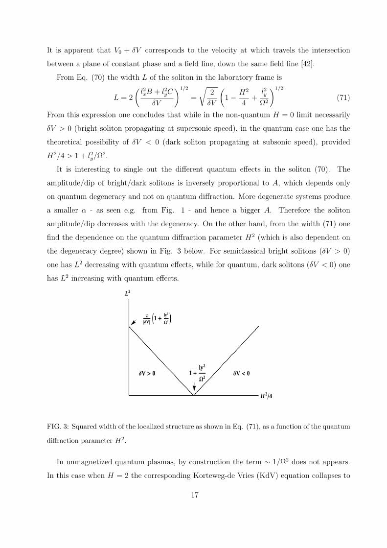
From Eq. (70) the width L of the soliton in the laboratory frame is
L = 2
(l2xB + l2yC
δV
)1/2
=
√2
δV
(1− H2
4+
l2yΩ2
)1/2
(71)
From this expression one concludes that while in the non-quantum H = 0 limit necessarily
δV > 0 (bright soliton propagating at supersonic speed), in the quantum case one has the
theoretical possibility of δV < 0 (dark soliton propagating at subsonic speed), provided
H2/4 > 1 + l2y/Ω2.
It is interesting to single out the different quantum effects in the soliton (70). The
amplitude/dip of bright/dark solitons is inversely proportional to A, which depends only
on quantum degeneracy and not on quantum diffraction. More degenerate systems produce
a smaller α - as seen e.g. from Fig. 1 - and hence a bigger A. Therefore the soliton
amplitude/dip decreases with the degeneracy. On the other hand, from the width (71) one
find the dependence on the quantum diffraction parameter H2 (which is also dependent on
the degeneracy degree) shown in Fig. 3 below. For semiclassical bright solitons (δV > 0)
one has L2 decreasing with quantum effects, while for quantum, dark solitons (δV < 0) one
has L2 increasing with quantum effects.
2∆VJ1 + ly2
W2 N
1 +ly2
W2
∆V > 0 ∆V < 0
H24
L2
FIG. 3: Squared width of the localized structure as shown in Eq. (71), as a function of the quantum
diffraction parameter H2.
In unmagnetized quantum plasmas, by construction the term ∼ 1/Ω2 does not appears.
In this case when H = 2 the corresponding Korteweg-de Vries (KdV) equation collapses to
17
Page 18
the Burger’s equation, producing an ion-acoustic shock wave structure instead of a soliton
[8].
In the magnetized case, a further possibility happens when C = 0, or, equivalently,
1 + 1/Ω2 = H2/4, which is not allowed in the classical limit (H ≡ 0). When C = 0, from
Eq. (65) one has∂φ
∂τ+ Aφ
∂φ
∂X− 1
2Ω2
∂3φ
∂X3= 0 , (72)
which transforms to the KdV equation in its standard form by means of φ → −φ,X →
−X, τ → τ . Therefore, in this particular situation the problem becomes completely inte-
grable.
Finally, if B = 0, it means that 1−H2/4 = 0 due to which C = 1/2Ω2, so that Eq. (65)
becomes∂φ
∂τ+ Aφ
∂φ
∂X+
1
2Ω2
∂
∂X
∂2φ
∂Y 2= 0, (73)
This is a KdV-like equation having perpendicular to the magnetic field dispersion effects,
due to the obliquely propagating MIAW.
Regarding the ranges of validity of the parameters A,B and C in Eqs. (66–68), first
we observe that from Eq. (12) one has 1/3 < α < 1, so that 1 < A < 4/3. In addition,
since H2 from Eq. (23) can in principle attain any non-negative value, B and C are not
positive definite. However, strictly speaking, very large values of H2 are associated with
strongly coupling effects which can have a large impact on soliton propagation, to be ad-
dressed in a separate extended theory. Only in such generalized framework one could be
able to make more precise statements on pure quantum soliton existence or non-existence.
Nevertheless, significant values of H2 are certainly physically acceptable, as found from the
present treatment. These issues are best discussed in the following Section.
VII. APPLICATIONS
It is important to discuss the validity domain of the general theory devised in the last
Sections. Moreover, it is highly desirable to offer precise physical parameters where the
predicted linear and nonlinear waves could be searched in practice. Obviously, the theory
is more relevant in the intermediate regimes, where the thermal and Fermi temperatures
are not significantly different. Otherwise, the fully degenerate or dilute limits could be
18
Page 19
sufficiently accurate. Therefore, in this Section frequently we assume
T = TF , (74)
where TF = EF/κB is the electrons Fermi temperature.
To start, consider the normalization condition (9), which can be expressed [26] as
Li3/2(−z) = − 4
3√π(βEF )
3/2 , (75)
where z = exp(βµ0). For equal thermal and Fermi temperatures, βEF = 1, which from
Eq. (75) gives the equilibrium fugacity z = 0.98 and from Eq. (12) a parameter α = 0.80,
definitely in the intermediate dilute-degenerate situation as explicitly seen e.g. in Fig. 1.
Besides quantum degeneracy, quantum diffraction effects can also provide qualitatively
new aspects as found e.g. in the extra dispersion of linear waves in Section III and the
modified width of the solitons in Section VI. Therefore it would be interesting to investigate
systems with a large parameter H. However, realistically speaking it is not possible to in-
crease H without limits, which would enter the strongly coupled plasma regime, not included
in the present formalism. For instance, the ideal Fermi gas equation of state for electrons
would be unappropriated. Therefore, it is necessary to analyze the coupling parameter g for
electrons, which can be defined [45] as g = l/a, where
l = − e2
12πε0κBT
n0Λ3T
Li5/2(−z)(76)
is a generalized Landau length involving the thermal de Broglie wavelength ΛT =
[2π~2/(meκBT )]1/2, and a = (4πn0/3)
−1/3 is the Wigner-Seitz radius. In the dilute case,
one has e2/(4πε0 l) = (3/2)κBT , so that l would be the classical distance of closest approach
in a binary collision, for average kinetic energy. The general expression (76) accounts for
the degeneracy effects on the mean kinetic energy. A few calculations yield
g = −2αF
√2βmec2
3 (3√π)1/3
[Li23/2(−z)]2/3
Li5/2(−z), (77)
an expression similar to the one for H2 in Eq. (23). Hence, it is legitimate to suspect that
the indiscriminate increase of quantum diffraction gives rise to nonideality effects such as
dynamical screening and bound states [45]. Incidentally Eq. (77) agrees with Eq. (16) of
[29], found from related but different methods.
19
Page 20
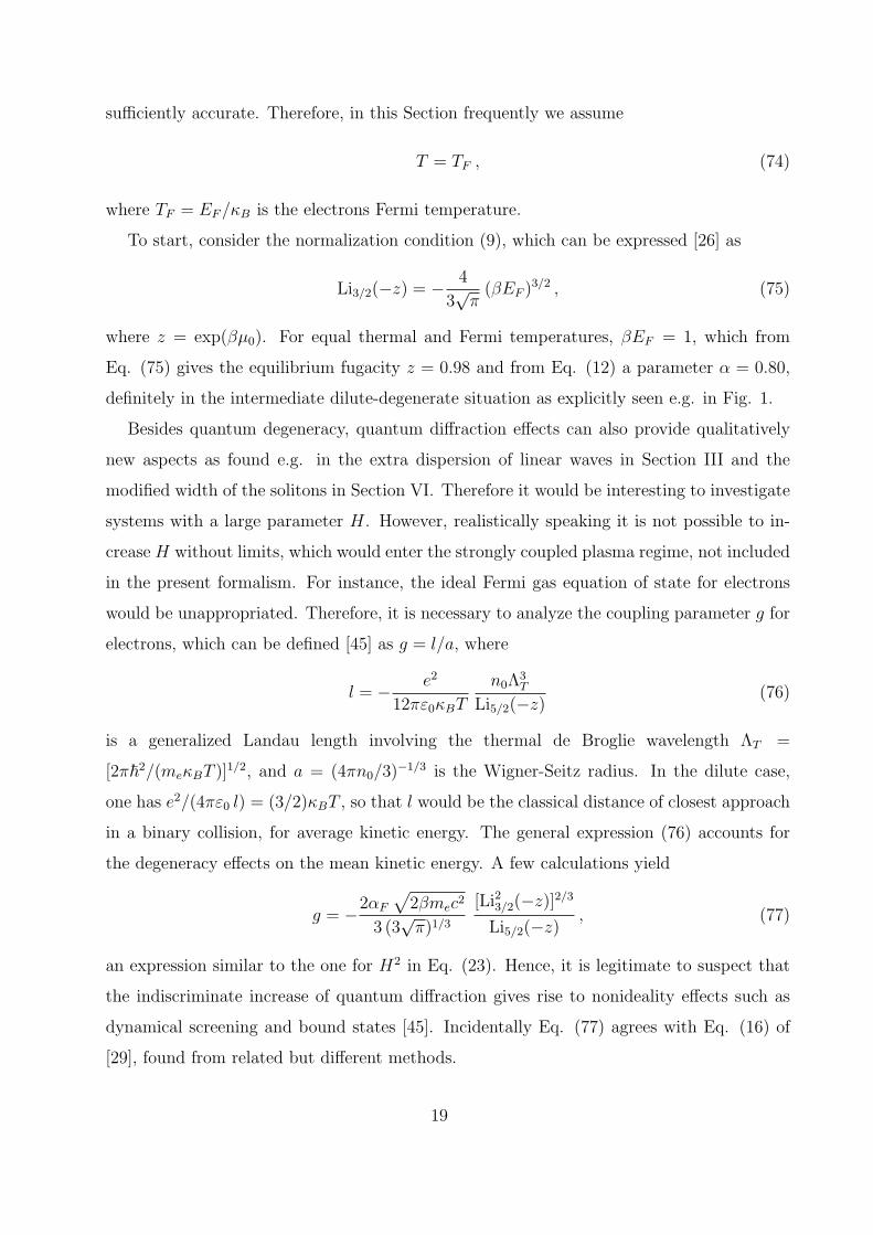
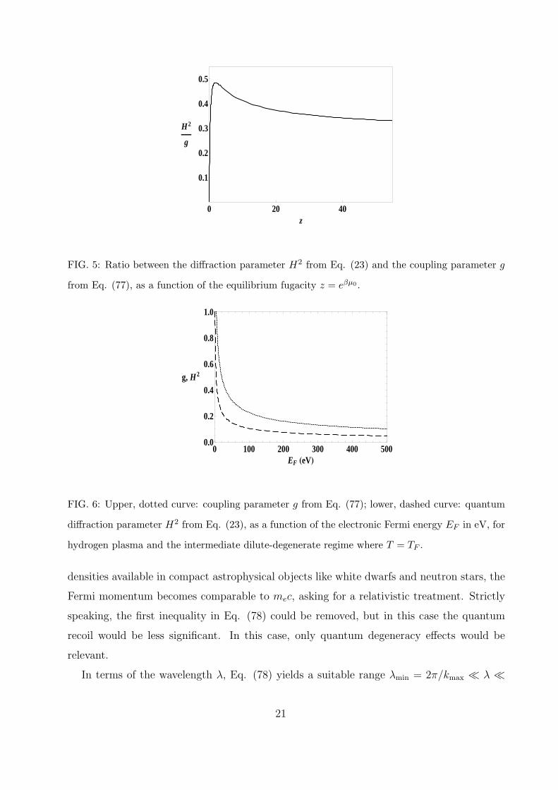
The resemblance between the coupling and quantum diffraction parameters is confirmed
in Fig. 4 below, which can be compared to Fig. 2 for H2. Moreover, it is apparent in
Fig. 5, that we have H2 < 0.5 for the whole span of degeneracy regimes, as far as g < 1.
Strictly speaking, the dark soliton, shock wave and the completely integrable case associated
to the KdV equation (72) are therefore outside the validity domain of the model, since they
need large values of quantum diffraction parameter H. Nevertheless, the influence of the
wave nature of the electrons can still provide important corrections by its own, at least for
reasonable values of H2, as is obvious, for instance, in the width of the ZK soliton in Eq.
(71).
0 10 20 30 40 50 60
0.2
0.4
0.6
0.8
z
g
g0
FIG. 4: Coupling parameter defined in Eq. (77), as a function of the equilibrium fugacity z = eβµ0 ,
and normalized to g0 = 2αF
√2βmec2/[3(3
√π)1/3].
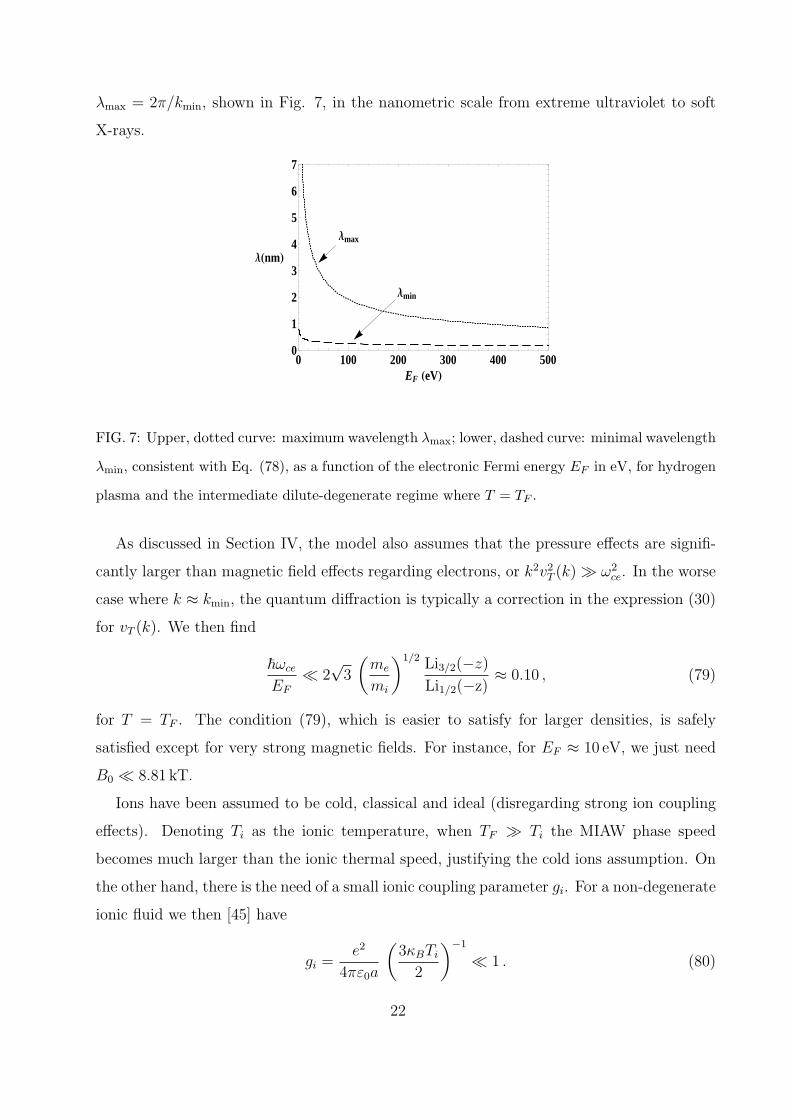
The behavior of the parameters g,H2 can be summarized in Fig. 6, for T = TF and
considering hydrogen plasma parameters. We observe that g < 1 for n0 > 5.23× 1028 m−3,
or EF > 5.11 eV, which starts becoming realizable for typical densities in solid-density
plasmas [46, 47].
It is necessary to discuss additional points about the validity conditions of the model.
Both the static electronic response and long wavelength (and hence fluid) assumptions are
collected in Eq. (27) of [29], reproduced here for convenience,
kmin ≡ 2√3mecs~
≪ k ≪ ωpi
cs≡ kmax . (78)
For hydrogen plasma and T = TF , from Eq. (78) one has kmax > kmin for n0 < 9.81 ×
1035m−3. The later condition is safely satisfied for non-relativistic plasma. At such high
20
Page 21
0 20 40
0.1
0.2
0.3
0.4
0.5
z
H2
g
FIG. 5: Ratio between the diffraction parameter H2 from Eq. (23) and the coupling parameter g
from Eq. (77), as a function of the equilibrium fugacity z = eβµ0 .
0 100 200 300 400 5000.0
0.2
0.4
0.6
0.8
1.0
EF HeVL
g, H2
FIG. 6: Upper, dotted curve: coupling parameter g from Eq. (77); lower, dashed curve: quantum
diffraction parameter H2 from Eq. (23), as a function of the electronic Fermi energy EF in eV, for
hydrogen plasma and the intermediate dilute-degenerate regime where T = TF .
densities available in compact astrophysical objects like white dwarfs and neutron stars, the
Fermi momentum becomes comparable to mec, asking for a relativistic treatment. Strictly
speaking, the first inequality in Eq. (78) could be removed, but in this case the quantum
recoil would be less significant. In this case, only quantum degeneracy effects would be
relevant.
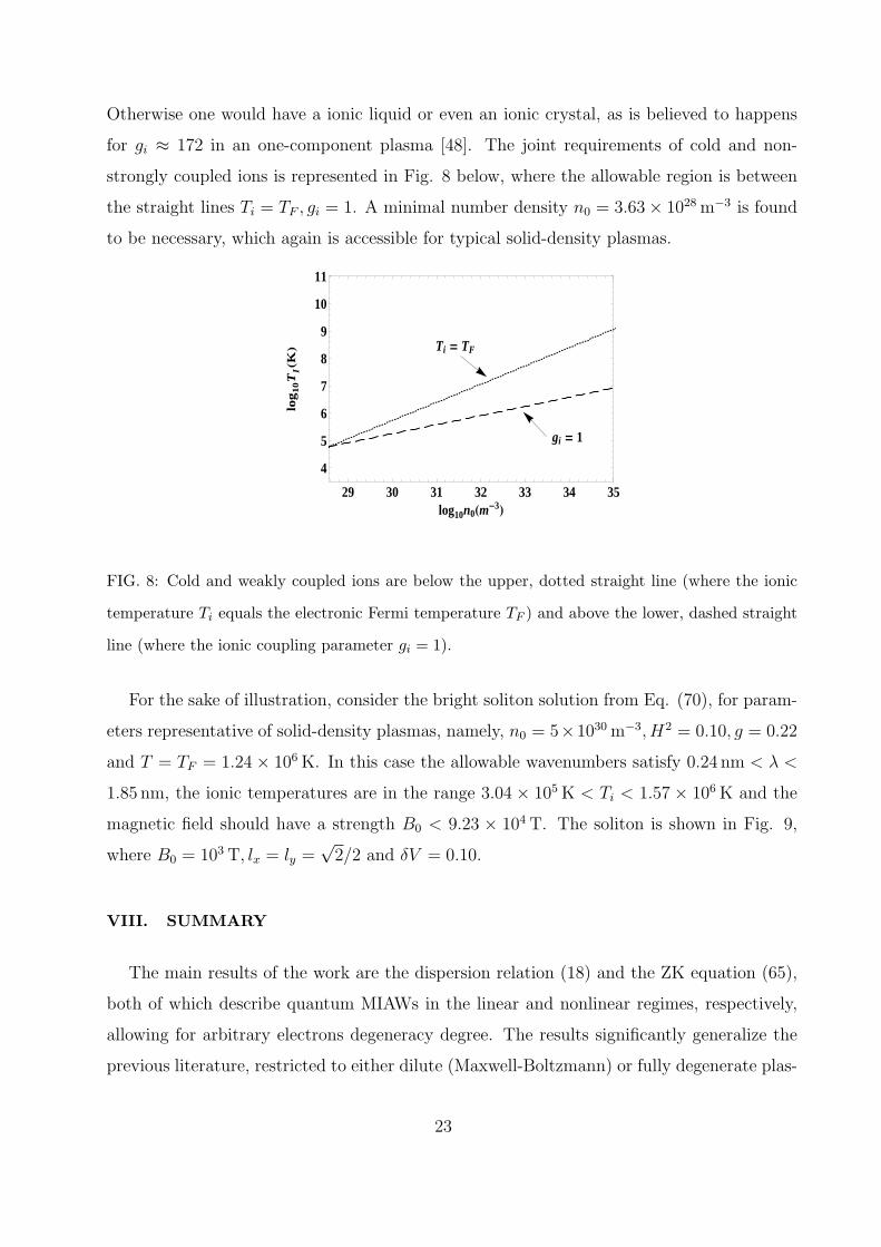
In terms of the wavelength λ, Eq. (78) yields a suitable range λmin = 2π/kmax ≪ λ ≪
21
Page 22
λmax = 2π/kmin, shown in Fig. 7, in the nanometric scale from extreme ultraviolet to soft
X-rays.
Λmax
Λmin
0 100 200 300 400 5000
1
2
3
4
5
6
7
EF HeVL
ΛHnmL
FIG. 7: Upper, dotted curve: maximum wavelength λmax; lower, dashed curve: minimal wavelength
λmin, consistent with Eq. (78), as a function of the electronic Fermi energy EF in eV, for hydrogen
plasma and the intermediate dilute-degenerate regime where T = TF .
As discussed in Section IV, the model also assumes that the pressure effects are signifi-
cantly larger than magnetic field effects regarding electrons, or k2v2T (k) ≫ ω2ce. In the worse
case where k ≈ kmin, the quantum diffraction is typically a correction in the expression (30)
for vT (k). We then find
~ωce
EF
≪ 2√3
(me
mi
)1/2 Li3/2(−z)
Li1/2(−z)≈ 0.10 , (79)
for T = TF . The condition (79), which is easier to satisfy for larger densities, is safely
satisfied except for very strong magnetic fields. For instance, for EF ≈ 10 eV, we just need
B0 ≪ 8.81 kT.
Ions have been assumed to be cold, classical and ideal (disregarding strong ion coupling
effects). Denoting Ti as the ionic temperature, when TF ≫ Ti the MIAW phase speed
becomes much larger than the ionic thermal speed, justifying the cold ions assumption. On
the other hand, there is the need of a small ionic coupling parameter gi. For a non-degenerate
ionic fluid we then [45] have
gi =e2
4πε0a
(3κBTi
2
)−1
≪ 1 . (80)
22
Page 23
Otherwise one would have a ionic liquid or even an ionic crystal, as is believed to happens
for gi ≈ 172 in an one-component plasma [48]. The joint requirements of cold and non-
strongly coupled ions is represented in Fig. 8 below, where the allowable region is between
the straight lines Ti = TF , gi = 1. A minimal number density n0 = 3.63× 1028 m−3 is found
to be necessary, which again is accessible for typical solid-density plasmas.
Ti = TF
gi = 1
29 30 31 32 33 34 35
4
5
6
7
8
9
10
11
log10n0Hm-3L
log
10T
IHKL
FIG. 8: Cold and weakly coupled ions are below the upper, dotted straight line (where the ionic
temperature Ti equals the electronic Fermi temperature TF ) and above the lower, dashed straight
line (where the ionic coupling parameter gi = 1).
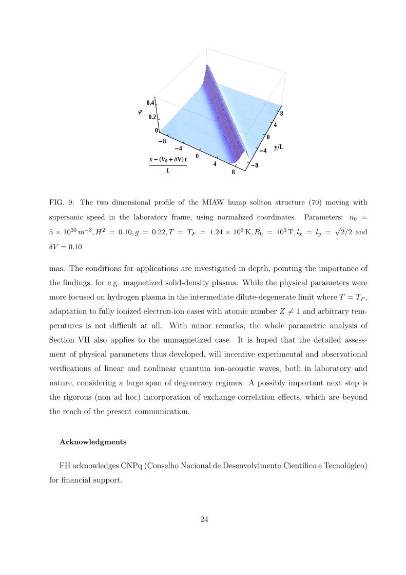
For the sake of illustration, consider the bright soliton solution from Eq. (70), for param-
eters representative of solid-density plasmas, namely, n0 = 5×1030 m−3, H2 = 0.10, g = 0.22
and T = TF = 1.24× 10⁶K. In this case the allowable wavenumbers satisfy 0.24 nm < λ <
1.85 nm, the ionic temperatures are in the range 3.04 × 10⁵K < Ti < 1.57 × 10⁶ K and the
magnetic field should have a strength B0 < 9.23 × 10⁴ T. The soliton is shown in Fig. 9,
where B0 = 103 T, lx = ly =√2/2 and δV = 0.10.
VIII. SUMMARY
The main results of the work are the dispersion relation (18) and the ZK equation (65),
both of which describe quantum MIAWs in the linear and nonlinear regimes, respectively,
allowing for arbitrary electrons degeneracy degree. The results significantly generalize the
previous literature, restricted to either dilute (Maxwell-Boltzmann) or fully degenerate plas-
23
Page 24
-8-4
04
8
x - HV0 + ∆VL t
L-8
-4
0
4
8
yL
0
0.2
0.4j
FIG. 9: The two dimensional profile of the MIAW hump soliton structure (70) moving with
supersonic speed in the laboratory frame, using normalized coordinates. Parameters: n0 =
5 × 1030m−3,H2 = 0.10, g = 0.22, T = TF = 1.24 × 10⁶K, B0 = 103T, lx = ly =√2/2 and
δV = 0.10
mas. The conditions for applications are investigated in depth, pointing the importance of
the findings, for e.g. magnetized solid-density plasma. While the physical parameters were
more focused on hydrogen plasma in the intermediate dilute-degenerate limit where T = TF ,
adaptation to fully ionized electron-ion cases with atomic number Z = 1 and arbitrary tem-
peratures is not difficult at all. With minor remarks, the whole parametric analysis of
Section VII also applies to the unmagnetized case. It is hoped that the detailed assess-
ment of physical parameters thus developed, will incentive experimental and observational
verifications of linear and nonlinear quantum ion-acoustic waves, both in laboratory and
nature, considering a large span of degeneracy regimes. A possibly important next step is
the rigorous (non ad hoc) incorporation of exchange-correlation effects, which are beyond
the reach of the present communication.
Acknowledgments
FH acknowledges CNPq (Conselho Nacional de Desenvolvimento Cientıfico e Tecnologico)
for financial support.
24
Page 25
APPENDIX A: DERIVATION OF EQ. (36)
From Eqs. (34) and (35) one has
χe(0,k)
=Ae2
ε0~k2
∫dv
[1
k · v + ~k2/(2me)− 1
k · v − ~k2/(2me)
]×
× 1
1 + exp(βmev2/2)/z
=2πAe2
ε0~k2
∫ ∞
−∞dv∥
[1
kv∥ + ~k2/(2me)− 1
kv∥ − ~k2/(2me)
]×
×∫ ∞
0
dv⊥v⊥
1 + exp[βme(v2⊥ + v2∥)/2]/z, (A1)
where v = v∥k/k + v⊥ ,k · v⊥ = 0, z = exp(βµ0) and all integrals consider the principal
value sense.
Performing the v⊥ integral, considering the expression of A in Eq. (9) and applying a
simple change of variables we get
χe(0,k) =βmeω
2pe
4√π Li3/2(−z)qk2
∫ ∞
−∞
ds
s× (A2)
×[ln(1 + ze−(s+q)2
)− ln
(1 + ze−(s−q)2
)],
where q =√
β/(2me) ~k/2.
Expanding in powers of the quantum recoil one has
ln(1 + ze−(s+q)2
)− ln
(1 + ze−(s−q)2
)(A3)
= −4q(g(s) +
q2
3!g′′(s) +
q4
5!g(iv)(s) +O(q6)
),
where g(s) ≡ s/[1 + exp(s2)/z]. At this point notice that the possible divergence at s = 0
in the integral (A2) was explicitly removed.
After integrating by parts, it is found that
χe(0,k) = −2βmeω
2pez√
π Li3/2(−z)k2
(∫ ∞
0
ds
z + es2
− 2q2
3
∫ ∞
0
ds es2
(z + es2)2(A4)
+4q4
15
∫ ∞
0
ds es2(es
2 − z)
(z + es2)3+O(q6)
).
25
Page 26
From Eqs. (10) and (11), each term on the right hand side of (A4) can be evaluated in terms
of polylogarithms. For instance,
Li1/2(−z) = − 2z√π
∫ ∞
0
ds
z + es2,
Li−1/2(−z) = − 2z√π
∫ ∞
0
ds es2
(z + es2)2, (A5)
Li−3/2(−z) =2z√π
∫ ∞
0
ds es2(z − es
2)
(z + es2)3,
clearly related to the integrals in expression (A4). In this way Eq. (36), which is also
independently confirmed by numerical evaluation, is proved.
[1] P. A. Markowich, C. A. Ringhofer and C. Schmeiser, Semiconductor Equations (Springer-
Verlag, Vienna, 1990).
[2] M. Marklund and P.K. Shukla, Rev. Mod. Phys. 78, 591 (2006).
[3] S. H. Glenzer, O. L. Landen, P. Neumayer, R. W. Lee, K. Widmann, S. W. Pollaine, R.
J. Wallace, G. Gregori, A. Holl, T. Bornath, R. Thiele, V. Schwarz, W.-D. Kraeft and R.
Redmer, Phys. Rev. Lett. 98, 065002 (2007).
[4] J. E. Cross, B. Reville and G. Gregori, Astrophys. J. 795, 59 (2014).
[5] M. Opher, L. O. Silva, D. E. Dauger, V. K. Decyk and J. M. Dawson, Phys. Plasmas 8, 2454
(2001).
[6] G. Chabrier, D. Saumon and A. Y. Potekhin, J. Phys. A: Math. Gen. 39, 4411 (2006).
[7] A. K. Harding and D. Lai, Rep. Prog. Phys. 69, 2631 (2006).
[8] F. Haas, L. G. Garcia, J. Goedert and G. Manfredi, Phys. Plasmas 10, 3858 (2003).
[9] F. Haas, Quantum Plasmas: an Hydrodynamic Approach (Springer, New York, 2011).
[10] R. E. Wyatt, Quantum Dynamics with Trajectories: Introduction to Quantum Hydrodynamics
(Springer, New York, 2005).
[11] P. K. Shukla and B. Eliasson, Physics-Uspekhi 53, 51 (2010).
[12] F. Haas, Phys. Plasmas 12, 062117 (2005).
[13] H. Tercas, J. T. Mendonca and P. K. Shukla, Phys. Plasmas 15, 072109 (2008).
[14] J. Zamanian, M. Marklund and G. Brodin, Phys. Rev. E 88, 063105 (2013).
[15] J. Zamanian, M. Marklund and G. Brodin, Eur. Phys. J. D 69, 25 (2015).
26
Page 27
[16] R. Ekman, J. Zamanian and G. Brodin, Phys. Rev. E 92, 013104 (2015).
[17] V. Zakharov and E. Kuznetsov, Sov. Phys. JETP 39, 285 (1974).
[18] E. Infeld and G. Rowlands, Nonlinear Waves, Solitons and Chaos (Cambridge University
Press, Cambridge, 2000)
[19] E. W. Laedke and K. H. Spatschek, Phys. Rev. Lett. 47, 719 (1981).
[20] R. Sabry, W. M. Moslem, F. Haas. S. Ali and P.K. Shukla, Phys. Plasmas 15, 122308 (2008).
[21] W. M. Moslem, S. Ali, P. K. Shukla, X. Y. Tang and G. Rowlands, Phys. Plasmas 14, 082308
(2007).
[22] S. A. Khan and W. Masood, Phys. Plasmas 15, 062301 (2008).
[23] N. Maafa, Phys. Scripta 48, 351 (1993).
[24] A. E. Dubinov, A. A. Dubinova and M. A. Sazokin, J. Commun. Tech. Elec. 55, 907 (2010).
[25] A. E. Dubinov and I. N. Kitaev, Phys. Plasmas 21, 102105 (2014).
[26] B. Eliasson and P. K. Shukla, Phys. Scripta 78, 025503 (2008).
[27] M. McKerr, F. Haas and I. Kourakis, Phys. Rev. E 90, 033112 (2014).
[28] E. E. Behery, F. Haas and I. Kourakis, Phys Rev. E 93, 023206 (2016).
[29] F. Haas and S. Mahmood, Phys. Rev. E 92, 053112 (2015).
[30] V. E. Fortov, Extreme States of Matter on Earth and in the Cosmos (Springer, Berlin, 2011).
[31] R. K. Pathria and P. D. Beale, Statistical Mechanics-3rd Edition (Elsevier, New York USA,
2011).
[32] L. Lewin, Polylogarithms and Associated Functions (North Holland, New York, 1981).
[33] B. Eliasson and M. Akbari-Moghanjoughi, Finite temperature static charge scree-
ning in quantum plasmas, accepted for publication in Phys. Lett. A (2016), DOI
10.1016/j.physleta.2016.05.043 .
[34] L. G. Stanton and M. S. Murillo, Phys. Rev. E 91, 033104 (2015).
[35] L. G. Stanton, M. S. Murillo, Phys. Rev. E 91, 049901(E) (2015).
[36] T. E. Stringer, J. Nucl. Energy Part C 5, 89 (1963).
[37] E. Witt and W. Lotko, Phys. Fluids 26, 2176 (1983).
[38] K. N. Stepanov, Soviet Phys. JETP 8, 808 (1959).
[39] A. I. Akhiezer, I. A. Akhiezer, R. V. Polovin, A. G. Sitenko and K. N. Stepanov, Plasma
Electrodynamics - vol. I (Pergamon, Oxford, 1975).
[40] D. B. Melrose and A. Mushtaq, Phys. Rev. E 82, 056402 (2010).
27
Page 28
[41] I. Kourakis, W. M. Moslem, U. M. Abdelsalam, R. Sabry and P. K. Shukla, Plasma Fusion
Res. 4, 018 (2009).
[42] R. L. Mace and M. A. Hellberg, Phys. Plasmas 8, 2649 (2001).
[43] E. Infeld, J. Plasma Phys. 33, 171 (1985).
[44] E. W. Laedke and K. H. Spatschek, Phys. Fluids 25, 985 (1982).
[45] D. Kremp, M. Schlanges andW.-D. Kraeft, Quantum Statistics of Nonideal Plasmas (Springer-
Verlag, Berlin-Heidelberg, 2005).
[46] M. Tatarakis, I. Watts, F. N. Beg, E. L. Clark, A. E. Dangor, A. Gopal, M. G. Haines, P. A.
Norreys, U. Wagner, M.-S. Wei, M. Zepf and K. Krushelnick, Nature 415, 280 (2002).
[47] U. Wagner, M. Tatarakis, A. Gopal, F. N. Beg, E. L. Clark, A. E. Dangor, R. G. Evans, M.
G. Haines, S. P. D. Mangles, P. A. Norreys, M.-S. Wei, M. Zepf and K. Krushelnick, Phys.
Rev. E 70, 026401 (2004).
[48] M. S. Murillo, Phys. Plasmas 11, 2964 (2004).
28


![Research Article Modulation Instability of Ion-Acoustic Waves ...downloads.hindawi.com/journals/jas/2014/785670.pdfsech 7 ]! \ 8 , where ] istheenvelopespeedand\ is the spatial width](https://static.documents.pub/doc/80x56/6091a552e6cbc06c1c66a863/research-article-modulation-instability-of-ion-acoustic-waves-sech-7-8.jpg)


![ffe photon mass and exact translating quantum relativistic ...professor.ufrgs.br/sites/default/files/fernando... · cascade [20], the Klein-Gordon-Maxwell multistream model for quantum](https://static.documents.pub/doc/80x56/60fad01f5be6640ca14ff2b2/ie-photon-mass-and-exact-translating-quantum-relativistic-cascade-20-the.jpg)


