Nonlinear matrix algebra and engineering applications. Part 1 : Theory and linear form matrix

C. L. Wu (*) and R. J. Adler (**)

ABSTRACT A matr ix vec tor formalism is developed for systemat iz ing the man ipu la t ion o f sets o f non- linear algebraic equat ions . In this formalism all manipula t ions are p e r f o r m e d by mul t ip l ica t ion with specially cons t ruc ted t rans format ion matrices. For m a n y i m p o r t a n t classes o f nonlinear- ities, a lgori thms based on this formalism are presented for rearranging a set o f equat ions so that their solut ion may be ob ta ined by numerical ly searching a long a single variable. T h e o r y developed proves that all solut ions are obtained.

1. INTRODUCTION The problem of solving sets of simultaneous, non- linear algebraic equations by manipulation is consider- ed in this paper. Simultaneous nonlinear algebraic equations arise naturally in many fields of engineer- ing and science, both as an original expression of a physical problem and as a finite difference approxim- ation t.o differential equations. A matrix vector formalism is developed for system- atically manipulating nonlinear algebraic equations and eliminating variables. This formalism consists of expressing the problem in matrix vector notation, and performing operations with specially constructed transformation matrices. A vital organization is brought into manipulations in this manner, and the theory can be compactly stated. The gain and loss of solution sets is controlled. Mathematicians concerned themselves with the manipulative solution of simultaneous nonlinear algebraic equations in the latter half of the nine- teenth century, but usually worked with only two equations in two variables due to the tedious nature of the manipulations involved. Various references (1, 2, 4, 5) describe procedures such as Bezout's method (2), Sylvester's determinant (1), etc., which were for the most part developed by 1900. These methods were rather tedious and unrelated due to the lack of a general framework such as provided by this paper. Since about 1900 activity in this area has been at a minimum. More recently, the develop- ment of the high speed digital computer and numer- ical methods has made numerical iterative procedures the popular method of solving nonlinear equations. However, iterative numerical procedures leave some- thing to be desired. They sometimes have difficulty in converging to a solution. Perhaps more serious is the difficulty of locating all solutions, when several are present, and unusual solutions such as a contin- uous arc or region. In short, numerical methods give little insight into, and understanding of, the character

of a problem. Often specific numerical procedures must be designed for each new problem on a "cut and try" basis. The introduction of matrix vector techniques makes it possible to treat four or five simultaneous equa- tions by hand in a period of a few hours. Algorithms based on these same techniques can treat any number of equations, but the practical implementation of these algorithms for large sets of equations depends upon the future development of computers to per- form the symbolic manipulations, that is, to perform the tedious algebra. For broad classes of problems, the final results of applying these matrix vector techniqfies is a single equation in a single variable. This single equation is then solved numerically. In certain instances, matrix vector techniques permit the transformation of a set of equations into another form from which the solu- tion sets are easily obtained without further manipul- ation. In general, the techniques presented are most suited to the treatment of equations which contain only multinomial terms, that is, terms of the form

n K 7r x~ ~

i=1

where

K is a constant o. i are integers x i are variables

Nonlinearities in the form of transcendental functions may sometimes be handled, depending upon the nature of the problem. The presence of one variable as the argument of any number of transcendental functions can always be handled easily. There are three important concepts upon which every- thing rests. First, that matrix vector notation is a generalizing concept which systematizes and simplifies the manipulation of equations. Second, that all

(*) Texaco Research Labora tory , Beacon, N.Y. (**) Chemical Engineering Depar tmen t , Case Inst i tute o f Techno logy , Cleveland, Ohio.

Journal of Computational and Applied Mathematics, volume I, no 1, 1975. 25

manipulations are performed by multiplications with specially constructed transformation matrices• Third, that the gain and loss o f solutions depends only upon the nature of the transformation matrices used.

2. CLASSIFICATION AND REPRESENTATION Quite often a set of n nonlinear equations in n un- knowns can be represented in one or more of the following three forms.

Linear Form

[fij] [xjl + [ c i l = 0

where

i = 1 , 2 . . . . n j = 1 , 2 . . . . n

Polynomial form equations

m-1 m g11xk + g12xk

m m-1 g21xk + g22xk

(2-1c)

+ . . - + g l m X k + d 1 = 0

+ . . . + g2mXk + d 2 = 0

n

I~ fijxj + C i = 0 i = 1, 2 . . . . , n (2-1a) j = l

where

xj (j - 1, 2 . . . . , n) are unknowns

C i (i = 1, 2 . . . . . n) and fij are either constants or functions of one or more of the unknowns, restricted only in that C i and fij are contin- uous functions.

Polynomial Form

m m + l - j d i 0 j = l gijxk + =

where

x k is one of the n unknowns

d i (i = 1, 2 . . . . , n) and gij are defined in the

same way as fij with the additional restriction

that d i and gij are not functions of x k.

Group Form

Z fijhj + C i = 0 j = l

where hj

C i

Each

i = 1 , 2 . . . . . k . . . . . n

(2-2a)

i = 1, 2 . . . . . n (2-3a)

(j = 1, 2 . . . . . £) are any functional groups of one or more unknowns (i = 1, 2 . . . . . n) and f~ are as defined in equa-

tion (2-1a).

o f these forms is useful for attacking different types of equations. Linear form is useful for simul- taneously eliminating linear variables; polynomial form, for eliminating polynomial variables, and group form, for eliminating groups of variables. The formal opera- tions associated with each of these three forms are discussed separately in a series of several papers. Matrix:vector notation is well suited to representing and treating these three forms. Linear form equa- tions

t711Xl + f12x2 + " " + f lnXn + Cl = 0'

f21x l + f22x2 + " " + f2nXn + c2 = 0

(2-1b) f n l x l + fn2X2 + " " + fnnXn + C n = 0

have the matrix-vector representation

m m-1 gn lxk + gn2Xk + ' " + g n m X k + d n = 0

(2-2h)

have the representation

[gij] [Xk n + l - j ] + [di] = 0

where

i = 1 , 2 . . . . . n j = 1 , 2 . . . . . m

FinaUy, group form equations

f l l h l + f12h2 + . . . + f l~h£ + c 1 = 0

f21hl + f22h2 + • . . + f2£h£ + c 2 = 0

fn2h2 + . . . + fn~h~ + c n = 0 f lhl +

(2-2c)

(2-3h)

have the representation

[fijl [hjl + [cil = 0 (2-3c)

where

i = 1 , 2 , . . . , n j = 1 , 2 . . . . . £

Equations (2-1c), (2-2c) and (2-3c) are all o f the form

BX + C = 0. (2-4)

Definition The matrix B is called a coefficient matrix. The matrix formed by joining the column C to the columns of B by bordering on the right, is called an augmented matrix A. All A and B matrices may be classified on the basis of the number of variables contained in them. It is convenient to call a matrix a function of those var- iables which appear in the elements of that matrix. Throughout this paper, unless specifically mentioned otherwise, aid elements contained in matrices are restricted to continuous functions.

3. EQUIVALENCE OF EQUATIONS In order to solve a set of nonlinear equations it is often desirable to manipulate or transform them into a more convenient form. These manipulations may introduce or delete solution sets. It is, therefore, of great interest to consider a very useful class of trans-

Journal of Computational and Applied Mathematics, volume I, no 1, 1975. 26

formations and the conditions under which these transformations add or delete solution sets. This leads naturally to the not ion of equivalent, subordin- ate, or dominant equations. Before proceeding to an examination o f these trans- formations, several definitions are given which make the Theorems given later in this section more precise

and succinct.

Definition An equation vector F = [fl ] is an nxl matrix re-

presenting the left hand side o f any set o f n non- linear equations containing n variables.

f l = 0

f2-_ o

f n = 0

Definition A set o f equations F 2 -- 0 is said to be equivalent (N) to a set o f equations F 1 = 0 if and only if the solution sets o f F 2 = 0 are identical with the solu- tion sets o f F 1 = 0. In symbolic nota t ion

F 1 = 0 ~ F 2 ~ 0.

Definition A set o f equations F 2 = 0 is said to be subordinate

(D) to a set o f equations F 1 = 0, if and only if the

solution sets o f F 2 = 0 are a subset o f the solution

sets of F 1 =0 . In symbolic notat ion

F 1 = 0 D F 2 -__ 0.

Definition A set o f equations F 2 = 0 is said~to be dominant

(C) to a set o f equations F 1 = 0, if and only if the solution sets o f F 1 = 0 are a subset o f the solution sets of F 2 = 0. In symbolic notat ion

F I = 0 C F 2 = 0 .

Definition If a set o f equations F 2 = 0 is dominant to a set o f equations F 1 = 0, any solution sets o f F 2 = 0 which are not solution sets o f F 1 = 0 are called additional solution sets (with respect to F 1 = 0). The notat ion

F 1 = 0 C F 2 = 0 If=01

is defined to mean that F 2 = 0 is dominant to F 1 = 0 and if any additional solution sets exist, they must satisfy f = O, where f is a cont inuous function.

Definition I f a set o f equations F 2 = 0 is subordinate to a set o f equations F 1 = 0, any solution sets o f F 1 = 0 which are no t solution sets o f F 2 = 0 are called missing solution sets (with respect to F 1 = 0). The

notat ion

F 1 = 0 D F 2 = 0 I f=O]

is defined to mean that F 2 = 0 is subordinate to F1 = 0 and if any missing solution sets exist, they must satisfy f = 0, where f is a cont inuous function.

Definition Any function which is zero fo r all sets o f values o f its variables is said to be identically zero.

Definition A transformation matrix P _~ [Pij ] is any nxn matrix whose elements Pij are either constants or cont inuous functions o f one or more variables such that I P[ is not identically zero.

THEOREM 3-1 I f (1) P is a t ransformat ion matrix

(2) F is an equat ion vector then

F = 0 C P F ~ _ 0 [ I P I = 0 ]

Proof The p roof consists o f two parts. First it is proved that PF = 0 is dominant to F = 0. Second it is prov- ed that any additional solut ion sets, i f they exist, must satisfy I PI = 0. Clearly every solution set o f F _- 0 is also a solution set o f PF = 0; thus, PF = 0 is dominant to F = 0. If there exists any addit ional solution set, i. e., a solution set which satisfies PF = 0 but which does not satisfy F = 0, let it be denoted by 7- Substitut- ing 7 into PF = 0 and formal ly using Cramer's rule yields

I P( ' / ) IF j (7) = 0 j = 1, 2 , . . . , n

As IP('/)[ =/= 0, one has a system o f homogeneous equations with a solution different f rom null vector 0. Hence IP(~/)] - 0.

Corollary I f (1) P is a t ransformat ion matrix

(2) F is an equat ion vector (3) IPI ~ 0 for any set o f values o f the variables

contained in P, then

F = 0 ~ P F = 0

Any transformation matr ix P has a formal inverse

p - 1 with the proper ty

p p - 1 = p - 1 p = I

where I is the unit matrix. The construct ion o f p -1 ' is the same whether P contains elements which are constants or functions. The inverse o f any transform- ation matrix P can be always const ructed wi thout assigning a set o f values to the variables contained i n P . There may exist sets o f values for the variables con- tained in P such that IP l - -0 . Thus p -1 usually con- tains elements which are discontinuous functions.

Journal o f Computat ional and Applied Mathematics, volume I, no 1, 1975. 27

The following Theorem deals with the special matrix p-1 whose elements may not be continuous func- tions, but whose inverse P has elements which are continuous functions.

THEOREM 3-2 If (1) P is a transformation matrix

(2) F is an equation vector then

F = O D p - 1 F = 0 [ I P I ] = 0

Proof Let G = [Gi] be the nxl matrix and G = p-1F. According to Theorem 3-1

G = O C P G = 0 . [ IVl]=0

Premultiplying G = p -1F by P yields PG = F. Substituting these two identities into the above equations yields

1F "- P - = 0 ~ F = 0 [IPI] = 0

THEOREM 3-3 Any matrix Q can always be expressed as the pro- duct D-1P, where D and P are transformation ma- trices, and D is diagonal.

Proof Any matrix Q can be represented by [,,]

Q = [qiJ] =

where qij may not be continuous, but where qij and q'.. are constants or continuous functions. The q'.. are B . . . B

restricted to be not Identically zero. Let the elements of the diagonal matrix D=[di i r i j ] be given by

n

d i i = II ' = ' . . . . q i n k = 1 qik qil qi2

The elements dii are continuous since the q~k are continuous. The ij th element of DQ, (DQ)ij, is

n

(DQ)ij = Z dii = r =I ~ir qrj dii qij

= I~ qik - - q i j k =1 qij k-4:j

These elements are constants or continuous lunc- h

tions since the factors of qij klI=l qik are constants or

k~j continuous functions. Since the elements (DQ)i j de- fine a P matrix, it has been shown that

D Q = P

Since I D I =# 0 identically, D-1 exists. Premultiplying on the left by D -1 yields

Q = D-1p

In order to illustrate the application of Theorem 3-3, consider the following case when the Q matrix is used for the premultiplication of F = 0. Then

Q F = 0 ~ D - 1 p F = 0 C P F = 0 ~ F = 0 [IDI=O] [IN=O]

according to Theorems 3-3, 3-2 and 3-1.

4. LINEAR FORM MATRICES Linear form matrices are useful for eliminating var- iables which appear linearly in sets of equations. Whenever it is possible to select m equations which contain m variables in linear fashion only, it is poss- ible to reduce n equations in n variables to n-m equa- tions in n-m variables. Section 4.1 describes the various operations which may be performed on linear form matrices. Section 4.2 develops the concepts of rank, linear dependence and nonlinear dependence. Sections 4.3, 4.4 and 4.5 describe three techniques of elimination. Systematic elimination is based upon a generalization of Cramer's rule. Singular elimination is based upon the concept of nonlinear dependence. Triangular elimination is the most mechanical of these elimination techniques.

I ! 2

2

4.1 Linear form matrix operations Before formal rules are given for the manipulation of linear form matrices, an important difference between sets o f linear equations and sets of nonlinear equa- tions should be noted. The linear form coefficient and augmented matrices B and A are unique for a set of fLxed linear equations, but are not unique for a set of fLxed nonlinear equations. The non-unique- ness of B, for example, is illustrated with the follow- ing set of nonlinear equations.

2 XlX 2 + x 2 + x 2 x 3 - 12 = 0 ] -

XlX 2 + x 2 x 3 - x22x 3 + 4 ~ t (4.1-1)

x I + x22 x 3 2

The linear form coefficient matrix B may take a number of forms, three of which are

1 x2 t/]Ix22 1 x2211x22 1 x 2 - I

x2-1 !11 x 2 -1 _111 x 2 -I J

(4.1-2)

The last linear form coefficient matrix in (4.1-2) is generally preferred, since coefficient matrix B is then a function of only one unknown.

4. 1.1. R E A R R A N G E M E N T OF ELEMENTS All of the possible forms of the matrix B are of course equivalent, but for ease of solution, B should be chosen

Journal of Computational and Applied Mathematics, volume I, no 1, 1975. 28

so as to contain the smallest possible number of variables. The various equivalent forms of B may be obtained from each o~her by application of the following obvious matrix rearrangement rule.

Linear form matrix rearrangement rule The following rule can be applied to any element fij of a linear form augmented matrix A or coefficient matrix B. Any element fij (i, j = 1, 2 . . . . , n) can be replaced by zero providing fij is multiplied by xj, divided by x k, and added to fik (k ~< n). The rule is useful whenever fij can be factored into the form ~ijXk. In this paper it is assumed that the linear form matrix rearrangement rule has been ap- plied to obtain matrices which contain the smallest possible number of unknowns.

4. 1.2. COLUMN OPERA TION For the augmented matrix A, a useful extension of the above rearrangement rule can be stated.

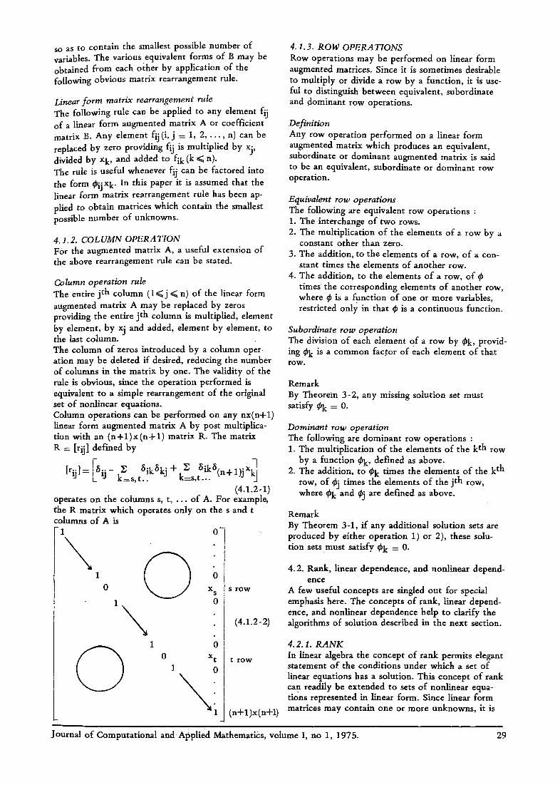
Column operation rule The entire j th column (1 <~j ~ n) of the linear form augmented matrix A may be replaced by zeros providing the entire j th column is multiplied, element by element, by xj and added, element by element, to the last column. The column of zeros introduced by a column oper- ation may be deleted if desired, reducing the number of columns in the matrix by one. The validity of the rule is obvious, since the operation performed is equivalent to a simple rearrangement of the original set of nonlinear equations. Column operations can be performed on any nx(n+l) linear form augmented matrix A by post multiplica- tion with an ( n + l ) x ( n + l ) matrix R. The matrix R = [rij ] defined by

[rij] = 18i. - E ~ikSkj + k~= s,~ik~(n+ 1)j x ~ LJ k = s , t . . . . . .

(4.1.2-1) operates on the columns s, t . . . . of A. For example, ehe R matrix which operates only on the s and t columns of A is

1

\ 1

0 C \

1

C) 0

0- I

0

X s

0 S rOW

(4.1.2-2)

0

Xt t r o w

OI

",iJ

4.1.3. ROW OPERATIONS Row operations may be performed on linear form augmented matrices. Since it is sometimes desirable to multiply or divide a row by a function, it is use- ful to distinguish between equivalent, subordinate and dominant row operations.

Definition Any row operation performed on a linear form augmented matrix which produces an equivalent, subordinate or dominant augmented matrix is said to be an equivalent, subordinate or dominant row operation.

Equivalent row operations The following are equivalent row operations : 1. The interchange of two rows. 2. The mukiplication of the elements of a row by a

constant other than zero. 3. The addition, to the elements of a row, of a con-

stant times the elements of another row. 4. The addition, to the elements of a row, of ~b

times the corresponding elements of another row, where ¢ is a function of one or more variables, restricted only in that ~b is a continuous function.

Subordinate row operation The division of each element of a row by q~k, provid- ing ~b k is a common factor of each element of that r o w .

Remark By Theorem 3-2, any missing solution set must satisfy ~k = 0.

Dominant row operation The following are dominant row operations : 1. The multiplication of the elements of the k th row

by a function ~b k, defined as above. 2. The addition, to ~k times the elements of the k th

row, of ~bj times the elements of the j th row, where ~b k and ~bj are defined as above.

Remark By Theorem 3-1, ff any additional solution sets are produced by either operation 1) or 2), these solu- tion sets must satisfy ~k = 0.

4.2. Rank, linear dependence, and nonlinear depend- ence

A few useful concepts are singled out for special emphasis here. The concepts of rank, linear depend- ence, and nonlinear dependence help to clarify the algorithms of solution described in the next section.

4.2.1. RANK In linear algebra the concept of rank permits elegant statement of the conditions under which a set of linear equations has a solution. This concept of rank can readily be extended to sets of nonlinear equa- tions represented in linear form. Since linear form matrices may contain one or more unknowns, it is

Journal of Computational andApplied Mathematics, volume I, no 1, 1975. 29

necessary to distinghuish between unconditional rank and conditional rank.

Definition The unconditional rank of a linear form coefficient or augmented matrix is the order o f the largest square array in that matrix (formed by deleting certain columns and rows) whose determinant does not vanish identically.

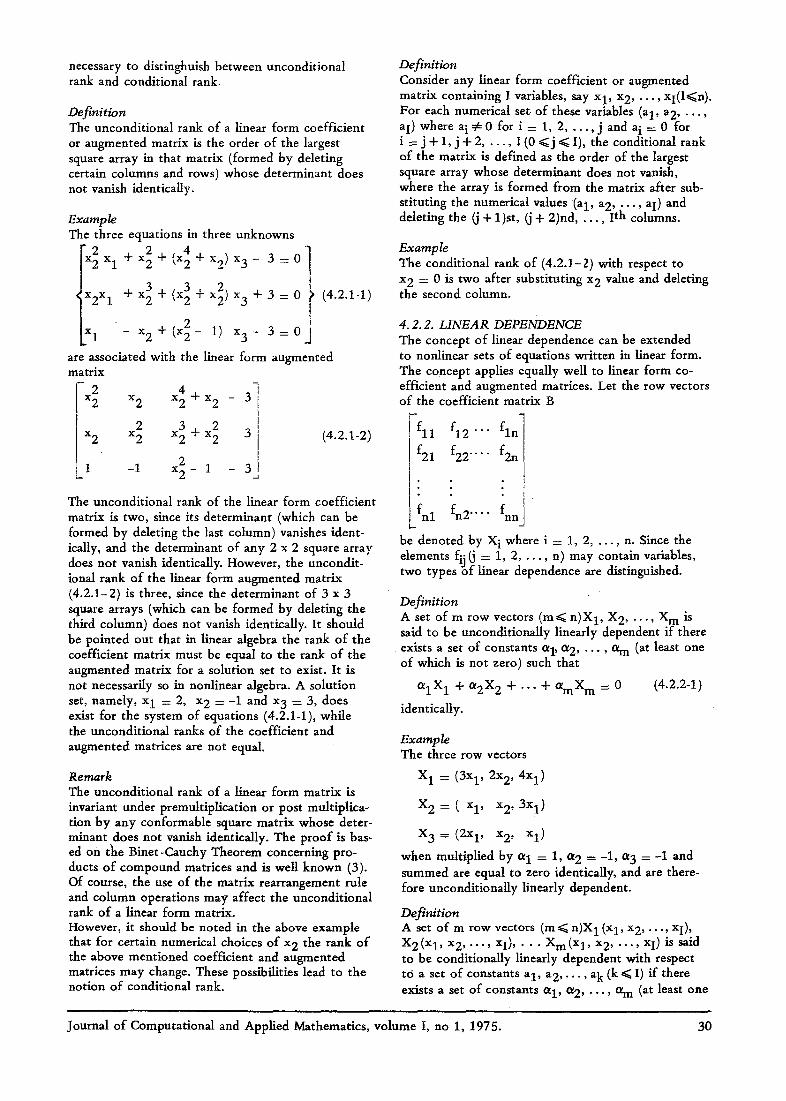
Example The three equations in three unknowns

r 2 2 4 ] !x 2 x 1 + x 2 + ( x 2 + x 2 ) x 3 - 3 = 0

! 3 2

x2x I + x ~ + ( x 2 + x 2 ) x 3 + 3 = 0 1 (4.2.1-1) t

2 ! x I - x 2 + ( x 2 - 1) x 3 - 3 = 0 J

are associated with the linear form augmented

x 2 + x 2 - 3

3 2 I x 2 x 2 + x 2 3 [

I o

1 -1 x ~ - 1 - 31 -.-I

matrix

x~ x 2

2 x 2 (4.2.1-2)

The unconditional rank of the linear form coefficient matrix is two, since its determinant (which can be formed by deleting the last column) vanishes ident- ically, and the determinant of any 2 x 2 square array does not vanish identically. However, the uncondit- ional rank of the linear form augmented matrix (4.2.1-2) is three, since the determinant of 3 x 3 square arrays (which can be formed by deleting the third column) does not vanish identically. It should be pointed out that in linear algebra the rank of the coefficient matrix must be equal to the rank of the augmented matrix for a solution set to exist. It is not necessarily so in nonlinear algebra. A solution set, namely, x 1 = 2 , x 2 = - 1 a n d x 3 = 3 , d o e s exist for the system of equations (4.2.1-1), while the unconditional ranks of the coefficient and augmented matrices are not equal.

Remark The unconditional rank of a linear form matrix is invariant under premultiplication or post multiplica- tion by any conformable square matrix whose deter- minant does not vanish identically. The proof is bas- ed on the Binet-Cauchy Theorem concerning pro- ducts o f compound matrices and is well known (3). Of course, the use of the matrix rearrangement rule and column operations may affect the unconditional rank of a linear form matrix. However, it should be noted in the above example that for certain numerical choices of x 2 the rank o f the above mentioned coefficient and augmented matrices may change. These possibilities lead to the notion of conditional rank.

Definition Consider any linear form coefficient or augmented matrix containing I variables, say Xl, x 2 . . . . . x i ( I ~ n ). For each numerical set of these variables (a 1, a 2, . . . , ai) wherea i ~ 0 f o r i = 1 , 2 . . . . . j a n d a i = 0 for i = j + 1, j + 2 . . . . . I (0 ~ j ~ I), the conditional rank of the matrix is defined as the order of the largest square array whose determinant does not vanish, where the array is formed from the matrix after sub- stituting the numerical values (al, a 2 . . . . . ai) and deleting the (j + 1)st, (j + 2)nd . . . . . Ith columns.

Example The conditional rank of (4.2.1-2) with respect to x 2 = 0 is two after substituting x 2 value and deleting the second column.

4.2. 2. LINEAR DEPENDENCE The concept o f linear dependence can be extended to nonlinear sets of equations written in linear form. The concept applies equally well to linear form co- efficient and augmented matrices. Let the row vectors of the coefficient matrix B

f l l f12 " '" f ln

f21 f22 . . . . f2n

f n 2 . . . .

be denoted by X i where i = 1, 2 . . . . , n. Since the elements fij {J = 1, 2 . . . . . n) may contain variables, two types o f linear dependence are distinguished.

Definition A set of m row vectors ( m E n)X 1, X 2 . . . . . X m is said to be unconditionally linearly dependent if there exists a set of constants 0l 1, 0t 2, . . . , ~cn (at least one of which is not zero) such that

a l X 1 + a2X 2 + . . . + ~mXm = 0 (4.2.2-1)

identically.

Example The three row vectors

X 1 = (3x 1, 2x 2, 4x 1)

X 2 = ( x 1, x 2 , 3 x 1)

X 3 = (2x 1, x 2, x 1)

when multiplied b y 41 = 1, 0~ 2 = -1, a 3 = -1 and summed are equal to zero identically, and are there- fore unconditionally linearly dependent.

Definition A set of m row vectors (m ~ n)X 1 (x 1, x 2 . . . . . xi), X2(Xl, x2, . . . , xi) , . . . Xm(Xl, x 2 . . . . . xi) is said to be conditionally linearly dependent with respect to a set of constants a l , a 2 . . . . . a k (k ~ I) ff there exists a set of constants Ol, ~2, " " , %n (at least one

Journal of Computational and Applied Mathematics, volume I, no 1, 1975. 30

of which is not zero) such that

C~lXl(al . . . . . a k, Xk+l . . . . . x I)

+ ~2X2(al . . . . . ak,Xk+ 1 . . . . . Xl) + . . .

+~VmXm(al . . . . . ak, X k + l , . . . , X l ) = 0

when the constants a 1, a 2 . . . . . a k have been sub- stituted for the variables x 1 . . . . . x k which appear in the row vectors.

Example Let the first two row vectors of the linear form augmented matrix (4.2.1-2) be denoted by X 1 (x2) and X2(x2). If x 2 = -1, there exist ~1 = 1, c~ 2 = l

such that

X1(_1 ) + X 2 ( - I ) = 0.

Therefore X 1 and X 2 are conditionally linearly de- pendent with respect to x 2 = -1. The following Theorem, based on the concept of linear dependence or conditional rank, is useful for testing the validity and character of a numerical solu- tion set. THEOREM 4-1 Let A and B be n x ( n + l ) and nxn linear form aug- mented and coefficient matrices associated with a set of n nonlinear equations with n unknowns. Let these matrices contain I variables xi( j = 1, 2 . . . . . I) where I <~ n. Let A c and Bc be theJcorresponding matrices after column operations on all j columns. A numerical set of values for xj, say 7j(j = 1, 2 . . . . ,I) (1) is not a part o f any solution set o f the original

nonlinear equations if and only if the conditional rank of A c :# the conditional rank of Be.

(2) is a part of a unique solution set of the original nonlinear equations ff and only if the conditional rank o f A c = the conditional rank of Bc = n - I.

(3) is a part of an ( n - I - r ) fold infinity of solutions of the original nonlinear equations if and only if the conditional rank of A c = the conditional rank o f B c = r, where r < n - I.

All of the conditional ranks referred to are of course with respect to the set of constants 7j.

Proof Substitution of 7; for x] in A c and B c yields matrices

3 with constant elements. These constant matrices Ac and B c have the dimensions n x ( n + l - I ) and nx(n-I). Thus the nonlinear equations have been reduced con- ditiona~y to a set o f n linear equations with n-I un- knowns. The Theorem now follows directly from classical linear algebra.

4.2. 3. NONLINEAR DEPENDENCE The concept of linear dependence presented in Sec- tion 4.2. 2 can be extended to nonlinear dependence.

Definition A set of m row vectors X 1, X2, . . . , X m is said to be nonlinearly dependent if there exists a set of con-

tinuous functions or constants 41, 42 . . . . . 4m (at least one of which contains at least one variable) such that

41X 1 + 4 2 X 2 + . . . + 4 m X m = 0

identically.

Example The three row vectors of the coefficient matrix (4.2.1-2) when multiplied by 41 = - 1 , 42 = 1,

43 = x 2 - x 2 and summed are equal to zero identic-

ally, and are therefore nonlinearly dependent.

THEOREM 4-2 The p row vectors of any pxn matrix are nonlinearly dependent if and only if the unconditional rank of the matrix is less than p. The p row vectors o f a pxn matrix are nonlinearly independent if and only if the unconditional rank of the matrix is p.

Proof The proof of this Theorem is quite lengthy and is therefore not given in this paper (for proof see Ref (6)).

4.3. Systematic elimination Systematic elimination is a formal linear elimination technique which can often be used to eliminate certain linear variables and to reduce the number of equations which must be solved simultaneously. The technique is useful whenever it is possible to select m equations which contain m variables in linear fashion only, from the original n equations in n vari- ables. After application of this technique, n-m equa- tions in n-m variables remain to be solved simultane- ously.

Algorithm The algorithm for performing systematic elimination is as follows. (1) The augmented linear form matrix A which re-

presents the set of n equations in n unknowns is written down.

(2) The linear form matrix rearrangement rule (Sec- tion 4.1.1) is used to minimize the number of variables which appear in A.

(3) Select R rows which contain n-R or fewer un- knowns so as to maximize R.

(4) Form a new Rx (n + l ) matrix A' from these R r O W S .

(5) Perform a column operation on A' for each vari- able contained in A', and delete the column of zeros created. I f x 2 appears in A' operate on and then delete the second column, etc. If the result- ing matrix contains more than R + I columns, continue column operation and subsequent dele- tion on arbitrarily selected columns until exactly R + I columns remain. Through step (5) strict equivalence has been maintained.

(6) Using the generalized Cramer's rule (see Theorem 4-3, below) solve for the R variables which cor- respond to the first R columns in terms of the

Journal of Computational and Applied Mathematics, volume I, no 1, 1975. 31

remaining n -R variables. This step often intro- duces additional and missing solution sets as shown in the statement following Theorem 4-3.

(7) Substitute the results from step (6) into the un- used n-R equations, thus eliminating R variables. The n-R equations obtained contain n-R vari- ables.

(8) These n-R equations, which must be solved simultaneously using some other technique, to- gether with the R equations from step (6), form a new set of equations which is dominant or subordinate to the original set of equations.

Cramer's rule may be generalized in nonlinear algebra. Theorem 4-3 shows that the use of Cramer's rule may introduce additional solution sets. The state- ment following the Theorem applies specifically to step (6) of the systematic elimination algorithm.

Definition If P is a square transformation matrix, the matrix obtained from P by replacing each element by its cofactor and then interchanging rows and columns is called the adjoint of P, denoted by Adj P. The following is considered to be the nonlinear generalization of Cramer's rule.

THEOREM 4-3 If (1) P is a transformatio'n matrix

(2) F is an equation vector then

PF : 0 ...C IPIF = 0 [IAdj PI=0]

Proof PF = 0 in expanded form is

.... PI<FFI l P21 P22 P2n IF2]

• :

Pnl Pn2 Pn

=0

Premultiplying by Adj P = [Pji] yields

I Pl l P21 . . . . Pnl

P12. P22. Pn2.

LPIn .P2n Pnn

Pl l P12 " " P l n

P21 P22 " " P 2 n

Pnl Pn2 "'" Pnn

PI

\ o IPI

I p l

-1:1"

F 2

Fn

1i2 li0 Premultiplication of PF = 0 by Adj P, according to Theorem 3-1, may introduce additional solution sets

r

=0~

=0

which, if they exist, must satisfy IAdj P I = 0. In order to use the generalized Cramer's rule to solve for the vector X of the equation BX + C = 0, two operations are required, premultiplication by Adj B followed by premultiplication with

IBI -i I (4.3-I)

IBI

By Theorem 3-1 or 4-3, premultiplication by Adj B is a dominant operation and any additional roots if introduced must satisfy [Adj BI = 0. By Theorem 3-2, premultiplication by (4.3-1) is a subordinate operation, and any missing solution sets must satisfy IB[ = 0.

Remark If no variables are cancelled after premultiplying by (4.3-1), there is no possibility of missing any solu- tion sets.

Example The three equations in three unknowns

xy 2 + y + yz = 0 ]

xy + y 2 z + 1 = 0 1 x + y 2 _ z - 2 = 0

(4.3-2)

are associated with the linear form augmented matrix

y2 1 y 0

y 0 y2 1 (4.3-3)

L 1 y -1 - 2 j

Operating on the second column yields

y , J Y y2 1 (4.3-4) 1 -1 y 2 - 2

Using the generalized Cramer's rule on, e. g., the first and third equations yields

i -Y Y I _y3 [ (2-y2) =1 + y

y2 y y2 + y 1 -1 (4.3-5)

uation

y2 - y

z = 1 (2 -y2) = y 4 _ 2 y 2 _ y y2 y y2 + y 1 - 1

Substituting into the second as yet unused ec yields the algebraic equation in y

(_y3 + y ) y + y 2 ( y 4 2 y 2 _ y ) + 1 = 0 (y2 + y) (y2 + y)

Journal of Computational and Applied Mathematics, volume I, no 1, 1975. 32

which may be factored into

y ( y + l ) ( y + l ) (y - l ) (y2-y-1 ) = 0. (4.3-6)

y ( y + l ) According to the statement and remark following Theorem 4-3, equations (4.3-5) and (4.3-6) are dominant to (4.3-2) and the following numerical values of y obtained from the numerator of (4.3-6) contain all of the solutions o f the original problem (4.3-2).

y = 0 y = - I y = + l y = 1.618

y = -0.618 (4.3-7)

if any additional solution sets are present in (4.3-7) they must satisfy [Adj B[ = 0 which in this example is

t

Thas the roots y = 0 and y = -1 may correspond to additional solution sets. These two values are now checked by means of Theorem 4- !. Substituting y = 0 into (4.3-4) yields

I: 0 01 0 1 (4.3-9)

L1 -1 -2J Since the conditional rank of the coefficient matrix of (4.3-9) is one, and the conditional rank of the augmented matrix is two, y = 0 is not a solution set of the original problem (4.3-2). Substituting y = -1 into (4.3-4) yields

-hi -1 -1 1 1 (4.3-10)

-1 -1

Since the conditional rank of the coefficient matrix of (4.3-10) equals the conditional rank of the aug- mented matrix of (4.3-10) which equals one, y =-1 is part of a one-fold infinity of solutions of the original problem (4.3-2). By inspection this solution set is

x - z - l = 0 y = - I (4.3-11)

which represents a straight line. The remaining roots of (4.3-7), y = 1, y = 1.618 and y = -0.618, when substituted into (4.3-5) yield the remaining solution sets

x = 0 y = l z = - i

x = 20.618 y = 1.618 z = 0 (4.3-12)

x = 1.618 y = - 0 . 6 1 8 z = 0

Thus the original problem (4.3-2) has four solution sets as expressed by (4.3-11) and (4.3-12).

4.4. Singular elimination Singular elimination is a flexible elimination tech- nique which in favorable cases is more powerful than systematic elimination. Occasionally singular elimina-

don can eliminate certain nonlinear variables. The technique is based on the notion of nonlinear depend- ence already described in Section 4.2.3. The principle of singular elimination is as follows. Consider the nx (n+ l ) linear form augmented matrix A associated with n nonlinear equations in n un- knowns. After any number n + l - m of column oper- ations (0< m <~ n+ l ) , the equivalent nxm matrix A c takes the form

f l l f12 " " " f lm-1

fkl f k 2 " ' " ff~n-1

f, f, f, nl n2" " " nm-1

f ~ -

l m

% [i 1

= k

[xo

f ~

l m

f ~

km

f ~

nm 1

(4.4-1)

where X i (i = 1, 2 . . . . . n) are the n row vectors fil' f ' . f ' i2 . . . . im-l" If there exists a set of functions or constants @i (i = I, 2 . . . . . m) as defined in Section 4.2.3, i. e.,

~1 X1 + @2X2 + • • + @mXm = 0,

then

X1 f ' ' lm

" C Xk [@k'=ol

iX!o -X1 f ' l m

• t Xk-1 f k - l m

f, , f, 0 @1 lm+@2f2m +" "+@m nm

X k + l f k + l

X n f ' nm

so that all solution sets of A c must satisfy

f, , . . . f ' = @1 lm + ~2 f2m + + @m nm 0

(4.4-2)

(4.4-3)

The validity of this statement is assured by Theorem 3-1, since the matrix on the right can be obtained from the matrix on the left by premultiplication with the transformation P matrix,

1 ~ . . ~ 1

@1 . . . . @k-1 @k @k+l . . . . em 0 . . . 0 J

t

I

(4.4-4) whose determinant is @k" Clearly is @k is a non-zero constant the matrix on

Journal o f Computational and Applied Mathematics, volume I, no 1, 1975. 33

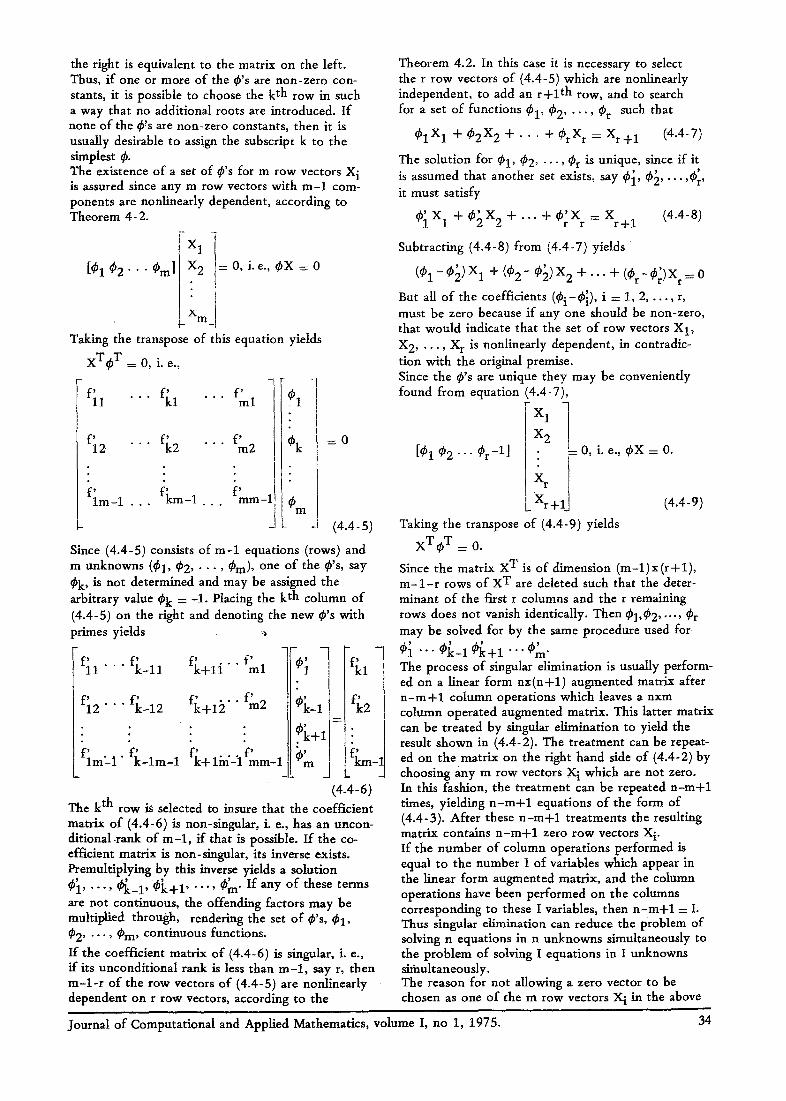
the right is equivalent to the matrix on the left. Thus, if one or more of the ¢'s are non-zero con- stants, it is possible to choose the k th row in such a way that no additional roots are introduced. If none of the ¢'s are non-zero constants, then it is usually desirable to assign the subscript k to the simplest ¢. The existence of a set of ~b's for m row vectors X i is assured since any m row vectors with m-1 com- ponents are nonlinearly dependent, according to Theorem 4-2.

[ ¢ 1 ¢ 2 " " ¢ m l 2 = 0 ' i ' e " ~ X = 0

l lm Taking the transpose of this equation yields

xT~b T = 0, i. e.,

f l l " " " fkl

fi2 fi 2 . , •

f lm-1 . . . fi m-1

f ' ~b 1 " " " ml

f, " ' " m2 k

b [ ram-1 Cm

" " " i

= 0

(4.4-5)

Since (4.4-5) consists of m-1 equations (rows) and m unknowns (¢1, ~b2, • "" , ~m), one of the O's, say ~bk, is not determined and may be assigned the arbitrary value ~k = -1. Placing the kth column of (4.4-5) on the right and denoting the new O's with primes yields :~

f l l " " f k - l l f k + l i " ' f ' • ml

, , f , . . f ' f12 " " " fk-12 k+12 " m2

f lm ' - I " f k - l m - 1 f ' f ' "k+ lln'-'l mm-I

- - - [ - - -

: l

: +111 = J

(4.4-6)

The k th row is selected to insure that the coefficient matrix of (4.4-6) is non-singular, i. e., has an uncon- ditional • rank of m - l , ff that is possible. If the co- efficient matrix is non-singular, its inverse exists. PremuMplying by this inverse yields a solution $1 . . . . . ¢k-1 ' ¢k+1 . . . . . Cm" If any o f these terms are not continuous, the offending factors may be multiplied through, rendering the set of cb's, ~b 1, ~b2 . . . . , Om, continuous functions.

If the coefficient matrix of (4.4-6) is singular, i. e., if its unconditional rank is less than m - l , say r, then m - l - r of the row vectors of (4.4-5) are nonlinearly dependent on r row vectors, according to the

Theorem 4.2. In this case it is necessary to select the r row vectors of (4.4-5) which are nonlinearly independent, to add an r + l TM row, and to search for a set of functions ¢1' ~b2 . . . . . Cr such that

¢1X1 + ¢2X2 + . . . + CrXr = X r + 1 (4.4-7)

The solution for ~1, ~2, " " , ~br is unique, since if it is assumed that another set exists, say ~1' ~b2 . . . . . Cr' it must satisfy

~1 X1 + ¢2 X2 + "'" + ¢~ Xr = X r + l (4.4-8)

Subtracting (4.4-8) from (4.4-7) yields

~ ' ~ X ( ~ b 1 - ¢ 2 ) X 1 + ( ¢ 2 ¢2) X 2 + " " + ( ¢ r - ¢ r ) r = 0

But all o f the coefficients (¢ i -¢ i ) ' i = 1, 2 . . . . . r, must be zero because if any one should be non-zero, that would indicate that the set o f row vectors X 1, X 2 . . . . . X r is nonlinearly dependent, in contradic- tion with the original premise. Since the ~b's are unique they may be conveniently found from equation (4.4-7),

X 1

X 2 [¢1 ¢ 2 " " ¢r -1] . = 0, i. e., ~bX = 0.

X r

L Xr+lJ (4.4-9)

Taking the transpose of (4.4-9) yields

X T c T = 0.

Since the matrix X T is of dimension (m- l ) x (r + 1), m - l - r rows of X T are deleted such that the deter- minant of the first r columns and the r remaining rows does not vanish identically. Then ~1,~b2 . . . . . Cr may be solved for by the same procedure used for

¢ i " '" ~bk-1 ¢ k + l "'" Cm" The process of singular elimination is usually perform- ed on a linear form n x (n + l ) augmented matrix after n - m + l column operations which leaves a nxm column operated augmented matrix. This latter matrix can be treated by singular elimination to yield the result shown in (4.4-2). The treatment can be repeat- ed on the matrix on the right hand side of (4.4-2) by choosing any m row vectors X i which are not zero. In this fashion, the treatment can be repeated n-m+1 times, yielding n - m + 1 equations of the form of (4.4-3). After these n - m + l treatments the resulting matrix contains n - m + 1 zero row vectors X i. If the number of column operations performed is equal to the number I of variables which appear in the linear form augmented matrix, and the column operations have been performed on the columns corresponding to these I variables, then n - m + l = I. Thus singular elimination can reduce the problem of solving n equations in n unknowns simultaneously to the problem of solving I equations in I unknowns simultaneously. The reason for not allowing a zero vector to be chosen as one of the m row vectors X i in the above

Journal of Computational and Applied Mathematics, volume I, no 1, 1975. 34

procedure is that the unconditional rank of the matrix formed from these m row vectors is often m-1. In this case, ff the kth row vector is zero the only set of O's which exist, namely 01 . . . . . Ok-1 = Ok+l ..... Om = 0 and Ok = any non-zero function or constant, is not useful for further reduc- tion by singular elimination.

Example The same problem solved by systematic elimination in Section 4.3 is now treated by singular elimination.

xy 2 + y + y z = 0 " 1

xy + y 2 z + I ~ f (4.3-2) x + y 2 - z - 2 =

The linear form augmented matrix corresponding to these equations is

y2 1 y 0

y 0 y2 (4.3-3)

i y -i

Operating on the second column yields y2 y y ]

Y y2 1 J (4.3-4) 1 -1 y2_2

A set of 0's for carrying out the singular elimination is defined by

y2 Y _t [¢i 02 ¢31 Y y2 = 0

1 -1

Before solving for the O's, it is convenient to re- arrange the above matrix equation to

1 -1 1 [03 02 01 ] y y2 = 0, y2 y

Taking the transpose and assuming 02 = - 1 yields the following matrix associated with the unknowns 03 and OI

_ y y2

Reducing this matrix by a process similar to Gauss- Jordan reduction yields

I 1 0

0 1

so that 01 = 1 02 = -1 03 = y_y2

Forming the transformation matrix of the form of (4.4-4) by letting k = 2 yields 0 ]

1 -1 y

0 0

Premultiplying (4.3-4) by (4.4-10) yields the equivalent matrix

[: y:l[ y2 y2 ~" 0

-I y2_~ i

(4.4-10)

~ (y+l)(y-Yl)(y2-y-11

-1 y2-2 J

so that all of the solution sets of the original prob- lem must satisfy

(y+l) (y-l) (y2-y-1) = 0.

This result is identical with the results obtained when using systematic elimination, as shown in Section 4.3.

4. 5. Triang,11ar elimination Triangular elimination is an alternate reduction tech- nique for treating linear form matrices. As with singular elimination this technique can also reduce n equations in n variables to I equations in I variables, where I is the number of variables contained in the linear form matrix. Triangular elimination is a repet- itive procedure mechanically similar to the Gauss reduction in linear algebra and may therefore be the best of the linear form reduction techniques for computer implementation.

Algorithm The algorithm for performing triangular elimination is as follows : (1) The augmented linear form matrix which re-

presents the set of n equations in n unknowns is written down.

(2) The linear form matrix rearrangement rule (Sec- tion 4.1.1) is used to minimize the number of variables which appear in the matrix.

(3) Perform any number of column operations (Sec- tion 4.1.2). It is usually advantageous to perform I column operations on the columns correspond- ing to the I variabhs which appear in the matrix.

(4) Rearrange the rows such that the 1, 1 element of the matrix becomes the simplest possible non- zero function, preferably a non-zero constant. Denote this column operated augmented matrix by A~ 1] .

. . . .

411J 1 41J . . . .

411 ,i 1 . . . .

n l . . . . t i m n x m

Journal of Computational and Applied Mathematics, volume I, no 1, 1975. 35

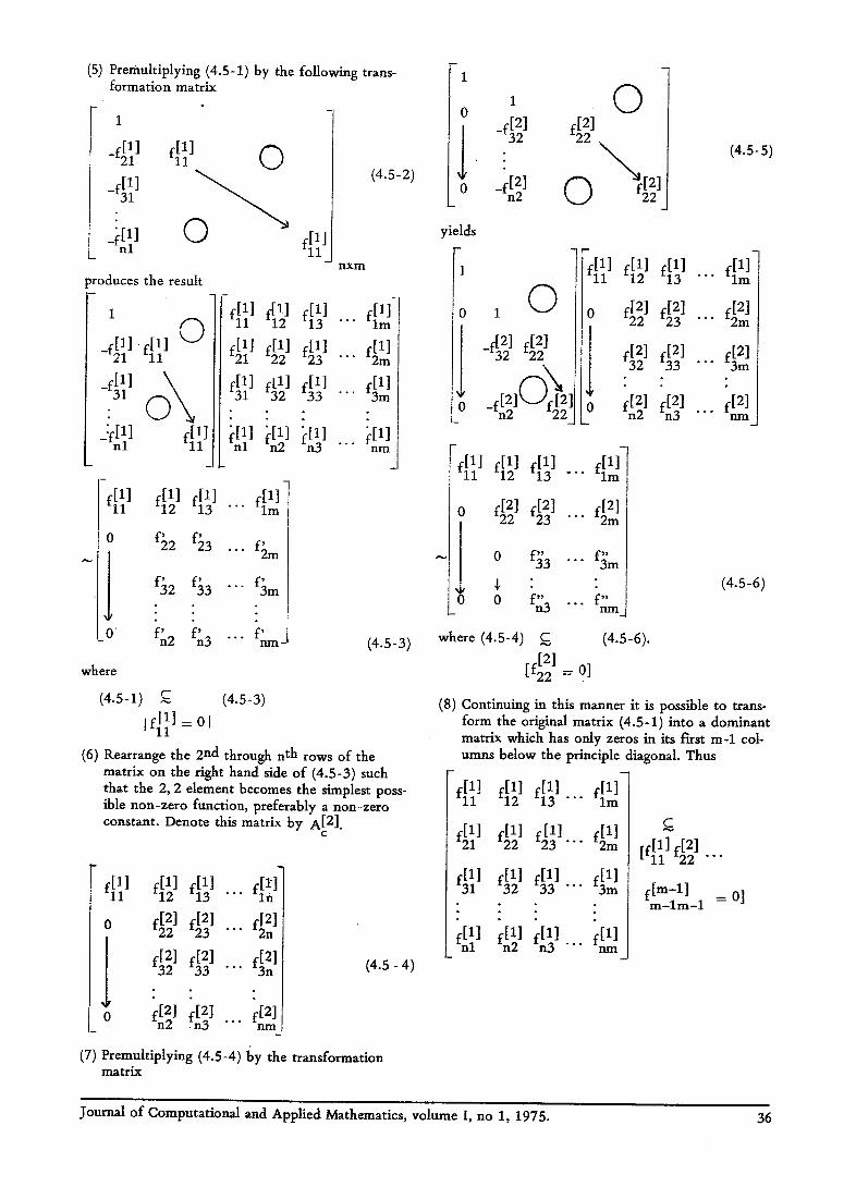
(5) Prernultiplying (4.5-1) by the following trans- formation matrix

1

-4 f -41] _L(~?

)roduces the result

1

4lj ,~] 0 _f[1131 O ~

_-'f [ 1] nl fill

~l] ] 0

fl] ] f[1] 21 f i l l 31

L[l]

d f[l] fi l l 22 23

fll]32 fi~ ]

n x m

(4.5-2)

,2t~

~[1] nm

12 13 "'"

o f;2 f;.3

2 3

0 f' f' - n2 n3

f , 2m

f, 3m

f ~

n l -n

where

(4.5-3)

(4.5-1) ,,,C (4.5-3)

lql]=0, (6) Rearrange the 2 nd through nth rows of the

matrix on the fight hand side of (4.5-3) such that the 2, 2 element becomes the simplest poss- ible non-zero function, preferably a non-zero constant. Denote this matrix by A[2].

C

0 f[2122 4 ~ ]

f[2] f[2] 32 33

o f f ~[3]

• .. ,i~]] • .. 4f"

f[2] "'" 3n

. . . f [ 2 ] n l T l

(4.5- 4)

(7) Premultiplying (4.5-4) by the transformation matrix

1 I 0

o _f[21 f[21 ~ 3 2 2 2 ~ f ~

0 _f[21 n2 O ]

(4.5-5)

yields

1

0 0 o 4f

-~3f4f Iti '3(f

f[21 23

,~2j

Cf f[21 3m

f[21 n l T l

i 4]] ,[~1 4~ 23 "'"

o 5 ' 3 f" "" 3 m

4 J" 0 0 f" f" n3 "'" nm~

where (4.5-4) C (4.5-6).

.[21 o] t22 =

(4.5-6)

(8) Continuing in this manner it is possible to trans- form the original matrix (4.5-1) into a dominant matrix which has only zeros in its first m-1 col- umns below the principle diagonal. Thus

W"

f i l l f[1] f [ l l f [ l ] 12 13 "'" lm

'"]~.~ 4]? ,~]l... 4~

31 32 "'"

fill fill ~ ] fill n l n 2 " '" n m

C

~,iI]f[2] 22 "'"

f [m- l l - Ol m- lm-1 -

Journal of Computational and Applied Mathematics, volume I, no 1, 1975. 36

~11 12 "'" lm-1

23 "" 2m-1

f[31 f[3t f[3] 3 3 - " " 3m-1 om

I

rim:l] . f[m-1 ] m-xm- i m - l m

C fire1 mm

" '4.

--I

L f[m] m m --I

If in step (3) I column operations are performed, then the solution sets of the matrix on the right hand side of (4.5-7) are found by solving the n - m + t = I equations containing t variables

£[m~ = 0 .rD_rD_

f[m] = 0 (4.5-8) m + l m

(4.5-7)

fim] = 0

and substituting back into the matrix on the right hand side of (4.5-7), providing none of the diagonal dements Ln the first m-1 columns of the matrix on the right hand side of (4.5-7) are zero. (9) Any solution set of (4.5-8) which makes one or

more of the diagonal elements of the matrix on ~che right hand side of (4.5-7) zero is tested by substituting it back into the original column

operated augmented matrix A[cl]. Such solution sets of (4.5-8) are accepted or rejected on the basis of rank according to Theorem 4-1.

Example The same problem solved by systematic elimination in Section 4.3 and singular elimination in Section 4.4 y2 y

t_ 1 -1 y2_ 2

is now treated by triangular elimination. First, the order of the rows is changed to place the third row first

y2_ 2- 1 -1

y y2

y2 Y Y A

(4.3-4)

(4.5-9)

Second, premultiplying by a transformation matrix

F I -y

0

i

0

0-[1 °IY 1 i y 2

-1

-1

y2

Y

y 2 - 2 1

yJ

I 1 1 -1 y2_1

y 2 + y l_(y2_2)y

y 2 + y y_y2 (y2_2) (4.5-10)

Thkd, premultiply by a constant transformation m a t r i x

0 0 1 -1 y2_1

l~ 1 0 y 2 + y l_(y2_2)y

-1 1_ y2+y y_y2(y2_2 )

"" 0 y2+y (4.5-11)

t0 0 Since it has been possible to maintain equivalence throughout these transformations, the solution sets of the original problem must satisfy

(y + 1) (y- 1 ) (y2-y- 1) = 0 (4.5-12)

i. e . ,

y = 1 y = -1 y = 1.618 y = -0.618

Substituting into the matrix on the right hand side of (4.5-11) yields the four solution sets expressed by (4.3-11) and (4.3-12).

y2-i

i-(y2-2)y

-(y+ l)(y-l)(y2-y-1)

9. BIBLIOGRAPHY I. Uspensky, J. V., "Theory of equations", First Edition,

McGraw-Hill Book Company, Inc., New York (1948).

2, Burnside, W. S., Panton, A. W., "Theory of equations", Third Edition, Hodges, Figgs, and Co., Dublin (1892).

3. Aitken, A. C., "Determinants and matrices", Ninth Edi- tion, Oliver and Boyd, Section 41, pp. 96-9? (1958).

4. Griffiths, L. W., "Introduction to the theory of equa- tions", Second Edition, John Wiley and Sons, New York, pp. 218-220 (1947).

5. Chrystal, G., "Algebra", Third Edition, Adam and Charles Black, London (1892).

6. Wu, C. L., "Nonlinear matrix algebra and engineering applications", Ph.D. Thesis, Case Institute of Technology (1964) .

Journal of Computational and Applied Mathematics, volume I, no 1, 1975. 37