NONLINEAR MODAL ANALYSIS AND SUPERPOSITION K. K. F. Wong 1 and J. L. Harris 2 ABSTRACT The linear modal analysis and superposition technique has been used extensively in earthquake engineering and seismic applications for decades, and it is extended herein to the nonlinear domain by representing the material nonlinearity using the force analogy method and computing the modal dynamics using the state space method. Combining these two methods with the modal analysis technique provides a significant advancement in developing a simplified, efficient, and comprehensive approach to performing nonlinear dynamic analysis. Numerical simulation is performed and the results are compared with Perform-3D commercial software to validate the proposed algorithm. Results show that the proposed algorithm possesses high accuracy and computational efficiency. Introduction Since the time when Newmark (1959) introduced the linear response history analysis for studying seismic effects on civil engineering structures, the development of current seismic design procedures relies heavily on this type of analysis technique because of its simplicity in the calculation procedure when the structural representation is transformed into the modal coordinates. Based on the analysis of a collection of single degree of freedom (SDOF) systems in each respective coordinate, the originally proposed response history analysis approach has been successfully extended to the popular response spectra approach that can give good representations of structural responses due to general seismic characteristics based on a variability of soil types and conditions. Once the maximum modal responses are determined in the response spectra approach, modal superposition is employed to determine the maximum structural responses. Although linear dynamic analysis based on linear response spectra approach is so popular, it has a shortcoming because all structures are designed with the anticipation that they will behave nonlinearly when a major earthquake occurs. Significant research works have been attempted to extend the linear dynamic analysis to the nonlinear domain (Liu 2003 and 2005, Au and Yan 2008), but presently nonlinear dynamic analysis techniques were employed in seismic design only in some special occasions mainly because the analysis itself is a time-consuming process. Current numerical algorithms require significant computation time to update the stiffness matrix to accommodate for nonlinearity in structures. In addition, many simulations need to be considered due to the uncertainties in earthquake ground motions. Therefore, the development of a nonlinear dynamic analysis algorithm that is both accurate and efficient remains as a challenge. 1 Research Structural Engineer, National Institute of Standards and Technology, Gaithersburg, MD 20899-8603 2 Research Structural Engineer, National Institute of Standards and Technology, Gaithersburg, MD 20899-8603 Proceedings of the 9th U.S. National and 10th Canadian Conference on Earthquake Engineering Compte Rendu de la 9ième Conférence Nationale Américaine et 10ième Conférence Canadienne de Génie Parasismique July 25-29, 2010, Toronto, Ontario, Canada • Paper No 363
Transcript
NONLINEAR MODAL ANALYSIS AND SUPERPOSITION
K. K. F. Wong1 and J. L. Harris2
ABSTRACT The linear modal analysis and superposition technique has been used extensively
in earthquake engineering and seismic applications for decades, and it is extended herein to the nonlinear domain by representing the material nonlinearity using the force analogy method and computing the modal dynamics using the state space method. Combining these two methods with the modal analysis technique provides a significant advancement in developing a simplified, efficient, and comprehensive approach to performing nonlinear dynamic analysis. Numerical simulation is performed and the results are compared with Perform-3D commercial software to validate the proposed algorithm. Results show that the proposed algorithm possesses high accuracy and computational efficiency.
Introduction Since the time when Newmark (1959) introduced the linear response history analysis for studying seismic effects on civil engineering structures, the development of current seismic design procedures relies heavily on this type of analysis technique because of its simplicity in the calculation procedure when the structural representation is transformed into the modal coordinates. Based on the analysis of a collection of single degree of freedom (SDOF) systems in each respective coordinate, the originally proposed response history analysis approach has been successfully extended to the popular response spectra approach that can give good representations of structural responses due to general seismic characteristics based on a variability of soil types and conditions. Once the maximum modal responses are determined in the response spectra approach, modal superposition is employed to determine the maximum structural responses. Although linear dynamic analysis based on linear response spectra approach is so popular, it has a shortcoming because all structures are designed with the anticipation that they will behave nonlinearly when a major earthquake occurs. Significant research works have been attempted to extend the linear dynamic analysis to the nonlinear domain (Liu 2003 and 2005, Au and Yan 2008), but presently nonlinear dynamic analysis techniques were employed in seismic design only in some special occasions mainly because the analysis itself is a time-consuming process. Current numerical algorithms require significant computation time to update the stiffness matrix to accommodate for nonlinearity in structures. In addition, many simulations need to be considered due to the uncertainties in earthquake ground motions. Therefore, the development of a nonlinear dynamic analysis algorithm that is both accurate and efficient remains as a challenge.
1Research Structural Engineer, National Institute of Standards and Technology, Gaithersburg, MD 20899-8603 2Research Structural Engineer, National Institute of Standards and Technology, Gaithersburg, MD 20899-8603
Proceedings of the 9th U.S. National and 10th Canadian Conference on Earthquake Engineering Compte Rendu de la 9ième Conférence Nationale Américaine et 10ième Conférence Canadienne de Génie Parasismique July 25-29, 2010, Toronto, Ontario, Canada • Paper No 363
In this research, linear dynamic analysis based on modal superposition is extended to analyzing structural responses in the nonlinear domain. This analysis technique can reduce the computation time without having to update the stiffness matrix. This nonlinear modal analysis (NMA) algorithm combines the force analogy method and the state space method in the modal coordinates. While the force analogy method is a simple nonlinear analysis tool based on initial stiffness and treats material nonlinearity as an equivalent force, the state space method a dynamic algorithm that can integrate explicitly to progress the effects of the equivalent force on structural responses to the next time step. Although some results focusing on fully nonlinear dynamic analysis have been published through the combination of these two methods (Yang et al. 2004, Zhang et al. 2007, Chao and Loh 2007, Wong and Johnson 2009), none of these works studied the nonlinear structural responses in the modal coordinate system. Therefore, it is the objective of this paper to demonstrate the accuracy and efficiency of the proposed NMA algorithm and present some applications of the analysis method based on reduced number of modes.
Force Analogy Method The detailed derivation of the force analogy method has been presented in Wong and Yang (1999). Let the total displacement )(tx at each degree of freedom (DOF) be represented as the summation of the elastic displacement )(tx′ and the inelastic displacement )(tx ′′ , i.e.,
)()()( ttt xxx ′′+′= (1) Similarly, let the total moment )(tm at the plastic hinge locations (PHLs) of a moment-resisting frame be separated into elastic moment )(tm′ and inelastic moment )(tm ′′ , i.e.,
)()()( ttt mmm ′′+′= (2) The displacements in Eq. 1 and the moments in Eq. 2 are related by the following equations:
)()( tt T xKm ′′=′ , )()()( 1 tt T ΘKKKKm ′′′′−′′−=′′ − (3) where )(tΘ ′′ is the plastic rotation at the PHLs, K is the global stiffness matrix, K ′ is the stiffness matrix that relates the plastic rotations at the PHLs and the forces at the DOFs, and K ′′ is the stiffness matrix that relates the plastic rotations with the corresponding moments at the PHLs. The relationship between plastic rotation )(tΘ ′′ and inelastic displacement )(tx ′′ is:
)()( 1 tt ΘKKx ′′′=′′ − (4) Substituting the two equations in Eq. 3 into Eq. 2 and making use of Eqs. 1 and 4, then rearranging the terms gives the governing equation of the force analogy method:
)()()( ttt T xKΘKm ′=′′′′+ (5)
Nonlinear Modal Analysis When the force analogy method is used, the elastic stiffness force is calculated by multiplying the initial stiffness matrix K with the elastic displacement )(tx′ . For an n-DOF system with plastic hinges at both ends of each member subjected to earthquake ground motion, the dynamic equilibrium equation of motion can therefore be written as
)()()()( tttt gMxKxCxM &&&&& −=′++ (6) where M is the nn× mass matrix, C is the nn× damping matrix, )(tx& is the 1×n velocity response at each DOF, )(tx&& is the 1×n acceleration response at each DOF, and )(tg&& is the 1×n ground acceleration vector corresponding to each DOF. Replacing the elastic displacement )(tx′ in Eq. 6 by the difference of total displacement )(tx and inelastic displacement )(tx ′′ gives
)()()()()( ttttt xKgMKxxCxM ′′+−=++ &&&&& (7) Let the modal displacement response )(tq
r be the 1×r vector of the form
[ ]Tr tqtqtqtt )()()()()( 21r
Lrrr
ΦqΦx == (8) where Φ is the rn× modal matrix – a collection of the first r mode shapes in column form:
[ ]rφφφΦ L21= (9) and r is the number of modes to be considered in the analysis, where nr ≤ . Differentiating the modal displacement )(tqr gives the modal velocity )(tq&
r , and differentiating it one more time gives the modal acceleration )(tq&&
r , i.e.,
)()( tt qΦx &r& = , )()( tt qΦx &&r&& = (10) Now substituting Eqs. 8 and 10 into Eq. 7 gives
Pre-multiplying Eq. 11 by TΦ and assuming that the damping matrix C exhibits proportional damping property, it follows from Eq. 11 that
)()()()()( ttttt TT xKΦgMΦqKqCqM ′′+−=++ &&rr&r
r&&r
r (12)
where MΦΦM T=
r, CΦΦC T=r
, and KΦΦK T=r
are the diagonal modal mass, modal damping, and modal stiffness matrices, respectively. This gives r modal equations of the form:
ritttqktqctqm Ti
Tiiiiiii ,...,1)()()()()( =′′+−=++ xKφgMφ &&
rr&rr&&rr (13) where imr , icr , and ik
r are the modal mass, damping, and stiffness, respectively, of the ith mode.
Note that these r modal equations in Eq. 13 are coupled through the last term of the equation.
State Space Method For all r modes given in Eq. 13, let the material nonlinearity term shown on the right side of the equation be treated as the equivalent modal force )(tpi
r , i.e.,
rittp Tii ,...,1)()( =′′= xKφr (14)
Then representing each modal equation in Eq. 13 in the state space form gives
iω and iζ are the natural frequency and damping ratio of the ith mode, respectively, and )(tair is
the modal ground acceleration of the ith mode that is computed by the formula:
rimtta iTii ,...,1)()( == r
&&r gMφ (17)
Solving for )(tg&& in Eq. 17 gives )()( tt aΦg
r&& = , where )(ta
r is the collection of all ground
accelerations in the modal coordinates and represented in the form:
[ ]Tr tatatat )()()()( 21r
Lrrr
=a (18) The term )(tg&& in Eq. 17, representing the ground acceleration at each DOF, can be expressed in terms of the three components of ground accelerations, )(tg X&& , )(tgY&& , and )(tgZ&& , as
[ ]TZYX tgtgtgtt )()()()()( &&&&&&
r&& haΦg == (19)
where h is the 3×n matrix that contains 0’s and 1’s depending on the direction of each DOF with respect to the corresponding the ground motion. Substituting Eq. 19 into Eq. 17 gives
[ ] ritgtgtgtgtgtgm
ta ZiZYiYXiXT
ZYXi
Ti
i ,...,1)()()()()()()( =Γ+Γ+Γ== &&&&&&&&&&&&rr Mhφ (20)
where iXΓ , iYΓ , and iZΓ are the modal participation factors for the ith mode in the x-, y-, and z-directions, respectively. The solution to the first order linear differential equation given in Eq. 15 is
[ ] ridssaspttt
tiiii
sti
tti
iii ,...,1)()()()(0
00
)( =++= ∫ −− rrrr HGeezez AAA (21) where 0t is the initial time. The state transition matrix tiAe of a SDOF system is
⎥⎥⎥⎥
⎦
⎤
⎢⎢⎢⎢
⎣
⎡
ωζ−
ζ−ωωζ−
ω−
ωζ−ω
ωζ−
ζ+ω= ωζ−
ttt
ttte
di
i
ididi
i
i
di
ii
di
i
idi
tt iii
sin1
cossin1
sin11sin
1cos
22
22Ae (22)
and diω is the damped natural frequency of the ith mode computed by the formula
21 iidi ζ−ω=ω (23) Define ttk =+1 , 0ttk = , and 0ttt −=Δ , it follows that Eq. 21 can be discretized and integrated as
riap ik
id
ik
id
ik
id
ik ,...,1)()()()()()()(
1 =++=+rrrr HGzFz (24)
where
tid
iΔ= AeF )( , titi
di Δ= Δ GeG A)( , ti
tid
i Δ= Δ HeH A)( (25)
)(ikzr , )(i
kpr , and )(ikar are the discretized forms of )(tizr , )(tpi
r , and )(tair , respectively, and the
superscript i in parenthesis denotes the calculation is based on the ith mode. Once the modal displacement and velocity responses embedded in )(i
kzr are obtained, the modal relative acceleration response can be calculated using Eq. 13 as
rimqkmqcampq ii
kiii
kii
kii
ki
k ,...,1)()()()()( =−−−= rrrr&rrrrr&&r (26) Finally, the absolute acceleration of the ith mode, )(
,ikaq&&r , can be calculated by summing the
relative acceleration in Eq. 26 with the modal ground acceleration defined in Eq. 17, i.e.,
riaqq ik
ik
ika ,...,1)()()(
, =+= r&&r&&r (27)
Numerical Simulation Consider the six-story moment-resisting steel frame as shown in Fig. 1. The mass of each and every floor is assumed to be equal to 200 000 kg. Rigid-ends are included in the modeling of the beams and columns. The stiffness matrix is computed based on the structural configuration shown, and eigenvalue analysis is then performed. The resulting natural periods are summarized in Table 1 and the mode shapes are tabulated in Table 2. Table 1 also shows the natural periods obtained from Perform-3D. A 3% natural damping in all 6 modes of vibration is assumed. Finally, the modal mass imr , damping icr , and stiffness ik
r are presented in Table 3.
Figure 1. Six-story moment-resisting steel frame.
W36x210x1
x2
x3
x4
x5
x6
W36x210 W36x210
W36x210 W36x210 W36x210
W36x210 W36x210 W36x210
W36x150 W36x150 W36x150
W36x135
W27x94
W36x135
W27x94
W36x135
W27x94
W14
x283
W14
x500
W14
x500
W14
x283
W14
x257
W14
x455
W14
x455
W14
x257
W14
x193
W14
x342
W14
x342
W14
x193
7.62 m
4.27
m
7.62 m 7.62 m
4.27
m4.
27 m
4.27
m4.
57 m
4.57
m
PHL#1 #2 #3 #4
#5
#6
#7
#8
#9
#10
#11 #13 #15#12 #14 #16
#17 #19 #21#18 #20 #22
#29 #31 #33#30 #32 #34
#23
#24
#25
#26
#27
#28
#35
#36
#37
#38
#39
#40
Table 1. Comparison of natural periods of vibration.
Mode Period (Perform) Period (NMA) Mode Period (Perform) Period (NMA) 1 0.836 s 0.834 s 4 0.117 s 0.116 s 2 0.303 s 0.302 s 5 0.086 s 0.086 s 3 0.170 s 0.169 s 6 0.067 s 0.066 s
From Eq. 24 and the computed modal parameters presented in Table 3, the recursive equation for the first mode of vibration using a time step size of 01.0=Δt s can be expressed as
)1()1(
)1(
)1(
)1(1
)1(1
009968.0000050.0
46.82009968.0000050.0
992661.0565867.0009968.0997167.0
kk
k
k
k
k apq
q
q
q rr
&r
r
&r
r
⎥⎦
⎤⎢⎣
⎡−−
+⎥⎦
⎤⎢⎣
⎡+
⎪⎭
⎪⎬⎫
⎪⎩
⎪⎨⎧⎥⎦
⎤⎢⎣
⎡−
=⎪⎭
⎪⎬⎫
⎪⎩
⎪⎨⎧
+
+ (28)
where k
Tkp ΘKφ ′′′= 1
)1(r and 11)1( ma k
Tk
r&&
r gMφ= . Similarly, the recursive equation for the second mode of vibration becomes
)2()2(
)2(
)2(
)2(1
)2(1
009866.0000050.0
26.14009866.0000050.0
966155.0278893.4009866.0978483.0
kk
k
k
k
k apq
q
q
q rr
&r
r
&r
r
⎥⎦
⎤⎢⎣
⎡−−
+⎥⎦
⎤⎢⎣
⎡+
⎪⎭
⎪⎬⎫
⎪⎩
⎪⎨⎧⎥⎦
⎤⎢⎣
⎡−
=⎪⎭
⎪⎬⎫
⎪⎩
⎪⎨⎧
+
+ (29)
where k
Tkp ΘKφ ′′′= 2
)2(r and 22)2( ma k
Tk
r&&
r gMφ= . Similar recursive equations can be written for other modes. Since the plastic rotation kΘ ′′ couples each and every mode of the response, the analysis must be performed with all r modes running simultaneously. Here, r can range from 1 to 6 with
6=n for this example, where 1=r means the response is calculated using only 1 mode, and 6=r means the response is calculated using all 6 modes. Plastic rotations are assumed to be concentrated at one point at the end of the beam and at the bottom of the columns only, giving a total of 40 PHLs as shown in Fig. 1. The moment capacity cm is calculated based on the plastic moment of the member:
Zm sc σ= (30)
where sσ is the yield stress of steel, or 248.2 MPa, and Z is the plastic section modulus of the members. All beams are subjected to a 21.89 kN/m uniformly distributed gravity loads. Moment versus plastic rotation relationship of all plastic hinges is assumed to exhibit elastic-plastic behavior, and the interaction effect between moment and axial force on the moment capacities of column members is neglected. The plastic hinges are assumed to be located at the rigid ends without any offset.
Figure 2. 1995 Kobe earthquake acceleration time history.
Figure 3. Comparison of displacement responses between NMA and Perform-3D.
-1
-0.5
0
0.5
1
0 5 10 15 20
Gro
und
Acce
lera
tion
(g)
Time (s)
-30
-20
-10
0
10
20
30
40
0 5 10 15 20
Roof
Dis
plac
emen
t (c
m)
Time (s)
Perform 3DModal Analysis
-30
-20
-10
0
10
20
30
0 5 10 15 20
6th
Fl. D
ispl
acem
ent
(cm
)
Time (s)
Perform 3DModal Analysis
-25-20-15-10
-505
10152025
0 5 10 15 20
5th
Fl D
ispl
acem
ent
(cm
)
Time (s)
Perform 3DModal Analysis
-20
-15
-10
-5
0
5
10
15
20
0 5 10 15 20
4th
Fl. D
ispl
acem
ent
(cm
)
Time (s)
Perform 3DModal Analysis
-20
-15
-10
-5
0
5
10
15
0 5 10 15 20
3rd
Fl. D
ispl
acem
ent
(cm
)
Time (s)
Perform 3DModal Analysis
-10-8-6-4-202468
0 5 10 15 20
2nd
Fl. D
ispl
acem
ent
(cm
)
Time (s)
Perform 3DModal Analysis
Subjected to the 1995 Kobe earthquake time history as shown in Fig. 2, Figs. 3 and 4 compare the global displacement and absolute acceleration responses, respectively, between NMA using all six modes (i.e., 6=r ) and Perform-3D results. As shown in the figures, the comparisons indicate that there is an excellent match between the two results, particularly in the upper stories, but misses some of the peaks for the lower stories. This demonstrates that NMA is an accurate procedure in capturing the global response of the structure.
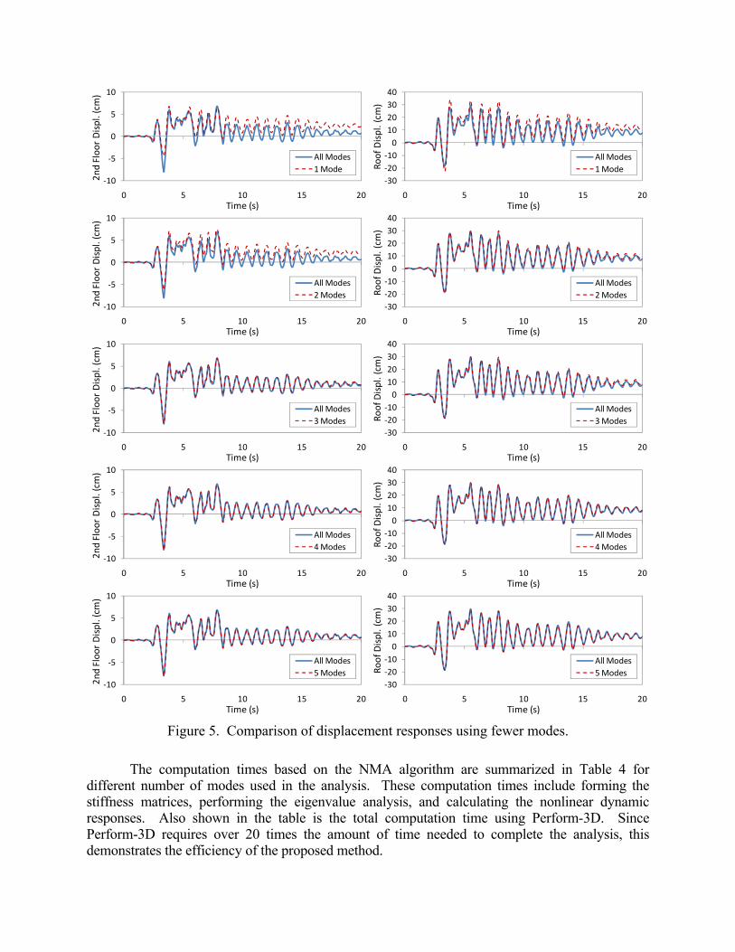
Figure 4. Comparison of absolute acceleration responses between NMA and Perform-3D. The NMA algorithm is now used to explore the possibility of reducing the number of modes in the analysis while maintaining the accuracy of results. Subjected to the 1995 Kobe earthquake time history, Fig. 5 compares the displacement of the second floor (left side of Fig. 5) and the roof (right side of Fig. 5) using reduced number of modes from 1=r to 5=r . It is observed that the response using only 1 mode (i.e., 1=r ) does not resemble the overall predicted response accurately, but the roof displacement response can obtain good accuracy when only 2 modes are used. Similarly, the second floor displacement response can obtain good accuracy when only 3 modes are used. This demonstrates the accuracy of the method even when using reduced number of modes, suggesting that the nonlinear response spectra approach can be exploited once a good understanding of the degree of coupling between modes is obtained.
-1.5
-1
-0.5
0
0.5
1
1.5
0 5 10 15 20
4th
Floo
r Ac
cele
ratio
n (g
)
Time (s)
Perform 3DModal Analysis
-1
-0.5
0
0.5
1
0 5 10 15 20
3rd
Floo
r Ac
cele
ratio
n (g
)
Time (s)
Perform 3DModal Analysis
-1-0.8-0.6-0.4-0.2
00.20.40.60.8
1
0 5 10 15 20
2nd
Floo
r Ac
cele
ratio
n (g
)
Time (s)
Perform 3DModal Analysis
-2
-1.5
-1
-0.5
0
0.5
1
1.5
0 5 10 15 20
Roof
Acc
eler
atio
n (g
)
Time (s)
Perform 3DModal Analysis
-1.5
-1
-0.5
0
0.5
1
1.5
0 5 10 15 20
6th
Floo
r Ac
cele
ratio
n (g
)
Time (s)
Perform 3DModal Analysis
-1.5
-1
-0.5
0
0.5
1
0 5 10 15 20
5th
Floo
r Acc
eler
atio
n (g
)
Time (s)
Perform 3DModal Analysis
Figure 5. Comparison of displacement responses using fewer modes. The computation times based on the NMA algorithm are summarized in Table 4 for different number of modes used in the analysis. These computation times include forming the stiffness matrices, performing the eigenvalue analysis, and calculating the nonlinear dynamic responses. Also shown in the table is the total computation time using Perform-3D. Since Perform-3D requires over 20 times the amount of time needed to complete the analysis, this demonstrates the efficiency of the proposed method.
-10
-5
0
5
10
0 5 10 15 20
2nd
Floo
r D
ispl
. (cm
)
Time (s)
All Modes1 Mode
-10
-5
0
5
10
0 5 10 15 20
2nd
Floo
r D
ispl
. (cm
)
Time (s)
All Modes2 Modes
-10
-5
0
5
10
0 5 10 15 20
2nd
Floo
r D
ispl
. (cm
)
Time (s)
All Modes3 Modes
-10
-5
0
5
10
0 5 10 15 20
2nd
Floo
r D
ispl
. (cm
)
Time (s)
All Modes4 Modes
-10
-5
0
5
10
0 5 10 15 20
2nd
Floo
r D
ispl
. (cm
)
Time (s)
All Modes5 Modes
-30-20-10
010203040
0 5 10 15 20
Roof
Dis
pl. (
cm)
Time (s)
All Modes5 Modes
-30-20-10
010203040
0 5 10 15 20
Roof
Dis
pl. (
cm)
Time (s)
All Modes4 Modes
-30-20-10
010203040
0 5 10 15 20
Roof
Dis
pl. (
cm)
Time (s)
All Modes3 Modes
-30-20-10
010203040
0 5 10 15 20
Roof
Dis
pl. (
cm)
Time (s)
All Modes2 Modes
-30-20-10
010203040
0 5 10 15 20
Roof
Dis
pl. (
cm)
Time (s)
All Modes1 Mode
Table 4. Computation time comparisons between NMA and Perform-3D.
A nonlinear dynamic analysis algorithm for computing the dynamic response of structures subjected to earthquake excitation based on modal superposition was presented. This algorithm combined the force analogy method and state space method while transforming the analysis into the modal coordinates. While modal coupling occurs because of the material nonlinearity in the structural model, this coupling is decomposed back into each mode using an equivalent modal force. Using the proposed algorithm, numerically simulated results were compared with those obtained from Perform-3D, and excellent correlation was obtained. These results demonstrate that the proposed algorithm is an excellent computational tool that contains high accuracy and efficiency. More importantly, it has the potential of expanding the scope of the nonlinear response spectra approach that may have great impact to seismic design.
Disclaimer Certain commercial software may be identified in this paper in order to specify the analytical procedure adequately. Such identification is not intended to imply recommendation or endorsement by the National Institute of Standards and Technology (NIST), nor is it intended to imply that the software identified are necessarily the best available for the purpose.
References Au, F.T.K. and Z.H. Yan, 2008. Dynamic analysis of frames with material and geometric nonlinearities
based on semi-rigid technique, International Journal of Structural Stability and Dynamics 8 (3), 415-438.
Chao, S.H. and C.H. Loh, 2007. Inelastic response analysis of reinforced concrete structures using modified force analogy method, Earthquake Engineering and Structural Dynamics 36 (12), 1659-1683.
Liu, J.L., 2003. Exact solution for dynamic response of multi-degree-of-freedom bilinear hysteretic systems, Journal of Engineering Mechanics ASCE 129 (11), 1342-1350.
Liu, J.L., 2005. Exact solution of nonlinear hysteretic responses using complex mode superposition method and its application to base-isolated structures, Journal of Engineering Mechanics ASCE 131 (3), 282-289.
Newmark, N.M., 1959. A method of computation for structural dynamics, Journal of Engineering Mechanics Division ASCE 85, 67-94.
Wong, K.K.F. and R. Yang, 1999. Inelastic dynamic response of structures using force analogy method, Journal of Engineering Mechanics ASCE 125 (10) 1190-1199.
Wong, K.K.F. and J. Johnson, 2009. Seismic energy dissipation of inelastic structures with multiple tuned mass dampers, Journal of Engineering Mechanic ASCE 135 (4), 265-275.
Yang, R., K.K.F. Wong, and T.C. Pan, 2004. Predictive inelastic state control of modern structures during earthquakes, Journal of Structural Control and Health Monitoring 11 (4), 291-309.
Zhang, X., K.K.F. Wong, and Y. Wang, 2007. Performance assessment of moment resisting frames during earthquakes based on force analogy method, Engineering Structures 29 (10), 2792-2802.