Nonlinear Models

and

Hierarchical Nonlinear Models

Start Simple

Progressively Add Complexity

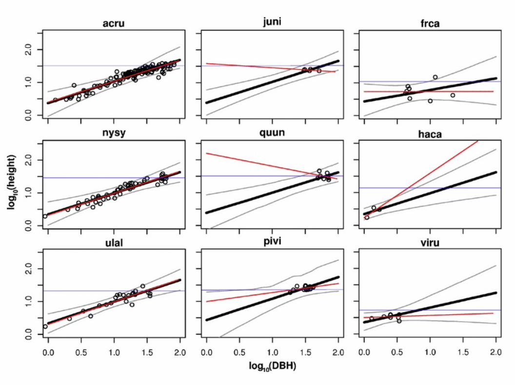
Tree Allometries

● Diameter vs Height with a hierarchical species effect

● Three response variables: Ht, crown depth, crown radius

● Crown radius as a latent variable● Heteroskedasticity in crown radius

Red Oak

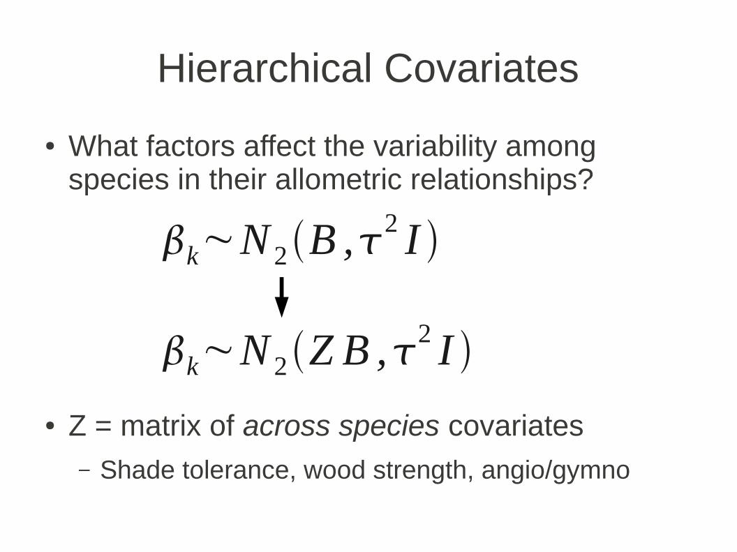
Hierarchical Covariates

● What factors affect the variability among species in their allometric relationships?

● Z = matrix of across species covariates– Shade tolerance, wood strength, angio/gymno

k~N 2B ,2 I

k~N 2Z B ,2 I

Tolerant

Intolerant

Weak

Strong

Prediction

● Hierarchical model structure would allow one to make predictions about an unobserved species

● Those predictions could be refined by knowing the hierarchical covariates

● Posterior for new species could be updated with a relatively small number of observations

● Structure could easily be extended to other forms of dependence (phylogenetic constraint, site covariates, etc.)

Summary

● Final Allometry model included– Multivariate Hierarchical linear model

– Hierarchical covariates

– Heteroskedasticity in radius

– Latent variables/Errors in variables on radius

– Borrowing strength / highly unbalanced dataInference on rare species

Assumption of linearity

● The final assumption of linear models that we'll address is that of linearity– Recall that linearity of models is wrt

parameters

● “Beastiary” of model from lecture 6(Bolker ch 3)

Assumption of linearity

● Consider any arbitrary function / process model y = g(x|θ

m)

– Choose a data model y ~ PDF( g(x|θ

m) , θ

d )

– If Bayesian, choose priors on θm

& θd

Fitting nonlinear models

● Rarely an analytical solution● Likelihood

– Numerical optimization– LRT or Bootstrap error estimates &

prediction● Bayes

– Metropolis-Hastings

Fitting nonlinear models

● Nothing you haven't seen / done before

● Nothing sacred about linear models

Things to watch for...

● Parameter identifiability

● Redundant parameters

Y=a

bc X

Y=1

b 'c ' X

Things to watch for...

● Odd correlations between parameters

Nonlinear Hierarchical Models

● Often takes more thought to decide which parameters you consider random and which are fixed

● Setting all parameters to random can often result in unidentifiablity

● Inclusion of covariates also challenging

Example: Coho salmon reproduction

● Beverton-Holt pop'n model with DD

● Consider– s = # of spawning Coho salmon

– r = # of recruits

● Reproduction varies by stream?– How can we incorporate random stream effect?

r t=st

1/st /rm

et

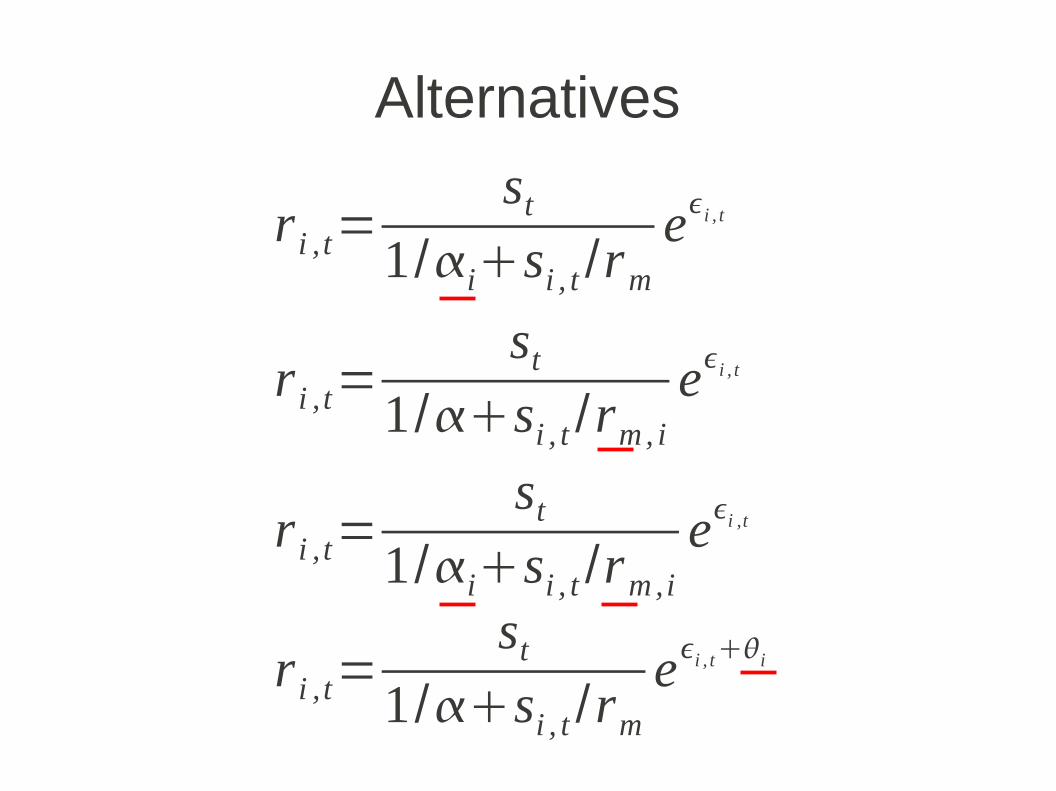
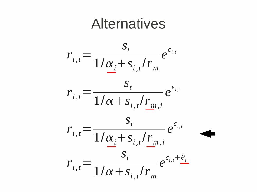
Alternatives

r i , t=st

1/isi , t /rm

ei , t

r i , t=st

1 /si , t /rm, i

ei , t

r i , t=st

1/isi , t /rm,i

ei ,t

r i , t=st

1/si , t /rm

ei , ti

Alternatives

r i , t=st

1/isi , t /rm

ei ,t

r i , t=st

1/si , t /rm,i

ei ,t

r i , t=st

1/isi , t /rm,i

ei , t

r i , t=st

1/si , t /rm

ei , ti

r i , t=st

1/isi , t /rm,i

ei , t Process model

i , t~N 0,2 Residual error

r i ,m~N r ,r2

i~N ,

2

Stream-level parameters

r~N r0,V r~N 0,V

Across stream parameters

,r~IG s1, s2 Across stream variance

Example: CO2 effect on tree seedling growth

● i – seedling

● j – plot

● t – year

● l – light

● y - growth

i , j , t=gi , j l j , t−lcl j , t

yi , j , t=i , j , tk ti , j , tyearmean residual

i , j , t~N 0,2

k t~N 0,k

gi , j~ln ,g

lc varies w/ CO2, Priors on α, v

g, v

k, σ2, θ, l

c

CO2 effect

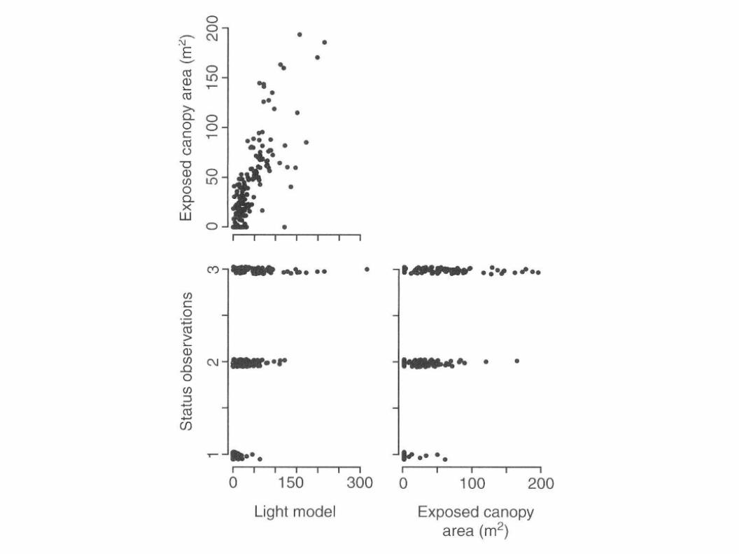
Canopy Light:Synthesizing multiple data sources

● Tree growth depends upon light (previous example, lab 7)

● Hard to measure how much light an ADULT tree receives

● Multiple sources of proxy data– Exposed Canopy Area

● aerial photography, Quickbird

– Canopy status ● suppressed, intermediate, dominant (ex 8.2.2)

– Light models● Allometries, stand map

Mechanistic Light Model• Estimate light levels based on a 3D ray-tracing light model

• Parameterized based on canopy photos, tree allometries

Linear models

Logistic

Multinomial

Exposed Canopy Area

● Error in relationship between “true” light λ and observations λe

● Probability of observing the tree in imagery increases with “true” light availability

p ie={ 1−pi i

e=0

pi N ln ie∣ln i ,e i

e0}

logit pi=c0c1i

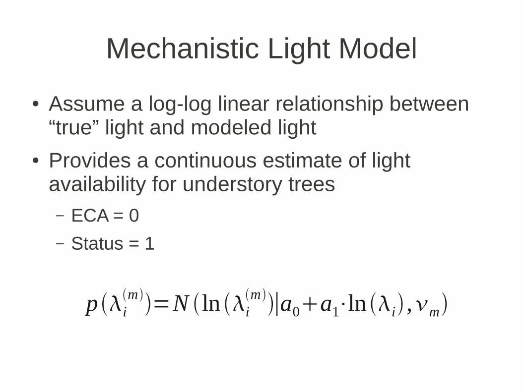
Mechanistic Light Model

● Assume a log-log linear relationship between “true” light and modeled light

● Provides a continuous estimate of light availability for understory trees– ECA = 0

– Status = 1

p im=N ln i

m∣a0a1⋅ln i ,m

Model Fitting

● Model fit all at once● Find the conditional probabilities for each

parameter (i.e. those expressions that contain that parameter)– Always at least 2 – likelihood and prior

– Can be multiple likelihoods

● MCMC iteratively updates each parameter conditioned on the current value of all others