NONLINEAR MULTIAXIAL MODELING OF GRAPHITIC … · model. The JNM model is necessary for materials...

AFML-TR-76*215

0 /

NONLINEAR MULTIAXIAL MODELING OF GRAPHITIC ANCARBON-CARBON MATERIALS

R01ERT M. JONESCIVI• & MECHANICAL ENGINEERING DEPARTMENTSCHOOL OF ENGINEERING AND APPLIED SCIENCESOUTHERN METHODIST UNIVERSITY-DALLAS, TEXAS 75275

DECEMBER 1976.

FINAL REPORT MARCH 1975 - JUNE 1976

Approved for public release; distribution unlimited

- AIR FORCE MATERIALS LABORATORY: i-- AIR FORCE WRIGHT AERONAUTICAL LABORATORIES- ;i AIR FORCE SYSTEMS COMMAND

WRIGHT-PATTERSON AIR FORCE BASE, OHIO 45433

NOTICE

When Government drawings, specifications, or other data are usedfor any purpose other than in connection with a definitely relatedGovernment procurement operation, the United States Government therebyincurs no responsibility nor any obligation whatsoever; and the fact thatthe Government may have formulated, furnished, or in any'way supplied thesaid drawings, specifications, or other data, is not to be regardedby implication or otherwise as in any manner licensing the holder or anyother person or corporation, or conveying any rights or permission tomanufacture, use, or sell any patented invention that may in any way berelated thereto. f

This technical report has been reviewed and is approved for publica-tion.

Clarence A. PrattProject MonitorSpace and Missiles BranchSystems Support DivisionAF Materials Laboratory

FOR THE DIRECTOR , .,.

* 1

4 A /.oo,.

Albert Olevitch, ChiefNon-Metals Materials BranchSystems Support DivisionAF Materials Laboratory

Copies of this report should not be returned unless return isrequired by security considerations, contractural obligations, ornotice on a specific document.

Best Avail- .

UNCLASSIFIEDSECURITY C•J4SIFICATION OF THIS PAGE (When Data Entered)(C•flREPORT DOCUMENTATION PAGE" EDISRCINSREAD INSTRUCTIONS

BEFORE COMPLETING FORM2. GOVT ACCESSION NO. 3. RECIPIENT'S CATALOG NUMBER

AFMIQtrR-76-?15___ _____________

4. TITLE (ard Subtitle) ,TYPE.OF REPORT-&.._ P Q2_COVERED /I•£NAL TECHNICAL---MT

NýONLINEAR IMULTIAXIAL MJODELING OF FNA TECHNICALMAI ]175---.J UNII 176•GRAPHITIC AND CARBON-CARBON MATERIALSI

noneAUTHOR(s) .J. CONTRACT OR GRANT NUMBER(s)

R T NkF33615-75-C-5212SROBERT ,.. . .

9. PERFORMING ORGANIZATION NAME AND ADDRESS 10. PROGRAM ELEMENT, PROJECT, TASKAREA 8 WORK UNIT NUMBERS

CIVIL AND MECHANICAL ENGINEERING DEPARTMENTSCHOOL OF ENGINEERING AND APPLIED SCIENCESOUTHERN METHODIST UNIVERSITY DALLAS, TX 75275 .

11. CONTROLLING OFFICE NAME AND ADDRESS 12. REPOR DATE --

AIR FORCE MATERIALS LABORATORY/MXS J 1976- c. 71WRIGHT-PATTERSON AFB, OHIO 45433 13. NUABE'-QF PAGE ...

_19, 197-14. MONITORING AGENCY NAME & ADDRESS(II different from Controlling Office) iTs. -SECUJITY'CLASS. (of thi]R report)

UNCLASSIFIED15a. DECLASSI FICATION/DOWNGRADING

SCHEDULE

16. DISTRIBUTION STATEMENT (of this Report)

Approved for Public Release; Distribution Unlimited D C3

17. DISTRIBUTION STATEMENT 'of the abstract entered in Block 20, If different from Report)

18. SUPPLEMENTARY NOTES . 0*

19, KEY WORDS (Continue on reverse Aide If necessary and identify hy block number)

Graphite, Carbon-Carbon, Composite Materials, Orthotropy, Anisotropy,Stress Analysis, Material Modeling

20 ABSTPLACT (Continue •on frverne xInei If ner.esarv atni IdentIfy byv hbnk number)/''The nonlinear material model due to Jones and Nelson is extended to

temperature-dependent material behavior and applied to the analysis of theSouthern Research Institute Thermal Stress Disk Test. The predicted diametraldeformations of the annular disk are within three percent of the measureddeformations at three times in a specific test. The Jones-Nelson model isexteinded to treatment of materials with first nonlinear then linear stress-strain behavior in what is called the Jones-Nelson-Morgan nonlinear materialmodel. The JNM model is necessary for materials with strona nonlinearities a_

DD ~ 7 2 A 1473 FOI? j oil I NOV 1,t 11, O n~no r.r ~UNCLASSIFI EDBestAvai a CopyN t I'Air 110-, r.ne P

-TBest Available COPY

UNCLASSIFIEDSFCURITY CLASSIFICATION OF THIS PAGE(I•hon DI. En•t•i.d)

BLOCK 20. ABSTRACT, continuedSis demonstrated for ATJ-S graphite in a reentry vehicle nosetip stress analy-

sis. The JNM model is also speculated to be useful for carbon-carbon materialbecause all pertinent numbers and types of nonlinearities can be treated. Alinear elastic multimodulus analysis is used to demonstrate that the ASTMFlexure Test does not lead to useful results for carbon-carbon and other multimodulus materials. Necessary future modeling work for carbon-carbon is out-lined.

?,

:1'

-- UNCLASSIFIED'. SECUR~ITY CLASSI•'iCATION OF THIII I'AE(WNmn I)mt. PtliledI

K.I

FOREWORD

This final report is submitted by the Civil and Mechanical Engi-neering Department, School of Engineering and Applied Science, SouthernMethodist University, Dallas, Texas 75275 under USAF Contract F33615-

75-C-5212. The work, an extension of the nonlinear deformation mate-rial model for graphitic reentry vehicle nosetip materials, was performedfor the Air Force Materials Laboratory, Wright-Patterson AFB, Ohio 45433.

The AFML/MXS project monitors in order of service were Captain CharlesL. Budde, Lt. Terry Hinnerichs, Captain Perry Cockerham, and Mr. Clarence

A. Pratt.Dr. Robert M. Jones was the Principal Investigator. The assistance

of Mr. Harold S. Morgan in developing and discussing the extended stress-

strain curve approach and the JNMDATA computer program is gratefullyacknowledged. The extensive cooperation of Mr. H. Stuart Starrett, Head,Analytical Section, Mechanical Engineering Division, Southern ResearchInstitute, Birmingham, Alabama 35205 in interpreting various experimental

results is sincerely appreciated.

,II

I•,

• . ,• . ,,....q~m b•, ,., •• •.. ... • .. • •, • ,, ,, .,'.• ,. • N .. . .. . 1

TABLE OF CONTENTS

LIST OF FIGURES ..................................................... viii

LIST OF TABLES ...................................................... xiii

1. INTRODUCTION ......................................1

1.1 BIAXIAL SOFTENING .......................................... I

1.2 DIFFERENT MODULI IN TENSION AND COMPRESSION ................ 4

1.4 CHARACTERISTICS OF CARBON-CARBON ..................... 121.4 CHARACTERISTICS OF CA B NCRAPHIT . ......... .................. 12

1.5 STATEMENT OF THE PROBLEM ............................ 151.6 STATEMENT OF RESEARCH ........................ ...... 16

1.6.1 PHASE G - GRAPHITE ........................... 16

1.6.2 PHASE C - CARBON-CARBON ...................... ...... 19

1.7 SCOPE OF REPORT ..................................... ...... 21

2. JONES-NELSON-MORGAN NONLINEAR MATERIAL MODEL ................ 23

2.1 INTRODUCTION ............................................... 23

2.2 JONES-NELSON NONLINEAR MATERIAL MODEL ...................... 232.2.1 BASIC APPROACH ...................................... 24

2.2.2 IMPLEMENTATION OF THE MATERIAL MODEL ................ 29

2.2.3 TEMPERATURE INTERPOLATION OF

DEFORMATION BEHAVIOR ................................ 43

2.2.3.1 Parameter Interpolation .................... 462.2.3.2 Property Interpolation ..................... 48

2.2.3.3 Stress-Strain Curve Interpolation .......... 50

2.2.3.4 Suninary .................................... 51

2.3 EXTRAPOLATION PROCEDURES FOR MATERIAL MODELS ............... 532.3.1 INTRODUCTION ........................................ 53

2.3.2 EXTENDED MECHANICAL PROPERTY VERSUS

STRAIN ENERGY CURVE APPROACH ........................ 55

2.3.3 EXTENDED STRESS-STRAIN CURVE APPROACH ............... 592.3.3.1 Linear Stress-Strain Curve Extensions

with Zero Slope ............................ 59

2.3.3.2 Linear Stress-Strain Curve Extensions

with Nonzero Slope ......................... 66

v

* p* 4,. ~ .- .I,

TABLE OF CONTENTS, continued

2.4 THE JNMDATA COMPUTER PROGRAM .................. ............ 70

3. MODELING OF GRAPHITIC MATERIALS ................................. 78

3.1 THERMAL STRESS DISK TEST CORRELATION ....................... 78

3.1.1 INTRODUCTION ........................................ 78

3.1.2 MEASUREMENTS OF TEMPERATURES AND DEFORMATIONS ....... 82

3.1.2.2 Overall Test Setup ......................... 823.1.2.2 Inner Diameter Temperature Measurement ..... 833.1.2.3 Outer Diameter Temperature Measurement ..... 84

3.1.2.4 Diametral Deformation Measurements ......... 85

3.1.2.5 Sunma y .................................... 85

3.1.3 PREDICTED Df5'.RMATIONS, STRESSES, AND STRAINS ....... 86

3.1.3.1 Jones-Nelson Nonlinear Material Model ...... 86

3.1.3.2 ATJ-S Graphite Mechanical Properties ....... 87

3.1.3.3 Inner Diameter Change Predictions .......... 92

3.1.3.4 Stress and Strain Predictions .............. 98

3.1.4 SUMMARY ............................................ 103

3.2 50 MW NOSETIP STRESS ANALYSIS ............................. 103

3.2.1 INTRODUCTION ....................................... 103

3.2.2 JONES-NELSON-MORGAN NONLINEAR MATERIAL MODEL

PREDICTIONS ........................................ 104

3.2,2.1 ATJ-S Graphite Mechanical Properties ...... 1043.2.2.2 Elastic Stress and Strain Predictions ..... 113

3.2.2.3 Nonlinear Stress and Strain Predictions...117

3.2.3 COMPARISON OF JONES-NELSON-MORGAN AND

DOASIS STRESS AND STRAIN PREDICTIONS ............... 122

3.2.4 SUMMARY OF 50 MW NOSETIP STRESS ANALYSIS ........... 127

3.3 SUMMARY OF GRAPHITIC MATERIAL MODELING .................... 129

4. MODELING OF CARBON-CARBON MATERIALS ............................ 131

4.1 INTRODUCTION .............................................. 131

4.2 CHARACTERISTICS OF CARBON-CARBON .......................... 131

4.3 APPARENT FLEXURAL MODULUS AND FLEXURAL STRENGTH

OF MULTIMODULUS MATERIALS ................................. 146

4.3.1 INTRODUCTION. ................................146

vi

K

4.3.2 APPARENT FLEXURAL MODULUS .......................... 150

4.3.3 APPARENT FLEXURAL STRENGTH ......................... 157

4.3.4 SUMMARY ............................................ 164

4.4 FUTURE MODELING WORK ...................................... 165

5. CONCLUDING REMARKS ............................................. 168

APPENDIX DETERMINATION OF THE POINT OF ZERO SLOPE ON

AN IMPLIED STRESS-STRAIN CURVE BY INTERVAL HALVING ....... 169

REFERENCES ......................................................... 173

vii

LIST OF FIGURES

1-1 BIAXIAL SOFTENING OF GRAPHITE ................................. 2

1-2 HOLLOW GRAPHITE SPECIMEN ...................................... 3

1-3 BIAXIAL STRAIN RESPONSE OF A HOLLOW

ATJ-.S GRAPHITE SPECIMEN AT ROOM TEMPERATURE

(70°F) AND 3550 psi PRINCIPAL STRESS .......................... 3

1-4 STRESS-STRAIN CURVE FOR A MATERIAL WITH

DIFFERENT MODULI IN TENSION AND COMPRESSION ................... 5

1-5 COMPARISON OF BILINEAR MODEL WITH ACTUAL BEHAVIOR ............. 7

1-6 BIAXIAL RESPONSE OF A HOLLOW ATJ-S GRAPHITE SPECIMEN

AT ROOM TEMPERATURE (70°F) AND 3550 psi PRINCIPAL STRESS ...... 9

1-7 BIAXIAL RESPONSE OF A HOLLOW ATJ-S GRAPHITE SPECIMEN

AT 200 0 'F AND 3550 psi PRINCIPAL STRESS ....................... 10

1-8 GRAPHITE BEHAVIOR ............................................. 11

1-9 CARBON-CARBON BEHAVIOR ........................................ 13

1-10 CARBON-CARBON PLUG NOSETIP .................................... 14

1-11 WEDGE-SHAPED DISK SPECIMEN .................................... 17

2-1 REPRESENTATION OF STRESS-STRAIN RELATIONS

FOR DIRECT MODULI AND POISSON'S RATIOS ........................ 27

2-2 ITERATION PROCEDURE FOR NONLINEAR MULTIMODULUS MATERIALS ...... 28

2-3 NONLINEAR SHEAR STRESS - SHEAR STRAIN CURVE ................... 30

2-4 REPRESENTATIVE MECHANICAL PROPERTY VERSUS U CURVE ............. 31

2-5 REPRESENTATIVE MECHANICAL PROPERTY VERSUS U BEHAVIOR

AND POSSIBLE APPROXIMATIONS ................................... 34

2-6 DATA POINTS WHICH LEAD TO PITFALLS IN CALCULATING B AND C.....38

2-7 MECHANICAL PROPERTY VERSUS IJ BEHAVIORS WHICH

"CAUSE DIFFICULTIES IN DETERMINING B AND C .................. 41

2-8 UNIAXIAL STRESS-STRAIN BEHAVIOR AND CORRESPONDING

MATERIAL PROPERTY VERSUS U BEHAVIOR ........................... 43

viii

:,• • .••.•W, b•, • • ,,,, ,.. -,.. .. ..... ... . :*• ' • • •..,,..... •.~ao,. ,- ... . ,• ,

LIST__OF FIGURES, continued

2.-9 ATJ-S GRAPHITE STRESS-STRAIN CURVES FOR 70°F AND 2000OF ....... 45

2-10 ATJ-S GRAPHITE MECHANICAL. PROPERTY (E ErVERSUS STRAIN ENERGY FOR 70°F AND 2000°F ...................... 45

2-11 STRESS-STRAIN CURVE AT 1403°F FROM PARAMETER INTERPOLATION .... 47

2-12 MECHANICAL PROPERTY VERSUS ENERGY CURVE AT 1403°FFROM PARAMETER INTERPOLATION .................................. 47

2-13 STRESS-STRAIN CURVE AT 1403°F FROM PROPERTY INTERPOLATION.....49

2-14 MECHANICAL PROPERTY VERSUS ENERGY CURVE AT 1403°F

FROM PROPERTY INTERPOLATION ................................... 49

2-15 NORMAL STRESS - NORMAL STRAIN BEHAVIOR

OF AN ORTHOTROPIC MATERIAL .................................... 54

2-16 ACTUAL AND EXTRAPOLATED MECHANICAL PROPERTY

VERSUS U BEHAVIOR ....................................... 55

2-17 EXTENDED IMPLIED STRESS-STRAIN CURVES

FORA=1, B .5,U0 = 1.................................... 57

2-18 REPRESENTATIVE IMPLIED STRESS-STRAIN BEHAVIOR

CORRESPONDING TO JONES-NELSON EQUATION ........................ 58

2-19 LINEAR STRESS-STRAIN CURVE EXTRAPOLATION WITH ZERO SLOPE

BY ARBITRARY EXTENSION OF STRESS-STRAIN DATA .................. 60

2-20 LINEAR STRESS-STRAIN CURVE EXTRAPOLATION WITH ZERO SLOPE

WITH BEST FIT EXTENSION OF STRESS-STRAIN DATA ................. 64

2-21 LINEAR STRESS-STRAIN CURVE EXTRAPOLATION WITH NONZERO SLOPE

WITH BEST FIT OF STRESS-STRAIN DATA ........................... 67


EQUAL TO SLOPE AT LAST DATA POINT ............ v ............... 69

2-23 PLOTS OF ACTUAL STRESS-STRAIN DATA AND

CORRESPONDING MECHANICAL PROPERTY VERSUS ENERGY DATA .......... 71Ii'I

2-24 JONES-NELSON NONLINEAR MATERIAL MODEL

FOR DATA OF FIGURE 2-23 ....................................... 73

ix

• " ,,; • ,,m w ~ ,, • .. -;r.•- .... ,, • •, " •, • •. .. • A•, ,• , .. .. • .. , i.

LIST OF FIGURES, continued

2-25 JNMDATA COMPUTER PROGRAM FLOW CHART ........................... 74

2-26 POISSON'S RATIOS CURVES ....................................... 75

3-1 URAPHITE BILLET COORDINATE SYSTEM ............................. 78

3-2 TEMPERATURE-DEPENDENT NONLINEAR MULTIMODULUS

STRESS-STRAIN BEHAVIOR OF ATJ-S GRAPHITE ...................... 80

3-3 ANNULAR DISK CROSS-SECTIONS ................................... 81

3-4 SCHEMATIC OF SoRI THERMAL STRESS DISK TEST .................... 83

3-5 TEMPERATURE INTERPOLATION OF STRESS-STRAIN BEHAVIOR ........... 93

3-6 INNER DIAMETER TEMPERATURE VERSUS TIME ........................ 95

3-7 INNER DIAMETER CHANGE VERSUS TIME ............................. 96

3-8 WEDGE-SHAPED ANNULAR DISK AND FINITE ELEMENT IDEALIZATION ..... 97

3-9 TEMPERATURE AND STRESS DISTRIBUTIONS AT t = 1.9 second ........ 99

3-10 FREE BODY DIAGRAMS OF INNER DIAMETERAND OUTER DIAMETER ELEMENTS ................................... 99

3-11 DEGREE OF NONLINEAR STRESS-STRAIN BEHAVIOR ................... 101

3-12 SHELL NOSETIP GEOMETRY ....................................... 105

3-13 NOSETIP TEMPERATURE DISTRIBUTION AT t = 1.60 SECONDS ......... 105

3-14 NOSETIP PRESSURE DISTRIBUTION ................................ 105


EQUAL TO SLOPE AT LAST DATA POINT FOR RADIAL DIRECTION BEHAVIOR

AT 70°F IN TENSION ........................................... 107

3-16 MECHANICAL PROPERTY VERSUS ENERGY CURVE CORRESPONDING TO

THE LINEAR STRESS-STRAIN CURVE EXTRAPOLATION IN

FIGURE 3-15 FOR RADIAL DIRECTION BEHAVIOR AT 70OF

IN TENSION ................................................... 108

3-17 NOSETIP FINITE ELEMENT MESH .................................. 113

3-18 • - ELASTIC ................................................. 114

r

x. .I


3-19 n - ELASTIC ................................................. 115

3-20 cz ELASTIC ................................................. 115

3-21 yrz ELASTIC.............................................116

3-22 rmax - ELASTIC ............................................... 116

3-23 cma - NONLINEAR ............................................... 117

3-24 cr - NONLINEAR ............................................... 1183-25 E0 -NONLINEAR ......................................... 118

3-25 z- NONLINEAR ................................ ....... .... 118

3-26 y rz - NONLINEAR .............................................. 119

3-27 cmax - NONLINEAR ............................................. 119

3-28 LINEAR VS. NONLINEAR BEHAVIOR AT NOSETIP EL. 232 ............. 126

4-1 MOD-3 FABRICATION PROCESS .................................... 132

4-2 GEOMETRY OF LAYERS IN x-y PLANE .............................. 133

4-3 AVCO 3D CONSTRUCTION ......................................... 133

4-4 PACKING MODEL. OF PRISMS HAVING EQUAL CROSS

SECTIONAL AREA IN 7--D CUBIC GEOMETRY ......................... 134

4-5 UNCARBONIZED VISCOSE-RAYON FELl ...T .......................... 135

4-6 7-D CARBON-CARBON NOSETIP WITH REPRESENTATIVE

FIBER SPACINGS ............................................... 135

4-7 DEFORMATION OF A UNIDIRECTIONALLY REINFORCED LAMINA

LOADED AT 450 TO THE FIBER DIRECTION ...................... 137

4-8 STIFFNESSES Q-ll AND 766 VERSUS MODULI Ex AND Gxy ............. 138

4-9 PROBABLE VALUE TENSION STRESS-STRAIN CURVES FOR

CCAP MATERIALS AT 70OF IN THE Z.-DIRECTION .................... 143

""4-10 PROBABLE VALUE COMPRESSION STRESS-STRAIN CURVES FOR

CCAP MATERIALS AT 5000OF IN THE Z-DIRECTION .................. 144

4-11 COMPRESSION STRESS-STRAIN CURVES FOR AVCO MOD 3a

Ar 5000 0 F IN THE Z-DIRECTION FOR VARIOUS STRESS RATES.......145

xi

S. . .. . .. . , - • : ... 2 '': , . =, • • •. . ',' ,.; i . ,• • .£ • = " M " :' ' : • " = :• J : '• • . . . ... . .. .. .. . .. , . • . . ,--.. : l


4-12 ASTM FLEXURE TEST LOADING SETUP .............................. 147

4-13 BILINEAR STRESS-STRAIN CURVE FOR MATERIALS WITHDIFFERENT MODULI IN TENSION AND COMPRESSION .................. 148

4-14 STRESS AND STRAIN VARIATION FOR A BEAM

SUBJECTED TO MOMENT .......................................... 149

4-15 NORMALIZED FLEXURE, AVERAGE, AND TENSION MODULI VERSUS Et/Ec.154

4-16 NORMALIZED FLEXURAL MODULUS

- EXPERIMENTAL AND THEORETICAL RESULTS ........................ 155

4-17 ACTUAL MAXIMUM TENSILE AND COMPRESSIVE STRESSESVERSUS MULTIMODULUS RATIO .................................... 159

4-18 ACTUAL VERSUS ASTM STRESS DISTRIBUTIONS ...................... 160

A-I STRAIN INCREMENTS FOR FINDING POINT OF ZERO SLOPE

ON AN IMPLIED STRESS-STRAIN CURVE ............................ 170

A-2 INTERVAL HALVING OF A SLOPE-STRAlN CURVE

TO FIND POINT OF ZERO SLOPE .................................. 171

xii

LIST OF TABLES

1-1 TENSION AND COMPRESSION MODULI RELATIONSHIPS

FOR SEVERAL COMMON COMPOSITE MATERIALS...................... 5

2-1 ATJ-S GRAPHITE MECHANICAL PROPERTY CONSTANTS

FOR Er = E0 VERSUS ENERGY ...................................... 46

3-1 JONES-NELSON NONLINEAR MATERIAL MODEL PARAMETERS

FOR ATJ-S(WS) GRAPHITE AS A FUNCTION OF TEMPERATURE ............ 88

3-2 COEFFICIENTS OF THERMAL EXPANSION FOR

ATJ-S(WS) GRAPHITE AS A FUNCTION OF TEMPERATURE ................ 91

3-3 MEASURED AND PREDICTED INNER DIAMETER CHANGES .................. 98

3-4 ?REDICTED CIRCUMFERENTIAL STRESSES AND STRAINS ............. 1 00

3-5 PREDICTED CIRCUMFERENTIAL STRESSES AND STRAINS

AT I.D. ELEMENT 1 AND RADIAL DISPLACEMENTS

AT I.D. NODAL POINT 2 AT t = 1.9 seconds ...................... 102

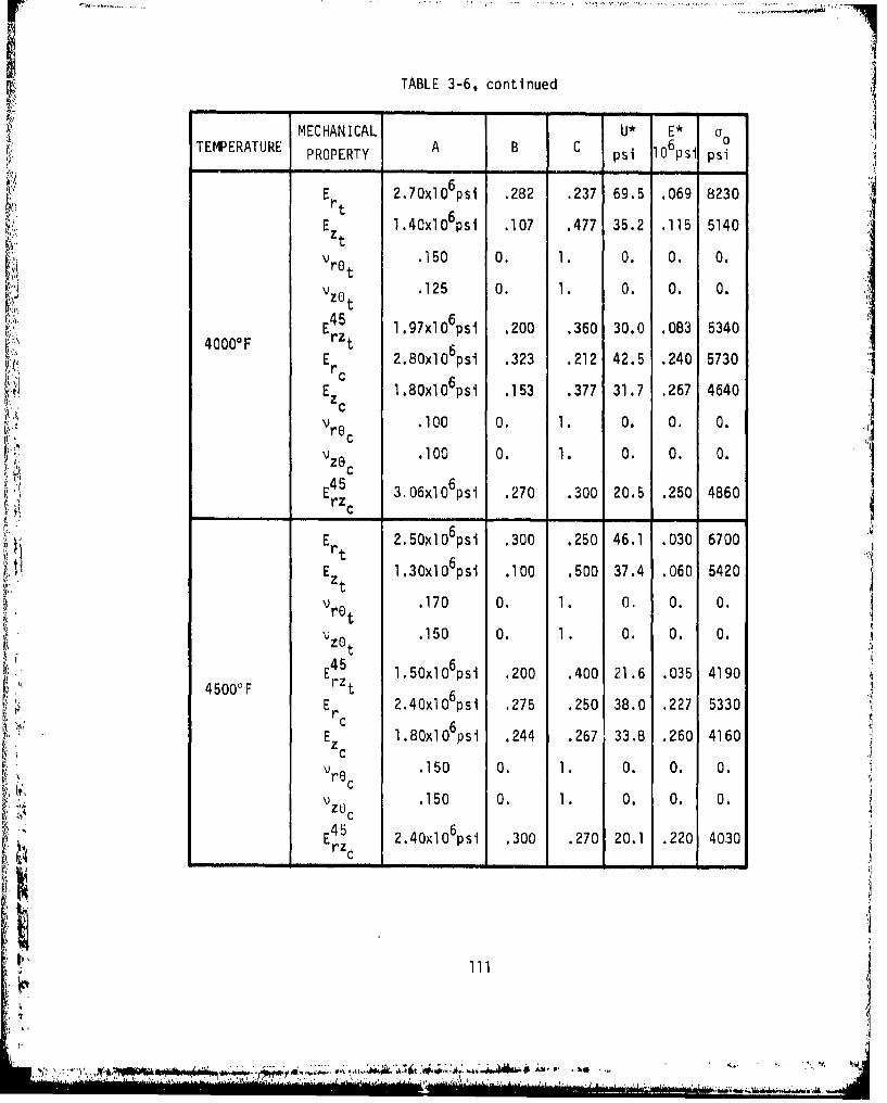
3-6 JONES-NELSON-MORGAN NONLINEAR MATERIAL MODEL PARAMETERS

FOR ATJ-S(WS) GRAPHITE AS A FUNCTION OF TEMPERATURE ........... 109

3-7 COEFFICIENTS OF THERMAL EXPANSION FOR ATJ-S(WS) GRAPHITEAS A FUNCTION OF TEMPERATURE .................................. 112

3-8 PREDICTED STRESSES AND STRAINS IN ELEMENT 232 ................. 121

"3-9 PREDICTED STRESSES AND STRAINS IN ELEMENT 134 .............. 121

3-10 ELASTIC STRESSES IN ELEMENT 232 CALCULATED WITH

DOASIS AND SAAS IIIM .......................................... 123

3-11 ELASTIC STRAINS IN ELEMENT 232 CALCULATED WITH

DOASIS AND SAAS IIIM .................... ............... 123

3-12 NONLINEAR STRESSES IN ELEMENT 232 CALCULATED WITH


3-13 NONLINEAR STRAINS IN ELEMENT 232 CALCULATED WITH


4-1 STIFFNESSES OF SANDIA CVD CARBON FELT ......................... 156

4-2 STIFFNESSES OF AVCO 3D THORNEL/PHENOLIC ....................... 156

01A xii.

I I IIIII IIII I ' --............... '....'--.................................................................

TABLES, continued

4-3 STRENGTHS OF SL\NDIA CVD CARBON FELT ........................... 163

4-4 STRENGTHS OF AVCO 3D THORNEL/PHENOLIC ......................... 163

×xiv

'., *1

I. INTRODUCTION

Artificial graphitic materials have been used for more than the

past decade in reentry vehicle nosetips. The exacting requirements im-

posed in their use necessitate accurate stress analysis techniques. An

integral part of every stress analysis is the stress-strain relationship

or material model.

The stress analysis problems inherent to reentry vehicle nosetip

design were discussed by Jones [1-1] in 1967 along with numerous specif-

ic problems by other authors in the same conference proceedings volume.

Since that time, periodic reviews of nosetip stress analysis technology

have been made. The most recent review by Jones and Koenig [1-2] is

addressed tu the material modeling characteristics necessary for graphite

and carbon-carbon. Two of the significant deficiencies of current mate-

rial modeling that they point out are (1) biaxial softening and (2) dif-

ferent moduli under tensile loading than under compressive loading.

These characteristics are described along with other characteristics of

graphite and carbon-carbon in the following paragrapns.

1.1 BIAXIAL SOFTENING

Biaxial softening is characterized by the development of slightly

larger strains in biaxial tension than in uniaxial tension, as shown in

Figure 1-1. This behavior of generally decreasing Poisson's ratios is

in contradiction to what might be anticipated on the basis of conven-

tional Poisson effects (where v increases). This phenomenon was apparent-

ly first observed by Jortner [1-3 thru 1-6] for graphite and is attri.-

buted to plastic volume changes resulting from internal tearing or micro-

cracking. Jones and Nelson [1-7] developed a material model for descrip-

4"

FiBIAXIALHARDENIING--•

(v INCREASIN G) •'

/ -- UNIAXIAL 41

BIAXIALSOFTENING

( uDECREASING) ,

ErFIGURE 1-1 BIAXIAL SOFTENING OF GRAPHITE

tion of the deformation behavior of ATJ-S graphite under biaxial tension.

Their model is used in the SAAS III program to obtain predicted strains

for Jortner's biaxial test specimen shown in Fig. 1-2. The predicted

strains are shown along with Jortner's experimentally observed strains

in Figure 1-3 for room temperature behavior at a constant principal

stress of 3550 psi. The Jones and Nelson strain predictions are within

3% of the equal biaxial tension strains and are identical to the two

uniaxial tension cases.

Actually, the Jones-Nelson model is more a general model for non-

linear behavior of orthotropic materials than just a biaxial softening

model. Thus, the Jones-Nelson model should be considered for use in

,..,,2

......................... .... ,.

1.01 1.68

CIRCUMFERENTIAL-!4.00

FIGURE 1-2 HOLLOW GRAPHITE BIAXIAL SPECIMEN

10(1:1.26)

AXIAL.003 jDT

O0 EXPERIMENTAL DATA

.002 , -- TREND OF DATASx SAAS 11

I ..-.TREND OF SAAS II.001 A IA NEW MATERIAL MODEL

-.001 .001 1.003 .004 .005

(0:) CIRCUMFERENTIAL

-.001

FIGURE 1-3 BIAXIAL STRAIN RESPONSE OF A HOLLOW ATJ-S GRAPHITE SPECIMEN

AT ROOM TEMPERATURE (700 F) AND 3550 psi PRINCIPAL STRESS

3

modeling other materials. Specifically, carbon-carbon will be shown to

be a nonlinear orthotropic material, and the basic Jones-Nelson model

will be proposed for analysis of carbon-carbon.

1.2 DIFFERENT MODULI IN TENSION AND COMPRESSION

Many composite materials behave differently under tensile and com-

pressive loads. Both the elastic moduli (stiffnesses) and the strengths

in principal material property directions of these orthotropic materials

are different for tensile loading than for compressive loading. This

characteristic behavior is shown schematically in the stress-strain

curve of Figure 1-4. This phenomenon is but one of several differences

that make composite materials more difficult to analyze (and hence de-

sign) than the more common structural materials such as aluminum.

Both fiber-reinforced and granular composite materials have differ-

ent moduli in tension and compression as displayed in Table 1-1. Uni-

directional glass fibers in an epoxy matrix have compression moduli 20%

lower than the tension moduli [1-8]. For some unidirectional boron/epoxy

fiber-reinforced laminae, the compression moduli are about 15-20% larger

than the tension moduli [1-9]. In contrast, some unidirectional graphite/

epoxy fiber-reinforced laminae have tension moduli up to 40% greater than

the compression moduli [1-9]. Other fiber-reinforced composites such as

carbon-carbon have tension moduli from two to five times the compression

moduli [1-10]. Thus, no clear pattern of larger tension than compression

moduli or vice versa exists for, fiber-reinforced composite materials. A

plausible physical explanation for this puzzling circumstance has yet to

be made.

For granular composite materials, the picture is no clearer. ZTA

graphite has tension moduli as much as 20% lower than the compression

4

S ... . . • • •w. ..-. ,W:. .... ,..... ;• :••,'• .•......,, . .. .. . .. "o'"il•

TABLE 1-1

TENSION AND COMPRESSION MODULI RELATIONSHIPS

FOR SEVERAL COMMON COMPOSITE MATERIALS

FIBROUS REPRESENTATIVEMATERIAL OR MODULI

GRANULAR RELATIONSHIP

GLASS/EPOXY FIBROUS Et * 1.2Ec

BORON/EPOXY FIBROUS Ec * 1.2Et

GRAPHITE/EPOXY FIBROUS Et 1.4E.

CARBON/CARBON FIBROUS Et U 2-5EC

ZTA GRAPHITE GRANULAR Ec a 1.2Et

ATJ-S GRAPHITE GRANULAR Et - 1.2Ec

Et

EC

•;.0

FIGURE 1-4 STRESS-STRAIN CURVE FOR A MATERIAL WITH

DIFFERENT MODULI IN TENSION AND COMPRESSION

5

moduli [1-11]. On the other hand, ATJ-S graphite has tension moduli

as much as 20% more than the compression moduli 1*1-12].

Many other materials have different tension and compression moduli.

Which modulus is higher may depend on the fiber or granule stiffness

relative to the matrix stiffness. Such a relationship would influence

whether the fibers or granules tend to contact and hence stiffen the

composite. A general physical explanation of the reasons for different

behavior in tension and compression Is not yet available. Investigation

of the micromechanical behavioral aspects of composite materials may

lead to a rational explanation of this phenomenon. Until such an expla-

nation is available, the apparent behavior can be used in analyzing the

stress-strain behavior of materials. That is, even without knowing why

the materials behave as they do, we can model their apparent behavior.

Actual stress-strain behavior is probably not as simple as shown in

Figure 1-4. Instead, a nonlinear transition region may exist between

the tension and compression linear portions of the stress-strain [1-13].

The measurement of strains near zero stress is difficult to perform

accurately, but the stress-strain behavior might be as shown in Figure

1-5 wherein replacement of the actual behavior by a bilinear model is

offered as a simplification of the obviously nonlinear behavior. For

most materials, the mechanical property data are insufficient to justify

use of a more complex material model. However, one possible disadvantage

of the bilinear stress-strain curve approximation is that a discontinuity

in slope (modulus) occurs at the origin of the stress-strain curve.

Given that the uniaxial stress-strain behavior is approximated by a

bilinear representation, the definition remains of the actual multiaxial

stress-strain, or constitutive, relations that are required in structural

6I

4 '00. .,

Lm

-'. BILINEAR APPROXIMATION //

-. ACTUAL BEHAVIOR E

Ec EI I• ITRANSITION REGION

FIGURE 1-5 COMPARISON OF BILINEAR MODEL WITH ACTUAL BEHAVIOR

analysis. Over the past ten years, Ambartsumyan and his co-workers

[1-14 thru 1-171, in the process of obtaining solutions for stress analy-

sis of shells and bodies of revolution, defined a set of stress-strain

relations that will be referred to herein as the Ambartsumyan material

model. Jones [1-18] applied the model to the problem of buckling under

biaxial loading of circular cylindrical shells made of an isotropic mate-

rial. However, in application of the Ambartsumyan material model to

orthotropic materials, certain deficiencies, such as a nonsymmeitric

compliance matrix in the stress-strain relations [1-19], are apparent.

Jones [1-201 also applied modified bilinear stress-strain relations

to buckling of shells with multiple layers of orthotropic materials hav-

ing different moduli in tension and compression. His nmdifications con-

sisL of weighting tension and compression compliances according to the

7,,

.1 ----- 11

proportions of the principal stresses in order to obtain a synMietric

compliance matrix. Isabekian and Khachatryan [1-21] made the Ambartsumyan

material model have a symmetric compliance matrix by enforcing certain

relations between the material properties. Both Jones' and Isabekian

and Khachatryan's relations are used in the modified Jones-Nelson model,

but only Jones' weighted compliance matrix material model is used in the

present report.

When the different moduli in tension and compression characteristic

is combined with the biaxial softening characteristic, the Jones-Nelson

material model leads to predicted versus experimental strains shown in

Figure 1-6. There, the predicted strains in the mixed tension and com-

pression quadrant are within 3 to 9% of the measured strains at room

temperature for the data shown. Similar, but less accurate, results

(from 9-12% error) are shown for 2000OF in Figure 1-7. The experimental

data in Figure 1-7 are much less accurate than the data in Iigure 1-6

because of testing difficulties at elevated temperatures, Thus, the

Jones-Nelson graphite material model is validated by favorable compari-

son with a well-defined set of biaxial experimental data.

1.3 CHARACTERISTICS OF GRAPHITE

Graphites used in reentry vehicle nosetips are macroscopically

homogeneous, transversely isotropic, and generally fail in a brittle

manner. The typical stress-strain curve shown in Figure 1-8 is non-

linear to failure. A typical initial modulus versus temperature rela-

tionship is also shown in Figure 1-8. There, the modulus actually in-

creases from its room temperature value until a temperature of about

3500°F is reached and subsequently decreases to nearly zero as graphite

approaches sublimation. In addition, at all temperatures, the axial

8

.005.0(1:0)

0 o

5EAXIAL :1.26) EXPERIMENTAL DATA

.003 ( BILLET 1CO-150 BILLEr 3R9-33A BILLET 16K9-27

.02V BILLET 10V9-27•, .002

THEORETICAL PREDICTIONS)+TOTAL ENERGY.001oo 0 WEIGHTED ENERGY

DIVIDED ENERGY

,.001 .001 .002 .003 .004 .0051 0I (0 :A0 (0:1) ECIRCUMFERENTIAL

-. 001

-.002

-.003 O (-.64:1)+

-004o (-1:0)

t-.OOS + (-1:1)+W,7

""-.006

"FIGURE 1-6 BIAXIAL RESPONSE OF A HOLLOW ATJ-S GRAPHITE SPECIMEN

AT ROOM IEMPERATURE (70°F) AND 3550 psi PRINCIPAL STRESS

• .3

9~

,Nq

.004

S(1:0).003 - ) C

EAXtAL o0 CaO)(:.0

(1:1.35) o o

.002(- EXPERIMENTAL DATA0 BILLET ICO -15

THEORETICAL PREDICTIONS+- TOTAL ENERGY

.001- Ow WEIGHTED ENkRGYDIVIDED ENERGY

S INPUT

-. 001 .001 .002 .003 .004i ' I I I

ow (0:1) ECIRCUMFERENTIAL

* -. 001-

-. 002-

-. 003-

0," •11:0) ow 0-:11.,-.004- (-1:

+

-. 005

FIGURE 1-7 BIAXIAL RESPONSE OF A HOLLOW ATJ-S GRAPHITE SPECIMEN

"AT 2000'F AND 3550 psi PRINCIPAL STRESS

10

I1 0 '

I0Or 3000°

•_•.4000°700~50000

2 ,

OE

E CIRCUMFERENTIAL

106psi i 1 I2 6 AND RADIALAXI.AL \ (WITH GRAIN)

(ACROSS GRAIN)

0 1 2 3 4 5 6 7

3 0T, 103 F

FIGURE 1-8 GRAPHITE BEHAVIOR

modulus is lower than the modulus in the circumferential and radial

directions.

Graphite, as mentioned previously, exhibits the biaxial softening

phenomenon and has different moduli and stress-strain curves in tension

than in compression. These characteristics were successfully modeled

by the Principal Investigator in Air Force Contract F33615-73-C-5124.

However, the temperature-dependent characteristic has not yet been

coupled to the other characteristics nor has an actual nosetip been

analyzed.

'14

,.,. .• '. .4

1.4 CHARACTERISTICS OF CARBON-CARBON

Carbon-carbon materials used in reentry vehicle nosetips are macro-

scopically inhomogeneous because of large fibers in the axial direction

of the nosetip. These materials can be characterized as orthotropic

if the fibers are in orthogonal directions, but are anisotropic if fibers

at other than 90 angles are inserted. Carbon-carbon fails in a pro-

gressive manner as illustrated in Figure 1-9. There, the material is

stressed in the direction of axial fibers which apparently slip relative

to the matrix material as stress is applied. The initial modulus versus

temperature relationship is also shown for the circumferential and radial

directions in Figure 1-9. The three curves shown are interpretations of

the same experimental data by different people. Thus, considerable dis-

agreement exists as to the actual modulus versus temperature relation-

ship. The axial modulus for this particular carbon-carbon material is

about twice the circumferential modulus. Such a relation (quite dif-

ferent from graphite) is not unexpected when the large fibers in the

axial direction are considered.

Carbon-carbon, like graphite, exhibits different moduli in tension

than in compression; however, the differences are strikingly greater

for carbon-carbon than for graphite. No evidence currently exists that

carbon-carbons exhibit the biaxial softening phenomenon. Some of the

specific mechanical properties of carbon-carbon are given by Legg,

Starrett, Sanders, and Pears [1-22].

The most evident difference of carbon-carbon from graphite is its

three-dimensional woven character as upposed to the fine-grained struc-

ture of graphite. The fibers in carbon-carbon are placed in three mutu-

t' 12

3500~

700

45000

CIRCUMFERENTIALAND RADIAL 5500

2Er

L AXIAL

EI1o6 psi1

EAXIAL 2' 2E~e)

0 1 2 3 4 5 6 7

T, 103 OF

FIGURE 1-9 CARBON-CARBON BEHAVIOR

13

S• 1 3

ally perpendicular directions. Thus, carbon-carbon is a highly ortho-

tropic material in the r-O plane of a nosetip (as opposed to the isotropy

of graphite in this plane). Geiler [1-23] used a linear elastic model

in the ASAAS program due to Crose [1-24] to account for the circumfer-I; entially varying orthotropy. Geiler obtained apparently good results.

However, the ASAAS program would be very difficult to adapt to nonlinear

analysis because of the already highly coupled, time consuming internal

workings of the computer program.

A related characteristic of carbon-carbon is that the size of the

fibers is not negligible in comparison to the ;ize of the billets in•'

which it is manufactured or in comparison to the critical dimensions of

the nosetip into which the billets are machined. (Note the Z-direction

fibers are the white streaks in the axial direction of the nosetip in

Figure 1-10,) Another way of saying the same thing is that the fiber

spacing is of the same order of magnitude as the distance over which the

41

FIGURE 1-10 CARBON-CARBON PLUG NOSETIP

14

i-,

Si ... ..... i

stresses change rapidly. Thus, we would anticipate possible difficulties

in applying a macromechanical or continuum mechanics model to carbon-

carbon materials. Not enough work has been done, however, to resolve

or even clarify the macromechanics versus micromechanics issue.

1.5 STATEMENT OF THE PROBLEM

Two principal efforts are involved in this research: one on graph-

ite material modeling and the other on carbon-carbon material modeling.

The graphite modeling is essentially a continuation of efforts begun

under Air Force Contract F33615-73-C-5124. In that contract, graphite

multiaxial stress-strain behavior was successfully modeled under both

biaxial tension and mixed tension and compression load at room tempera-

ture and at 20000 F. The remaining tasks include (1) incorporating a

temperature-dependent character in the material model (previously men-

tioned results are for a constant temperature), (2) validating the model

by comparison with further experimental data, and (3) exercising the

model in a thermostructural analysis of an actual reentry vehicle nose-

tip. Upon completion of these tasks, the graphite material model should

be ready for routine use in Air Force reentry vehicle nosetip analysis.

The carbon-carbon modeling is a new effort with the objective of

applying the basic concepts of the successful graphite model to the analy-

sis of carbon-carbon stress-strain behavior. Generally, carbon-carbon

stress-strain curves are more jagged than those of graphite. Thus, some

modifications *to the graphite model are anticipated. The first step in

carbon-carbon modeling is to describe and evaluate the stress-strain

curve characteristics. Next, a revised model will be formulated based

on these characteristics and on discussions with researchers who have

been dealing with carbon-carbon for some time (at Southern Research

15

Institute, McDonnell-Douglas, AFML, SAMSO, Prototype Development Asso-

ciates, arid Weiler Research, Inc.). The model will then be correlated

with available experimental data in a validation stage. If the model

does, or can be refined enough to, give good correlation with experi-

mental data, then the model will be evaluated for implementation in AFML

and SAMSO nosetip thermostructural analysis computer programs.

1.6 STATEMENT OF RESEARCH

The present research is divided in two rjor phases, graphite and

carbon-carbon, each of which are further divided as follows:

Phase G - Graphite

G-I - Model Formulation

G-II - Correlation

G-III - Nosetip Demonstration

G-IV - Implementation

G-V - Reporting

Phase C -Carbon-Carbon

C-I - Data Evaluation

C-If - Model Formulation

C-Ill - Correlation

C-IV - Implementation

C-V - Reporting

These phases are described in the following paragraphs.

1.6.1 PHASE G - GRAPHITE

Phase G-I - Model Formulation

The graphite material model has but one essential characteristic to

be incorporated prior to use in actual nosetip analysis. That charac-

16

2 t I! ' i "i y I

teristic is temperature-dependent material behavior. A new scheme must

be devised to express the material model as a function of temperature

based on data at a finite number of temperatures. Basically, the objec-

tive is a material property versus temperature interpolation scheme.

However, this scheme is complicated by the presence of many more mate-

rial property characterization constants in the present model than in

previous models for which such interpolation is well-known.

Phase G-II - Correlation

The graphite material model will continue to be correlated with

available experimental data. All known biaxial data generated on con-

stant temperature tube specimens by Jortner of McDonnell-Douglas has been

successfully correlated. The next logical step is to attempt correla-

tion with data on specimens with a nonconstant temperature, i.e., a

temperature gradient. The data for the wedge-shaped disc shown in Figure

1-11 generated in the Temperature/Stress Test developed by Southern

.071" R

-. 500" 1.625"

- ý[-.375`,

I 'l

FIGURE 1-11 WEDGE-SHAPED DISK SPECIMEN

17

Research Institute [1-25] is most appropriate. Limited correlation

studies will be performed with that data. Calculated temperature pro-

filges (verified by measurement) through the disc will be used in con-

junction with the temperature-dependent material model to predict

disc diameter changes. These predictions will be compared with Southern

Research Institute measurements to further validate the material model.

Phase G-III - Nosetip Demonstration

The final stage in the development of the material model is to exer-

cise the model in thermostructural analysis of a reentry vehicle nose-

tip. Although "experimental" data are limited (obviously only flight

tests with limited instrumentation can be considered experiments in the

present context), the comparison of predictions of the present model with

previously used models is essential. Without such comparisons, the real

worth of the present graphite material model for reentry vehicle nosetip

stress analysis cannot be established.

The finite element data cards for the nosetip and its thermal (and

mechanical) loading will be chosen by AFML and supplied to Southern Meth-

odist University in the SAAS III format. These data cards shall have

been previously verified to work on SAAS III by another contractor for

an all-elastic analysis or an elastic-plastic bilinear analysis. Accord-

ingly, the nosetip demonstration will involve a single variable, the

material model. All other variables will be provided to SMU in ready-to-run form.

Phase G-IV - Implementation

"The graphite material model developed and validated in previous

phases and in Air Force Contract F33615-73-C-5124 will be incorporated

in a version of the SAAS III computer program [1-26]. That program is

18

.. . ..1' . , , . . . .. • , • €..• .',• ••• .,,.•,l,¶ .,,,.. .,,,.•• • :,,• •.••., ,.,,• ,d,,• •, . .,, , ...

the basic finite element computer program operational at Southern

Methodist University. Duplicate computer decks, listings, test cases,

and output will be provided to AFML should an operational deck be de-

sired. In view of Southern Methodist University's mission of graduate

education and research, limited manpower, and small computer, the graph-

ite material model will not be implemented in any program other than

SAAS III.

Phase G-V - Reporting

The graphite material modeling efforts, correlation studies, and

nosetip analysis are de~scribed in the present Technical Report.

1.6.2 PHASE C - CARBON-CARBON

Phase C-I - Data Evaluation

Carbon-carbon materials have many different manufacturing processes

and hence many different characteristics, as alluded to earlier. The

objective of the data evaluation phase is to examinE the available mate-

rial property data and isolate the significant characteristics that must

be modeled to accurately predict thermostructural response. This objec-

tive will be met by review of published data, review of published mate-

rial modeling efforts, and consultation with AFML, SAMSO, Southern Re-

search Institute, McDonnell-Douglas, Prototype Development Associates,

and Weiler Research, Inc. The latter consultation should take place both

in this phase and in subsequent phases. Because of this consultation

and the expectatio•n that important material properties will likely be

found to not have been measured, data evaluation will be regarded as a

phase continuing thrnughout the remainder of the program.

Phase C-If - Model Formulation

The basic material model used for' graphite and described in Reference

I Y

!.'19

'!'

•J

1-7 will be fit to the thermostructural characteristics of carbon-carbon.

Should a more complicated relationship be necessary, studies will be ini-

tiated to determine an appropriate relationship.

The behavior of carbon-carbon will be studied in this initial effort

from the standpoint of the axisymmetric macromechanics or continuum me-

chanics analysis in SAAS Ill [1-26]. In addition to the basic SAAS III

analysis with the new material model, an essentially one-element model

with the new material model will be used in modeling feasibility studies

such as were carried out in Air Force Contract F33615-73-C-5124. Neither

the asymmetric linear elastic analysis of ASAAS [1-24] nor micromechan-

ical analyses will be attempted. Evaluation of the need for and benefit

from more geometrically sophisticated models will be made in conjunction

with the data evaluation phase. That is, we must be certain the quality

and sophistication of the data merit the increased expense of, e.g.,

asymmetric micromechanical analyses.

Carbon-carbon will be modeled in uniaxial on-axis and off-axis

stress states for which material property data exist. Moreover, limited

biaxial stress state data will also be modeled to the level of sophisti-

cation possible within the scope of two-dimensional or axisymmetric macro-

mechanics theory.

Phase C-Ill - Correlation

The material model developed in the previous phase will be used toA

obtain stress-strain predictions for situations in which carefully ob-

tained experimental results are available. These experimental data will

be selected in cooperation with AFML. These experiments will include

:. uniaxial on-axis and off-axis tests, the most logical starting point for

any material modeling effort. In this manner, the material model will

20

' ..4 ',. ., . . . , . + ., . ,

4.r

either be validated by comparison with experimental data or will be in-

validated and improvements will be made.

Phase C-IV - Implementation

The carbon-carbon material model developed and validated in previous

phases will be incorporated in a version of the SAAS III computer pro-

gram [1-26]. That program is the basic finite element computer program

operational at Southern Methodist University. This research program is

not likely to advance the state of the art of carbon-carbon modeling to

the point where the model is judged completely ready for widespread Air

Force use in reentry vehicle nosetip stress analysis. Instead, the

present effort is best described as a bold step toward that goal with

some hope of a reasonable model being obtained within the next year.

Southern Methodist University expects that further work on carbon.-car-

bon modeling will be necessary before the real question of implementation

of the carbon-carbon model in Air Force computer programs arises.

"P"hase C-V - Repor.ng

The carbon-carbon material modeling studies, including data evalua-

tion and characterization, model formulation, and correlation activities,

are described in the present report.

1.7 SCOPE OF REPORT

The actual accomplishments during the contract are presented in the

following sections. First, the Jones-Nelson nonlinear material model is

reviewed in Section 2. Also, that model is extended to temperature-de-

pendent material behavior and to treatment of extrapolated stress-strain

curves in what is called the dones-Nelsor-Morgan model. Then in Section

3, the graphite modeling efforts are described. First, the correlation

A ' 21

I,

..............,... .,..... •,. ..... .. '

studies for the Southern Research Institute thermal stress disk test are

discussed. Then, the AFFDL 50 MW nosetip correlation studies are de-

scribed. The carbon-carbon modLling efforts are discussed in Section 4.

The general modeling is first described and then a characteristic of

carbon-carbon in bending tests is treated. The current contract efforts

are summarized in Section 5.

t.I

)IrII

!" 22

2. JONES-NELSON-MORGAN NONLINEAR MATERIAL MODEL

2.1 INTRODUCTION

First, the basic Jones-Nelson nonlinear material model is briefly

reviewed in Section 2.2, and some new aspects o'F its behavior are de-

scribed. In particular, procedures are developed for temperature inter-

polation of temperature-dependent material behavior. Then, methods of

extending the range of applicability of the material model are discussed

in Section 2.3. The major accomplishment in that section is the develop-

ment of an extended stress-strain curve version of the Jones-Nelson model

which is called the Jones-Nelson-Morgan nonlinear material model. Final-

"ly, the JNMDATA computer program is described in Section 2.4. This pro-

gram is used to convert the various measured stress-strain curve data

directly to the parameters of the Jones-Nelson and Jones-Nelson-Morgan

material models suitable for use in the SAAS HIM finite element stress

"analysis computer program which is a modification of the SAAS III pro-

gram [2-1]. The JNMDATA program is a very useful aid in the modeling of

a material because the results are obtained automatically and are pre-

sented visually for rapid evaluation of the model.

2.2 JONES-NELSON NONLINEAR MATERIAL MODEL

The Jones-Nelson nonlinear material model was developed under USAF

Contract F33615-73-C-5124 and reported in AFML-TR-74-259 [2-2]. Several

other related and more accessible publications are condensed from Ref.

2-2, namely Refs. 2-3 thru 2-6. That work will be summarized in Section

2.2.1 for the sake of convenience in reading this report. The necessary

further details will be referenced where required. Then, a new discus-

sion of how to implement the model is presented in Section 2.2.2. There,

23

" " "••wdl • • ' e•'v• • ....... ,. ,•,.,Jw• .•w• '•, ,,.•. ,, ,•. '~w,, ,,a...Lv...• ,,'r, i '

the recent experience in application of the model is reflected. Finally,

the model is extended in Section 2.2.3 to interpolation of temperature-

dependent material behavior at temperatures between available data.

2.2.1 BASIC APPROACH

The basic problem is the stress analysis of nonlinear elastic bodies

whose stress-strain behavior is described with, for the example of an

orthotropic axisymmetric body under axisymmetric load, the equations:

1 Vrz VrO

rr r r

rz 1 az•z r• Qz z

(2.1)Vre VrO 1 0

Er z 0

Yrz 0 0 0 G Trzrz

where the directions denoted with the subscripts r, z, and 0 are princi-

pal material directions. The material properties in the compliance ma-

trix of Eq. (2.1) are

Er = Young's modulus in the r direction

Ez = Young's modulus in the z direction

E0 = Young's modulus in the 0 direction

V rz C z/ r for the loading ar a (all other stresses zero)

r -Eo/C r for the loading ar y (all other stresses zero)

V -•O/Iz for the loading uz a (all other stresses zero)

Grzo Shear modulus in the rz plane

24

.'

• | . . , . •,, • m~m wi• w-•- .,( r•..,,L... .. , .,, • ,i • .'• J'''''' ' • • •' .. ... .. "

The reciprocal relations of orthotropic elasticity

Vrz /Er Vzr /Ez Vro /Er vor/E0 Vze /Ez O oz/Ee (2.2)

can be used to express alternative definitions for the Poisson's ratios

in terms of the seven independent material properties in Eq. (2.1). The

material properties in Eq. (2.1) are a function of stress level because

the material is nonlinearly elastic. However, we do not examine the

unloading behavior nor any subsequent reloading behavior of the body.

The basic stress analysis problem could be more complicated than is

represented with Eq. (2.1). For example, the material could have prin-

cipal material directions at some angle to the r-z-6 coordinate system.

Or, the material could have different stress-strain behavior in tension

than in compression. The stress-strain relations for multimodulus mate-

rials are derived by Jones and Nelson [2-2, 2-5] and are applied to stress

analysis of graphitic materials in Ref. 2-6. The foregoing considerations

are obviously more complicated than what is represented with Eq. (2.1).

However, those equations will suffice for our discussion of the Jones-

Nelson material model.

The basic premise of the Jones-Nelson nonlinear material model is

that the mechanical properties of a material, e.g., the material prop-

erties in Eq. (2.1), are expressed in terms of the strain energy of the

body with the approximate equation

Mechanical Propertyi Ai[l - Bi(U/Uloi)i] (2.3)

where the Ai are the elastic values of the material property, the Bi andE• i

Ci are related to the initial curvature and rate of change of curvature,

respectively, of the stress-strain curve [2-2, 2-4] (slightly different

25

*.k~~*-' ~A~q ..

•' " .. • •," !,~ •,, • .. •. ,,., , . ..... . .... ; ,• :,; , . , •.... ... ,W,., .. .. . • ,." " "

interpretations exist when the mechanical property is a Poisson's ratio),

and U is the strain energy density of an equivalent elastic system at

each stage of nonlinear deformation:

U = (Orer + QzCz + 0 + trzYrz )/2 (2.4)

The strain energy density U is normalized by Uo0 in Eq. (2.3) so that Bii1

and Ci are dimensionless. Typical stress-strain curves, the correspond-

ing mechanical property versus strain energy curves, and the associated

mechanical property equations for a Young's modulus and a Poisson's ratio

are shown in Fig. 2-1.

The nonlinear stress-strain model is actually much more complicated

than Eq. (2.3). When mixed tensile and compressive stresses are excited,

the strain energy used in Eq. (2.3) could be a weighted combination of

the strain energy of compression and that of tension. Moreover, all

coefficients have different values in tension than in compression. The

choice of which properties, tension or compression, should be used is

made in the Ambartsumyan superposition manner [2-7] after rotating the

stress-strain relations to principal stress directions as described in

Ref. 2-2.

The stress-strain relations, Eq. (2.1), and the mechanical property

versus energy equations, Eq. (2.3), are a set of indeterminate relations

which are solved with the iteration procedure shown in Fig. 2-2. That

is, the stresses and strains depend on the mechanical properties (through

Eq. 2.1) which, in turn, depend on the stresses and strain [through Eqs.

(2.3 and (2.4)]. The determination of mechanical properties and, con-

sequently, the stress-strain relationships is based on both the propor-

tions of the principal stresses and on the magnitude of an energy func-

26

5 2.5

4 2

STRESS E103 psi 3 /iEC

10 psi .5

2~~ EE1ESECe 2(lQ0[1-.2(y )

1 .5 1-0 ' L II I 0 , I _

0 .001 .002 .003 .004 0 5 10

STRAIN STRAIN ENERGY, U, psi

(a) DIRECT MODULUS

AXIAL STRESS1.0 3 psi

44.1

.2 .03 4

ETRANSVERSE EAXIAL

-.0004 V o .004 0 5 10STRAIN STRAIN ENERGY, U, psi

S(b) POISSON'S RATIO

FIGURE 2-1 REPRESENTATION OF STRESS-STRAIN RELATIONS

FOR DIRECT MODULI AND POISSON'S RATIOS

27

2).

1EXPRESS MATERIAL PROPERTIES IN TERMS OF TOTAL ENERGY U FROM UNIAXIAL DATA

FORM COMPLIANCE MATI IN M 1TH

INITIAL LINEAR TENSION VALUES OF MATERIAL PROPERTIES1

ICALCULATE STRESSES, STRAINS, AND STRAIN ENERGYI

FCALCULATE NEW MATERIAL PROPERTIES~s

.FORM ALL-TENSION AND ALL-COMPRESSION COMPLIANCE MATRICES IN PMD.

.ROTATE COMPLIANCE MATRICES TO PSOI

[FORM MULTIMODULUS COMPLIANCE MATRIXIN PS0

iV",CALCULATE NEW STRESSES, STRAINS, AND STRAIN ENERGY

EVALUATE REL AU -(u"U 1-U1)/U 11ý

IFIREL AUI < SPECIFIED VALUE, STOP iREL AU, > SPECIFIED VALUE

PMD - PRINCIPAL MATERIAL DIRECTIONS

PSD - PRINCIPAL STRESS DIRECTIONS

FIGURE 2-2 ITERATION PROCEDURE FOR NONLINEAR MULTIMODULUS MATERIALS

* .,I 4 q .~ .... •, I,, ...... w. ;1

tion. Each step in the iteration procedure is described in Refs, ?-2

and 2-5.

Two different energy functions - total strain energy and weighted

strain energy - can be used in the Jones-Nelson material model. The

total strain energy is defined in Eq. (2.4). On the other hand, in 'the

weighted strain energy, the total strain energy is separated into two

components: (1) the contribution from the tensile principal stresses

and (2) the contribution from the compressive principal stresses. Then,

the effective energy level, Uw, in terms of the tension and compression

components of the total strain energy is

Uw (Ut 2 + Uc2 )/U (2.5)

This energy Uw is used to determine both the tension and compression

material properties.

2.2.2 IMPLEMENTATION OF THE MATERIAL MODEL

Much of the work in implementing the Jones-Nelson nonlinear mate-

rial model is in calculating appropriate values of A, B, and C in the

governing equation, Eq. (2.3). To reach the point where these calcula-

tions can be made, we must first determine the secant values of the me-

chanical properties and the corresponding values of strain energy from

uniaxial stress-strain curves of the material under investigation. For

example, the values of the secant shear modulus and corresponding values

of U can be determined from a shear stress - shear strain curve such as

shown in Fig. 2-3. There, for two shear stress levels, the correspond-

ing shear strains are found from the experimentally determined shear

stress - shear strain curve. Then, Gl2 and U are calculated from

'1.29

I. 4 .i q_,.

1I2

2 2

T 1 2 , 7I

U2

FIGURE 2-3 NONLINEAR SHEAR STRESS -SHEAR STRAIN CURVE

G12 -'I (2.6)sec ~l

U -12Y12/2 (2.7)

Similarly, the remaining secant mechanical properties and their corres-

ponding strain energies are found from the appropriate stress-strain

curves in principal material directions.

Next, all secant mechanical properties are plotted versus the strain

energy as in Fig. 2-4. Now, we can begin to calculate or otherwise find

the values of A, B, and C in Eq. (2.3). First, the constant A is the

initial (elastic) value of the mechanical property. That is, it is the

initial slope of the stress-strain curve in Fig. 2-3 or the intercept of

the mechanical property versus energy curve in Fig. 2-4. The value of A

is higher than you would expect from the normal procedure of placing a

30

. ,q� ... . .... .... •,_• __,4 ,

DDATA POINT USED TO DVER~tMINE A

1FA A P I T S D T "MECHANICAL -DATA POINTS USED

PROPERTY T0 DETERMINE & C

2A

3

$TRAIN INEROY, U

FIGURE 2-4 REPRESENTATIVE MECHANICAL PR~OPERTY VERSUS U CURVE

Kstraightedge on a stress-strain curve such as Fig. 2-3. We draw this

conclusion on the basis of many observed fits of the material model to

stress-strain curves with simultaneous fits to a corresponding mechani-

cal property versus energy curve. That is, the curve on a plot of me-

chanical energy versus energy "heads" for a much higher intercept at

ULO than you would expect from looking at the stress-strain curve alone.

This conclusion is not surprising when viewed in the context that the

mechanical property is the slope (first derivative) of the stress-strain

curve and hence is a more sensitive indicator of the behavior when

plotted against energ~y than when visually determined from a necessarily

somewhat inaccurate stress-strain curve.

The constants B and C are determined from data at two points on the

material property versus U curve as shown in Fig. 2-4. The values of the

A mechanical property and the values of U at these two data points are sub-

stituted In Eq. (2.3). Two equations in the two unknowns, B and C, re-

suit. These two equations are solved simultaneously for B and C to get

31

A -(M .P . ) 2-log L . .M P ) _

c U (2.8)

B - u (2.9)

where (M.P.) 2 and (M.P.) 3 are the values of the mechanical property at

the two data points chosen from the mechanical property versus U curve.

The values U2 and U3 in Eqs. (2.8) and (2.9) are the strain energies at

the two chosen data points. The proper choice of data points from the

mechanical property versus U curve is an important part in the applica-

tion of the material model to a specific material and will be discussed

next.

The use of Eq. (2.3) to approximate each mechanical property

corresponds to the mathematical procedure of three-point interpolation.

At the three data points used in determining A, B, and C, the approximatevalues of the mechanical property are the same as the actual values. In

the region between these three points, Eq. (2.3) is a reasonable approxi-

mation of the mechanical property versus strain energy data. Thus, an

interval of strain energy for which Eq. (2.3) is a valid representation

of the mechanical property is defined by the positions of points 1 and

, I3 in Fig. 2-4. This interval of strain energy is bounded on the left by

,U=O, the strain energy at point 1, and on the right by the strain energy

at point 3. The approximate mechanical property versus U curve must pass

1? through point 2 so the shape of this curve between points 1 and 3 is de-

termined from the position of point 2. Obviously, more information than

32

L 4*'dW ,&i$ l*f .

just data to calculate B and C is gained about the mechanical property

approximation from the data points 1, 2, and 3 in Fig. 2-4. The func-

tions of these points can be summarized as follows:

(a) Point 1 is used to determine the constant A in Eq. (2.3) and

is the left bound of the interval of strain energy for which

the approximate mechanical property versus U curve is valid.

(b) Point 3 is used in determining B and C in Eq. (2.3) and is

* the right bound of the interval of strain-energy for which the

approximate mechanical property versus U curve is valid.

(c) Point 2 is also used in determining B and C in Eq. (2.3), and

the shape of the approximate mechanical property versus U curve

is defined by the position of point 2 in the interval between

points 1 and 3.

The choice of data points used to determine B and C is quite impor-

tant. If B and C are calculated from data at points 2 and 3 on the actual

mechanical property versus strain energy curve (solid line) in Fig. 2-5,

the dashed-dotted curve labeled 2-3 is the result. This curve Is a rea-

sonable representation of the actual data in the interval 0 < U < U3

where U3 is the value of the strain energy at point 3. For strain ener-

gies larger than U3, the "2-3" curve does not and is not supposed to re-

present the mechanical property versus strain energy behavior accurately.

The mechanical property equation is valid over a larger interval of

strain energy if a point further out than point 3 on the actual mechani-

cal property versus U curve is used in the calculation of B and C. For

example, when point 4 is used in determining B and C, Eq. (2.3) is valid

-in the interval 0 < U < U4 where U4 is the value of the strain energy

at point 4. Both the "2-4" curve (B and C determined from data at points

33

,- .h

I :I

ACTUAL DATA

MECHANICALPROPERTY

2 4

2-3

I IU2 U3 U4

STRAIN ENERGY, U

FIGURE 2-5 REPRESENTATIVE MECHANICAL PROPERTY VERSUS U BEHAVIOR

AND POSSIBLE APPROXIMATIONS

2 and 4) and the "3-4" curve (B and C determined from data at points 3

and 4) in Fig. 2-5 are reasonable approximations of the actual mechanical

property versus strain energy data for 0 < U < U4 . However, in the in-

terval 0 < U < U3 neither the "2-4" nor the "3-4" curve are as good a

representation of the actual data as the "2-3" curve. Thus, the me-

chanical property equation is valid over a large interval of strain ener-

gy when point 4 is used in finding B and C, but the accuracy of the ap-

proximatlon in smaller subintervals of the overall interval is sacrificed.

Although the "2-4" and "3-4" curves are valid over the same interval

of strain energy, the two curves have different shapes in the interval

because different combinations of data points are used in determining B

and C. The "2-4" curve must pass through point 2 whereas the "3-4" curve

must pass through point 3. (Both curves must pass through points 1 and

34

4.) Because the mechanical property at point 3 is less thdn the mechani-

cal property at point 2 and because U3 is greater than U2 , the "3-4"

curve is steeper than the "2-4" curve for U < U2 and flatter for U > U3 .

In the interval U2 < U < U3 the two curves have basically the same shape.

As a result, the "2-4" curve is a better approximation in the interval ,

0 < U < U2 and the "3-4" curve is a better approximation in the interval IU3 < U < U4 . Obviously, in the interval U2 < U < U3 , both approximations

are about equally good; the "2-4" approximation is better for the strain

energies nearer U2 , and the "3-4" approximation is better for the strain

energies nearer U3 . The Interval U3 < U < U4 in Fig. 2-5 is larger than

the interval 0 < U e U2 so the "3-4" approximation is better than the

"2-4" approximation over a large portion of the overall 'interval of valid-

ity 0 < U < U4 . Thus, the interior data point used to determine B and

C should be chosen so that the approximate mechanical property versus U

curve takes on the shape desired by the user of the material model and

represents the actual data accurately over the desired subinterval of

the overall range of validity of the approximation.

With the criteria discussed above as a guide, the actual determina-

tion of the constants A, B, and C seems quite easy. However, measured

stress-strain data and corresponding mechanical property - strain energy

data are somewhat random by nature and do not usually plot as smooth

curves. When A, B, and C are determined without regard for the random

nature of the data, several pitfalls arise which are not obvious at first.

These problems can occur if a single set UT constants (A, B, and C) for

a single mechanical property is calculated by hand or if many sets of

constants for marry mechanical properties are calculated with the aid of

L a computer.

35

The procedure for determining A, B, and C can be quite tedious when

performed by hand calculation. The measured stress-strain data must

first be converted to mechanical property - strain energy data. Then,

a value for the conw-tant A must be determined. By definition, A is the

initial elastic value of the mechanical property, but obviously this ini-

tial value cannot be determined from the data at the origin of the stress-

strain curve (/c = 0). Hence, the initial slope of the measured stress-

strain curve, i.e., the tangent modulus at the origin of the stress-

strain curve, is often used as the value of A. An alternative approach

for finding A is to calculate the value of the mechanical property at

the data point corresponding to the lowest measurable stress-strain level

and then to arbitrarily use this value of the mechanical property as the

value of A. Thus, in this approach, a point on the mechanical property

versus U curve for which the strain energy is small is translated to the

mechanical property axis. One consequence of determining A in this manner

is that the value of A is less than the value obtained by using the ini-

tial slope of the stress-strain curve. Another consequence is that data

at this point cannot be used in the calculation of the constants B and

C. After A is found, the actual mechanical property - strain energy

data is plotted, and points to be used in determining B and C ire chosen.

Once B and C are calculated, the approximate mechanical property versus

U is plotted to ensure that a reasonable representation of the actual

data is obtained.

* For materials wiLh more than one stress-strain nonlinearity, the use

of hand calculations in determining the constants for each mechanical

property is inefficient becat;iýe of the large amount of time involved.

As a result, the procedure for determining A, B, and C should be auto-

,36

mated so that the calculations are performed by a computer and so that

the curves are plotted by an associated mechanical plotter. In the

JNMDATA computer program written for this purpose, the measured stresses

and strains are input data. The corresponding mechanical properties and

strain energies are calculated in the program, and the value of the me-

chanical property at the first input data point is used as the value of

A. The user of the program is able to specify which data points, other

than the first one, are used in determining the constants B and C. After

the constants B and C are calculated, the program is designed so that

the actual mechanical property - strain energy data and the approximate

mechanical property versus strain energy curve are plotted on the same

page. Also, the measured stress-strain data and the stress-strain curve

implied from Eq. (2.3) and calculated in the program are plotted in a

similar fashion. Checks of the input data are performed in the program

as a precautionary measure to avoid the pitfalls which arise in choosing

data points to determine B and C. These pitfalls, due mainly to the

random nature of the measured stress-strain data, are mentioned briefly

in a preceding paragraph and are discussed in detail in the following

paragraphs.

One of the pitfalls which arises if B and C are determined from an

arbitrarily chosen combination of data points 'is that the value of the I

constant C can be indeterminant. If B and C are chosen from data points

2 and 3 in Figure 2.-6a, the mechanical property at point 2, (M.P.)2, is

greater than A, and the mechanical property at point 3, (M.P. 3, is less.• ' ,

th'in A. As a result, the argument of the logarithm in Eq. (2.8) is nega-

tive so C cannot be determined. If a mechanical property versus strain

energy curve passed through points 2 and 3 in Fig. 2-6a, the correspond-

I37

L INN

2 3MECHANICAL1

(a ) PROPERTY

(M.P.) 2 > A A 3 2 /(M.P,3< A (M.R)2>A

(M.R 3 <A

STRAIN ENERGY, I E

3 0MECHANICAL 3

(b) PROPERTY

(M.P.) 2 < A

(M.P.) 3 > A (M.2)j),A

STRAIN ENERGY, U 1"

MECHANICAL(c ) PROPERTY

(M.P.) A 2 30 (M.P.) 3 " A (M3)2 ,(MR)3umA

STRAIN ENERGY, U

(d) MECHANICAL 1/PROPERTY 3(M.P.) 2 M A 1 R2 0A

(M.P.) 2 " (M'P') 3 MP) 3 "A

STRAIN ENERGY, U E

FIGURE 2-6 DATA POINTS WHICH LEAD TO PITFALLS IN CALCULATING B AND C

38

....... .,.... ""

ing stress-strain curve, also shown in Fig. 2-6a, would be initially con-

cave upward and then would become concave downward. This type of stress-

strain behavior is highly unusual and will probably never he encountered.

However, measured stress-strain data often has the characteristic that

at least one data point is out of line with the rest of the data. If

this data point is one of the points used to determine B atid C, the sit-

uation shown in Fig. 2-6a where (M.P.), is greater than A and (H.P,) 3 is

less than A is encountered. When this situation arises, the process of

finding the values of B and C, whether performed by hand or with the aid

of acomputer, should be stopped and new data points chosen.

The concave downward then concave upward stress-strain behavior in

Fig. 2-6b, like the stress-strain behavior in Fig. 2-6a, will probably

never be encountered. However, a point at which the mechanical property

is less than A, such as point 2 in Fig. 2-6b, and a point at which the

mechanical property is greater than A, such as point 3 in Fig. 2-6b.

could easily be chosen as the two data points to determine B and C, If

t "two such points are used, the argument of the logarithm in Eq. (2.8) is

again negative. The constant C is again indeterminant so the process of

calculating B and C should be stopped, and new data points should be cho-

sen.

The initially linear, then nonlinear, and finally linear stress-

. €strain behavior in Fig. 2-6c is also highly unusual but is shown to il-

lustrate a problem which occurs when P and C are determined from another

combination of data points. The mechanical property at point 2 in Fig.

2-6c is not equal to A, but the mechanical property at point 3 is equal

to A. When these data points are used in finding the values of B and C,

the denominator of the argument of the logarithm in Eq. (2.3) is zero so

39

v 1-

JI.-

C cannot be calculated. Thus, this combination of points must be avoiaedin choosing data points to use in determining B and C.

A different type of problem arises if the mechanical property at

point 2 is equal to the mechanical property at point 3 but is not equal

to A as in Fig. 2-6d. Because of random measured data, this situation

can occur, when points 2 and 3 are chosen close to each other. Fur, this

combination of data points, the constant C is zero so the approximate

mechanical property is not dependent on the strain energy. The value of

B is A - (M.P.) 2 . The approximate mechanical property is a constant but

is neither equal to A nor to the mechanical property at point 2 or point

3. That is, the stress-strain behavior in Fig. 2-6d is approximated by

a straight lire with slope less than A but greater than the value of the

mechanical property at point 2 or point 3. Thus, the condition that the

approximate mechanical property curve must pass through the three data

points used to determine A, B, and C is violated. The unusual stress-

strain curve with two linear portions of different slope in Fig. 2-6d

cannot be represented exactly. Only an approximation of the behavior, in

which the two linear portions are modeled as being nonlinear, can be ob-

tained when Eq. (2.3) is used to approximate the mechanical property.

To obtain this mechanical property approximation, point 2 i'n Fig. 2-6d

must be located on the nonlinear portion of the stress-strain curve so

that; values for B and C can be found.

Pitfalls similar to those discussed above can arise even when common

types of stress-strain behavior are modeled if the points used to deter-

mi ne B and C are chosen indiscriminately. The stress-strain behavior of

many materials is represented by the initially linear and then nonlinear

stress-strain curve in Fig. 2-7a. However, Eq. (2.3) cannot be used to

40

e

NOI• i• '" . 'I.•- • .•. '•,Zw .,h• m .• ,.,..,,•r••.q . .... ..... .. •.• .•,m • .'., *, ,•,,J0,,_6 ,,, -,I"...

0413 3 /'ý

MECHANICAL 1 2 3j 3PROPERTY (.)=2 2

(M.R) 32

r ~STRAIN ENERGY, U

(a) (M.P.)2 A. (M.P.)3 0 A

MECHANICAL 1l 2 3 3PROPERTY

(M.R')2=(M-P.)3 =A 2

STRAIN ENERGY., UE

(b) (M.P.)2 =(M.P.)3 -A

FIGURE 2-7 MECHANICAL PROPERTY VERSUS U BEHAVIORS WHICH

CAUSE DIFFICULTIES IN DETERMIN'ING B AND C

41

Wfx744

approximate the corresponding mechanical property behavior if points 2

and 3 in Fig. 2-7a are used in determining B and C. The mechanical prop-

erty at point 2 is equal to A but not equal to the mechanical property

at point 3. The constant C is indeterminant because the argument of

the logarithm in Eq. (2..8) is zero. Hence, the procedure for calculating

B and C must be stopped. This problem is avoided by choosing point 21 on

the nonlinear portion of the stress-strain curve to be used to determine

B and C instead of point 2. The implied stress-strain curve resulting

from this approximation is nonlinear at all levels of stress and strain

and is a reasonable approximation of the stress-strain curve in Fig.

2-7a, but the measured linear then nonlinear• stress-strain behavior can-

not be modeled exactly with Eq. (2.3).

Even for linear stress-strain behavior shown in Fig. 2-7b, B and C

must be determined carefully. Obviously, the value of the mechanical

property at points 2 and 3 in Fig. 2-7b is equal to A, but if B and C

are deteririned with Eq. (2.8) and Eq. (2.9), the argument of the loga-

r;thm in Eq. (2.8) is indeterminant (0/0) so C cannot be calculated.

However, linear stress-strain behavior is implied from Eq, (2.3) if B

is zero and C Is finite. Thus, the problem of C being indeterminant

is solved by skipping the calculations in Eqs. (2.8) and (2.9) and assign-

ing B the value of zero and C suane arbitrary but finite value.

With B and C determined from a proper choice of data points on the

mechanical property versus strain energy curve, the mechanical property

equation is a valid approximriation of the actual mechanical property data

over a specfied range of strain energy. However, under many loading

conditions, a value of the mechan',cal property is desired for a strain

energy larger than the maximum value of U for which the actual mecharti-

42

Criuji----------- u

UMA1 END OF DEFINED

EAXI UDIIN UMhX

FIGURE 2-8 UNIAXIAL. STRESS-STRAIN BEHAVIOR AND CORRESPONDING

MATERIAL PROPERTY VERSUS U BEHAVIOR

cal property versus U curve is defined. For example, the mechanicalproperty versus U curve in Fig. 2-8 is defined for strain energies in

the range 0 < U < Ulna x. This curve is obtained from the uniaxial stress-

strain curve also in Fig. 2-8 which is not defined for stresses greater

than 0max and strains greater than Enax" Hence, Fsec is not defined for

strain energies greater than UaX 0 maX emax/ 2. A problem arises if a

value of the mechanical property is needed for a strain energy greater

than UmaX, Thus, the actual mechanical property versus strair energy

curve must be extrapolated in some way. Two extrapolation procedures

for the material model are described in Section 2.3.

2.2.3 TEMPERATURE INTERPOLATION OF DEFORMATION BEHAVIOR

Many materials have temperature-dependent deformation behavior.

Typically, that deformation behavior is measured at discrete values of

temperature over some pnrtinment range of temperatures. We propose to

use such date in finite element stress analysis of bodies subjected to

temperatu gradients Then, the basic problem is: given two stress-

43

x

strain curves at two temperatures with associated mechanical property

versus strain energy curves for which we known A, B, C, and Uo, fina

the correct property for an intermediate temperature at a specified ener-

gy level alonyj with the associated point on the stress-strain curve for

the intermediate temperature. Repeated answering of this question for

:,ny energy levels would lead us to a mechanical property versus energy

L•urve and a stress-strain curve for the intermediate temperature. These

curves must lie appropriately between the respective two original curves

for the temperatures between which we interpolated the deformation be-

havior.

At least three approaches are possible: parameter interpolation,

property interpolation, and stress-strain curve interpolation. Each of

these approaches is defined and discussed in this section. Moreover,

the consequences of using each approach are discussed relative to what

is perceived to be the desired result. The word perceived is used

because the actual variation or mechanical properties with temperature

is often not known except, as stated before, at discrete temperatures.

That is, the actual, smooth variation with temperature of properties or

stress-strain curves is not known so we have little with which to compare

our results.

The basic example for all three approaches will involve the Inter-

polatioi of AlJ-S graphite properties at 1403OF when we are given the

properties at 701F and 20000 F. We examine only the deformation behavior

in the Isotropic plane, i.e., oa versus c and E versus U (or a versus

r and Er versus U). The stress-strain curves are shown for 70'F and

2000°F in Fig. 2-9 and are taken from an SoRI report [2-8]. The boxes

in Fig. 2-.9 are the SoRI data points and the curves are those obtained

44

.. _. . . . ..... . .... , ,. .. , ... ..... .. .. .. .. ,. .. . .... ., .. . . .. , .... . . . ,

10,000

2000,F8,000 -

crrIr 6,000 -

4,000 -

I,

TENSION

0 .002 .004 .006 .008 .010

"E r RIO

FIGURE 2-9 ATJ-S GRAPHITE STRESS-STRAIN CURVES

FOR 70OF AND 2000OF

2.4

1.6

E r --Eq 1.2 -1S~ 106pli

00- 10 20 30 40

STRAIN ENERGYU, psl

SFIGURE 2-10 ATJ-S GRAPHITE MECHANICAL PROPERTY (Er w Ed)

•" VERSUS STRAIN ENERGY FOR 70OF ANID 2000°F

45

-- I ,N . lt 4------ Ai

with the JNMDATA program which will be described in Section 2.4. The

associated mechanical property versus strain energy curvws are displayed j

in Fig. 2-10 for which the mechanical property constants in Eq. (2.3)

are given in Table 2-1.

TABLE 2-1 ATJ-S GRAPHITE MECHANICAL PROPERTY CONSTANTS

FOR Er = E0 VERSUS ENERGY

T A,psi B C Uo1 psi

70OF 2,000,000. .182 .337 1.

2000°F 2,000,000. .0651 .583 1.

2.2.3.1 Parameter Interpolation

In parameter interpolation, the values of the parameters (mechani-

cal property constants) A, B, C, and U for the intermediate temperature

T are found by linear interpolation of the corresponding parameters at

the bounding temperatures TI and T2 . For example, if T = (T1 + T2)/2,

then

A- (A1 + A2 )/2 B = (B1 + B)/2

C (C1 + C2)/2 Uo (U +U)/2

We might expect the resulting mechanical property versus energy and

stress-strain curves to lie midway between the respective interpolated

curves. However, thuy do not. In fact, at a temperature of 1403'F for

which A = 2,000,000 psi, B - .101, C = .507, and U0 1 psi (from linear

interpolation), at stresses above 7,000 psi in Fig. 2-11 the resulting

stress-strain curve lies below the ?0OF curve and not fairly close to

the 2000OF curve as we would hope. Moreover, at U = 40 psi, the result-

Ing E0 is less than E0 for 700F. Part of this undesirable result may

46

-o 41 " i.

10,000

8,000

20000 F

Q~Q~ 6,000

psi PARAMETERINTERPOLATION

4,000 -FOR 14030 F

0 .002 .004 .006 l006 .010

FIGURE 2-11 STRESS-STRAIN CURVE AT 1403OF

FROM PARAMETER INTERPOLATION

2.0

1.6 2t,0000 F

ErgE 6 1.2

2Od

0.6K.~~ ~~O 2-24URE3T 4F 0

0 10. 20 30 40D

FIGURE 2-2MECHANICAL POET ESSEEG UV T10O

m FROM PARAMETER INTERPOLATION

'47

stem from the simultaneously constant A's, decreasing B's, and increasing

C's (but not from the constant U ). At any rate, parameter interpolation0Iis obviously undependable since the resulting interpolated curves may not

even lie between the curves being interpolatedl

2.2.3.2 Property Interpolation

In property interpolation, the mechanical property for the inter-

mediate temperature T is found by linear interpolation of the mechanical

"properties at the bounding temperatures T1 and T2 for a specified ener-

gy level. That is, if for example T lies midway between T and T2 , then

Mechanical PropertyT = I (Mechanical PropertyT + Mechanical PropertyT1 2

(2.10)

The resulting mechanical property versus energy curve lies precisely mid-

way between the two curves being interpolated, by definition. However,

the resulting stress-strain curve may be closer to the higher of the two

curves being interpolated. When T - 1403'F, the interpolated stress-

strain curve in Fig. 2-13 is "about the right distance" from the two

curves from which it is indirectly interpolated. Also, the interpolated

mechanical property versus energy curve is precisely where it must be

when we assume that the mechanical properties are a linear function of

temperature between the discrete temperature values at which the mechani-

cal behavior is measured. We delay an appraisal of the value of this

method until after the next sub-section on stress-strain curve interpo-

lation.

48

Y 4", 10 .

106000

%00 PROPERTY INTERPOLATION -

6,000

4,00 pSF 2,000

.002 .004 .006 6000 .010

FIGURE 2-13 STRESS-STRAIiN CURVE AT 14030 F

FROM PROPERTY INTERPOLATION

4,026 000

106 ~ ~ 70 Fs 0 -/

0RO PROPERPOLATION

0.4

0 iI I0 10 20 30 40

" STRAIN ENERGY, Upsl

'•i FIGURE 2-14 MECHANICAL PROPERTY VERSUS ENERGY CURVE AT 1403°F

SFROM PROPERTY iNTERPOLATION

FO 19

,OA

,, #.._,.

2.3.3.3 STRESS-STRAIN CURVE INTERPOLATION

In stress-strain curve interpolation, the coordinates of points on

the interpolated stress-strain curve are found from the information

kn'wn for the stress-strain curves at the bounding temperatures. Actual-

ly, we are assuming that the stress-strain curves vary linearly with

temperature between the curves at input discrete temperature levels.

For example, the stress-strain curve for a temperature midway between

the two temperatures at which the stress-strain curves are prescribed

lies, by definition, precisely midway between the two prescribed stress-

strain curves. However, since there is no direct equation for the

stress-strain curves, we must construct the interpolated stress-strain

curve by calculation of stresses and strains for a succession of energy

levels.

The calculation procedure is straightforward, but several steps are

necessary for each energy level:

(1) Calculate E and E at T and T2 , the bounding temperatures

(the 1 and 2 subscripts will be used hereafter in association

with T. and T2 , respectively).

(2) Calculate the corresponding strains £1 and r by realizing that

a1 EICl

a 2 E2 c2

but

Y I

U I (E

so

lI (2U/El) 1 2

L2 (2U/E 2 )1 / 2

50

'P (3) Calculate the corresponding stresses 01 and 02 from

aI- EI1 = (2UE)/

012 E2 C2 = (2UE 2 )I/ 2

(4) Interpolate (al,.) and (02,u2) along a straight line joining

them to get (OT,.T):

aT"• •AT (02w " I) + •AT

2 12-Y

(5) Calculate the mechanical property at T:

OTET = ET

The foregoing five steps are repeated for increasing energy levels until

the stress-strain and mechanical property versus energy curves are suf-

ficiently well defiiicd.

With this approach, the oi. - curve lies midway between the two

stress-strain curves if T - (Tl + T2 )/2. Also, the interpolated mechani-

cal property versus energy lics closer to the lower specified curve than

to the ipper curve. However, for the ATJ.-S graphite example at 1403 0 F,

the resulting stress-strain curve is indistinguishable from that obtained

with property interpolation in Fig. 2-13 (slight numerical differences

exist, but they are . visually detectable at the scale of Fig. 2-13).

Moreover, the resulting mechanical prcperty versus energy curve is indis-

tinguishable from that obtained with property interpolation in Fig. 2-14.

2.2.3.4 . umma_ r

lhree different approaches to interpolation of deformation behavior

51

..............

.. ! . .- ... . .* , .... ... m . ... .qj .... , **. w -. y . p. -.• . i ..,_ -• -, ; .• , .• - rr"i•.• ..' " , ,7 -, . .. ......•n• •<I." .. *r• • t,'~ - - , - .,' U'• ' " W" I, U

are discussed. One, parameter interpolation, is found to be -inaccurate

and unreliable. The other two, property interpolation and stress-strain

curve interpolation, are found to be equivalent. The two methods are

both applied to the case where the temperature is midway between the two

input temperatures. Although the interpolated mnechanical property versus

energy curve is precisely midway between the two input curves for proper-

ty interpolation, the interpolated stress-strain curve might theoretical-

ly be a little too high. On the other hand, the interpolated stress-.

strain curve is precisely midway between the two input curves for stress-

strain curve interpolation, but the interpolated mechanical property ver-

sus energy curve might theoretically be a little too low. The two methoos

are also applied to an actual case for ATJ-S graphite where the tempera-

ture is 1403'F and stress-strain data are known at 70 0 F and 20000 F. In

this practical case, the dirferences between the two interpolation ap-

proaches are negligible. That is, property interpolation leads to an

interpolated stress-strain curve which is also linearly interpola6ed

between the respective input stress-strain curves. And, stress-strain

curve interpolation leads to an interpolated mechanicat property versus

energy curve which is also linearly interpolated between the respective

input mechanical property versus energy curves. Thus, the two approaches

are equivalent for practical purposes. The property interpciacio, ap-

proach is used in the SAAS IIM program and the steps involved in p,'oper-

ty interpolation tire simpler than those for stress-strain curve interpola-

tion.

52

t' I"

. ,j ., , ., ,'I ._ . ..... .. . . . . .. ,.,.- n Wf A .. r"- * a 1 . " .i "•' L." ' .4 ' .. .

3F~~ .. .. .. .. 1.1.1. .. ... .... ......I. .ý . .. ... ... .I. .. ,• . ... I , "I

2.3 EXTRAPOLATION PROCEDURES FOR MATERIAL MODELS

2.3.1 INTRODUCTION

The strain energy can exceed the defined range of the mechanical

property versus U curve for two reasons. First, the nonlinear model is

applied to materials subjected to multiaxial stress states in which the

strain energy is higher than in the uniaxial stress states where the

properties are measured. All the stresses and strains of a multiaxial

stress state cotitribute to the value of U, and, thus, the multiaxial

strain energy is often larger than the maximum U attainable from a

uniaxial stress state. The second reason for the existence of styain

energies outside the defined range of the mechanical property versus Ucurve is that orthotropic materials have drastically different load capa-

cities and hence drastically different strain energy capacities in dif-

ferent directions. The strain energy capacities for loading in the 2-

direction and for shear loading are generally much lower than the strain

energy capacity for loading in the 1-direction. For example, the repre-

sentative longitudinal stress - longitudinal strain curve in Fig. 2-15

is associated with strain energies as high as 250 psi. However, the

maximum value of U which can be used to define the mechanical property

E2 efrom the transverse stress - transverse strain curve in Fig. 2-8sec

is only 40 psi. Thus, strain energies corresponding to some uniaxial

loading conditions, such as loading in the 1-direction or off-axis load-

ing, can be much larger than the Ureax for which E is defined.ma x 2sec

The mechanical property versus U curve can be extended past its de-

fined range by the two extrapolation procedures described in this section.

The procedure described in Section 2.3.2 consists of using Eq. (2.3) for

all values of strain energy including those which exceed the maximum

53

.. .

103psi 100- 11 2 10- 3 psi

60 UMAX =2 50psi 6 U 50 psl

U

U~MAXr540 E 4

20 2

0 0__ __

0 E 0 5

10-3 In./in. 10-" In./in.

FIGURE 2-15 NORMAL STRESS - NORMAL STRAIN BEHAVIOR

OF AN ORTHOTROPIC MATERIAL

strain energy for which the actual mechanical property data are defined.

When the extrapolation procedure in Section 2.3,2 fails, the extrapola-

"tion procedures described in Section 2.3.3 are used. There, extensions

of the defined stress-strain curve are involved as opposed to the direct

extension of the mechanical property versus strain energy curve In Sec-

tion 2.3.2, The stress-strain curve is extended by following the trend

of the defined portion of the curve until the slope attains some preas-

signed value, i.e., until d (- ) . For strains larger than c.*, thedaT e ddc*

strain at which do d•E the stress-strain curve is extended as a

straight line with slope - to represent the behavior of ductile Fi-

ber-reinforced composite materials. Equation (2.3) is used to represent

"the mechanical property - U behavior for strain energies corresponding

to points on the stress-strain curve to the left of c*. Another expres-

"sion which will be developed In Section 2.3.3 is used to define the me-

chanical property for strains larger than :*.

54

'.- . .J ,,"'I-

2.3.2 EXTENDED MECHANICAL PROPERTY VERSUS STRAIN ENERGY CURVE APPROACH

The simplest means of extrapolating the mechanical property versus

strain energy curve is to use the mechanical property equation for all

values of U including, because of extrapolation, those beyond the defined

range of strain energy. A representative mechanical property ý rsus U

curve is shown in Fig. 2-16. This curve is defined for strain energies

less than or equal to Umax, Also shown in Fig. 2-16 is an extended ap-

proximate mechanical property versus U curve corresponding to Eq. (2.3).

For this curve, B and C are determined from Lhe data point with strain

energy equal to Uma and another point with strain energy close to Umax.

This approximate curve is an accurate interpolation of the actual data

for strain energies between zero and Umax as discussed earlier. In addi-

tion, this curve has the same shape as the actual mechanical property

versus U curve in the neighborhood of Umax and is a reasonable extension

of the actual data for strain energies greater than Umax. Thus, if data

at the point corresponding to U = Umax and data at another point near the

POINT USED 10 DETFRMINE A

MECHANICAL - MECHANICAL PROPERTY a A(l-BUC)

PROPERTY k -- ACTUAL MECHANICAl. PROPERTY - U CURVE

".*POINTS USED TO DETERMINE SAC

UMAX

"STRAIN ENERGY, U

FIGURE 2-16 ACTUAL AND EXTRAPOLATED MECHANICAL PROPERTY VERSUS U BEHAVIOR

•..5

t'I

limit of the defined mechanical property versus U curve are used to deter..

mine the constants B and C, the use of Eq. (2.3) is potentially a valid

means of extrapolating the actual mechanical property - U data.

However, the use of Eq. (2.3) as an extrapolation is restricted,

At some large value of U, the approximate mechanical property curve in

Fig. 2-16 crosses the U-axis, i.e., the extrapolated value of the mechan-

ical property becomes negative. The strain energy at which the mechani-

cal property is zero is designated as U in Fig. 2-16. If a mechanical

property is less than or equel to zero, a thermodynamic constraint on the

mechanical properties of a material is violated. This constraint, imposed

on the properties to avoid the creation of energy, is that the work done

by the stresses applied to a material must be positive. Lampriere [2-9]

interprets this constraint as meaning that both the stiffness and com-

pliance matrices of an orthotropic material must be positive definite.

These matrices are positive definite only if the mechanical properties

El, E2 , and Gl2 are positive. Thus, the mechanical properties of a mate-

rial cannot be defined with Eq. (2.3) for strain energies greater than

or equal to U. The value of U can be determined from Eq. (2.3) and de-

pends only on the constants B and C:

II (211

For a constant value of B, the value of i- increases when C decreases.

The stress-strain behavior implied from Eq. (2.3) must be a reason-

able extension of the actual stress-strain behavior of the material . For

the implied stress-strain curves in Fig. 2-17, the stresses reach a maxi-

mum value and then decrease with increasing strain. As the strain in-

56

3

I C

2 Am, BU.5,U 0 .1

c I

I V.FIGURE 2-17 EXrEiNDFi) IMPLIED SIRESS-VTRAIN CURVES

FOR A\ Bi .5, U0 I

creases without bound, the stress approaches zero asymptotically. Also,

the strain energies determined from the implied stress-strain curves in

Fig. 2-17 approach but never reach the value U, i.e.,

Lir U U - (2.12)

'+ 0

lHence, "-is the maximum strain energy which can be associated with both

the mechanical property equation and its implied stress-strain curve.The stress-strain curve implied from the mechanical property equa-

tion is rot necessarily representative of the actual stress-strain be-

havior of fiber-reinforced materials in the range 0 < U < U. The schema-

tic implied stress-strain curve shown in Fig. 2-18 reaches a maximum at

the point (a, •). The portion of the curve to the left of (iY, •) is

representative of actual stress-strain behavior. The implied stress-

strain behavior to the right of (6-, F) where the stress decreases as the

strain increases has not been observed for fiber-reinforced composite

0"

I.ILim U-4J=5

i1',

f it FIGURE 2-18 REPRESENTATIVE IMPLIED STRESS-STRAIN BEHAVIOR

CORRESPONDING TO JONES-NELSON EQUATION

58

...., . ..

materials. Thus, the extended mechanical property versus strain energy

curve approach cannot be used as an extrapolation for strain energies as

large as U, but must be restricted to strain energies less than U where

1/2 a i (U < U) (2.13)

2.3.3 EXTENDED STRESS-STRAIN CURVE APPROACH

An extension of the mechanical property versus strain energy curve

by the use of the mechanical property equation is indirectly an exten-

sion of the actual stress-strain curve; i.e., the measured stress-strain

curve is extended past its defined range with an implied stress-strain

curve similar to the one in Fig. 2-18. However, for strain energies

greater than U, the stress-strain behavior must be extrapolated with some

procedure other than the extended mechanical pruperty versus strain ener-

gy curve approach. A reasonable extrapolation is to extend the measured

stress-strain curve directly, then convert the extrapolated stress-strain

data into extrapolated mechanical property versus strain energy data,

and finally develop an expression for the extrapolated mechanical property

data in terms of the strain energy. Several extensions of the stress-

strain data are discussed in this section. Linear extensions of the

stress-strain behavior with zero slope and with nonzero slope are dis-

cussed in Section 2.3.3.1 and 2.3.3.2, respectively.

2.3.3.1 Linear Stress-Strain Curve Extensions wiLh Zero Slope

One linear extension of the defined stress-strain curve involves

estimating the stress level at which the nonlinear curve has zero slope.

The stress-strain curve in Fig. 2-19a is defined up to point P. The

trend of the defined stress-strain curve is followed, and the curve is

arbitrarily extended until the slope becomes zero at point Q The :tress

59

pI

* IEsecm~~ A *=BUCOiý

2

2UE86C: 2U

(a) STRESS-STRAIN CURVE EXTRAPOLATION

MECHANICALPROPERTY

ACTUAL MECHANICAL PROPERTY -U BEHAVIOR

%MECHANICAL PROPERTY *A[1 -BUC1 *

(A[I-BUCI UlJU'~~~s..r.~ ECHANICAL PROPERTY.

Umax UU'aITESSTANCREEXRPLTO

(b) MECHANICAL PROPERTY VERSUS STRAIN ENERGY CURVE EXTRAPOLATION

FIGURE 2-19 LINEAR STRESS-STRAIN CURVE EXTRAPOLATION WITH ZERO SLOPE

BY ARBITRARY EXTENSION OF STRESS-STRAIN DATA

60

hill~tti

KrI

and strain associated with point Q are a* and E*, respectively. For

strain energies less than c* (U < U* = 1/2 o*E*), the mechanical proper-

ty is expressed as a function of the strain energy with the Jones-Nelson

mechanical property expression in Eq. (2.3). The constants B and C are

dcttrmined from data at points P and Q. For strains greater than E*,

the stress-strain curve is considered to be linear with zero slope, and

the mechanical property and strain energy can be expressed as:

..J

Mechanical Property C- C > * (2.14)

.U C* ./2 F > C.* (2.15)

Equations (2.14) and (2.15) are combined to obtain an expression for the

mechanical property as a function of U:

V2Mechanical Property 2 U > U* (2.16)

Thus, when the stress-strain curve is extended horizontally from the

point of zero slope, the expression for the mechanical property for all

strain energies is:

A 1 - B o u < u*

'" Mechanical Property (2.17)

The mechanical property versus strain energy curve in Fig. 2-19b

corresponding to Eq. (2.17) approaches the U-axis asymptotically so the

mechanical property is always positive. Hence, the horizontal stress.

strain curve extension is a definite improvement over the extended me-

61

44, '0ý

chanical property curve which crosses the U-axis as a strain energy of U-.

The major problem in extending the stress-strain curve horizontally

in the foregoing manner is the determination of the point Q in Fig. 2-19a.

The stress o* associated with point Q is determined by using engineering

judgment to estimate the stress level at which the extended stress-strain

curve becomes horizontal. Obviously, the exact stress level at which the

curve becomes horizontal is ambiguous and depends on how the curve is

extended. Many different choices of a* could be made. After c* is

chosen, a complicated trial and error procedure based on mathematical

constraints on the mechanical property expressions in Eq. (2.17) is used

to determine c*. The objective of this procedure is to determine the

strain (E*) at which the slope of the implied stress-strain curve is zero.

A value of c* is chosen, and then the constants B and C are determined

from data at point P and the point (a*, E.*). Associated with each mechan-

ical property equation is an implied stress-strain curve which is obtained

by substitution of the definitions of the mechanical property and strain

energy in Eq. (2.3) as

(1 A 1 ( jB (2.18)

For a specific value of strain, the corresponding stress is the root of

the nonlinear equation:

cA I~ B#j) jC 0 (2.19)

The slope of the implied stress-strain curve, obtained by differentiation

of Eq. (2,18) and given by

62

do_= A[(2Uo)C-B(C+I)( 0*l*)]- - 1 (2.20)dt (2U )C + ABC (0 *)C'l )C+l

is then evaluated at (o*, r:*). Then, the strain c* is adjusted and the

constants B and C are recalculated until the slope in Eq. (2.20) is zero.

The numerical technique of interval halving described in the Appendix is

used in adjusting ;* so that the search for the point of zero slope is

orderly and converges rapidly.

The procedure for finding point Q is ambiguous and quite complica-

ted. In addition, this horizontal extension of the stress-strain curve

may lead to a poor representation of the measured stress-strain data.

As a result, this method of extending the stress-strain curve horizon-

tally is used only when very little stress-strain data are available and

when the trend of the stress-strain data is such that any of the other

extensions to be discussed subsequently is not valid.

The mechanical property expression in Eq. (2.17) is also valid for

another linear stress-strain curve extension with zero slope which is

less complicated than the one just described. Moreover, this extension

is more representative of the measured stress-strain data for fiber-

reinforced composite materials. This extrapolation involves adding a

linear extension with zero slope to the implied stress-strain curve which

is the best representation of the defined stress-strain data as shown in

Fig. 2-20a. The constants A, B, and C ir, Eq. (2.17) are chosen so that

the best approximation of the mechanical property versus strain energy

"data is obtained. Then, the implied stress-strain curve corresponding

to this approximation is used not only as a representation of the stress-

strain data but also as an extension of the stress-strain data from the

last data point to the point (o*, c*) in Fig. 2-20a. The point (0*, c:*)

63

....... ....... .. .. ....... ...................................................

S---TRANSITION POINT

/ L-.'EXTRAPOLATED

STRESS - STRAIN CURVE

INPUT DATA POINTS

S* IMPLIED STRESS-STRAIN CURVE


MECHANICALS~PROPERTY

lx MECHANICAL PROPERTY * AII-BUCI

S" MECHANICAL PROPERTY m .&!

I, I _ '' " ,------ ,- .- -. .- i

Umax U* U u


FIGURE 2-20 LINEAR STRESS-STRAIN CURVE EXTRAPOLATION WITH ZERO SLOP:.

WITH BEST FIT EXTENSION OF STRESS-STRAIN DATA

64

,,.,

is the point on the extended stress-strain curve at which a change in the

extrapolated stress-strain behaiior occurs. For this extrapolation,

(u*, �*) in Fig. 2-20a corresponds to the point (i,ý) in Fig. 2-18; i.e.,

the slope of the implied stress..strain curve in Fig. 2-20a is zero at

(a*, c*). The implied stress-strain curve is not a reasonable extension

of fiber-reinforced composite material behavior for strains greater than

c*; so the stress-strain curve is extended as the horizontal line a

in Fig. 2-20a.

This method of extending the stress-strain curve with a straight

line of zero slope is reasonable and simple because the constants A, B,

and C in Eq. (2.17) ure determined by fitting only the defined data and

because the point (o*, 0*) is easily determined. The point (a*, c*) isdo

the point at which •d• In Eq, (2.20) is zero and 'is determined with an

Interval halving technique which is described in the Appendix.

The mechanical property versus strain energy curve in Fig. 2-20b

corresponding ýo the zero slope linear extension of the implied stress-

strain curve is similar to the mechanical property versus strain energy

curve corresponding to tie horizontal extension in which o* is estimated

from the tr.nd of the data. Both mechanical property curves approach the

U-axis asymptotically at large strain energies. However, the curve inFig. 2-20b is a good representation of the defined data, whereas the

curve in Fig. 2-19 is not.The linear stress-strain curve extensions with zero slope discussed

in this section are reasonable, but their use is limited, The mechanical

A ,property approaches zero for large strain energies although it is never

zero nor negative. This behavior leads to problems when the mechanical

property expression is used in stress analysis problems. The iteration

4" 65I,

I

procedure designed for use in the solution of stress analysis problems -!

diverges at large strain energies when the zero slope linear extension A

of the stress-strain data is used. The limit of validity for the hori-

zontal extensions depends on the particular loading condition under in-

vestigation. Thus, an extrapolation which can be used regardless of the

value of the strain energy is not obtained with the linear extension of

zero 0Iope approaches.

K 2.3.3.2 Linear Stress-Strain Curve Extensions with Nonzero Slope

The stress-strain data can be extrapolated by using a linear exten-

sion with nonzero slope. This extension can be used for all strain ener-

gies and can be accomplished in several ways. One approach is to approx-

imate the stress-strain data (mechanical property - U data) with the Jones-

Nelson mechanical property expression in Eq. (2.3) and to arbitrarily

specify the slope that the linear extension should have. The implied

stress-strain curve as shown -in Fig. 2-21a is initially used as the ex-

tension of the measured stress-strain data. When the slope of the im-

plied curve reaches the prescribed value, the stress-strain behavior is

represented by a straight line with the prescribed slope. This linear

stress-strain curve extension is expressed as:

G* + 0 E > (2.21)

where - is the prescribed slope and a is the stress at which the0

linear extension intersects the stress axis. The constant a is easily

determined once the point (a*, E*) in Fig. 2-21a is found. The point

(a*, F:*) at which the linear extension begins is calculated from the

slope expression in Eq. (2.20).

66

-;ZýTZANSITION POINT

000 EXTRAPOLATEDSTRESS - STRAIN CURVE

INPUT DATA POINTS

IMPLIED STRESS -STRAIN CURVE

()STRESS-STRAIN CURVE EXTRAPOLATrioN

MECHANI1CALPROPERTY

MECHANICAL PROPERTY Am AC1UC]

Ido

Umax U*


FIGURE 2.-21 LINEAR STRESS-STRAIN CURVE EXTRAPOLATION WJTH NONZERO SLOPE

WITH BEST FI1T OF STRESS-STRAIN DATA

67

The constants A, B, and C in the mechanical property expression are

chosen so that a good representation of the measured stress-strain data

is obtained. This representation of the data is not altered by the addi-

tion of the linear extension. In addition, the secant mechanical proper-(do\ty in Fig. 2-21b approaches the slope d of the linear extension for

large strain energies; i.e.,

lim E-sec d (2,22)

U ., W

The slope is nonzero so the extrapolation procedure of using the

linear extension with nonzero slope can be used for all strain energies

greater than U*. Actually, the linear extension with zero slope de-

scribed in the preceding section is analogous to this linear extension(d,*

with d)- O.

Another approach very similar to the one just described is to use

Lhe Joneb-Nelson mechanical property expression to fit the stress-strain

behavior only ovLr the defined range. At the last data point in Fig.

2-22a, the stress-strain behavior is extended as a straight line with

slope equal to the slope of the implied stress-strain curve at the last

data point. For continuity between the implied stress-strain curve dnd

the linear extension of the stress-strain behavior, the implied stress-

strain curve must pass through the last measured data point. Thus, this

data point is used in calculating the constunts B and C in Eq. (2.3).

For this extrapolation appruach, the strain energies Umax and U* in Fig.

2-22b coincide. This approach of using a linear extension from the last

defined data point is somewhat questionable in that the material may be

V represented as stiffer than it actually is at high strain energies.

68

LAST DATA POINT

\--EXTRAPOLATEDSTRESS-STRAIN CURVE

(r- -INPUT DATA POINTS4

IMPLIED STRESS-STRAIN CURVE

E


MECHANICALPROPERTY

MECHANICAL PROPERTY = A[I-BUCI

()*4 --

Umax •U* u U

(b) MECHANICAL PROPLRTY VIISUS STRAIN ENERGY CURVE EXTRAPOLATION

!;' FIGURE 2-22 LINEAR STRESS-STRAIN CURVE EXTRAPOLATION WITH

NONZERO SLOPE EQUAL TO SLOPE AT LAST DATA POINT

69

"i ",',•01 • '•W,. ..L' ' . .. • • ' '"•";"• ' .. . W•••.. . ." -" , b

The mathematical technique of extrapolation is of course inexact.

The best of the linear extensions with nonzero slope cannot be determined

because comparison with measured stress-strain data is obviously not

available or else the extrapolation would not be necessary. However, a

choice betweer the two approaches is best made on an individual materialbasis. Both approaches should be used in the material model to predict

material behavior under multiaxial or uniaxial loading conditions for

which extrapolation is needed and for which measured data are available.

The approach which leads to the best correlation between predicted and

measured behavior should be used in the model for that particular mate-

rial. The various material models in Section 2.2 and 2.3 are collectively

referred to hereafter as the Jones-Nelson-Morgan nonlinear material model.

2.4 THE JNMDATA COMPUTER PROGRAM

The basic objective of the JNMDA1A computer program is, to automate

the use of the Jones-Nelson-Morgan nonlinear material model. In partic-

ular, the Jones-Nelson-Morgan material model parameters are calculated

from input measured stress-strain curve data points, the associated me-

chanical property versus strain energy curves are plotted, and the im-

plied stress-strain curves are plotted. In both types of plots, the

actual input data are also plotted so that a vivid comparison of the

material model approximation to the data is available.

The actual stress-strain curve data points in Fig. 2-23a are con-

verted in the JNMDATA program to mechanical property versus strain energy

data points and are plotted in the form of Fig. 2-23b. However, these

two types of data are tedious to plot by hand. Thus, the plotting fea-

ture of the program for these two types of information is quite attrac-

tive. Moreover, different Jones-Nelson-Morgan model fits to the data can

70"4=,

10,000

8,000

000

rt 6,000 - 03

psi 00 - ATJ-S GRAPHITE

4,000 -u,0 0E3 T 3,000° F

(a) STRESS-STRAIN 0-1

DATA 2,000 0

0 :C I .. .I ,, I ,,

0 .002 .004 .006 .008 .010Ert

24 11.6[ I" " '2*00

Ert 1.2 - 1160psi

ATJ-S GRAPHITETo 3,000 F.

(b) MECHANICAL PROPERTY IVERSUS ENERGY DATA

0 II

O0 10 20 30 40STRAIN ENERGYU,psl

FIGURE 2-23 PLOTS OF ACTUAL STRESS-STRAIN DATA AND

CORRESPONDING MECHANICAL PROPERTY VERSUS ENERGY DATA

71

-0 A.S. .. . .• , • ,, ., .--.--,..,. ., ..... . . , .,• ,, •., .,• .,. • .. , .... .. . .. , .. . , .

'" II I-- -- -'i.... ... ... ............. .. . .... I "I-T

be obtained as in Fig. 2-5 depending on the specific data points used tn

calculate the Jones-Nelson-Morgan parameters. The Jones-Nelson-Morgan

model parameters are calculated in the program after the data points to

be used are specified in the input data. Thus, the many model fits to

the data with many combinations of points can be calculated and plotted

as, for example, in Fig. 2-24. The best fit of all the possible fits is

the one for which both the stress-strain data and the mechanical property

versus strain energy data are simultaneously best approximated with the

respective curves.

Genurally, the problem is to obtain .he best fit to the material

property data for a single material. That material is usually more com-

plicated than an isotropic material and has different stress-strain be-

havior at different temperatures. This, the process of obtaining these

best fits for all properties at all temperatures involves a lot of work

even with the JNMDATA program (and would be almost unthinkable without

such an automating tool). Many successive computer runs are necessary

in order to achieve the best fits. The two specified data points for

each property at each temperature as in Figs. 2-4 and 2-5 are changed in

each computer run along with the specified initial slope of the stress-

strain curve until both the mechanical property versus strain energy

curves and the associated implied stress-strain curves fit the data by

passing through them as in Fig. 2-24.

The basic steps in the JNMDATA computer program are shown schemati-

cally in the simple flow chart of Fig. 2-25 and are described as:

(1) Read input stress-strain curve data as individual pairs of

stress and corresponding strain values along with the identi-

fication of the points to be used in the model.

72

.. I

I I I I I I~*~ I I I

2A

2.0

1.6!

E rt 1.2-

106ps1ATJ-S GRAPHITE

(a) MECHANICAL PROPERTY Tu3,00ooFA •2,100,000 psi

VERSUS ENERGY RESULTS A12.0,10A - Ca .660

"0 10 20 30 40STRAIN ENERGYU,psl

10,000

6,0000r, 6ooo-

•rt ~6,000 -

psi ATJ-S GRAPHITE(b) STRESS-STRAIN 4,000 Tum 3,000 0 F

Am 2 ,100,000 psi

"RESULTS Bu .0510Cu .660

2,0000'._II II

0 .002 .004 .006 .008 .010

'rt

FIGURE 2-24 JONES-NELSON NONLINEAR MATERIAL MODEL FOR

DATA OF FIGURE 2-23

73

K,

* ' ,

I'PLOT MECHANICAL PROPERTY VERSUS STRAIN ENERGY CURVES

PLOT IMPLIED STRESS-STRAIN CURVES

AND INPUT DATA

FIGURE 2-25 JNMDATA COMPUTER PROGRAM FLOW CHART

(2) Calculate the Jones-Nelson-Morgan model parameters from the

data at the specified points.

(3) Punch material property cards for the Jones-Nelson-Morgan

model in the SAAS IIIM format for direct use.

(4) Plot all the mechanical property versus strain energy curves

for each mechanical property along with all the associated

input data.

(5) Plot all the implied stress-strain curves for each mechanical

property approximation along with the associated input stress-

strain data.

The program output in the form of plots is inspected to see if the model

fits for the specified set of data points to be used are good fits of

the input data. if not, then the set of data points is revised based

on experience and reinput to another run of the program. When one prop-

•I" erty is satisfactorily fit, then that property can be omitted from sub-

erao74

-4 • , ;, ,.,'.. .. . .. 4

sequent computer runs. That is, for most materials, many properties are

approximated - some better and sooner than others, For example, a trans-

versely isotropic material with different woduli in tension and compres-

sion under axisymmetric load has five independent mechanical propertiesin tnsin ( , •rt U~t nd 45

in tension (Ert E , V and ) and five independent prop-

erties in compression (Erc, EI V V ad Each of thesewi azc prtcd aszc vndsErzs). Ersu normals

properties is plotted as in Fig. 2-24 except for the Poisson's ratios

which are plotted as v versus strain energy, E:tnsee versus E'oml

and anormal versus Etransverse as in Fig. 2-26. Plots of individual

"mechanical properties can be made as long as sufficient data are avail-

able, e.g., if vrOt is desired, the corresponding direct modulus E-rt

must also be calculated and plotted. Thus, the satisfactorily approxi-

mated mechanical properties can be omitted from the subsequent computer

runs so less time and money is expended. The computer charges are very

low per run (typically about $10 on the SMU CDC CYBER 72), but the elapsed

time to generate the plots is significant. At SMU, the mechanical prop-

.1

i,, I~n ". V{

nflENORMAL OnN TRANSVERSE

EnE

FIGURE 2-26 POISSON'S RATIO CURVES

75IFI

"" ?"".* * £

erty versus strain energy curve and its associated stress-strain curve

are plotted in five minutes. Thus, a full set of curves for a trans-

versely isotropic multimodulus material is plotted in sixty minutes (5

minutes each for E rt E t E4 5 , E , E , and E4 5 and 7 1/2 minutesr t rzt rc z c rzc

each for VrO Vzt VrO and vzOc) Accordingly, any needed changes

are made more quickly (less elapsed calendar time) if only the affected

curves are replotted. This time constraint would be much less important

for an oscilliscope-type plotter than for SMU's pen on paper (Zeta) plot-

ter. Moreover, an interactive graphics terminal would be even more eftec-

tive because changes could be made, their effects observed, and new

changes made - all in rapid sequence.

In all calculations from input data, the potential data pitfalls

discussed in Section 2.2.2, Implementation of the Material Model, are

taken into account. That is, the program has "trapdoors" or "fixes" as

appropriate for each of the pitfalls mentioned. In fact, several of the

pitfalls were discovered during the development of the JNMDATA program.

One such pitfall, a "low" first stress-strain curve data point is seen

in Fig. 2-24 which is the with grain tensile stress-strain curve at 3000'F

for ATJ-S(WS) Graphite from Fig. 5 of the SoRI Graphite Data Book [2-8].

Similar low first points are seen in Figs. 3, 4, 6, 7, 8, 9, and 10 of

the SoRI Reference. We avoid these pitfalls by inputing an appropriate

initial slope which is higher than the slope to the low first point and

in fact higher than the slope to the second data point.

An interesting result from the JNMDATA program is that we now realize

that the actual initial slope of a stress-strain curve is usually higher

than the slope we graphically "pick off" the plotted stress-strain curve.

For example, the slope we would pick off the a versus E curve at 700c c

76

(Fig. 12 in the SoRI Graphite Data Book [2-8]) is

SLOPE = - 7010psi = 1.752xlO6 psit: .004

The slope from the properly fit mechanical property versus energy data is

63.6xlO psi! Thus, our eyes deceive us when we attempt to visualize slope

in the form of secant modulus to a stress-strain curve. The JNMDATA pro-

gram is useful in remedying this situation because of the ability to plot

the mechanical property (slope) directly.

In summary, the JNMDATA computer program is an exceptionally useful

adjunct to the Jones-Nelson-Morgan nonlinear material model. The tedious

calculations for the model are auLomated and the associated mechanical

property versus strain energy curves and implied stress-strain curves

are plotted. With this tool, rapid and highly visible material modeling

can be performed.

77

K.

3. MODELING OF GRAPHITIC MATERIALS

The use of the Jones-Nelson and Jones-Nelson-Morgan nonlinear mate-

rial models for analysis of the behavior of graphitic materials is divid-

ed in three major parts. First, the Jones-Nelson model is applied to

analysis of the Southern Research Institute thermal stress disk test.

There, the model is used to predict the disk deformations which are then

compared with the measured deformations. Second, the Jones-Nelson-Morgan

model is applied to analysis of a nosetip subjected to the Air Force

Flight Dynamics Laboratory 50 MW test environment. Finally, the appli-

cation of Jones-Nelson and Jones-Nelson-Morgan modeling to graphitic

materials is summarized.

3.1 THERMAL STRESS DISK TEST CORRELATION

3.1.1 INTRODUCTION

ATJ-S graphite is a transversely isotropic granular composite mate-

rial which is made in cylindrical billet form as shown in Fig. 3-1 along

CIz

PLANE OF ISOTROPY

FIGURE 3-1 GRAPHITE BILLET COORDINATE SYSTEM

78

with the coordinates used in this section. The flake-like graphite parti-

cles are aligned in planes of isotropy during billet compaction in the z..

direction. The resulting material stress-strain behavior is highly tem-

perature-dependent as displayed for the r-O plane in Fig. 3-2. There,

the boxes are actual experimental data reported by Starrett and Pears

[3-1 and the curves are the Jones-Nelson nonlinear material model 13.-2

thru 3-6) fits to the data, In Fig. 3-2, the tension behavior becomes

stiffer as the temperature approaches 2000OF and even stiffer at 30000F.

However, the stress-strain curve at 3000°F is slightly lower for high

strains than at 2000 0 F. The compression behavior for the r-O plane mono-

tonically becomes more flexible as the temperature increases from 3000FI

to 50000 F. Moreover, at every temperature, the stress-strain behavior is

different under tension loading than under compression loading.

The objective of this section is to extend the qualification of the

Jones-Nelson nonlinear material model [3-2 thru 3-6] from mechanical load-

ing problems for hcmogeneous bodies to thermal loading problems for non-

homogeneous bodies. The previous level of qualification of the model is

to uniaxial off-axis mechanical loading problems [3-3 and 3-6] and to

biaxial mechanical loading problems in principal material directions for

ATJ-S graphite [3-2 and 3-6]. The multimodulus character (different modu-

li or stiffnesses in tension than in compression) is treated by Jones and

Nelson [3-5 and 3-6], but nonhomogeneous bodies due to temperature-depend-

ent behavior have not been addressed with this model. Part of the moti-

vation for this extension of the model is the use of ATJ-S graphite in

reentry vehicle nosetips where substantial temperature gradients exist.

These temperature gradients lead to thermal stresses for which the asso-

ciated nonlinear deformations must be predicted in order to rationally

79

, . . AC .I~~~~~~~~~~~~~~~~ "a-i... •fi::•f: : iI''• • ... '• , :

810n00-

800000F

6,000-

psi 70OF,• 4,000 -

2,00o-

TENSION

S.002 .004 .006 .008 .010Er-.Ee

10,000l3000 FO

8,000-

6,000-

omrupsi ,"50000 F

4,000-X-40000 F

2,000k COMPRESSION

0 .002 .004 .006 .008 .010

E, ru 6

FIGURE 3-2 TEMPERATURE-DEPENDENT NONLINEAP MULTIMODULUS

STRESS-STRAIN BEHAVIOR OF ATJ-S GRAPHITE

8uI l" I

Ii 4 -linI ~ IIiiia ir 4'm•* • •. . ;.-•.... ... .

and accurately design nosetips and other structural elements.F/The simplest vehicle to accomplish the objective of qualifying the

model for thermal loading problems is the Southern Research Institute

(SoRI) thermal stress disk test [3-7]. In this test, an annular disk is

rapidly heated at its outer diameter resulting in an outside to inside

II* diameter temperature gradient. The outside portion of the disk tends to

expand more than the inside so thermal stresses are generated. In the

circumferential direction, the stresses are compressive near the outer

diameter and tensile near the inner diameter, The level of both the com-

pressive and tensile stresses is important because the original purpose

of the SoRl thermal stress disk test was to quickly and easily fail disks

of many different graphites so their relative merits can be assessed.

The failures almost invariably occur in the region of tensile stress.

Accordingly, the compressive stresses must be high enough to generate

(self-equilibrating) tensile stresses which will cause failure. The ten-

sile stresses are too low for the simple flat annular disk and the rim Idisk in Fig. 3-3. That is, not enough disk material is in compression

I IFLAT DISK RIM DISK

0 SLANTED WEDGE DISK WEDGE DISK

FIGURE 3-3 ANNULAR DISK CROSS SECTIONS

81

Xt

46.n '' "•" •,. . ...... . - ..

to force high enough tensile stresses for fracture to occur. However,

the disks with a wedge-shaped cross section in Fig. 3-3 do have high

enough tensile stresses to cause fracture. The slanted wedge disk has

an inclined inner diameter surface to provide a well-defined target for

the laser diameter measuring device which will be discussed later. The

inner diameter of the wedge disk in Fig. 3-3 is, however, sufficiently

well-defined to provide a gopd target. Thus, the simple wedge disk is

used in the theoretical-experimental correlation studies.

This section is divided in two major subsections: (1) measurement

of temperatures and deformations and (2) predicted deformations, stresses,

and strains. In the measurements section (Section 3.1.2), the overall

test setup is described along with the character of the individual mea-

surements which are made. In the predictions section (Section 3.1.3),

the Jones-Nelson nonlinear material model and its extensions for the pre-

sent problem are described along with the modeling of ATJ-S graphite.

Moreover, the predicted diameter changes are compared with the measured

values. Finally, the stress state In the disk is displayed and discussed.

3.1.2 MEASUREMENTS OF TEMPERATURES AND DEFORMATIONS

3.1.2.1 Overall Test Setup

The SoRI thermal stress disk test [3-7] is basically a tension test

in which the loads are induced solely by thermal deformation. Radial

temperature gradients are generated in the disk by induction heating as

shown in Fig. 3-4. The power from the induction heating coils is con-

centrated in the outer periphery of the disk (about 85% in the outer .10

inch) while the inside remains relatively cool. Many factors enter in

the proper matching of the power supply to the test specioen, but the

major considerations include coil design, specimen material, specimen

82

•" m " .. .-=,•t = ,, ,, , - ,...,• , ... ... .. • ,• ' . .• -,•', .. .- .. "" '. * . . . .

1LASER BEAMS

(DIAMETER CHANGE)

MICRO-OPTIC\L SPOT(O.D. TEMPERATURE) INDUCTION COILS

DISK SPECIMEN

THERMOCOUPLE(I.D. TEMPERATURE)

FIGURE 3-4 SCHEMATIC OF SoRI THERMAL STRESS DISK TESTdesign, and specimen-to-coil proximity. The disk is made with its dia-

meter in the graphite plane of isotropy shown in Fig. 3-1. The disk is

not fastened to the test fixture, but is positioned horizontally as in

Fig. 3-4 and rests on a smooth surface.

Several measurements are made during a single test run for an indi-

vidual specimen. These measurements are (1) a temperature measurement

at the inner diameter, (2) a temperature measurement at a point near the

outer diameter, and (3) measurements of the diametral deformations along

two orthogonal axes of the internal hole. Each of these measurements is

discussed in the following subsections.

3.1.2.2 Inner Diameter Temperature Measurement

The temperature at the disk inner diameter is measured with a thermo-

couple probe. The fine thermocouple wires (10 x lO"3 inches) are not

welded together but instead are spring pressed on the disk so the graphite

makes the Junction. This procedure is used to avoid a weld bead which

83

'4

"' - ...... "•.• ,k,•: ".': • • .- 4• •. •.--,, ..... . . . . ....... . . ,€ •i .... .. i,•.,,.•.•..~.•.. .... ,•w..... ' '

invariably leads to distortion of the parent material thermal characteris-

tics arid to errors of several hundred degrees at the heating rates used

in this test.

The thermocouple probe is calibrated by obtaining a steady state

reading between 12OOF and 2000OF for a graphite specimen and comparing

that reading with the reading from an optical pyrometer which is corrected

for emittance. The error due to the graphite junction is on the order of

70'F at 1500'F. Then, typical rapid heating runs are made and the thermo-

couple probe reading is compared to a micro-optical reading which is cal-

ibrated to a hand-held optical pyrometer. Thus, the basic calibration is

for a range from the upper bound at the steady state reference to the

lower bound at the calibration to the hand optical pyrometer through the

micro-optical recorder. The temperature at the inside diameter is known

to within 5°F on any run.

3.1.2.3 Outer Diameter Temperature Measurement

The temperature at the disk outer diameter is measured with a micro-

optical recorder as a function of time. Thus, the temperature reading is

subject to the errors normally associated with optically measuring the

temperature of a gray body-,plus the errors peculiar to the particular

specimen and to this system. The latter errors include those peculiar to

transient measurements plus those resulting from the existence of a 200°F

temperature gradient over the field of view of the recorder. That is,

the recorder is focused on a spot as in Fig. 3-4 on the top surface of

the disk since the outer diameter surface is covered by the induction

coils. Since the spot is necessarily of finite width (about 45 x 1O0

inches) and is located in a region of high radial thermal gradient (about

40F per lO"3 inch), inaccuracies in temperature measurement inevitably

84

•.1

S• ... .. !•, . .. • ... . .• • •:.•, ,•......, ... ,.•W , ,• •. ,. .• . li . tnu• , n, •J x I a..... " "'f " " t

occur.

Various calibration efforts for this measurement are discussed by

Pears and Starrett [3-7]. They conclude that the micro-optical recorder

can be used to measure temperatures up to about 55000F on the disk outer

surface and could be extended to even higher temperatures. The inherent

accuracy of the readings is about + 50°F up to 50000 F. However, the

recorder slewing speed is approximately the same as the temperature rise

in many tests so the final outer diameter temperature measurements are

often ignored.

3.1.2.4 Diametral Deformation Measurements

The changes in the disk inner diameter are measured along x- and

y-axes in Fig. 3-4 by use of a laser tracking device. The laser beams

are focused and located with a complex prism system described by Pears

and Starrett [3-7]. Basically, the two orthogonal diameter change mea-

surements are different because the electronic circuitry is slightly dif-

ferent (each corresponding component of the two circuits is different

within the manufacturers' tolerances). The output of the x- and y-mea-

surements is recorded on the same recorder with offset initial points.

These initial points are located by use of a tick mark placed on the

recorder when the induction coils are turned on. The tick mark is not,

however, recorded precisely when the coils are turned on. Pears and

Starrett [3-7] conclude that the maximum diameter change error for a sin-

gle experiment is 72 x 106 inches plus the timer error which in these

correlations is eliminated by adjustment of the zero time mark.

3.1.2.5 Summary

The inner diameter temperature measurements are used to determine

the approximate temperature distribution in the disk. That is, the the-

"85

oretical temperature distributions at various times are shifted in time

until the measured time when the predicted inner diameter temperature

agrees with the measured inner diameter temperature. The outer diameter

temperature is recorded at such a speed that the results are not meaning-

ful. Otherwise, they could be used to further adjust the temperature

distributions in the manner discussed for the inner diameter temperature

measurements. The diametral deformation measurements are the primary

"measurements and are half of the basis for comparison of measured and

predicted deformations.

3.1.3 PREDICTED DEFORMATIONS, STRESSES, AND STRAINS

The predicted deformations, stresses, and strains of the wedge-

shaped annular disk are obtained with the Jones-Nelson nonlinear material

model which is described in the next subsection. Then, the Jones-Nelson

model of ATJ-S graphite is displayed and discussed. Next, the predicted

inner diameter changes are compared with measured values. Finally, the

stresses and strains in the disk are described.

3.1.3.1 Jones-Nelson Nonlinear Material Model

The Jones-Nelson nonlinear material model is described in References

3-2 thru 3-6. Here, we merely reiterate the details essential to our use

of the model. Basically, the various secant moduli and Poisson's ratios,

all of which are called mechanical properties, in the orthotropic stress-

strain relations are approximated with

Mechanical Propertyi A [1 - (U/Uoi) (3.1)

where the A1 are the elastic values of the Ith mechanical property, the

Bi and C1 are related to the initial curvature and initial change of cur-

vature, respectively, of the stress-strain curve [3-3] (slightly different

86

*. '" ~ ~ W, '

interpretations exist for Poisson's ratios), and U is the strain energy Idensity of an equivalent elastic system at each stage of nonlinear defor-

i• ~mati on:

U E (o r r + • z• + a oE +. Y )/2 (3.2)

r r zz 0 0 rz rz

The strain energy density U in Eq. (3.1) is normalized by U so that

B and C1 are dimensionless.

The Jones-Nelson model is actually much more complicated than Eq.

(3,1). For example, in states of mixed tension and compression, the

strain energy could be the total strain energy; the tension strain energy, IT Ut, for some properties and the compression strain energy, Uc, for other

properties, or some weighted combination of the tension energy and the

compression energy. The strain energy density used in this section is

2 2 (U1 + u )/u (3.3)w t C

where U is the weighted strain energy. Moreover, all coefficients inPE •w

Eq. (3.1) have different values In tension than in compression. The final

combination of mechanical properties is determined in an iteration pro-

cedure wherein the stresses in principal stress directions are a key fac-

tor [3.53.

3.1.3.2 ATJ-S Graphite Mechanical Properties

The nonlinear stress-strain behavior in the plane of isotropy is

"depicted in Fig. 3-2. Since the disk is stressed primarily in the r-O

plane, we are concerned mainly with the properties in that plane. How-

Y, ever, many other properties are necessary to perform an analysis. The

values of AV, Bi, and C1 are given as a function of temperature for all

pertinent mechanical p,.'uperties in Table 3-1 (the value of U is 1 psi

for all properties). Also, the coefficients of thermal expansion are

874

A .

TABLE 3-1

JONES-NELSON NONLINEAR MATERIAL MODEL PARAMETERS

FOR ATJ-S(WS) GRAPHITE AS A FUNCTION OF TEMPERATURE

TEMPERATURE MECHANICAL A B CPROPERTY

Ert 2.OOxlO 6psi .182 .337

Ez .50xl0 6psi .226 .322

V .110 0. 1.

v .090 0. 1.

70F rzt 1.554x1 6 psi .200 330

Er 3.004x0 6 psi .477 .125

E .lO2. 106 psi .451 .134Vrec .065 0. .

Vzc .065 0. 1.

E 2.4OxlO6 psi .470 .130Erzc

"Et 2.OOx106psi .0651 .583rIEz 1.60xl0 6pst .165 .336

V .130 0. 1.

vzet .107 0. 1. J

20000 F 1.83x10 6psi .120 .460

E 3.OOxlO 6psi .333 .203

S1.900lO6psi .281 .221c

.082 0. 1.VrO

Vze .082 0. 1.

Er4 2.84x06psi .350 .210

88

* .4.j.., ~u

TABLE 3-1, continued


6E 2.1OxlO psi .0510 .660r t

Et 1.45x10 6 psi .0254 .921

Vrt .140 0. 1.

Vzt .116 0. 1.

E45 2.llxlO psi .0380 .7903000OF rzt 6.E 3.60ml0 6psi .350 .198rc

E 1.8Oxl opsi .194 .291zc

vre .090 o. I

vzec .090 0. 1

E4rz 3.27xl 06 pst .310 .240r 2.40xlO6 psi .277 .2F2

rt6E 1.40xl06 psi .133 .395

r .145 0. 1.r6tZet .120 0. .

Er45 2.04x10 6 psi .158 .3883500OF rzt 64

Erc 3.60x10 psi .316 .220

E 2.000x0 opsi .158 .347

Vr0 .0950 0. 1.

VZO .0950 0. 1.

Erz5 3.27xi0 psi .270 .290rz,

89

.mt

TABLE 3-1, concluded

A


E 2.70xl 06psi .282 .237

E 1.40xlO 6psi .107 .477zt

Vrt .150 0. 1.

vze .125 0. 1.

E45 1.97x10 6 psi .200 .3604000°F rz tErc 2.8OxlO6psi .323 .212

E 1.80xl 06psi .153 .377zC

Vre ,100 0. 1.

v .100 0. 1.

3.46xlO psi .270 .300rzCErz 2.50xi 06psi .300 .250

Erps

E 1.30xiO6 psi ,100 .500

v .170 0. 1.vzet .150 0. 1.

4 0E4 1.50xl0 6 psi .200 .400

45000OF rz tE 2.4OxlO6 psi .275 .250

Er 6Ezc 1.80x10 psi .244 .267

vr .150 0. I.reC

Vze .150 0. 1.

E45 2.40xlO6psi .300 .270r z C

"ti . . . .,

90

I " . ". ,•"•'•'• • • "'• "7,"'• L:..... X .. . . " " ".....

given in Table 3-2. Both sets of data are obtained from Ref. 3-1. The

direct moduli Er and Ez are shown in stress-strain curve form in Ref.

3-1 along with tables of (constant) Poisson's ratios and coefficients of

45thermal expansion. The values for E are obtained by observing the rela-rz

tion between the coefficients in Eq. (3.1) for E4, Er, and measured

for ATJ-S graphite at room temperature by Jortner [3-8] and applying that

relation to the measured data for Er and E at elevated temperatures.

•:JA• The boxes in Fig. 3-2 are actual data from Ref. 3-1, and the curves

are Jones-Nelson curves through the data. The curves are obtained by

use of the JNMDATA computer program in which all the stress-strain curve

data are input along with instructions for which points to use in the

calculation of AV BI, and C1. Obviously, very good fits to the data can

be generated with the JNMDATA computer program. Moreover, all stress-

TABLE 3-2

COEFFICIENTS OF THERMAL EXPANSION FOR ATJ-S(WS) GRAPHITE

AS A FUNCTION OF TEMPERATURE

TEMPERATURE 0r UzOF 10. 5 per OF lO"5 per OF

70 .1200 .1720

2000 .1915 .2471

3000 .2194 .2727

3500 .2315 .2864

4000 .2414 .2997

4500 .2547 .3174

91

iAN

""• I : "'' . .,i ,••, ,,:, , ..... .,. .. .: ; , . .: .,, ,, i , .. . . .," "

strain curves and mechanical property versus strain energy curves can be

plotted easily.

The data in Tables 3-1 and 3-2 are input to a version of the SAAS

III finite element stress analysis computer program [3-9] which has been

modified to use the Jones-Nelson material model. In the use of the new

version called SAAS IIIM, stress-strain data at temperatures between the

values listed in Tables 3-1 and 3-2 must be generated. If the Jones-

Nelson parameters Ai, Bi, and Ci for T = 70OF and T = 20000F are inter-

polated for a specific temperature, say 1403OF which is the inner dia-

meter temperature at t = 1.9 seconds, then the stress-strain curve la-

beled "PARAMETER INTERPOLATION FOR 14030 F" in Fig. 3-5 results. However,

this stress-strain curve doesn't lie between the two curves from which

it is interpolated. On the other hand, if the nonlinear mechanical prop-

erties calculated from Eq. (3.1) for T = 70OF and T = 2000°F are inter-

polated (i.e., Ert at 70°F and at 20000 F), then the curve labeled "PROP-

ERTY INTERPOLATION" in Fig. 3-5 results. Finally, if the points at the

same strain energy on the two stress-strain curves are interpolated, then

the curve labeled "STRESS-STRAIN CURVE INTERPOLATION" in Fig. 3-5 results.

Obviously, the latter two approaches coincide for all practical purposes.

The property interpolation approach is used in SAAS IIIM because it is

simpler to program and cheaper to execute than the stress-strain curve

interpolation approach.

3.1.3.3 Inner Diameter Change Predictions

Times late in the test run are selected for correlation of predicted

and measured results. Then, the disk should be deforming nonlinearly,

i.e., the stresses should be inelastic. The power in the induction coils

does not reach the nominal levels used to predict the temperature distri-

"92

Sm•. .... ,.q l W ,a,,a=.,,•. • i..... .. •. ".I• ' -•- .. ,g =. ,•,~,.. • ... . . . .

1000 PROPERTY INTERPOLATION J

STRESS -STRAIN CURVE8,000 INTERPOLATION20006,000

psi PARAMETERINTERPOLATION

4,000 FOR 1403 OF

2,000-

'0 .002 .004 .006- .008 .010

FIGURE 3-5 TEMPERATURE INTERPOLATION OF STRESS-STRAIN BEHAVIOR

93

-i.A4.

butions at various times with the MOATS heat transfer computer program

[3-10] (in which convection• is not considered). Hence, the temperature

gradients are lower at all times than predicted. We account for this

discrepancy by assuming that a predicted temperature aistribution at one

time with a specific inner diameter temperature is the actial temperature

distribution at another time when the predicted inner diameter temperature

is the same as the measured temperature. The validity of this time-power

shift hypothesis would be even more plausible if we could also match pre-

dicted and measured outer diameter temperatures. However, the outer dia-

meter temperature measurement with a micro-optical recorder is not suffi-

ciently accurate to be relied upon because the temperature rise is too

fast for the recording device speed used for all measurements. Thus, wA

depend on the inner diameter temperature correlation to determine the

times at which the predicted temperature distributions are applicable.

These times, t = 1.2, 1.55, and 1.9 seconds, correspond to measured inner

diameter temperatures of 8890F, 11350F, and 1410F whereas the predicted

temperatures are 886'F, ll30')F, and 14020 F, respectively. Revision ofthese times to force the predicted temperatures to correspond more close-

ly to the measured temperatures is regarded as unnecessary. The actual

calibrated inner diameter temperatures are plotted as a function of time

in Fig. 3-6. There, dots are used to denote the times and correspond-

ing temperatures at which the deformations, stresses, and strain are pre-

dicted. The predicted deformations should be slightly tno low because the

temperature gradient Increases with time and the predict2d temperatures

are lower than the measured temperatures.

The measured inner diameter changes are shown in Fig. 3-7 for two

V •orthogonal directions as a function of time. The change of diameter in

V 94

, -_2.

* POINT OF1382 - ADIAMETER

CALCULATION

K 1115CALIBRATEDMEASURED 889

TEMPERATUREOF638 THERMOCOUPLE

375

700 .5 1 1.5 2 2.5

TIME, seconds

FIGURE 3-6 INNER DIAMETER TEMPERATURE VERSUS TIME

95

¶ t . 'OL.M .d fl.iJ.. * . .

0 PREDICTED DIAMETER CHANGE.0040

INNER .0030 A DIAMETERy T

DIAMETERCHANGE

inches .,020MDIAMETERy

0T DIAMETERx

0 .5 1 1.5 2 2.5

TIME, seconds

FIGURE 3-7 INNER DIAMETER CHANGE VERSUS TIME

I

96

t.&.LX~~~~~~~~~~~~2~ tS.S.L k. t± . L t 1 t k tLf .U . . ..2 . .. .

EI

iIthe two directions is measured with two electronically equivalent but

not identical circuits. The measurement in the y-direction is much less

noisy than in the x-direction. However, both measurements are suffi-

ciently accurate for the present correlation effort without calibration.

The difference in measured deformations in the x- and y-directions can

also be attributed to the disk hole not remaining perfectly circular. Of

course, the hole should remain circular since the material is nominally

isotropic in the plane of the hole and the temperature distribution is

axisymmetric about the z-axis perpendicular to the plane of the disk.

However, the material does not have perfect transverse isotropy nor is

the temperature distribution perfectly axisymmetric.

The predicted inner diameter changes are plotted in Fig. 3-7 for

t - 1.2, 1.55, and 1.9 seconds. These predictions are obtained with the

SAAS IIIM finite element computer program for which the disk finite ele-

ment mesh is shown in Fig. 3-8. The SAAS IIIM program is the SAAS III

• .071" R-"

45001 1.625"s

I ,

*:1

FIGURE 3-8 WEDGE-SHAPED ANNULAR DISK AND FINITE ELEMENT IDEALIZATION

97

program [3-91 with the Jones-Nelson nonlinear material model incorporated.

As is obvious from Fig. 3-7, the predicted deformations are quite close

to the measured values. The actual numerical values are listed in Table

3-3 wherein we observe that the predicted deformations are within 2.2 to

3.3% of the average of the two measured diameter changes.

TABLE 3-3

MEASURED AND PREDICTED INNER DIAMETER CHANGES

ITD. TEMPERATURE CHANGE IN INTERNAL DIAMETER, InchesTIME OF .seconds .,MEASURED

MEASURED USED IN PREDICTED % ERRORCALCULATION X-CHANNEL Y-CHANNEL AVERAGE

1.2 889 886 ,00230 .00250 .00240 .00232 3.3

1.55 1135 1130 .00300 .00320 .00310 .00303 2.2

1.9 1410 1402 ,00365 .00390 .00378 .00367 2.9

3.1.3.4 Stress and Strain Predictions

The predicted stresses a and G are shown along with the correspond-

ing temperature distribution at t = 1.9 seconds in Fig. 3-9. Although we

expect a6 to predominate, substantial values of ur exist. These radial

stresses are always tensile and can be explained with the aid of the free

body diagrams in Fig. 3-10. There, the view is down the z-axis of the

disk perpendicular to the plane of the disk. The shear stress Tre is zero

by virtue of axial symmetry of the loading and geometry. The free bodies

extend through the (variable) thickness of the disk so the shearing stress

'I Trz is zero. In the body next to the outer diameter, the circumferential

98

S•=______i__ i q I °i

Mr

lO~~psiA ,o Psi

At TE5006P A0r.m500pil A~m1OO00psl

FIGURE 3-9 TEMPERATURE AND STRESS DISTRIBUTIONS AT t *1.9 second

OUTER DIAMETER

INNER DIAMETE

+-*-CENTER OF DISK

FIGURE 3-10 FREE BODY DIAGRAMS OF INNER DIAMETER

AND OUTER DIAMETER ELEMENTS

99

; .7"

- ,.,, %* . I

A . ,7--.----

stress is compres;sive. Thus, the radial stress must be tensile to achieve

equilibrium, i.e., to balance the component of a in the negative r-direc-

tion. At the radial location where the circumferential stress is zero,

the radial stress is also zero. Of course, the radial stress is zero on

the unloaded inner and outer surfaces. Despite these surfaces of zero

radial stress, 0r can have substantial values elsewhere because of the

small disk inner diameter and the high circumferential stresses to which

Gr is inversely proportional and proportional, respectively.

The stress-strain behavior becomes more and more nonlinear when the

test time increases as we see from the increasing disparity between elas-

tic and nonlinear stresses in Table 3-4. The disparity increases tonearly a factor of two at t n 1.9 seconds. This disparity is depicted

TABLE 3-4

PREDICTED CIRCUMFERENTIAL STRESSES AND STRAINS

TIME ELEMENT TEMPERATURE A- ACseconds OF ELASTIC NONLINEAR ELASTIC NONLINEAR

- - - -,

1(I.D.) 887 6,295 4,717 .00313 .00336 -25% +7%

82(0.D.) 2,890 -5,339 -4,515 -. 00252 -. 00248 -16% -2%

1(0.0.) 1,131 8,233 5,671 .00409 .00429 -31% +5%1.55

"82(0.D.) 3,457 -7,442 -5,501 -. 00308 -. 00307 -26% 0%

10(.0.) 1,403 10,608 6,380 .00527 .00500 -40% -5%W• 1.982(0.0.) 4,057 -9,806 -5,071 -. 00350 -. 00379 -48% +5%

100

?'

graphically for circumferential stresses and strains in Fig. 3-11.

There, the elastic stresses are too high by nearly a factor of two.

However, the elastic strains are not as different from the nonlinear

strains as the corresponding stresses. Moreover, the elastic strains

are not always higher than the nonlinear strains. In fact, the non-

linear inner diameter strain decreases by only 5% and the nonlinear outer

diameter strain increases by about 5% from the respective elastic strainsi

Thus, a failure criterion based on elastic strains is much more accurate

than a failure criterion based on elastic stresses. However, even an

elastic strain failure criterion is inaccurate because of the 5% error

in predicting elastic strains and the fact that the error is sometimes

positive and sometimes negative.

The stresses, strains and displacements converge to the final results

in 5, 5, and 6 iterations at t - 1.2, 1.55, and 1.9 seconds, respectively.

12 12 -10 O(1,60psil, .00527)

10-10 (4,8 06poI, -%0360)

103pa 103pm

6 -(6,3U0poI, .00500) -6 (-,-pI,-039• '• 1-,071pil, -.00379)

// ELEMENT I AT ID ELEMENT 82 AT OD!,, /T ,1403OF -|T: 4057OF

0 .002 .004 .006 .008 .010 0 -.002 -004 %006 -%008 -.010

f eo ciFIGURE 3-11 DEGREE OF NONLINEAR STRESS-STRAIN BEHAVIOR

101

! '.

Thus, the rapidity of convergence depends on the degree of nonlinearity

which increases with test time. The inner diameter stresses at t = 1.9

seconds in Table 3-5 oscillate with decreasing amplitude about the final

results. However, the inner diameter strains and displacements monoton-

ically decrease to the final values.

The energies in the elastic state are well above the energies in the

actual nonlinear states. Thus, the energies in the iteration procedure

must decrease as the number of iterations increases. Conceivably, the

elastic energy could be so much higher than the actual nonlinear energy

that the Jones-Nelson model would not converge because of unfavorable

numerical characteristics of the various stress-strain curves (first ris-

ing, then falling as for 30000F in tension in Fig. 3-2). However, that

unfortunate numerical be.-wviIr is not found in this problem. If such a

difficulty arises, it can be remedied by use of the extended stress-strain

TABLE 3-5

PREDICTED CIRCUMFERENTIAL STRESSES AND STRAINS AT I.D. ELEMENT 1

AND RADIAL DISPLACEMENTS AT I.D. NODAL POINT 2 AT t - 1.9 seconds

V ITERATION ae,psi e Urr inches

1 10,608 .00527 .001903

2 5,722 .00503 .001841

3 6,543 .00500 .0018344 6,345 .00500 .001834

5 6,390 .00500 .001833

6 6,380 .00500 .001833

102

~~ ~ ~~ j. W ~

curve approaches due to Jones and Morgan [3-11].

3.1.4 SUMMARY

The Jones-Nelson nonlinear material model is extended from mechani-

cal loading problems for homogeneous bodies to thermal loading problems

for nonhomogeneous bodies. The nonhomogeneity results from a temperature

gradient over a body with temperature-dependent mechanical properties.

Moreover, the model is shown to be valid for materials which have highly

nonlinear stress-strain behavior which is different under tension load-

ing than under compression loading.

The vehicle for the verification of the model extension is the SoRI

thermal stress disk test. The inner diameter changes of this annular

wedge-shaped disk made of ATJ-S graphite are predicted with the model to

withIn about 3%. The mechanical properties of ATJ-S graphite are a

strong function of temperature and stress level. Thus, the present re-

sults are a severe test of the model and are an important step in the

qualification of the model for general use in nonlinear material defor-

mation problems.

3.2 50 MW NOSETIP STRESS ANALYSIS

3.2.1 INTRODUCTION

The stress and strain field is analyzed in an ATJ-S graphite nosetip

subjected to the Air Force Flight Dynamics Laboratory 50 MW arc jet facil-

ity environment. The nosetip design is supposedly representative of

stress states that exist during reentry. Moreover, the nosetip model

is supposed to fail during the test. The specific test condition analyzed

is 50 MW Run R41-016 at t - 1.60 seconds. The nosetip is of the shell

type (as opposed to the plug type) and has a .75" nose radius, I" over-

hang, 10' half cone angle, and .15" wall thickness as shown in Fig. 3-12.

103

-- l-...,. f*.AIk 4 41 *4-U'WQ I

The temperature distribution at t = 1.60 seconds displayed in Fig. 3-lj

was calculated with the ASTHMA, ARGEIBL, and BLIMP computer programs

at Aerotherm Division of Acurex Corporation and provided to Southern

Methodist University by AFML. The corresponding surface pressure dis-

tribution in Fig. 3-14 was also provided to SMU.

The stresses and strains predicted with the Jones-Nelson-Morgan

nonlinear material model are displayed in contour plot form in Section

3.2.2 along with the specific ATJ-S graphite mechanical properties which

are used. These stresses and strains are compared in Section 3.2.3 with

those predicted by Baker, Jackson, Starrett, and Budde [3-12] who used

the DOASIS computer program [3-13]. The basic efforts of this study are

summarized in Section 3.2.4.

3.2.2 JONES-NELSON-MORGAN NONLINEAR MATERIAL MODEL PREDICTIONS

The Jones-Nelson-Morgan model predictions are based on the mechani-

cal properties of ATJ-S graphite given in Section 3.2.2.1. Then, in

Section 3.2.2.2, the predicted elastic stresses and strains are displayed.

Finally, the predicted nonlinear stresses and strains are presented in

Section 3.2.2.3,

3.2.2.1 ATJ-S Graphite Mechanical Properties

The basic source of information for ATJ-S graphite mechanical prop-

erties Is the SoRI ATJ-S data book [3-1]. However, those data are mod-

eled with the Jones-Nelson-Morgan nonlinear material model instead of

, with the Jones-Nelson nonlinear material model as in the Thermal Stress

Disk Test Correlation in Section 3.1. The reason for this new approach

is that the stresses and consequently the energy in the nosetip is toohigh for convergence of the basic Jones-Nelson model. That is, the ener-

104

... . ...,, ., .. .., .. t--1 .... .. ..

1.0-

rInches

.5

0

OVERIANG~l zinches

FIGURE 3-12 SHELL NOSEIIP GEOMETRY

r 30Inches 00

1000 TEMPERATURE IN OF

0-a 0.5 1A 1.5 2a .

z ,inches

FIGURE 3-13 NOSETIP TEMPERATURE DISTRIBUTION AT t m1.60 SECONDS

* LOO~NG 41 PSI

*114

REACTING PRESSURE(FROM MODEL HOLDER)

FIGURE 3-14 NOSETIP PRESSURL DISTRIBUTION

10

j A ~ . ,,L ~ Ao % .4 .

NIgies are high enough that the hump of the stress-strain curve in Fig.

2-18 is passed so the model is unstable. Accordingly, we must use a

Jones-Nelson-Morgan model with an extended stress-strain curve that

doesn't have a hump and always has positive slope as in Fig. 2-22. A

typical stress-strain curve and mechanical property versus energy curve

are shown along with experimental data from the SoRI ATJ-S data book

[3-1] in Fig. 3-15 and 3-16 for behavior in the radial direction (ar

versus e and E versus U) at 70°F under tension loading. The Jones-Sr~ rtNelson-Morgan nonlinear material model parameters are given for all

available temperatures in Table 3-6. The associated coefficients of

thermal expansion are given in Table 3-7.

The implied slope version of the Jones-Nelson-Morgan model seems to

be the most appropriate of those available although the Jones-Nelson-

Crose model might be equally applicable, In the implied slope model,

the slope at the last data point is arbitrarily used as the subsequent Islope of the stress-strain curve. In contrast, the subsequent slope of

the Jones-Nelson-Crose model is determined by fitting a straight line

through the stress and strain points corresponding to 5% probability of

failure and 50% probability of failure. Not having suitable failure data

to work with, we chose the simpler Jones-Nelson-Morgan Implied slope mod-

el. However, the available data are insufficient to apply the implied

slope model without approximation. Specifically, the data are available

for Er and E in tension and compression for all temperatures but not45

for Er I Thus, we fit the implied slope model to E and E and observerz r zthe corresponding values of A, B, C, Uo, U*, E*, and a for each case.

45Then, we estimate corresponding values for Er based on the relation of

to Er and E at room temperature for Jortner's data [3-8. Simulta-Erzrz•" 106

I,

V - .~

c.

m.

m

m

U-

1'0

fin

L I

I-"

hAiKr.0 eh4b eto a3

EPIO EbRSm i

FIUE31 IERSRS-TANCREETAOAINWTNONZRO LOP EQUL T SLPE T LAT DTA OIIFO AILDRCINBHAIRA 0FI ESO

I10

ri

ru1

w 08

* r******

TABLE 3-6

JONES-NELSON-MORGAN NONLINEAR MATERIAL MODEL PARAMETERS

FOR ATJ-S(WS) GRAPHITE AS A FUNCTION OF TEMPERATURE

MECHANICAL U* E* 0TEMPERATURE PROPERTY A B C psi 106psi psi

E 2.OOxlO6 psi .182 .337 11.8 .708 2050rtE 1.5OxlO 6psi .226 .322 13.1 .354 2230ztVr) .110 0. 1. 0. 0. 0.rt

Vzo .090 0. 1. 0. 0. 0.

24 1.55xlO6 psi .200 .330 12.1 .480 195070cF 3.00xiO6psi .477 .125 37.3 .336 4100

Ez 2,10xlO psi .451 .134 30.3 .304 3010

v2

.065 0. 1. 0. 0. 0.i "'vze .065 0. I. 0. 0. 0.

E4 5 2.40x006 psi .470 .130 29.7 .310 3230

rz~

I •2.000lO psi .0651 .583 14.1 .825 2550

SEz 1.60xlO psi .165 .336 12.3 .645 1710i!Vret .130 O. 1. 0. 0. 0.

v .1 07 0. I. 0. 0. 0.

S4 1.83x0 Opsi .120 .460 11.6 .660 2210E' 00 O rzEr 3.00xlO psi .333 .203 37.1 .338 5210

SE c 1.900lO psi .281 .221 36.0 .337 3830:I

v • e .08 2 0 . I. 0 . 0 . 0 .')v .082 0. 1. 0. 0. 0.

S2.8400 ~psi .350 .210 24.3 .337 4120 ;Ii• Erz c

,X * 0- Ii ."k AN b

TABLE 3-6, continued

MECHANICAL U* E* oTEMPERATURE PROPERTY psi 06 psi psi

E 2.10xlO6 psi .0510 .660 19.7 .600 3990rtE 1.45xIO6 psi .0254 .921 16.5 .350 3590.ztFt

.4 0.O 0 . 0.

VO.116 0. 1. 0. 0. 01

E4 5 2.11xlO6 psi .0380 .790 19.5 .400 48303000OF rzt 6

Er 3.60x1O psi .350 .198 45.8 .243 6730

Ez 1.80xlO6 psi .194 .291 40.2 .350 4360

v .090 0. 1. 0. 0. 0.

Vze .090 0. 1. 0. 0. 0.

5 3270VOpsi .310 .240 29.9 275 5500Erzc

'

6E 2.40x10 psi .277 .212 70.0 .293 6430E 1.40xlO6 psi .133 .395 36.1 .226 4360E ttzt

Vre .145 0. 1. 0. 0. 0.

v .120 0. 1. 0. 0. 0.

E45 2.04xlO6 psi .158 .388 30.0 .232 50903500OF rzt

E 3.60xlO6 psi .316 .220 41.4 .293 6560

E 2.O0xlO6 psi .158 .347 42.2 .300 5440zc

Vr c .0950 0. 1. 0. 0. 0.

V .0950 0. 1. 0. 0. 0.

45 3.27xlO6 ps1 .270 .290 24.5 .240 5480ErzcC- - -j

SI I

110

................ ............ ..... .................................... g

______________ TABLE 3-6, continued

MECHANICAL U* E*TEMPERATURE PRPRYA B C i 6 0i

PRPETYpsi 10ps psi

Er 2.l0xlO 6psi .282 .237 69.5 .069 8230

E 1.4OxlO psi .107 .477 35.2 .115 5140zt~rt.150 0. 1. 0. 0. 0.

v.125 0. 1. 0. 0. 0.

E 45 1.97x1 6 psi .200 .360 30.0 .083 5340rzt400FE r 2.800lO psi .323 .212 42.5 .240 5730

E z1.BOXlO psi .153 .377 31.7 .267 4640

ErO 2.lOs 0.30 .2504.1 0.03 600

ikIE 1z .306xl0psi .100 .500 37.4 .060 54260

z t~zt.170 0. 1. 0. 0. 0.

~~O.170 0. 1 . 0. 0. 0.

E 45 1.S0xlO 6psi .200 .400 21.6 .035 41904500~F E2.4OxlOpl 27 .250 38.0 .227 5330

Ez 1.8OxlO psi .244 .267 33.8 .260 4160

vre :150 0. 1. 0. 0: 0:

v .15 0 1 0. 0. .

rz~k -1 -

TABLE 3-6, concluded

MECHANICAL U* E* - oTEMPERATURE PROPERTY A B C psi E*

PO i BR psi 10 psi psi

Er 2.00xlO6 psi .300 .250 46.8 .020 6050

Ez 1.20x'IO6psi .100 .500 39.2 .040 5400

Vre .200 0. 1. 0. 0. 0.

v .170 0. 1. 0. 0. 0.zet

50E 1.40xlO6 psi .200 .400 22.1 .025 4130

Er 2.00xlO6 psi .301 .237 31.8 .208 4280Ezc 1.80x1lO6psl .408 .170 26.1 .214 3070

cVrO .200 0. 1. 0. 0. 0.1 z0 .200 0. I , 0. 0. 0.

E4r 1,74x10 6psi .410 .210 11.3 .210 2190___________ rz~

TABLE 3-7

COEFFICIENTS OF THERMAL EXPANSION FOR ATJ-S(WS) GRAPHITE

AS A FUNCTION OF TEMPERATURE

TEMPERATURE %r tZOF 10" per IF 10- per 0F

70 .1200 .1720

2000 .1915 .2471

3000 .2194 .2727

3500 .2315 .2864

4000 .2414 .2997

4500 .2547 .3174

5000 .2685 .3384

112

,,, , . . .. .. .± r ; X . I2M lkti.J ,. ,- , Is . . , " .

neously, we use the constant values for the Poisson's ratios given in

the SoRI ATJ-S graphite data book [3-1]. All of the foregoing modeling

is performed with the invaluable aid of the JNMDATA program described in

Section 2.4.

3.2.2.2 Elastic Stress and Strain PredictionsThe elastic stresses and strains are predicted with the SAAS IIIM

finite elementstress analysis computer program which is a Jones-Nelson-

Morgan model version of the SAAS III program [3-9]. Elastic predictions

are obtained in the first iteration of the Jones-Nelson-Morgan model.

Specifically, the stresses and strains are predicted with the elastic

mechanical properties, i.e., the values of A in Eq. (2.3) and Table 3-6.

The finite element mesh is composed of 398 elements with 454 nodal points

as shown in Fig. 3-17. Some element numbers of special interest in sub-

sequent discussions are label.d.

1.- ELEMENT NUMBER

Inches

0 0.5 1.0 1.5 2.0 2.5 3.0Z, Inches

FIGURE 3-17 NOSETIP FINITE ELEMENT MESH

113

L: . . . . . . . . . . . .. ., . •

The elastic predictions with the Jones-Nelson-Morgan model aredifferent from elastic predictions with any other commonly used material :

model. This situation occurs because the actual high initial slopes aredi

more closely approximated with the Jones-Nelson-Morgan model than by "eye-

ball" from a stress-strain curve. Thus, comparison of predicted elastic

stresses and strains with other results may not be fruitful. At any rate,

the elastic strains er, e, 61 z' Yrz' and Emax are displayed in contour

plot form in Figs. 3-18 through 3-22.

-•A02

-0 2D20 '

a ?31, 20 2.5 3.0 3S5Z pinches

FIGURE 3-18 Er - ELASTIC

114

I.. •7L

400

Inchesch0.

FIGURE 3-19 -ELASTIC

1.5-.006 -.004

1.00

rinches

.5-

0*

Z, inches

FIGURE 3-20 - ELASTIC

115

Inches

'.0.

0.0

0 .5 l 1 !3 iB 5. 2.4. .

Z, Inches

FIGURE 3-2 y rz-ELSI

Inches

.00

0.-

3.2.2.3 Nonlinear Stress and Strain Predictions

The nonlinear stresses and strains are obtained by iteration of the

SAAS HIM program until the energies in all finite elements do not change

more than a specified small percentage (in this case 1%). These stresses

and strains are what is predicted to actually exist in the nosetip under

the prescribed environment. Thus, they are the values which will be com-

pared with the DOASIS predictions in Section 3.2.3. At this point, we

only display contour plots of the nonlinear strains ers Cee Cz' Yrz' and

Cmax in Figs. 3-23 through 3-27.

The results depicted in Figs. 3-23 through 3-27 are obtained after

nine iterations of the SAAS HIM computer program. The rate of conver-

gence is studied for two specific finite elements: element 232 along

the inner contour of the nosetip in Fig. 3-17 and element 134 in the

hottest region on the outside contour of the nosetip. Values of repre-

.14

r ,Inches 0.

0 .5 W 1.3 2.0 2 30 is

Z, Inches

FIGURE 3-23 er - NONLINEAR

117

-0.004 -. 002

Inches

.5.

0 .5 1t0 1.5 2.0 2.5 3.0 u.

Z, InchesJ

FIGURE 3-24 -NONLINEAR

Is -.006

1.00

r2Inches

zInches

FIGURE 3-25 E - NONLINEAR

118

1.50

Inches 0.

oj .8 w 1.3 2ý 2ý 3.0 aZ, Inches

FIGURE 3-26 yrz - NONLINEAR

--.0081.0- -,2

Inches

S-.004

0 .1 1.0 1.5 2D 2.i 3.0 3,5

Z pInches

ILIFIGURE 3-27 max- NONLINEAR

119

AN, .4

sentative stresses and strains are listed in Tables 3-8 and 3-9 for the

two elements.

The stresses and strains for element 232 in Table 3-8 appear to have

converged in five iterations for all practical purposes. This rapid con-

vergence occurs because the stress-strain behavior at a temperature of

1397OF is not highly nonlinear. A reasonable question is why are results

0I .obtained for nine iterations instead of stopping at five (or six) itera-

tions? The answer is related to the fact that convergence is achieved

in the SAAS IIIM program only when every single element has a strain

energy change of less than 1/2% from the energy in the previous iteration.

Thus, we would expect to find other finite elements for which the con-

vergence is slower than it is for element 232. Brute force of tediously

examining the convergence in all elements is presently the only way to

determine the elements for which convergence is slowest. However, some

good estimates can be made as to which elements might have slower con-

vergence than element 232. For example, consider element 134 on the

outer nosetip contour in Fig. 3-17. The temperature there is very high

(77680F), and hence the stress-strain behavior is very nonlinear. In

fact, we can only approximate the stress-strain behavior for such high

temperatures. The convergence of the stresses and strains for element

134 in Table 3-9 is much slower than for element 232. The stresses and

strains are not quite different enough in the last few iterations to be

the governing factors in the overall nosetip iteration procedure. How-

ever, we need only be assured that elements exist for which convergence

is slower than for element 232 to justify having more than five or six

iterations in a nosetip stress analysis.

120

TABLE 3-8

PREDICTED STRESSES AND STRAINS IN ELEMENT 232

ITERATION r ,psi ar pz cmax- - - - -ax

1 4950 5879 .00203 .00335 .00611

2 2359 2775 .00163 .00321 .005903 2798 3300 .00166 .00331 .00601

4 2674 3149 .00166 .00329 .00599

5 2705 3188 .00166 .00330 .006006 2697 3177 .00166 .00329 .006007 2699 3180 .00166 .00330 .00600

8 2699 3179 .00166 .00330 .006009 2699 3180 .00166 .00330 .00600

TABLE 3-9

PREDICTED STRESSES AND STRAINS IN ELEMENT 134

ITERATION ar,pSi a•,psi %Ipsi %min~psl amin

1 -11363 -9235 -25737 -19857 -. 010712 -1780 -1549 -4305 -3900 -. 012753 -2842 -2728 -7225 -5698 -. 013704 -2460 -2251 -5916 -4966 -. 01349

5 -2580 -2402 -6321 -5199 -. 01358

6 -2538 -2348 -6178 -5116 -. 01355

7 -2553 -2367 -.6227 -5145 -. 01356

8 -2547 -2360 -6210 -5134 -. 013569 -2549 -2362 -6216 -5138 -. 01356

121

-0 '.. . . . . . . . . .., .. .. , . . .. . . . ..

3.2.3 COMPARISON OF JONES-NELSON-MORGAN AND

DOASIS STRESS AND STRAIN PREDICTIONS

The elastic and nonlinear strains plotted in cuntour form in Figs.

3-18 through 3-27 are quite similar in appearance to corresponding

DOASIS results obtained by Baker, Starrett, and Budde [3-12]. The only

apparent differences are somewhat higher strains fo," SAAS HIM than for

DOASIS and a difference in sign for yrz"

The SAAS IIIM sign convention for shear stress and shear strain is

opposite to that in DOASIS. This difference was noted after the rather

expensive computer runs were made so the wrong contours were requested

for SAAS IIIM. That is, a request for the same contours as plotted from

DOASIS resulted in only those contours which were common to both sign

conventions. For example, yrz contours .005, 0., -. U05, -. 010, and -. 015

were requested, but in the SAAS I1IM sign convention only .015, .010,

.005, 0., and -. 005 exist in the results. Thus, only results fur .005,

J., and -. 005 are plotted. Contours for .010 and .015 do exist as is

easily verified by inspection of The computer output listings, but simply

are not plotted. These comments apply to both the elastic yrz in Fig.

3-21 and to the nonlinear yrz in Fig. 3-26.

The higher SAAS HIM strains in Figs :-18 through 3-27 than DOASIS

strains [3-12] are more easily quantified if we examine the strains for

a specific element. We choose element number 232 on the inside surface

in Fig. 3-17. This element has the hiqhest predicted maximum strain in

the cool region of the nosetip and is the element about which a clip-on

extensometc,- is centered in the 50 MW tests. The SAAS HIM elastic

stresses for element 232 are seen in Table 3-10 to be nearly 50% higher

than the DOASIS stresses. Moreover, the SAAS HIM strains in Table 3-11

122

WOi ...................................................... J~

TABLE 3-10

ELASTIC STRESSES IN ELEMENT 232

CALCULATED WITH DOASIS AND SAAS IIIM

DOASIS SAAS IIIMSTRESS psi psi A

ar 3,429 4,950 +44%

1,257 1,112 -12%

cz 4,023 5,879 +46%

Srz 3,579 -5,210 +46%

Omax 7,316 10,645 +46%

TABLE 3-11

ELASTIC STRAINS IN ELEMENT 232


STRAIN DOASIS SAAS IhIM A

r .00157 .00203 +29%

.00014 -. 00013 -7%z .00297 .00335 +13%

Yrz .00582 -. 00671 +15%

%max .00526 .00611 +16%

123

' A r"

• .aI

are 15 to 30% higher than the DOASIS strains. However, comparison of A

these two elastic predictions is not entirely valid because the SAAS IIIM

elastic properties are much higher than the DOASIS elastic properties

V (higher elastic properties than in conventional analyses is characteristic

"of the Jones-Nel son and Jories-Nel son-Morgan nonl i near material model s

as noted in Section 2.2.2). Thus, we do not make an issue of the lack

of comparison of SAAS IIIM and DOASIS elastic results because they should

not be the same.

However, the SAAS IIIM and DOASIS nonlinear stresses and strains

are comparable. In Table 3-12, we see that the SAAS HIM nonlinear

stresses are about 13% lower than the DOASIS nonlinear stresses, At

the same time, the SAAS IIIM nonlinear strains in Table 3-13 are nearly

20% higher than the DOASIS nonlinear strains in element 232. The signif-

icance of this latter conclusion will be revealed in Section 3.2.4.

The linear and nonlinear ar- r and o z-z results are shown for ele-

ment 232 from both the DOASIS program and the SAAS IIIM program with the

Jones-Nelson-Morgan (JNM) material model in Fig. 3-28. There, the DOASIS

uniaxial bilinear 3tress-strain curves are plotted with a medium solid

line (and the extension of the elastic slope Is shown with a long dash -

short dash line). Also, the actual nonlinear stress-strain curves are

shown with a heavy line along with the elastic slope (the tangent to

the stress-strain curve at a=0) as a dashed line. The DOASIS elastic

results are plotted as a circle which lies to the left of the elastic

uniaxial stress-strain curve because of Poisson effects in the multiaxial

stress state. The DOASIS nonlinear results are plotted as a dot which

p "is similarly to the left of the uniaxial stress-strain curve. The JNM

elastic multiaxial results are shown as open squares and are to the left

'U 124

,J

TABLE 3-12

NONLINEAR STRESSES IN ELEMLNT 232


STRESS DOASIS SAAS IIIMpsi psi

Or 3,133 2,699 -14%

1,647 1,327 -19%

3,666 3,180 -13%Trz 3,257 -2,821 -13%0max 6,667 5,771 -13%

TABLE 3-13

NONLINEAR STRAINS IN ELEMENT 232


STRAIN DOASIS SAAS IIIM A

r .00140 .00166 +19%

.00026 .00042 +62%

E .00284 .00330 +16%

Yrz .00576 -. 00685 +19%

cmax .00509 .00600 +18%

"1

125

,A ,. ,,...,46

6 fit 6 ,

5r 5

i/r,4 URVES /10$Ipl 103p3I

3 3/ UNIAXIAL O-4 CURVES

2 ' ---- JNM (---ELASTIC) 2 /2 / - DOASIS (---ELASTIC) 2

MULTIAXIAL RESULTS /1 / a JNM ( a ELASTIC) 1

. DOASIS o • ELASTIC)

0 0 00 .001 .002 .003 .0040 .001,.002 .003..00Er Ez

FIGURE 3-28 LINEAR VS. NONLINEAR BEHAVIOR AT NOSETIP EL. 232

of the elastic uniaxial stress-strain curve. Finally, the JNM nonlinear

multiaxial results are shown as solid squares and are to the right of the

actual nonlinear stress-strain curve as is typical of graphitic materials

with biaxial softening. Obviously, the JNM linear and nonlinear results

are drastically different from each other even for the relatively modest

nonlinear behavior at this temperature. More drastic differences between

linear and nonlinear results exist for elements in hotter and hence more

nonlinear regions of the nosetip. Note that the elastic strains are larg-

er than the nonlinear strains for this element. In contrast, the elastic

strains are less than the nonlinear strains for element 134 in a hotter

region of the nosetip. These two results are similar to the results for

the inside and outside elements in the SoRI thermal stress disk test anal-

ysis. That is, sometimes the elastic strains are higher than the non-

126

,4

linear strains and sometimes they are lower.

The DOASIS results were obtained in ten iterations in contrast to

the nine iterations required for the same problem in SAAS ILIM. No

claim is made that SAAS IIIM is "faster" than DOASIS on the basis of

the observed one less iteration. As a matter of fact, DOASIS is prob-

ably faster for this nosetip problem because DOASIS is faster per itera-

tion than SAAS IIIM. The meaningful comparative measure is the accuracy

of the results, and this issue will be addressed in the next section.

3.2.4 SUMMARY OF 50 MW NOSETIP STRESS ANALYSIS

The objective of this 50 MW nosetip stress analysis is to compare

the JNM model results with those obtained with the DOASIS computer pro-

gram. That comparison is made in Section 3.2.3 where the JNM model

strains are seen to be about 20% greater than the DOASIS nonlinear

strains in element 232 about which the extensometer in the 50 MW tests

is centered. The scope of this contract does not include a correlation

of JNM model predictions with the actual 50 MW nosetip strain measure-

ments. However, a cursory correlation will be performed to put the JNM

model predictions into some perspective.

The elongation between two points on the nosetip inside contour

was measured in the 50 MW tests in order to estimate the strain tangent

to the inside contour. This elongation between nodal points 199 and 304

was measured with an extensometer centered about element 232 in Fig. 3-17.

For run R41-016, the elongation was .0028 inches [3-12]. The mechanical

strain is obtained by dividing the elongation by the gage length of .36

inches and subtracting cAT = .0031. The resulting mechanical strain is

.0047. The maximum mechanical strain in element 232 is predicted to be

.0051 (Baker, Starrett and Budde report .0038, but .0051 appears in the

127

I I ~ I I I I4....s ...&i4~.. i .. .. ... * ..... i....... . . ...... | '" II I •

DOASIS output provided to SMU by Captain Budde) with DOASIS and .D060

with SAAS IIIM. However, the maximum mechanical strain in element 232

is not tangent to the inner contour of the nosetip. This fact is readily

observed when we realize that, although principal stress direction is

tangent to the inner contour because the shear stress is zero at the

inner contour, the principal strain direction (emax) is not necessarily

in the same direction. That is, for orthotropic materials in nonprincipal

material directions (i.e., not in the present r-6-z principal material

coordinates), principal stress directions do not coincide with principal

strain directionsl The tangent to the inner contour is at 47.7° to the

r-direction. Also, the angle to the maximum principal stress is 47.4°

(47.30 in DOASIS), but the angle to the maximum principal strain is

51.70 (52.0 in DOASIS). A strain transformation relation for the correct

angle could be used, but a more direct comparison is available - compare

the predicted elongations themselves.

The elongation between elements 199 and 304 is predicted with the

SAAS HIM program to be .0033 inches and with DOASIS to be .0030 inches.

Both values are obtained from the equation

L= Lfinal - Linitial

where

Lfinal (R + Ur)304 (R + ur) + [Z + uZ) 3 04 - Z )1u99 J

21/2Linitial =(R304 - R199) + (Z304- Z1 9 9 ) J

Both the DOASIS and JNM model elongation predictions are higher than the

measured value. On the other hand, the DOASIS Emax prediction reported

128

I" e~ .i

by Baker, Starrett, and Budde [3-12] is less than the estimated measured

E•max whereas the JNM model EnMax prediction is greater than the estimated

measured value. One reason for the strain differences might be the fact

that the temperature of 16000 F used by Baker, Starrett, and Budde is

higher than the element temperature of 13970 F used in the analysis. The

extensometer is exposed only to the temperature at the inner contour of

the nosetip. Thus, the extensometer temperature should be less than the

adjacent element temperature. A lower temperature would lead to a lower

e, T in the estimated measured emax calculation and hence to a higher Emax$

These kinds of speculations and questions can be cleared up only with a

detailed correlation study (which, as mentioned before, is not the objec-

tive of the current contract).

Basically, the Jones-Nelson-Morgan model nosetip predictions are

1% higher in strains and lower in stresses than the DOASIS predictions.

The key elements of difference are the manner of representation of uni-

axial stress-strain curve behavior and the manner in which uniaxial

stress-strain curves are used to obtain stresses and strains under multi-

axial loading. The correctness of approximation' for both models can

be measured only by meaningful comparison with experimental results.

How the Jones-Nelson-Morgan material model has been applied in such a

comparison with experiment is described in the next section.

3.3 SUMMARY OF GRAPHITIC MATERIAL MODELING

The Jones-Nelson-Morgan nonlinear material model has been validated

in a meaningful hierarchy of comparisons with experimental results. First,

the basic mechanical property versus energy equations are curve-fit to

data from uniaxial tests in principal material directions. In this fash-

ion, the basic model is defined. The model is then validated by compari-

129

*44-,

4'gmA e i g tmt • m mi ~

son of predicted and measured strains under the following loading condi-

tions:

(1) uniaxial mechanical loading in other than principal material

directions [3-3, 3-6, 3-14].

(2) biaxial mechanical loading in principal material directions

[3-2, 3-6, 3-14].

(3) biaxial thermal loading in principal material directions (Sec-

tion 3.1).

(4) multiaxial thermal and mechanical loading in other than principal

material directions (Section 3.2).

The predicted and measured strains or deformations were in very good to

excellent agreement in the first three loading conditions. The agree-

h ment was not particularly good for the nosetip problim in condition four,•}'i•but a meaningful correlation of the data was out of scope of the contractso only cursory results are available. A more complete effort to corre-

late the nosetip results should be made. Then, the graphite thermal and

mechanical stress analysis problem for nosetips would be well under con-

trol because of this modeling work and the failure stress and failureii' strain work of Crose [3-15] and Batdorf [3-16]. The latter efforts

depend on the present modeling efforts because of the need for accurate

nonlinear stresses and/or strains.

S.30

S~130

|,, ~

4. MODELING OF CARBON-CARBON MATERIALS

4.1 INTRODUCTION

The nonlinear modeling work for carbon-carbon materials was initi-

ated with this contract. However, only a few solid accomplishments were

achieved within tie time and funding constraints. These results are

reported in this section in the following order. First, the basic char-

acteristics of carbon-carbon are reviewed and examined relative to their

importance for nonlinear material modeling in Section 4.2. Then, the

flexural modulus and strength studies for multimodulus materials are dis-

cussed in Section 4.3. Finally, the essential future modeling work is

described in Section 4.4.

4.2 CHARACTERISTICS OF CARBON-CARBON

Carbon-carbon is not a single material, but is instead a broad class

of materials. Many types of carbon-carbon are manufactured including

various kinds of woven fibers or felt materials both of which are coated

or impregnated with a matrix material in a vapor deposition process or a

pressure impregnation process.

The steps in a typical pressure impregnation process are illustrated

in Fig. 4-1. In the first step, woven graphite fabric in the horizontal

plane is pierced with metal rods in the vertical direction while being

built up layer by layer in the vertical direction, Next, the metal rods

are replaced with graphite yarn or graphite fibers. This somewhat loose

assembly of layers is impregnated with phenolic resin in step three. The

impregnation process takes place first by evacuation of the chamber in jwhich the material is located and then by pressurization to force the

phenolic resin into the voids of the woven and pierced fabric. Then, in

131

..-... ,,.. ,,..,.

7-

LHE--•-u-IkV~~~~ IpsU ~ ALU4 30Q PS11

PIERCE GRAPHITE I IMPREGNATE WITH PHENOLICOVNCEAOPEPLACE GRATAIT RESIN BY EVACUATION POL POSTN CURE TODFAIRIO OVER REPLACE MEITAL LWDI [9UZAONPOSTl CURE TOMETAL ROVE$ RODS WITH LOWE3cY PIIEMURIZATION 0'F

GRAPHITE YARN TO 2000 PSI

STEP. I. STEP.2. STEP 3. STEP.4.

ARGON

I VOLATILEB OUT '*" • •REPEAT TIPS~ 3 TO-~I AS REQUREDmE TO

DENSIFY BILLET

CARBONIZE UP TO GRAPHITIZE TO 410O*F2000OF IN KILN IN INDUCTION FURNACE

STEP. 5. STEP,6,

FIGURE 4-1 HOD-3 FABRICATION PROCESS

step four, the material is cured in an oven at 350"F. Next, the material

is carbonized at 2000OF in a kiln in step five. Funally, the material is

graphititzed to 4900OF in an induction furnace in step six. At this stage,

the billet of carbon-carbon does riot have the degree of density possible,

Ci i.e., not all the voids are filled with a graphitized form of the phenolic

resin. Accordingly, steps three through six are repeated until the de-

J sired density is attained.

Carbon-carbon is made with several different geometries. Each of

the layers in Fig. 4-1 can be either woven in the horizontal (x-y) plane

•' as In Fig. 4-2a or made of parallel fibers as in Fig. 4-2b. Avco 30) is

of parallel fiber construction and is shown scrhematically in Fig. 4-3.

132

,"~ ~ ~~~~~~~~~~~~~~~~~~~~. ......~l , • -•.. -,,• ..... . •, •••-; •'.2.••. , ." • "

I lz !

w- y

'•*'iliiI

a. ORTHOGONALLY REINFORCED b, ORTHOGONALLY REINFORCED

[{' PARALLEL YARNS WOVEN FABRIC

{• FIGURE 4-2 GEOMETRY OF LAYERS IN x-y PLANE

"!Iiii(?':!• x ... x

i

;I \!

ii zJ

i• :• "•,

ti )

133 •,

t:., :,(J@ jk

I"

One variation on a three-dimensional weave or three-dimensional construc-

tion of orthogonal fibers is to add fibers at 450 angles to the x-, y-,and z-directions. The resulting "7D" construction is shown schematically

in Fig. 4-4 for fibers with prismatic cross sections. A much simpler

III''

FIGURE 4-4 PACKING MODEL OF PRISMS HAVING EQUAL CROSS SECTIONAL AREA

IN 7-D CUBIC GEOMETRY

carbon-carbon structure is obtained after carbon vapor deposition on car-

bonized felt. The fibers of uncarbonized felt are shown in the scanning

electron photomicrograph in Fig. 4-5 where obviously the fibers have no

preferred orientation. The scale of all these possible carbon-carbon

constructions is revealed in Fig. 4-6 where the approximate fiber spac-

ings in 7-D carbon-carbon are shown in a nosetip. Obviously, the micro-

scale of carbon-carbon materials is not negligible in comparison to the

nosetip dimensions. Generally, the microscale dimensions of graphite,

namely the particle size, etc., are negligiblo for nosetip stress analysis

problems. However, the characteristic material dimensions of Iarbon-

134

A 1'

I ' ' : " ' ' . .: .. -• .. . . " ' '" '- - . ... "..- -- ' . : . ."-- :- "- --- -- -"

V202

FIGURE 4-5 UNCARBONIZED VISCOSE-RAYON FELT

FIGURE 4-6 7-U CARBON-CARBON NOSETIP WITH

REPRESENTATIVE FIBER SPACINGS

I I3>.NW'i 'A V ;j*4 ;

carbon are not clearly negligible for nosetip problems although perhaps

the answer to this question is dependent on the specific carbon-carbon

material to be considered.

The anisotropy of the various carbon-carbon materials depends pri-

I marily on the geometry of the fiber construction and secondarily on the

- manner of Incorporating a carbon matrix. For example, the orthogonally

reinforced carbon-carbons with parallel fibers such as AVCO 3D (Figs.

4-2a and 4-3) and with woven fabric such as AVCO MOD-3 (Fig. 4-2b) are

orthotropic with principal material directions in the three fiber direc-

tions. In contrast, GE 7-D is not only orthogonally reinforced, but also

has fibers at 450 to the x-, y-, and z-directions in which the orthogonal

•;'! fibers are placed. Accordingly, GE 7-D is anisotropic (although with so

many fiber directions, the degree of anisotropy for GE 7-0 is lower than

the degree of orthotropy for AVCO 3D, i.e., GE 7-D is more like an iso-

tropic material than is AVCO 3D). The manner of incorporating a carbon

matrix in carbon-carbon can be an influencing factor for anisotropy only

when the process of constructing or depositing the matrix has some direc-

tional dependence. For example, a matrix formed by chemical vapor deposi-

tion in a shell structural element can have a directional dependence of

mechanical properties because of vapor penetration perpendicular to the

shell surface and no penetration parallel to the surface. This effect

is similar to effects obtained with pyrolytic graphite because of align-

1ment of particles due to direction preferential deposition of material.

In summary, the most obvious clue to the degree of anisotropy remains the

fiber geometry, but anisotropy is also influenced by the matrix construc-

tion.

136

At least two difficulties arise in analysis of carbon-carbon mate-

rials. The first obvious difficulty is the analytical complication due

to the many more mechanical properties necessary to characterize carbon-

carbons as compared to simpler materials. This analytical complication

is handled wit" relative ease in comparison to the more troublesome prob-

lem of measuring the additional mechanical properties. Basically, the

problem is that simple strain states do not result from simple imposed

stress states. For example, a uniaxial stress at 450 to the fiber direc-

tions in Fig. 4-7 leads to both extension in the direction of the load

(and the usual Poisson contraction perpendicular to the load) and in-

plane shearing if the ends of the specimen are not restrained in any way.

On the other hand, if the specimen ends are restrained to remain perpen-

dicular to the load, then a complicated nonuniform shearing and exten-

sional response results. The complicated response occurs if the test

specimen is short and wide whereas the simpler response occurs if the

test specimen is long and narrow. In fact, if the specimen is relatively

short and wide, the stiffness being measured is not the Young's modulus

NO END EFFECT RESTRAINED ENDSFIGURE 4-7 DEFORMATION OF A UNIDIRECTIONALLY REINFORCED LAMINA

LOADED AT 450 TO THE FIBER DIRECTION

137

1,

in the x-direction of the sketch in Fig. 4-8, but the two-dimensional

S(transformed reduced) stiffness ý1I' The reason for this discrepancy is 4

that the geometrically admissible state of strain in the specimen depends

strongly on the geometry. If the specimen is long and slender, then the

boundary conditions at the specimen end grips are of no consequence t la

Saint Venant. Accordingly, a pure uniaxial strain is obtained and

ax aEx ex (4.1)

However, for a short, wide specimen, the end restraint of a t O,

Cy U Yxy * 0 leads to the stress-strain relationYX

= " x 7 1 Fx (4.2)

Similar results are shown in Fig. 4-8 for an applied shear stress result-

ing in either Gxy as desired or IT66 if the test specimen geometry is not

properly chosen. _ ,_]

92 1 12

20 1

STIFFNESSES "Y

AND x

MODUU 2

0 10'

0.0

00 1r° 30P 450 600 75 9e

ORIENTATION ANGLE,

FIGURE 4-8 STIFFNESSES Q-I AND 66 VERSUS MODULI E AND Gxy

138

Mi, '* '.4

The foregoing situation is but one example of many complicated

mechanics problems which arise in the design of "proper" test specimens.By "proper" test specimens is meant specimens for which the desired re-

sponse can be measured without undue influence of some unwanted response.

For example, even with end restraint in Fig. 4-7, a specimen can be made

long enough that the resulting deformation looks like the unrestrained

end response. From a practical standpoint, if the response can be made

predominantly simple by suitable choice of specimen geometry, then the

goal of a proper test specimen is attained. Analysis of specimen re-

sponse for various geometries to determine the geometry for which simple

response occurs is the objective in many mechanics efforts. However, to

date, little has been done to apply the principles of mechanics in ra-

tional treatment of carbon-carbon materials.

Some of the difficulties in rationally analyzing the mechanical be-

havior of carbon-carbon materials are related to even more complicated

response characteristics than just discussed for a unidirectionally rein-

forced lamina. For example, anisotropic carbon-carbon under shear loading

in one principal material plane will also have shear deformation in the

two principal material planes which are perpendicular to the stressed

principal material plane. This shear coupling obviously results in very

complicated strain response. Moreover, the multimodulus characteristic

of carbon-carbon materials is yet another complicating factor in addition

to the nonlinear stress-strain behavior in every principal material direc-

tion.

If we ignore for a moment both the multimodulus character and the

nonlinear character of carbon-carbon materials, the strain-stress equa-

tions for linear elastic behavior of orthotropic materials are (in ortho-

139

#4.,..

gonal x, y, z coordinates aligned with the principal material directions):

1 ~ 0 0 0SE E Ex

E " Y -::A o 0 0 ayy E '

V V V Vz -r,- - 0 0 0 Cz

] z(4.3)

~1~Yyz 0 0 0 0 tz

y0 0 0 0 0

Yxy 0 0 0 0 0 Ix xyI

Obviously, nine independent constants

Ex, E, Ez Young's moduli in x-, y-, and z-directions, respec-

tively

IV Poisson's ratio for transverse strain in the J-

direction when stress exists in the i-directions,

i.

for a, a and all other stresses are zero.

GByz Gzx, Gxy shear moduli in the y-z, z-x, and x-y planes, respec-YKYti vel y.

must be measured.

We now recognize that the strain-stress relations in Eq. (4.3) must

be modified to account for multimodulus behavior. Hence, in the manner

140

- ... .. . . . . -....4 'i . ..... • . .. I1 !•l 'W ' ;d'`•` •~ • ••• • • w. ` •4 . -. .. :..... . .

Jones [4-1], the shear moduli are replaced with Young's moduli at 450

to principal material directions. We then have the following nine inde-

pendent mechanical properties:

, vE 45 4 5 4 5 (4.4)•,Ex, Ey, EP, Vyz, Vzx, Vxy , Eyz, Ezx , Exy(4)

when the carbon-carbon composite has three orthogonal principal material

directions with unequal fiber volumes or unequal fiber sizes in the three

directions. If the fiber volumes or fiber sizes are equal in two direc-

tions (as in AVCO 3D shown in Fig. 4-3), the six independent mechanical

properties are:

45 45 45 4 5Ex, Ey = Ex, Vxy9, )Eyz E zx -Ezy, Exy (4.5)

Finally, if equal fiber volumes or fiber sizes exist in all three direc-

tions, the three independent mechanical properties are:

S45 E 4 5 a 45Ex a Ey Ez a Vzx Kxy Eyz a zx " xy (4.6)

(Note, however, that because of the three fiber directions the modulus

at 450 is independent of the direct moduli and Poisson's ratios because

the shear behavior is independent.) All of the properties in Eqs. (4.4),

(4.5), and (4.6) must be measured both in tension and in compression.

Moreover, these properties must be measured at many stress levels to

account for the nonlinear stress-strain behavior in the manner of the

Jones-Nelson-Morgan material models discussed in Section 2.

At this point, we have not yet examined the equations for off-axis

behavior of such orthotropic materials nor have we considered any behavior

of anisotropic carbon-carbon materials. We defer treatment of these com-

plicated questions to subsequent reports on carbon-carbon material behav-

ior.

141

Instead, we examine orthotropic and anisotropic carbon-carbon me-

chanical behavior which is representative of that found in References

4-2 through 4-11. Those references are the primary body of information

on carbon-carbon mechanical properties although other information exists

in the Journal of Composite Materials and in other classified and unclas-

sified reports. Typical stress-strain curves are shown in Figs. 4-9 and

4-10 for the materials examined in the CCAP program (Carbon-Carbon Assess-

ment Program). All of the stress-strain curves displayed have some degree

of nonlinearity ranging from mild to strong. Notice how the shapes of the

actual stress-strain curves are similar to the basic shape of the Jones-

Nelson-Morgan nonlinear material model stress-strain curve in Fig. 2-21a

on p. 67. The Jones-Nelson-Morgan model was developed to treat carbon-

carbon behavior in addition to ATJ-S graphite as well as boron/epoxy,

graphite/epoxy, and boron/aluminum. However, the model has not been

applied to carbon-carbon. ]The multimodulus characteristic of carbon-carbon is a manufacturer-

dependent phenomenon. Early materials had drastic diffcoices in tension

and compression moduli. For example, the MDAC low modulus block course

weave material [4-2] has a ratio of tension modulus to compression modulus

in the z-direction ranging from 4 to 51 More recent materials have closer

tension and compression moduli - for example, AVCO MOD 3 [4-5] has a ten-

sion modulus greater than the compression modulus by about 60% in both A

the x-direction and the z-direction.

Another behavioral characteristic worthy of note is the classical

viscoplastic behavior of carbon-carbon at high temperatures. For example,

AVCO MOD 3a exhibits this behavior at 5000OF in Fig. 4-11. The stress

f rate is increased by factors of ten and the stress-strain curve rises in

1421'.,

7

S. .. -. 4..L.s24s A, I. .1aIr: . <.L I-

3-

32- //

S/ /

z //

28-

•_11-

24-4w

2-I

4 -01

at/

// .4d'

12-1

I1D1

FIGURE 4-9 PROBABLE VALUE TENSION STRESS-STRAIN CURVES FOR

CCAP MATERIALS AT 70°F IN THE Z-DIRECTION [4-6]).•

143

0-t

S. . T N S I . . . . . ..I 1 0 " I N / I

40

38-

36-

34-

32-

w 30-

28

26

A24-

*22-

w 20,

w

V'16 G. 1

A ~ 14-

Su 12 3D-

COPESV0SRI.N 0 NI

I~ ~*6.

FIGRE4-1 POBBLEVAUECOMPRESSI ON STESSTRAIN CURVES FOR

CCAP MATERIALS AT 50000F IN THE Z-DIRECTION [4-61

144

6

00 32sh 10-i n./in

145

the usual viscoplastic manner.

Carbon-carbon has a characteristic of noncylindrical orthotropy which

is quite different from the transverse isotropy of ATJ-S graphite. The

practical significance of this difference is that in a reentry vehicle

nosetip application, ATJ-S graphite is axisymmetric whereas carbon-carbon

is not. This important distinction is significant from the point of view

of the nosetip stress analyst, but will be ignored in this report.

In summary, carbon-carbon materials have mechanical behavioral char-

acteristics which are a substantial escalation in degree of complication

over the characteristics of graphite materials. The carbon-carbon analy-

sis problem is very difficult and complex. Hence, the progress will be

slow because of the many mechanics problems that must be addressed.

4.3 APPARENT FLEXURAL MODULUS AND FLEXURAL STRENGTH OF

MULTIMODULUS MATERIALS

4.3.1 INTRODUCTION

The ASTM flexure test [4-12] is commonly used to measure the flexural

modulus and flexural strength of materials other than the plastics for

which it was originally developed. The officially designated equations

for reporting the test results are applicable only to materials that are

linear elastic to failure. However, the test is often used for carbon-

carbon and other composite materials which have different (and sometimes

nonlinear) stress-strain curves under tension loading than under compres-

sion loading.

In the ASTM flexure test for plastic materials [4-12], a rectangular

cross section beam is subjected to either 3-point or 4-point transverse

loading as shown in Fig. 4-12. The slope of the measured load-deflection

curve is related to the apparent flexural modulus Ef which is defined

146

VA

Pb P/2 P/2

P2P/2 TP/2l P/2P/21 L/2 IL L/2 L/3 L/3 L/3

3 - POINT LOADING 4- POINT LOADING

0 imax 2bd2 max b'd2

FIGURE 4-12 ASTM FLEXURE TEST LOADING SETUP

with the usual moment-curvature relation:

Ef I v0 (4.7)

If the tension modulus of the material is the same as the compression

modulus, then the flexural modulus measurement its, Just a (redundant) way

of measuring Young's modulus. The flexural failure stress is related to Ithe failure load through the simple equations [4-12]: Q

3PL b-d'3-point loading .

C~f =(4.8)"°fmax PL (.)i

d2 , 4-point loading I1

If the tension strength of the material is the same as Lhe compression

strength, then the flexural strength measurement is ju., a (redundant)

way of measuring the strength. However, most materials have different

strengths in tension than in compression even when the tension and com-

pression moduli are the same. Accordingly, the apparent flexural strength

is the lesser of the tension and compression strengths. If the moduli

147 i1

O AS, - .W

L,, WIi

are different in tension than in compression, then the flexural strength

calculated with the ASTM equations, Eq. (4.8), is neither the compres-

sion strength nor the tension strength. Thus, the interpretation of the

apparent flexural strength is difficult for many materials. The key

limitation of the ASTM flexure test is its applicability only to linear

elastic materials with the same modulus under tension loading as under

compression loading.

The ASTM flexure test is, however, commonly used for materials such

as fiber-reinforced composite materials which have a different modulus

Et under tension loading than the modulus E under compression loading.

These multimodulus materials typically have the stress-strain behavior

depicted in Fig. 4-13. There, the actual nonlinear stress-strain behav-

ior is approximated with a bilinear stress-strain curve for which Et is

different from Ec. For this behavior, the axial strain in a beam under

bending varies linearly through the depth of the beam as in Fig. 4-14.

0"

BILINEAR APPROXIMATION

ACTUAL BEHAVIOR Et

- ~TRANSITION REGIONI I I n •

FIGURE 4-13 BILINEAR STRESS-STRAIN CURVE FOR MATERIALSWITH DIFFERENT MODULI IN TENSION AND COMPRESSION

148

t,4.

S~NEUTRAL

d

tILINEAR STRAIN BILINEAR STRESS

FIGURE 4-14 STRESS AND STRAIN VARIATION FOR A BEAM SUBJECTED TO MOMENT

Moreover, the stresses vary in a bilinear fashion through the depth of

the beam. The significant factor is that the neutral axis, i.e., the

point of zero stress and zero strain, is not at the mid-depth of the beam.

Thus, because of the mixed state of tension and compression, the flexural .modulus for multimodulus materials is neither Et nor Ec, but must be

interpreted differently. Also, the flexural strength is neither the ten-

sion strength or the compression strength.

The objective in this section is to assess the meaning of the ASTM

flexure test when applied to multimodulus fiber-reinforced composite

materials. The effect of different moduli in tension and compression

on the apparent flexural modulus is predicted. The predicted flexural

moduli are then compared with measured values for two carbon-carbon com-

posite materials, Sandia CVD carbon felt and Avco 3D. Sandia CVD carbon

felt [4-13] is a chemical vapor deposited (CVD) carbon matrix in carbon

felt and is an orthotropic material because of the directional nature of

vapor deposition. Avco 3D [4-14] has a phenolic matrix with high modulus

graphite (Thornel 40 and/or Thornel 50) fibers as woven reinforcement in

one plane and quartz filaments as reinforcement in an orthogonal plane.

N 149

ALI

Thus, Avco 3D is an orthotropic material. The effect of different moduli

as well as different strengths in tension and compression on the apparent

flexural strength is also predicted, and the results are compared with' measured values for Sandia CVD carbon felt and Avco 3D.

The emphasis this section is on proper analysis of the apparent

flexural modulus and strength obtained for multimodulus materials with

the ASTM flexure test. An important purpose in this section is to identi-

fy deficiencies in the current ASTM flexure test, to stimulate work to

re.solve these deficiencies, and to account for all pertinent behavioral

aspects of multimodulus composite materials. The results of this analysis

will enable a materials scientist to determine whether experimental data

are consistent in the same manner that the usual reciprocal relation

"".,2/E1= , 2 1!E2 is used to check experimental data for linear elastic

;.rthotropic materials. The usefulness of this effort is also related to

getting what we can out of present multimodulus material data and to

generating appropriate data for multimodulus materials in the future.

i. 4.3.A APPARENT FLEXURAL MODULUS

Consider a beam of a multimodulus material subjected to pure moment

as in Fig. 4-14. The axial strain is a linear function of y and dependsII II .4

on the curvature of the neutral surface, vo (v evaluated at y 0):

Tsee r vo y (4.9)

i .. The un',axial stress-strain relation is

,(Ec Es < 0 (4.10)

150

"NW A" 44CI • " . -. •.llilil~~ • •,..•,•,'.......•. .. l-i •,,m l,• . . ii•. . .. ,wl ,

.iI

We first locate the neutral axis since it is not, in general, at the

beam mid-depth. The beam is subjected only to moment so the resultant

axial force must be zero:

F = fA a dA (4.11)

Upon substitution of the stress-strain relation, Eq. (4.10), and the

strain-displacement relation, Eq. (4.9), the force on a rectangular cross

section beam is

d n f d-dn

f Et v 0 y b dY-S Ec v 0 y b dY = 0 (4.12)

0 0

where d n is the distance from the bottom of the beam to the neutral axis

as defined in Fig. 4-14. After integration,

'I 1

[Etd[ - Ec(d-d )2 = 0 (4.13)

or

Et1/ 2 dn = Ec1 / 2 (d-d n) (4.14)

whereupon the neutral axis, is located at

E 1/2dn Et 1 / 2 + Ecl/ 2 d (4.15)

Next, the bending moment about the neutral axis is

fd n f 2 fd-dn

M = f y dA = Et vo b dy + Ec Vo y2 b dy (4.16)Ao o

151

which can be integrated to obtain

II ,1M = 0 [Etdn + Ec(d-dn) (4.17)

Now substitute the location of the neutral axis, Eq. (4.15), to get

Vo bd 3 [Ec 1 Etll 2 (.8M -+ -Ec (4.18)

which can be simplified to

3 ' EtEtl,;M= 1/22 (419

Lt

Compare this moment expression with Eq. (4.7) and realize that I bd3 /12

for a rectangular cross section to obtain

fE 4 EtEc (4.20)

This apparent flexural modulus can be normalized with respect to the

ccmpression modulus in the form

Ef 4 (EREc) (4.21)

• AI E c 1 + 2(Et/Ec)I/2 + Et/Ecc 1+ t/E

and plotted along with the normalized average modulus

E (Et + Ec)/ 2a == (Et/E (4.22)c E

152

1b. 0

and the normalized tension and compression moduli versus the multimodulus

ratio Et/Ec in Fig. 4-15. There, we see that

(1) Ef is always less than Eavg and

(2) Ef is always closer to the smaller of Et and E

These observations can be used to test the quality of experimental

flexural modulus data. That is, if the experimental data do not exhibit

those characteristics, then we would have to be suspicious of their valid-

ity. This test is analogous to applying the reciprocal relation V1 2/El I

S21/E2 to test experimental modulus and Poisson's ratios data for ortho-

tropic materials.

Experimental results for materials with substantially different mod-

uli in tension and compression are plotted in Fig. 4-16 which is an expan-

sion of Fig. 4-15 near the region where Et/Ec a 1. For Sandia CVD carbon

felt [4-13], an orthotropic material, the tension modulus is as much as

42% higher than the compression modulus depending on the vapor deposition

pressure in Table 4-1. For Avco 3D [4-14], the tension moduli are up to

25% lower than the compression moduli as shown in Table 4-2. Although

Avco 3D is an orthotropic material, the orthotropy is excited only in the

form of G since the material in the beam is oriented such that Ex a Exy x y(i.e., the x- and y-coordinates of the beam coincide with the principal

material directions in the plane of the graphite fibers), The flexural

moduli are calculated from Eq.(4.20) with the known tension and compres-

sion moduli and are also shown in Tables 4-1 and 4-2. There, the calcu-

lated moduli are 5% and 7% too high and 3% too low for Sandia CVD carbon

felt and 2% and 5% too high for Avco 3D. This agreement between theory

and experiment is rather good considering the inherent accuracy of the

experiments and the bilinear stress-strain curve approximation, Thus,

153

10

"I

Et

2 EEc

Eavg12- E

0 1 2 3EE

FIGURE 4-15 NORMALIZED FLEXURE, AVERAGE, AND TENSION MODULI VERSUS Et/Ec

154I,.

A

-~ ~ ~ ~ ~ ~ ~ ~ ~ ~ ~ ~ ~ ~ ~ ~ ~ ~ ~ ~ ~A A*-... , , .., • p , w • o • . , '• • . • • , • * , , ' . • H . '

1.5.Et

. XEIENA N THOETICL-ESLT

._Ec

E ;'

0 AVCO 3D

•_E: ISANDIA CVD FELT :

.5 1.5i:

Ec t

FIGURE 4-16 NORMALIZED FLEXURAL MODULUS

155

Hq• I'

TABLE 4-1

STIFFNESSES OF SANDIA CVD CARBON FELT

DEPOSITION Et Ec EtPRESSURE 106 psi 10 6ps MEASURED CALCULATED

~rmm Hg (GN/m 2 ) (GN/m 2 ) c lO6 psi 106psi

(GN/m 2 ) (GN/m 2 )

2.2 2.0 2.0 2.135 (15.2) (13.80) ].O (13.8) (14.5) +.0

100 (.) (19.3) 2 3.0 3.2 +6.7%

32.7) 2.8 i3) (20.7) (22.1).4) (.8 4.0 3.9

(32.4) (22.8) 1. (27.6) (26.7) -2.5%

TABLE 4-2

STIFFNESSES OF AVCO 3D THORNEL/PHENOLIC

Ef '

THORNEL Et Ec Et MEASURED CALCULATEDVOLUME 6 psi O6ps ERRORFRACTION (GN/m2) (GN/m 2 ) c 106psi 106psl

(GN/m2) (GN/m 2 )

504.54 (5j31) .5 4.68 4.90+47(31.3) (36.6) .855 (32.3) (33.8)

4.70 6.26 5.28 5.40(32.4) (43.2) (36.4) (37.2) +2.3%

156

Wý.

we can claim the ability to calculate the flexural modulus for these "i

materials without having to resort to the expense and time of an ASTM Jflexure test (not to mention the high cost of the material for the test

specimens!).

4.3.3 APPARENT FLEXURAL STRENGTH

Irrespective of whether 3-point or 4-point loading is used, the ASTM •

maximum stress versus moment relation is

: Mc = Md__•= 6M

°ASTMmax T- • • (4.23)bd•/12

in which the neutral axis is presumed to be at the mid-depth of the beam.If the maximum moment versus load relation for each type of loading is ii

considered, then the ASTM maximum stress versus load relations are .i

iS6 P . L = 3PL J3

7 3-point loading !

•ASTMmax = (4.24) ]6 P . L PL 'i

S• • = • , 4-point loading

For multimodulus materials, we will derive the correct maximum stress

i versus moment relation in which the difference between the neutral axis

,-i !• and the beai• mid-depth is accounted for.

• The maximum stresses in the beam cross section are

II II

Et = Et vo = Et vo dn•tmax •tmax Ytmax

(4.25)II II

Ec = Ec Vo Yc = Ec Vo (d'dn)°Cmax •Cmax max

JI

: I •." '".•'•""•"• •*"•"r•'l'•'• ......... • ,.•,,.,w•. •.,•. •.•.• ,.•,,,• • .... ,• .... .,•i•

irrespective of whether Et Ec or Et Ec. We solve for v0 from Eq. *1

(4.19) and substitute for dn from Eq. (4.15) to get

:Ec 3M tF £ c ) tI1 d 42)iE 12 T7E 1/2 17

(4.26)

EtE E 1/2a E JM' ctd

0 Cmax b 1 + E/] E (.7where thn e trs inpbraes tilocE~l2 i b

wher th tems i brcesare the corrections due to noncoincidence of

the neutral axis and the beam mid-depth. Obviously, when Et E £c the

stresses in Eq. (4.27) are equal to each other and ta the ASTM maximum]

stress in Eq. (4.23).

The actual maximum tensile and compressive stresses for multimodulus

materials in the ASTM flexure test can be summarized in the form

mtmaxx maxASTM

(4.28)aCmax maxASTM

where the correction factors Ct and Cc are multipliers on the calculatedASTM stresses used to obtain the actual maximum stresses. These correc-

Stion factors are plotted in Fig. 4-17 as a function of the multimodulus

~1 58

L.~I

•~ ~ ~ ~ aeil In . . .. "ST flexure. tes can be, sumrie in the form•,,•- , '...• .. """ •"

ml ~ ~ ~ ~ ~ ~ ~ ~~C ... ' C"T•• " r• '... .. . "

2

o~max

0ASTmma0 I

0 12 34

EL

FIGURE 4-17 ACTUAL MAXIMUM TENSILE AND COMPRESSIVE STR~ESSES

VERSUS MULTIMODULUS RATIO

'159

ratio Et/Ec . We see from Eq. (4.27) and Fig. 4-17 that the largest maxi-

mum stress occurs on the side of the beam where the largest modulus is:'F excited. If > then C 1 and C < 1. That is, for materialsIf Et Ec, thnCt C

which are stiffer in tension than in compression, the actual maximum

tensile stress exceeds the ASTM stress whereas the actual maximum com-

pressive stress is less than the ASTM stress as in Fig. 4-18. Moreover,

if Et < Ec, then Ct < 1 and Cc > 1. That is, for materials which are

more flexible in tension than in compression, the actual maximum tensile

stress is less than the ASTM stress whereas the actual maximum compressive

stress exceeds the ASTM value as in Fig. 4-18.

Quantitatively, if Et/Ec * .5, the actual maximum compressive stressis 21% higher than the value prescribed in the ASTM calculation. Also,

the actual maximum tensile stress is 15% lower than the ASTM value. On

the other hand, if Et/Ec = 2, the actual maximum tensile stress is 21%

higher than the ASTM value and the actual maximum compressive stress is

ht MTcm O7ASTMm~ax S1

4 / ~ ACTUAL STRESSES/ASTM STRESSES

max

Et > Ec Et< EcFIGURE 4-18 ACTUAL VERSUS ASTM STRESS DISTRIBUTIONS

160

'I,T ,h-

.7u

U - ~ ~ S.~ S.'.tba~a- 'sI- - • • | m m m • .a. . . . . . . . .. . . . . .mm

r7

15% lower than the ASTM value.

Note that simultaneous failure in tension and compressionl is not im-

plied in these calculations. That is, neither a nor (3 is neces-tmax ma

sarily the respective strength St or Sc. Thus, if we are given the load

or moment at which a beam fails, we calculate the maximum tensile and

compressive stresses from Eq. (4.27) and compare them with the respective

strengths. However, the analysis is restricted to materials which can

be approximated with the bilinear stress-strain curve in Fig. 4-13 and

which are linear elastic to failure. This latter restriction is probably

the toughest to satisfy for most materials.

Four subcases of behavior occur based on whether Et is larger or

smaller than Ec and whether St is larger or smaller than S

(1) Et > Ec. St > Sc(2) Et > Ec, St < Sc

(3) Et < Ec, St > Sc(4) Et < ESt<S

In both cases (1) and (2), at is underpredicted and a is ov.rpre-max cmax

dicted with the ASTM equations, Eq. (4.8), as seen in Fig. 4-18. On the

other hand, in cases (3) and (4), o is overpredicted and a is

underpredicted. In case (2), the beam fails in tension because a >tmax

".Cma and St < Sc. Thus, the apparent flexural strength ismax

StSf = (4.29)

t

which is always less than the tension strength because Ct > 1, In case

F (3), the beam fails in compression because a Cmax > (tmax and Sc < St.'

Thus, the apparent flexural strength is

161

Sf !-Cc (4.30)

which is always less than the compression strength because Cc > 1. No

definite failure mode exists for the inequalities in cases (1) and (4);

instead, the apparent flexural strength is

St ScS= lowest of and -L (4.31)

which is always between the tension and compression strengths. Obviously,

the apparent flexural strength never coincides with either St or Sc for

multimodulus materials. In fact, Sf is sometimes lower than St [case (2)],

sometimes lower than Sc [case (3)], and sometimes between St and Sc [cases

(1).and (4)].

Sandia CVD Carbon Felt has Et > E and Sc > St as seen in Table 4-3

so is a case (2) material which always fails in tension. The apparent

flexural strengths are calculated from Eq. (4.29) and listed in Table

4-3. Note that the calculated flexural strengths are below the values

of St (as we calculated them to be), but the measured flexural strengths

are above the St values.

Avco 3D has Ec > Et and Sc< St as seen in Table 4-4 so is a case

(3) material which always fails in compression. The apparent flexural

strengths are calculated from Eq. (4.30) and listed in Table 4-4. How-

ever, the calculated Sf values are lower than Sc, but the measured values

"J. .11 of Sf are even higher than the St values (which in turn are higher than

the S values).

The measured behavior is significantly different from the predicted

behavior for both example materials. Thus, we must question either the

162

'• - -" • .. • -•,, .. • •, ,• . .. .. .. .. . • • l; ' ;. •. ; ; ., w , • • .. . • ,M" " k*,

TABLE 4-3

STRENGTHS OF SANDIA CVD CARBON FELT

- - Sf

DEPOSITION St Sc Et MEASURED CALCULATED ERRORPRESSURE 3 ps rc 103psl ER3psi

nII Hg (MNIm) (MN/m2)

(MN/m 2 ) (MN/m2)

4.78 23.5 6.18 4.6735 (33.0) (162) 1.10 (42.6) (32.2) -24%

6.55 1532 9.07 6.10100 (45.2) (245) 1.32 (62.5) (42.0) -33%

760 6.26 51,8 1.42 9.26 5.89760 ______ (43.2) (357) (63.9) (40.6) -36%

TABLE 4-4

STRENGTHS OF AVCO 3D THORNEL/PHENOLIC

SfTHORNEL St Sc EtTHRNL t C t MEASURED CALCULATED

VOLUME 103psi iO3 psi ERRORFRACTION (MN/m 2 ) (MN/m 2 ) rc io 3 psi 103 psi

(MN/m 2 ) (MN/m2 )

50 19.3 13.3 22.1 12.8(133) (91.7) ,855 (152) (88.3) 42%

23.6 17.6 750 30.9 16.3(163) (121) (213) (112)

163

theory, its applicability to the data, or the data themselves. Presuming

the data are correct, we examine the theory to see if any deficiencies

exist. The most obvious deficiency of this theory as applied to ortho-

tropic materials is the neglect of shear behavior. However, Sandia

CVD carbon felt has only mild orthotropy and has the same kind of dis-

agreement between theory and experiment as Avco 3D so a shear-related

deficiency is not likely.

Perhaps another possible reason for the disagreement is that the

stress-strain behavior of both example materials is not linear elastic

to failure. Thus, since the theory is not applicable to nonlinear stress-

strain behavior, it is not applicable to the strength analysis of these

materials. However, the ASTM prescribed maximum s.ress calculations are

not applicable to these kinds of materials either. Thus, the meaning of

the reported flexural strength data is not clear. What is clear is that

the ASTM flexure test and calculations, as presently prescribed, are not

applicable to multimodulus materials or to mAterials with nonlinear stress-

strain behavior. However, these expensive tests continue to ;)e run and

reported without sufficient information for proper interpretation and

utilization.

4.3.4 SUMMARY

Flexural modulus and flexural strength data for multimodulus mate-

rials cannot be used to extract what happens individually in tension and

in compression. Instead, flexure behavior is simply some kind of averag-

ing of those two behaviors with shear effects thrown in for confusion.

Neglecting shear is ignoring an important behavioral aspect of most com-

posite materials. However, the inclusion of shear effects in the flexure

test analysis may not be warranted because flexure data are not basic

164

S... • . . . . .. ... r ._ .. . , ... . .4 A . i... . ... .. .. .. .. , -- -- A . s . . ..

........ . .. ... '..... . . .. $- I

data (i.e., not independent of other parameters) and therefore need not

be refined. Accordingly, the ASTM flexure test is very misleading when

applied to materials with distinctly different stiffnesses and strengths

in tension than in compression. Moreover, the typically nonlinear stress-

strain behavior of fiber-reinforced composite materials, especially

carbon-carbon, is another invalidating factor for the ASTM flexure test.

Designers who seem to want these flexure data are actually avoiding or

masking the real problems of nonlinear stress-strain behavior as well

as sometimes low and sometimes high shear modulus and shear strength of

many composite materials. (In fact, the span-to-depth ratio for the

flexure test specimen is probably so different from the actual designer's

application that shear plays entirely different roles in the specimen

and the design application.) The proper course of action is to develop

and use more rational analyses of nonlinear behavior and shear effects

coupled with better shear modulus and shear strength data that are re-

ported only in conjunction with the pertinent stress-strain curves to

failure.

4.4 FUTURE MODELING WORK

The Jones-Nelson-Morgan nonlinear material model must be fit to

representative carbon-carbon materials. Subsequently, the model must

be exercised in various theoretical-experimental correlation efforts to

validate the model.

The first step for each material is to fit the model to the mechani-

cal behavior in the principal material directions and at 450 to the prin-

cipal material directions for an orthotropic material (more complicated

mechanical behavior must be treated for anisotropic materials). The only

165

practical way to perform these material model fits is to use the JNMDATA

computer program (discussed in Section 2.4),to ease the burden of plot-

ting the actual and approximate stress-strain and mechanical property

versus energy curves. However, before the JNMDATA program can be uti-

lized, it must be extended to orthotropic materials and possibly to

anisotropic materials. These extensions are relatively straightforward.

With the extensions, the JNMDATA program will be an essential element

.4 in the procedure for modeling carbon-carbon properties.

The next logical step in applying the material model is a series

of validations of the model by comparison of predicted and measured

strains for a representative set of loading conditions ranging from

simple to complex and including both mechanical and thermal loads. The

simplest such situation is uniaxial mechanical loading at some angle to

the principal material directions (other than the 450 angle at which E45 ,

is measured. The next simplest loading condition is a biaxial stress

state such as occurs in the MDAC tubular test specimen for graphite [4-15].

Various carbon-carbon materials have been examined in the Southern

Research Institute thermal stress disk test which is described Yor graphi-. tic materials in Section 3.2. However, the response of a carbon-carbon

disk is not axisymmetric because of the orthotropic character of carbon-

carbon, i.e., the disk does not have cylindrical orthotropy much less

the in-plane isotropy of a graphite disk. Accordingly, the analysis of

a carbon-carbon disk is a substantial escalation in difficulty over that

of a graphite disk. For example, the Jones-Nelson-Morgan nonlinear mate-

rial model could be incorporated in the ASAAS finite element program [4-16]

with modification for noncylindrical orthotropy or some three-dimensional

finite element computer program. Obviously, such analyses would involve

~ 166

considerable escalation in cost for computer time over the cost for

graphitic material analyses.

Jortner obtained preliminary measurements of strains in carbon-carbon

disks under a biaxial stress field due to high speed rotation [4-17].

Experimental results such as these could be used in yet another correla-

tion of theoretical and experimental results.

The next logical step in a hierarchy of correlations between theory

and experiment is to consider the thernal and mechanical loading for an

actual reentry vehicle nosetip. The level of analysis needed is identical

to that for the thermal stress disk test because of the noncylindrical

orthotropy of carbon-carbon. Accordingly, the nosetip analyses would be

quite expensive relative to those for graphitic materials.

Obviously, the foregoing series of correlations between theory and

expcriment is much more complicated than the series just completed for

ATJ-S graphite (completed with the exception of the nosetip strain corre-

lation). Moreover, because of the relatively high expense and variability

of the mechanical properties of carbon-carbon, the basic mechanical proper-

ties will not be available with the statistical confidence of graphitic

materials. Thus, there is no room in the continuing development of carbon-

carbon for time, scarce material, and money for tests such as the flexural

modulus and strength test which are not justified or useful. We must

strive to obtain the most and highest quality Information from each and

every measurement.

167

5. CONCLUDING REMARKS

The major graphitic material analysis problem areas of biaxial

softening and multimodulus nonlinear behavior have been successfully

treated with the various Jones-Nelson-Morgan nonlinear material models.

The models have been validated by comparison of predicted response with

measured response for a series of meaningful physical problems. These

problems include uniaxial off-axis and biaxial mechanical loading as well

as biaxial thermal loading of an annular disk and multiaxial thermal and

mechanical loading of a reentry vehicle nosetip. The capability to

accurately predict stresses and strains in ATJ-S graphite under complex

mechanical and thermal loading has been achieved.

On the other hand, the application of the Jones-Nelson-Morgan non-

linear material model to carbon-carbon materials is Just beginning. The

model is apparently well-suited for treatment of the stress-strain re-

sponse typical of carbon-carbon materials. However, this suppositionmust be verified in a meaningful series of correlations between Jones-Nelson-Morgan material model predictions and carefully measured response

for various mechanical and thermal loading problems.

168

APPENDIX

DETERMINATION OF THE POINT OF ZERO SLOPE

ON AN IMPLIED STRESS-STRAIN CURVE BY INTERVAL HALVING

The point of zero slope on an implied stress-strain curve or the

point at which the slope of the stress-strain curve has some prescribed

nonzero value must be determined before the linear extrapolations of the

stress-strain data described in Section 2.3.3 can be implemented. The

expression for the slope of an implied stress-strain curve in Eq. (2.20)

is a function of the stress and the strain. However, for a given strain

the corresponding implied stress is easily determined from the implied

stress-strain relation in Eq. (2.19) so the slope is a function of the

strain only. The strain E.* at which the slope of the implied stress-

strain curve is zero or a prescribed nonzero value is the root of a

complicated nonlinear equation obtained by combining Eqs. (2.19) and

(2.20). This root is easily found by the numerical technique of inter-

val halving. Interval halving, in general, involves halving an interval

in which the root of a nonlinear expression lies until the root is en-

closed by a very small interval. This technique is described in this

appendix for finding the point of zero slope, but the general procedure

is the same for finding a point of prescribed nonzero slope.

Before the interval halving technique can be applied, an interval

in which the strain c* lies must be determined. This interval i'i found

by choosing an initial strain at which the slope of the implied stress-

strain curve is positive and then increasing this strain by prescribed

increments until a strain level is ,eached at which the slope of the im-

plied stress-strain curve is negative. For example, at the last stress-

strain data point in Fig. A-i, the slope of the implied stress-strain

169

POINT OF ZERO SLOPE2" o33LAST DATA POINT

go *i 42 6 3 E

FIGURE A-I STRAIN INCREMENTS FOR FINDING POINT

OF ZERO SLOPE ON A IMPLIED STRESS-STRAIN CURVE

curve is positive. The point of zero slope is located to the right of

this point. Thus, the strain E corresponding to the last data point

in Fig. A-I is used as the initial left bound of the interval in which

E* lies. Then, the strain o is increased by a prescribed increment Av,

and the slope is evaluated at this new strain El. The slope of the im-

plied stress-strain curve in Fig. A-l is positive at c,, so E is re-

placed as the left bound of the interval by the new strain EI. Next,

El is increased by Ae, and the slope is evaluated at E2 . Again, the

slope is positive so c, is replaced as the left bound of the interval

by 62. The incrementing process is continued until finally, at the

strain F3' the slope of the implied stress-strain curve is negative.

Thus, the strain e* is located in the interval c2 < E < c3. The size of

the prescribed increment AE used in finding the interval surrounding c*

170

' U ..)%

- .-

is arbitrary but should be chosen wisely. fhe increment should not be

fore a point of negative slope is found. At the same time, the increment

Ae should not be so large that the interval enclosing thie point of zero

slope is exceedingly wide. However, due to the rapid convergence of the

method after interval halving is initiated,,reasonably large increments

are preferable over very small increments,

The interval E< • e surrounding c* in Fig. A-l is large and

must be decreased until the difference between the left and right bounds

of the Interval is very small; i.e., until c* is known to a specified

level of accuracy. The Interval around the point of zero slope is de-

creased in an orderly manner by use of interval halving. The interval

halving technique is easily described with the aid of the slope-strain

curve in Fig. A-2. The initial interval surrounding E*, the strain at

zero slope, is bounded in Fig. A-2 by Ep and Fn_ the strains at which

p .I

SLOPE,

Ie.

__62 6 4 61

If'

FIGURE A-2 INTERVAL HALVIIIG OF A SLOPE-STRAIN CURVE

TO FIND POINT OF ZERO SLOPE

S171

WA 0-

the slope is positive and negative, respectively. The strains cr andp n

in Fig. A-2 correspond to the strains 1.2 and 123, respectively, in Fig.

A-I. The search for tw is initiated by evaluating the slope at the mid-

point of the interval bounded by L and Ln. This initial strain is la-

beled G, in Fig. A-2. If the slope is negative at cl as in Fig. A-2 c*

lies/between c and £1. If the slope is positive at F.il, c* lies betweenL 1 and En. Thus, E". lies in an interval half as large as the original

u interval. The slope is then evaluated at the midpoint of this new inter-

val, i.e., at E2 in Fig. A-2. The slope at E2 is positive so c* lies be-

tween u, and c2. Thus, the interval enclosing c* is halved again. This

interval halving process is continued until the interval around E* be-

comes sufficiently small- i.e., until c* is known to a desired level of

"accuracy.

In conclusion, the point of zero slope on an implied stress-strain

curve is quickly and easily determined by the numerical technique of in-

terval halving. The process consists of two steps. First, an interval

of strain in which the strain corresponding to zero slope is located must

be determined. Then, this interval is halved until it becomes very small

about the strain corresponding to zero slope. A point of nonzero slope

on the implied stress-strain curve can be found by a procedure analogous

to the one for finding the point of zero slope. The only difference be-

tween the two procedures is that for finding a point of nonzero pre-

scribed slope, the strain at which the slope-strain curve crosses the

line d: (i -l t 0 is desired instead of the strain at which the slope-

di,.sirain curve crosses the slope axis 0- .

172

REFERENCES

1-1. Robert M. Jones, "Reentry Vehicle Nosetip Stress Analysis,"

in Proceedings of the Nosetip Stress Analysis Technical Inter-

change Meetinj, (San Bernardino, California, 20 September 1967),

Robert M. Jones, Editor, TR-0158(S3816-22)-2, The Aerospace Corpor-

ation, San Bernardino, California, November 1967.

1-2. Robert M. Jones and John R. Koenig, "Reentry Vehicle Nosetip

[. Stress Analysis," presented at the Conference on Brittle Fracture

,: of Graphites and Carbon-Carbon Composites, Asilomar, Pacific Grove,

California, 27 February-I March 1973, Also AFML-TR-75-76, August

1975.

1-3. J. Jortner, Biaxial Mechanical Prope~ties of ATJ-S Graphite, Final

Report under AF Contract F04701-068-C-0288, Change Order 15,

McDonnell-Douglas Report No. MDC G 2072, December 1970.

1-4. J. Jortner, Multiaxial Behavior of ATJ-S Graphite, Interim Report,

McDonnell-Douglas Astronautics Company, Air Force Materials Labora-

tory Report AFML-TR-71-160, July 1971.

1-5. J. Jortner, Multiaxial Behavior of ATJ-S Graphite, McDonnell-

Douglas Astronautics Company, Air Force Materials Laboratory

Report AFML-TR-71-253, December 1971.

1-6. J. Jortner, Multiaxial Response of ATJ-S Graphite, McDonnell-

Douglas Astronautics Company, Air Force Materials Laboratory

Report AFML-TR-73-170, October 1973.

1-7. Robert M. Jones and Dudley A. R. Nelson, Jr., "A New Material

Model for the Nonlinear Biaxial Behavior of ATJ-S Graphite,"

Journalof Composite Materials, January 1975, pp. 10-27.

173

1 . . . , , , ,, , , , , ,. , .. • , .

1-8. J. William Davis and N. R. Zurkowski, Put the Strength and Stiff-

ness Where You Need It, Report T-STDB(l0i.05)R, Reinforced Plas-

tics Division, Minnesota Mining and Manufacturing Company.

1-9. 5tructural Design Guide for Advanced Composites Applications, Vol.

1, Material Characterization, 2nd Edition, Air Force Materials

Laboratory, January 1971.

1-10. K. M. Kratsch, J. C. Schutzler, and D. A. Eitman, "Carbon-Carbon

3-D Orthogonal Material Behavior," AIAA Paper No. 72-365, AIAA/

ASME/SAE 13th Structures, Structural Dynamics, and Materials Con-

ference, San Antonio, Texas, 10-14 April 1972.

1-11. E. J. Seldin, "Stress-Strain Properties of Polycrystalline Graph-

ites in Tension and Compression at Room Temperature," Carbon, July

1966, pp. 177-191.

1-12. H. S. Starrett and C. D. Pears, Probable and Average Properties of

ATJ-S(WS) Graphite, Southern Research Institute, AFML-TR-73-14,

Vol. 1, February 1973.

1-13. Personal communication with Dr. H. W. Babel of McDonnell-Douglas

Astronautics Company, Western Division, Huntington Beach,

California.

1-14. S. A. Ambartsumyan,"The Axisymmetric Problem of a Circular Cylindri-

cal Shell Made of Material with Different Stiffness in *iension and

Compression," Izvestiya akademii nauk SSSR, Mekhanika, No. 4 (1965),

pp. 77-85. Translation available From STAR as N69-11070.

1-15. S. A. Ambartsumyan and A. A. Khachatryan, "Basic Equations in the

Theory of Elasticity for Materials with Different Stiffness in

Tension and Compression," Inzhenernyi zhurnal, Mekhanika tverdogo

tela, No. 2 (1966), pp. 44-53. Translation available as

174

I

LRG-67-T-12, The Aerospace Corporation, El Segundo, California.

1-16. S. A. Ambartsumyan, "Equations of the Plane Problem of the Multi-

modulus Theory of Elasticity," Izvestiya akademii nauk armianskoi

SSR, Mekhanika, Vol. 19, No. 2 (1966), pp. 3-19. Translation

available as LRG-67-T-14, The Aerospace Corporation, El Segundo,

California. .

1-17. S. A. Ambartsumyan and A. A. Khachatryan, "Theory of Multimodulus

Elasticity," Inzhenernyi zhurnal, Mekhanika tverdogo tela, No. 6

(1966), pp. 64-67. Translation available from STAR as N67-27610.

1-18. Robert M. Jones,"Buckling of Circular Cylindrical Shells with

Different Moduli in Tension and Compression," AIAA Journal, January

1971, pp. 53-61.

1-19. S. A. Ambartsumyan, "Basic Equations and Relations in the Theory of

Elasticity of Anisotropic Bodies with Differing Moduli in Tension

and Compression," Inzhenernyli zhurnal, Mekhanika tverdogo tela,

No. 3 (1969), pp, 51-61. Translation available as LRG-70-T-I,

The Aerospace Corporation, El Segundo, California. I1-20. Robert M. Jones,"Buckling of Stiffened Multilayered Circular Cylin-

drical Shells with Different Orthotropic Moduli in Tension and

Compression," AIAA Journal, May 1971, pp. 917-923.

1-21. N. G. Isabekian and A. A. Khachatryan, "On the Multimodulus Theory

of Elasticity of Anisotropic Bodies in a Plane Stress State,"

Izvestiya akademii nauk armianskoi SSR, Mekhanika, Volume 22, No. 5,

1969, pp. 25-34. IAA Accession Number A70-22152. Translation

available from Robert M. Jones.

•, 1-22. J. K. Legg, H. S. Starrett, H. G. Sanders, and C. D. Pears, Mechan-

ical and Thermal Properties of Mod 3, Southern Research Institute,

175

t.' :

VI-• " •.w• .,.., •. ..... ..... •.,w'., z z,,i...,,,, , ',,,.i i., . . .., , .".

Air Force Materials Laboratory Report AFML-TR-73-14, Volume IV,

September 1973.

1-23. D. Geiler, Thermostructural Ana__lysis of Three-Dimensional Ortiiu-

9onall.LReinforced Carbon-Carbon Materials, The Aerospace Corpora-

tion, U. S. Air Force Space and Missle Systems Organization Report

SAMSO-TR-74-164, 5 June 1974.

1-24. James G, Crose, AS__AAS, A.syvmmetric Stress Analy~sis of Axisynmme-

tric Solids with Orthotropic Temperature-Dependent Material

Properties That Can Vary CircuniferentLially-, TR-0172($6816-15)-I,

The Aerospace Corporation, San Bernardino, California, December

1971.

1-25. C. D. Pears, and H. S. Starrett, Polygraphites Subjected to Tem-

perature Stress Loadings, Southern Research Institute, Air Force

Materials Laboratory Report AFML-TR-73-59, March 1973.

1-26. James G. Crose, and Robert M. Jones, SAAS III, Finite Element

Stress Analysis of Axisymmetric and Plane Solids with Different

Orthotropic Temperature-Dependent Material Properties in Tension

and Compression, TR-0059(S6816-52)-l, The Aerospace Corporation,

San Bernardino, California, June 1971.

2-1. James G. Crose, and Robert M. Jones, SAAS III, Finite Element

Stress Analysis of Axisymmetric and Plane Solids with Different

Orthotropic Temperature-Dependent Material Properties in Tension

and Compression, TR-0059(S6816-52)-I, The Aerospace Corporation,

San Bernardino, California, June 1971.

2-2. Robert M. Jones and Dudley A. R. Nelson, Jr., Nonlinear Deformation

of Graphitic Materials, Air Force Materials Laboratory Technical

Report AFML-TR-74-259, Southern Metnc.ist University, Dallas, Texas,

176

F * • b . • .• . ... . . .• • " L .; •".,' • • . . .

February 1975.

2-3. Robert M. Jones and Dudley A. R. Nelson, Jr., "A New Material Model

for the Nonlinear Biaxial Behavior of ATJ-S Graphite," Journal of '1

Composite Materials, January 1975, pp. 10-27.

2-4. Robert M. Jones and Dudley A. R. Nelson, Jr., "Further Character-

istics of a Nonlinear Material Model for ATJ-S Graphite," Journal

of Composite Materials, July 1975, pp. 251-265.

2-5. Robert M. Jones and Dudley A. R. Nelson, Jr., "Material Models for

Nonlinear Deformation of Graphite," AIAA Journal, June 1976,

pp. 709-717.

2-6. Robert M. Jones and Dudley A. R. Nelson, Jr., "Theoretical-Experi-

mental Correlation of Material Models for Nonlinear Deformation of

Graphite," AIAA Journal, October 1976, pp, 1427-1435.

2-7. S. A. Ambartsumyan, "Basic Equations and Relations in the Theory of

Elasticity of Anisotropic Bodies with Differing Moduli in Tension

and Compression," Inzhenernyi zhurnal, Mekhanika tverdogo tela, No.

3, 1969, pp. 51-61 (translation available as LRG-70-T-l from The

Aerospace Corporation, El Segundo, Calif).

2-8. H. S. Starrett and C. 0. Pears, Probable and Average Properties of

ATJ-SWS)ahie, Southern Research Institute, Birmingham, Ala-

bama, Air Force Materials Laboratory Technical Report AFML-TR..73-14,

Volume 1, February 1973.

2-9. B. M. Lempriere, "Poisson's Ratio in Orthotropic Materials," AIAA

Journal, November 1968, pp. 2226-2227.

3-1. H. S. Starrett and C. D. Pears, Probable and Average Properties of

ATJ-S ) Graphite, Southern Research Institute, Birmingham, Ala-

bama, Air Force Materials Laboratory Report AFML-TR-73-14, Volume I,

177

•ml .:w•, ._.. ., .... ....""""'"•••' .. ...- • " . ."* "J'i

February 1973.

3-2. Robert M. Jones and Dudley A. R. Nelson, Jr., "A New Material Model

for the Nonlinear Biaxial Behavior of ATJ-S Graphite," Journal of

Composite Materials, January 1975, pp. 10-27.

3-3. Robert M. Jones and Dudley A. R. Nelson, Jr., "Further Characteris-

tics of a Nonlinear Material Model for ATJ-S Graphite," Journal

of Composite Materials, July 1975, pp. 251-265.

3-4. Robert M. Jones, "Stress-Strain Relations for Materials with Differ-

ent Moduli in Tension and Compression," AIAA Journal, January 1977.

PP.

3-5. Robert M. Jones and Dudley A. R. Nelson, Jr., "Material Models for

Nonlinear Deformation of Graphite," AIAA Journal, June 1976, pp.

709-717.

3-6. Robert M. Jones and Dudley A. R. Nelson, Jr., "Theoretical-Experi-

mental Correlation of Material Models for Nonlinear Deformation of

Graphite," AIAA Journal, October 1976, pp. 1427-1435.

3-7. C. D. Pears and H. S. Starrett, Polygraphites Subjected to Tempera-

ture Stress Loadings, Southern Research Institute, Birmingham, Ala-

bama, Air Force Materials Laboratory Report AFML-TR-73-59, March

1973.

3-8. A. Jortner, Uniaxial ane Biaxial Stress-Strain Data for ATJ-S Graph-

ite at Room Temperature, McDonnell-Douglas Astronautics Company,

Huntington Beach, California, Report MDC G3564, June 1972.

* 3-9. James G. Crose and Robert M. Jones, SAAS III, Finite Element Stress

, Analysis of Axisymmetric and Plane Solids with Different Orthotropic,

"Temperature-Dependent Material Properties in Tension and Compres-sion, TR-0059($6816-53)-I, The Aerospace Corporation, San Bernardino,

178

F

A,-)I

California, June 1971.

3-10. MOATS Computer Program, Southern Research Institute undocumented

version of OATS in-depth temperature response computer program

developed by Frank C. Weiler, Weiler Research, Inc., Mountain

View, Calif.

3-11. Robert M. Jones and Harold S. Morgan, "Analysis of Nonlinear Stress-

Strain Behavior of Fiber-Reinforced Composite Materials," Presented

at the 17th AIAA/ASME/SAE Structures, Structural Dynamics, and Mate-

rials Conference, Valley Forge, Pennsylvania, 5-7 May 1976. Sub-

mitted to AIAA Journal.

3-12. Duane L. Baker, H. Stuart Starrett, and C. L. Budde, Thermostruc-

tural Testing of Instrumented ATJ-S Graphite Shell Nosetips in

the AFFDL 50 MW Facility, Aerotherm Division/Acurex Corporation,

Mountain View, California and Southern Research Institute, Birming-

ham, Alabama, Air Force Materials Laboratory Technical Report

AFML-TR-75-26, April 1976.

3-13. Frank C. Weiler, DOASIS, A Computer Program for the Deformation

Plastic, Orthotropic, Axisym.etric (and Plane) Solution of Inelastic

Solids, Volumes I-Ill, Weiler Research, Inc., Mountain View, Calif.,

Air Force Materials Laboratory Technical Report AFML-TR-75-37,

September 1975.

3-14. Robert M. Jones and Dudley A. R. Nelson, Jr., Nonlinear Deformation

of Graphitic Materials, Air Force Materials Laboratory Technical

Report AFML-TR-74-259, Southern Methodist University, Dallas, Texas,February 1975.

3-15. James G. Crose, personal communication, Prototype Development Asso-

ciates, Inc., Santa Ana: California, Spring 1976.

179

6.,-.,

3-16. Samuel B. Batdorf, Fracture Statistics of Brittle Materials with

Intergranular Cracks, The Aerospace Corporation, El Segundo, Cali-

fornia, U. S. Air Force Space and Missile Systems Organization

Technical Report SAMSO-TR-74-210, October 1974.

4-1. Robert M. Jones, "Stress-Strain Relations for Materials with Dif-

ferent Moduli in Tension and Compression," AIAA Journal, January

1977.

4-2. K. M. Kratsch, J. C. Schutzler, and D. A. Eitman, "Carbon-Carbon

3-D Orthogonal Material Behavior," AIAA Paper No. 72-365, AIAA/

ASME/SAE 13th Structures, Structural Dynamics, and Materials Con-

ference, San Antonio, Texas, 10-14 April 1972.

4-3. J. K. Legg, H. S. Starrett, H. G. Sanders, and C. D. Pears, Mechan-

ical and Thermal Properties of Mod 3, Southern Research Institute,

Birmingham, Alabama, Air Force Materials Laboratory Technical Re-

port AFML-TR-73-14, Volume IV, September 1973.

4-4. James G. Crose, Structural Assessment of Carbon-Carbon Materials

for the Carbon-Carbon Assessment Program (CCAP), Prototype Develop-

ment Associates, Inc., Costa Mesa, California, PDA Report No.

1011-00-01, January 1974.

4-5. H. S. Starrett, F. C. Weiler, and C. D. Pears, Thermostructural

Response of Carbon-Carbon Materials under High Heat Flux Environ-

ments, Southern Research Institute, Birmingham, Alabama, Air Force

Materials Laboratory Technical Report AFML-TR-73-255, Volume I,

February 1974.

4-6. Eric M. Ross, The Carbon-Carbon Assessment Program, Air Force

Materials Laboratory Technical Report AFML-TR-74-39, September 1974.

4-7. J. K. Legg and C. D. Pears, Mechanical and Thermal Properties of

180 Best Available Copy

Mod 3a, A Pierced Fabric Carbon-Carbon Material, Southern Research

Institute, Birmingham, Alabama, Air Force Materials Laboratory

Technical Report AFML-TR-74-211, December 1974.

4-8. J. K. Legg, H. G. Sanders, H. S. Starrett, W. T. Engelke, and

C. D. Pears, The Carbon-Carbon Assessment Program, Supplement I

(Appendix A), Materials Characterization, Southern Research Insti-

tute, Birmingham, Alabama, Air Force Materials Laboratory Technical

Report AFML-TR-74-39, Supplement I, January 1975.

4-9. J. K. Legg, H. G. Sanders, H. S. Starrett, W. T. Engelke, and

C. D. Pears, The Carbon-Carbon Assessment Program, Supplement 5

(Appendix E), Failure Analysis, Southern Research Institute,

Birmingham, Alabama, Air Force Materials Laboratory Technical

Report AFML-TR-74-39, Supplement 5, January 1975.

4-10. H. S. Starrett and C. D. Pears, Elastic Compliances for ATJ-S

Graphite and Mod 3a Carbon-Carbon, Southern Research Institute,

Birmingham, Alabama, Air Force Materials Laboratory Technical

Report AFML-TR-74-271, February 1975.

4-11. H. S. Starrett, F. C. Weiler, and C. D. Pears, Thermostructural

Response of Carbon-Carbon Materials under High Heat Flux Environ-

ments, Southern Research Institute, Birmingham, Alabama, Air Force

Materials Laboratory Technical Report AFML-TR-74-232, June 1975.

4-12. "Standard Methods of Test for Flexural Properties of Plastics,"

ASTM D 790 - 71, American Society for Testing and Materials, 1971.

4-13. Tommy R. Guess and Charles W. Bert, "Material Design Concepts for

Filament-Wound, Graphite-Graphite Heatshields," Journal of Space-

craft and Rockets, March 1972, pp. 165-172.

4-14. E. M. Lenoe, D. W. Oplinger, and J. C. Serpico, "Experimental

Studies of Three-Dimensionally Reinforced Composite Shells," AIAA

181

Best Available Ccr

Paper No. 69-122, AIAA 7th Aerospace Sciences Meeting, New York,

New York, 20-22 January 1969.

4-15. J. Jortner, Biaxial Mechanical Properties of ATJ-S Graphite, Final

Report under AF Contract F04701-068-C-0288, Change Order 15,

McDonnell-Douglas Report No. MDC G 2072, December 1970.

4-16. James G. Crose, ASAAS, Asymmetric Stress Analysis of Axisymme-

tric Solids with Orthotropic Temperature-Dependent Material

Properties That Can Vary Circumferentially, TR-0172($6816-15)-l,

The Aerospace Corporation, San Bernardino, California, December

1971.

4-17. Julius Jortner, Biaxial Tensile Fracture of ATJ-S Graphite,

McDonnell Douglas Astronautics Company, Huntington Beach, Cali-

fornia, Air Force Materials Laboratory Technical Report AFML-TR-

74-262, March 1975.

182

Date post:	27-Feb-2019
Category:	Documents
Upload:	phungdung
View:	220 times
Download:	0 times

NONLINEAR MULTIAXIAL MODELING OF GRAPHITIC … · model. The JNM model is necessary for materials...

Documents