Nonlinear MultiobjectiveOptimization

Prof. Kaisa Miettinenkaisa.miettinen@jyu.fi

Faculty of Information TechnologyUniversity of Jyväskylä, Finland

http://www.mit.jyu.fi/miettineIndustrial Optimization Group

http://www.mit.jyu.fi/optgroup

Contents

|Some concepts|Four classes of methods|Some methods in each class|Computationally expensive

problems|Hybrid methods|Visualization|Some applications|Conclusions

Most figures from Miettinen (1999)

Problems with Multiple Criteria

| Different features|One decision maker

(DM) – several DMs| Deterministic –

stochastic| Continuous – discrete| Nonlinear – linearèNonlinear multiobjective

optimization

Modelling

|Modelling + simulation notenough alone!

|Reliable models required foroptimization

|Optimization enables takingfull advantage of high-qualitymodels

|Challenging to combinedifferent models

Phenomenon/Application

Mathematicalmodel

Numericalmodel

Computationalmodel

Simulation withcomputers

Vali-dation

Optimization

Nonlinear MultiobjectiveOptimization

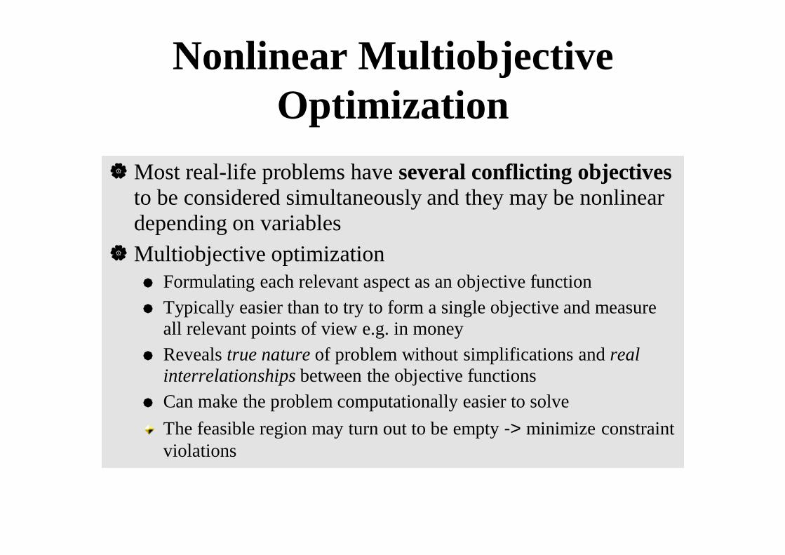
|Most real-life problems have several conflicting objectivesto be considered simultaneously and they may be nonlineardepending on variables

|Multiobjective optimizationÅ Formulating each relevant aspect as an objective functionÅ Typically easier than to try to form a single objective and measure

all relevant points of view e.g. in moneyÅ Reveals true nature of problem without simplifications and real

interrelationships between the objective functionsÅ Can make the problem computationally easier to solve

The feasible region may turn out to be empty -> minimize constraintviolations

Problem

fi: S®R = objective functionk (³ 2) = number of

(conflicting) objectivefunctions

x = decision vector (of ndecision variables xi)

S Ì Rn = feasible regionformed by constraintfunctions and

``minimize´´ = minimize theobjective functionssimultaneously

some constraint/objectivefunctions is nonlinear

We consider multiobjective optimization problems

where

Concepts| S consists of linear, nonlinear and/or box

constraints for the variables|We denote objective function values by zi = fi(x)| z = (z1,…, zk) is an objective vector| Z Ì Rk denotes the image of S; feasible

objective regionThus z Î Z

Definition: If all functions are linear, problem islinear (MOLP). If some functions are nonlinear,we have a nonlinear multiobjective optimizationproblem. Problem is nondifferentiable if somefunctions are nondifferentiable and convex if allobjectives and S are convex

Optimality|Contradiction and possible incommensurability Þ|x*Î S is Pareto optimal (PO) if there does not exist

another xÎS such that fi(x) £ fi(x*) for all i=1,…,k andfj(x) < fj(x*) for at least one j. Objective vector z*=f(x*)ÎZ is Pareto optimal if x* isi.e. (z* - Rk

+\{0}) Ç Z = Æ,that is, (z* - Rk

+) Ç Z = z*.|PO solutions form a (possibly

nonconvex and disconnected) PO set|x*Î S is weakly PO if there does not exist another xÎ S

such that fi(x) < fi(x*) for all i=1,…,ki.e. (z* - int Rk

+) Ç Z = Æ.|Properly PO: unbounded trade-offs are

not allowed. Weak PO É PO É proper PO

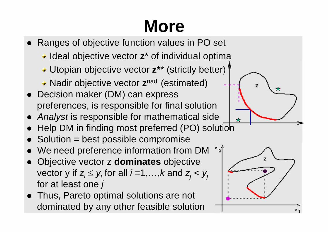
Morel Ranges of objective function values in PO set

Ideal objective vector z* of individual optimaUtopian objective vector z** (strictly better)Nadir objective vector znad (estimated)

l Decision maker (DM) can expresspreferences, is responsible for final solution

l Analyst is responsible for mathematical sidel Help DM in finding most preferred (PO) solutionl Solution = best possible compromisel We need preference information from DMl Objective vector z dominates objective

vector y if zi £ yi for all i =1,…,k and zj < yjfor at least one j

l Thus, Pareto optimal solutions are notdominated by any other feasible solution

Local and Global Optimality| Paying attention to the Pareto optimal set and

forgetting other solutions is acceptable only ifwe know that no unexpressed orapproximated objective functions areinvolved!

| Assuming DM is rational and problemcorrectly specified, final solution is always PO

| A point x*Î S is locally Pareto optimal if it isPareto optimal in some environment of x*

| Global Pareto optimality Þ local Paretooptimality

| Local PO Þ global PO, if S convex, fi:squasiconvex with at least one strictlyquasiconvex fi

More Concepts|Value function U:Rk®R may represent preferences|If U(z1) > U(z2) then the DM prefers z1 to z2. If U(z1)

= U(z2) then z1 and z2 are equally good (indifferent)|U is assumed to be strongly decreasing = less is

preferred to more. Implicit U is often assumed

|Decision making can be thought of being based oneither value maximization or satisficing

|An objective vector containing the aspiration levels žiof the DM is called a reference point žÎRk

Results|Sawaragi, Nakayama, Tanino: Pareto

optimal solution(s) exist ifÅ the objective functions are lower

semicontinuous andÅ the feasible region is nonempty and

compact|Karush-Kuhn-Tucker optimality

conditions can be formed as a naturalextension to single objectiveoptimization for both differentiable andnondifferentiable problems

Trading off|Moving from one PO solution to another = trading off|Definition: Given x1 and x2 Î S, the ratio of change

between fi and fj is

|Lij is a partial trade-off if fl(x1) = fl(x2) for all l=1,…,k,l ¹i,j. If fl(x1) ¹ fl(x2) for at least one l and l ¹ i,j, thenLij is a total trade-off

|Let d* be a feasible direction from x* Î S. The totaltrade-off rate along the direction d* is

|If fl(x*+ad*) = fl(x*) " l ¹i,j and for all 0 £a£a*, then lijis a partial trade-off rate

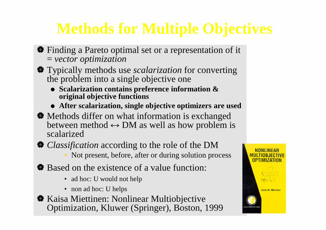
Methods for Multiple Objectives| Finding a Pareto optimal set or a representation of it

= vector optimization| Typically methods use scalarization for converting

the problem into a single objective oneÅ Scalarization contains preference information &

original objective functionsÅ After scalarization, single objective optimizers are used

|Methods differ on what information is exchangedbetween method ↔ DM as well as how problem isscalarized

| Classification according to the role of the DM• Not present, before, after or during solution process

| Based on the existence of a value function:• ad hoc: U would not help• non ad hoc: U helps

| Kaisa Miettinen: Nonlinear MultiobjectiveOptimization, Kluwer (Springer), Boston, 1999

Scalarizing Functions

|Scalarization = combine preferences and originalproblem Þ scalarized single objectivesubproblem|Resulting subproblem is solved with an

appropriate single objective optimization method|Objective function is called scalarizing (or

scalarization) function|Desirable properties

ÅOptimal solution is POÅAny PO solution can be found

Criteria for Good DecisionSupport System

|Recognizes and generates PO solutions|Helps DM feel convinced that final solution

is the most preferred one or at least closeenough to that

|Helps DM to get a “holistic” view over POset

|Does not require too much time from DM tofind final solution

|Communication between DM and systemnot too complicated

|Provides reliable information aboutalternatives available

Four Classes of Methods| How to support DM?| Four types of methods (Hwang and Masud, 1979)| No decision maker – some neutral compromise solution| A priori methods: DM sets hopes and closest solution is found

Å Expectations may be too optimistic or pessimisticÅ Hard to express preferences without knowing the problem well

| A posteriori methods: generate representation of PO set+ Gives information about variety of PO solutionsÅ Expensive, computationally demandingÅ Difficult to represent the PO set if k > 2o Example: evolutionary multiobjective optimization methods

| Interactive methods: iterative search process+ Avoid difficulties above+ Solution pattern is formed and repeated iteratively+ Move around Pareto optimal set+ What can we expect DMs to be able to say?+ Goal: easiness of use+ Cognitively valid approaches: classification and

reference point consisting of aspiration levels| Further information: Kaisa Miettinen: Nonlinear Multiobjective

Optimization, Kluwer (Springer), 1999

Methods cont.|No-preference methods

Å Meth. of Global Criterion|A posteriori methods

Å Weighting MethodÅ e-Constraint MethodÅ Hybrid MethodÅ Method of Weig. MetricsÅ Achievement Scalarizing

Function Approach|A priori methods

Å Value Function MethodÅ Lexicographic OrderingÅ Goal Programming

|Interactive methodsÅ Interactive Surrogate Worth

Trade-Off MethodÅ GDF MethodÅ Tchebycheff MethodÅ Reference Point MethodÅ GUESS MethodÅ Reference Direction

ApproachÅ Satisficing Trade-Off

MethodÅ Light Beam SearchÅ NIMBUS Method

Tree Diagram of MethodsMiettinen (1999)

No-Preference Methods:Method of Global Criterion (Yu, Zeleny)

|Distance between z­ and Z is minimized byLp-metric:if global idealobjective vectoris known

| or by L¥-metric:

|Differentiable form of the latter:

Method of Global Criterion cont.

? The choice of paffects greatly thesolution

+ Solution of the Lp-metric (p < ¥) is PO

» Solution of the L¥-metric is weakly POand the problem hasat least one POsolution

+ Simple method (nospecial hopes areset)

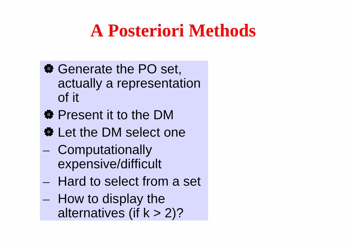
A Posteriori Methods

| Generate the PO set,actually a representationof it

| Present it to the DM| Let the DM select one– Computationally

expensive/difficult– Hard to select from a set– How to display the

alternatives (if k > 2)?

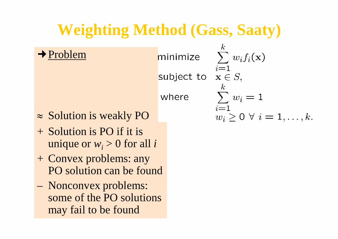
Weighting Method (Gass, Saaty)¢Problem

» Solution is weakly PO+ Solution is PO if it is

unique or wi > 0 for all i+ Convex problems: any

PO solution can be found– Nonconvex problems:

some of the PO solutionsmay fail to be found

Weighting Method cont.

– Weights are not easy to be understood(correlation, nonlinear affects). Small change inweights may change the solution dramatically

– Evenly distributed weights do not produce anevenly distributed representation of the PO set

e-Constraint Method (Haimes et al)

| Problem

» The solution is weakly Pareto optimal+ x* is PO iff it is a solution when ej = fj(x*)

(i=1,…,k, j¹l) for all objectives to be minimized+ A unique solution is PO+ Any PO solution can be found with some effort- There may be difficulties in specifying upper

bounds

Trade-Off Information

| Let the feasible region be of the formS = {x ÎRn | g(x) = (g1(x),…, gm(x)) T £ 0}

| Lagrange function of the e-constraintproblem is

| Under certain assumptions the coefficientslj= llj are (partial or total) trade-off rates

Method of Weighted Metrics (Zeleny)

| Weighted metric formulations are

Method of Weighted Metrics cont.+ If the solution is unique or the weights are positive,

the solution of Lp-metric (p<¥) is PO+ For positive weights, the solution of L¥-metric is

weakly PO and there exists at least one PO solution+ Any PO solution can be found with the L¥-metric

with positive weights if the reference point isutopian but some of the solutions may be weakly PO

- All the PO solutions may not be found with p<¥|

where r>0. This generates properly PO solutionsand any properly PO solution can be found

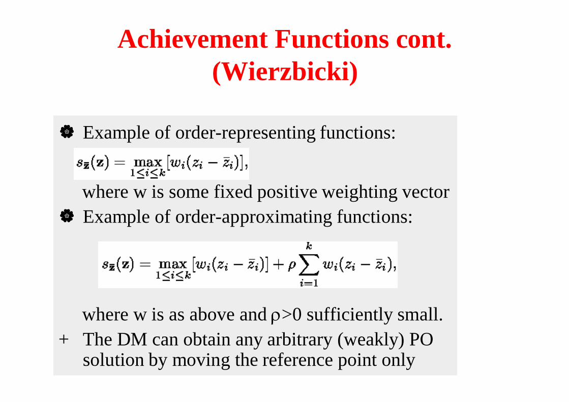
Achievement Functions cont.(Wierzbicki)

| Example of order-representing functions:

where w is some fixed positive weighting vector| Example of order-approximating functions:

where w is as above and r>0 sufficiently small.+ The DM can obtain any arbitrary (weakly) PO

solution by moving the reference point only

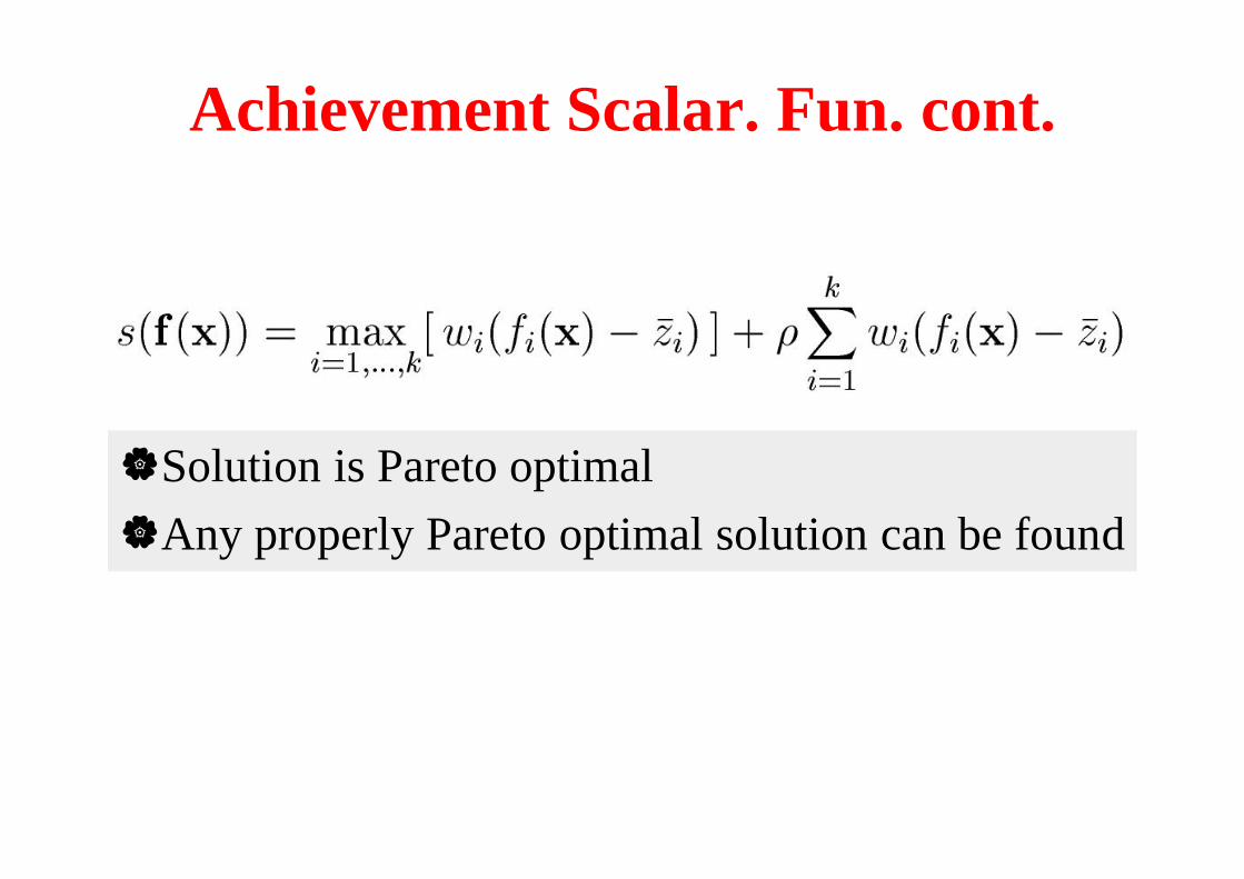
Achievement Scalar. Fun. cont.

|Solution is Pareto optimal|Any properly Pareto optimal solution can be found

Two Worlds: MCDM and EMO

Multiple criteria decisionmakingÅ Role of DM and decision

support emphasizedÅ Role of preference

information importantÅ Different types of methods -

interactive ones widelydeveloped

Å Solid theoretical background(we can prove Paretooptimality etc.)

Å Scalarization combiningobjective and preferences intoreal-valued functions

Evolutionary multiobjectiveoptimization (EMO)ÅIdea to approximate the set of Pareto

optimal solutionsÅCriteria: minimize distance to real

PO set and maximize diversity ofapproximation

ÅNot too much emphasis on DM’spreferences until recently

ÅCannot guarantee actual optimalityÅE.g. nonconvexity and discontinuity

cause no difficultiesÅBackground in applicationsÅMany benchmark problems for

testing goodness of methods (tomeasure quality of approximationgenerated) + performance criteria

ÅTerminology: bi-multi-manyÅNondominated = PO in a subset

EMOl Evolutionary algorithms: common metaheuristicsl Work well for mathematically difficult problems (no

assumptions)l Population-based approachesl Population of solutions is manipulated with

operations (selection, crossover, mutation) and thepopulation approximates the PO set

l Many different EMO methods existl Problems

– Diversity preserving mechanisms– Getting close to really PO solutions

l On the other hand– Computational effort is wasted in finding undesired solutions– Many solutions are presented to DM who can be unable to

compare and find most preferred among them when k > 2Many EMO methods do not work well when k>2 or 3Combine ideas of MCDM and EMO methods

EMO cont.| Population-based methods

Å Variables can be coded indifferent waysÅ Repeated for generationsÅ At every generation, generates a set of solutions

| VEGA, RWGA, MOGA, NSGA, NSGA-II,DPGA, SPEA-2 etc.Å Work best when k=2

| Goals: maintaining diversity and guaranteeingPareto optimality – how to measure?

| Special operators have been introduced| Typically tested with benchmark problems

with known PO sets| For k>3: MOEA/D, NSGA-III, RVEA etc.

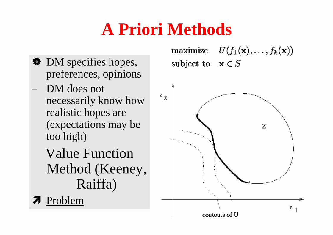
A Priori Methods

| DM specifies hopes,preferences, opinions

- DM does notnecessarily know howrealistic hopes are(expectations may betoo high)Value FunctionMethod (Keeney,

Raiffa)ì Problem

Lexicographic Ordering|The DM must specify an absolute order of

importance for objectives, i.e., fi >>> fi+1>>> ….|If the most important objective has a unique

solution, stop. Otherwise, optimize the second mostimportant objective such that the most importantobjective maintains its optimal value etc.

+ The solution is Pareto optimal.+ Some people make decisions successively.- Difficulty: specify the absolute order of importance.- The method is robust. The less important objectives

have very little chances to affect the final solution- Trading off is impossible

Interactive Methods|Most developed class of methods| A solution pattern is formed and repeated iteratively| DM directs the solution process, i.e. movement around PO set| DM needs time and interest for co-operation| Only some PO points (those that are interesting to the DM)

are generated| DM is not overloaded with information| DM can learn: specify and correct preferences and selections

as the solution process continues| DM has more confidence in the final solution| Important aspects

Å what is asked – what can we expect DMs to be able to say?Å what is told – goal: easiness of useÅ how the problem is scalarized

| Psychological convergence!

Interactive Methods, cont.

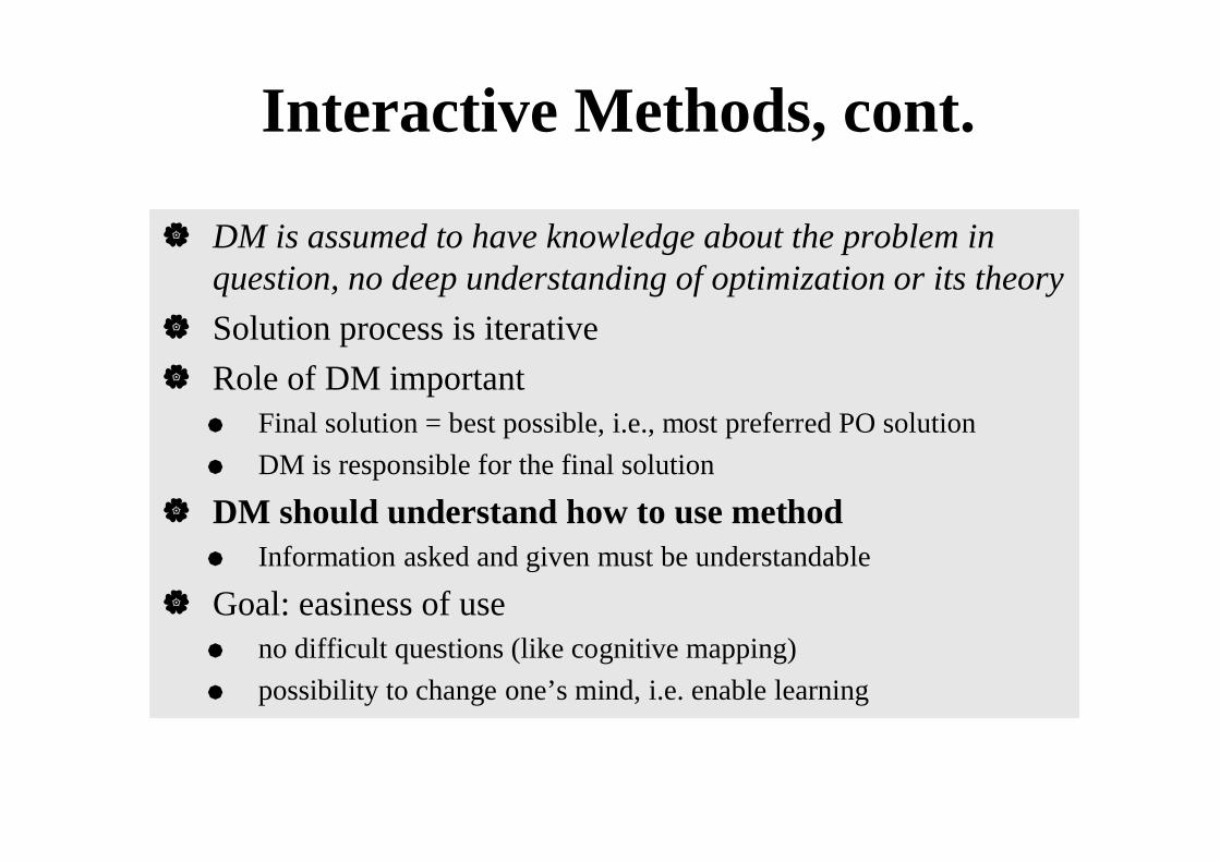
| DM is assumed to have knowledge about the problem inquestion, no deep understanding of optimization or its theory

| Solution process is iterative| Role of DM important

Å Final solution = best possible, i.e., most preferred PO solutionÅ DM is responsible for the final solution

| DM should understand how to use methodÅ Information asked and given must be understandable

| Goal: easiness of useÅ no difficult questions (like cognitive mapping)Å possibility to change one’s mind, i.e. enable learning

Interactive Methods, cont.

ØIn each iteration, the DM is shown Pareto optimalsolutions and asked to specify new preferenceinformation to generate more satisfactory newPareto optimal solution(s)ØThus, DM influences from which part of the Pareto

optimal set solutions are consideredØDM obtains

Ø new information and insight about the interdependenciesamong objective functions

Ø understanding of the feasibility of preferencesØNew knowledge obtained may affect preferences,

leading to solutions which were not previouslyconsideredØUser interface plays an important role

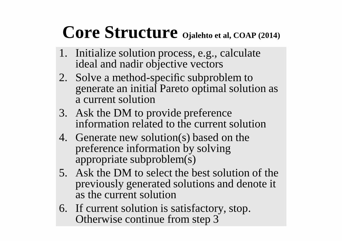
Core Structure Ojalehto et al, COAP (2014)

1. Initialize solution process, e.g., calculateideal and nadir objective vectors

2. Solve a method-specific subproblem togenerate an initial Pareto optimal solution asa current solution

3. Ask the DM to provide preferenceinformation related to the current solution

4. Generate new solution(s) based on thepreference information by solvingappropriate subproblem(s)

5. Ask the DM to select the best solution of thepreviously generated solutions and denote itas the current solution

6. If current solution is satisfactory, stop.Otherwise continue from step 3

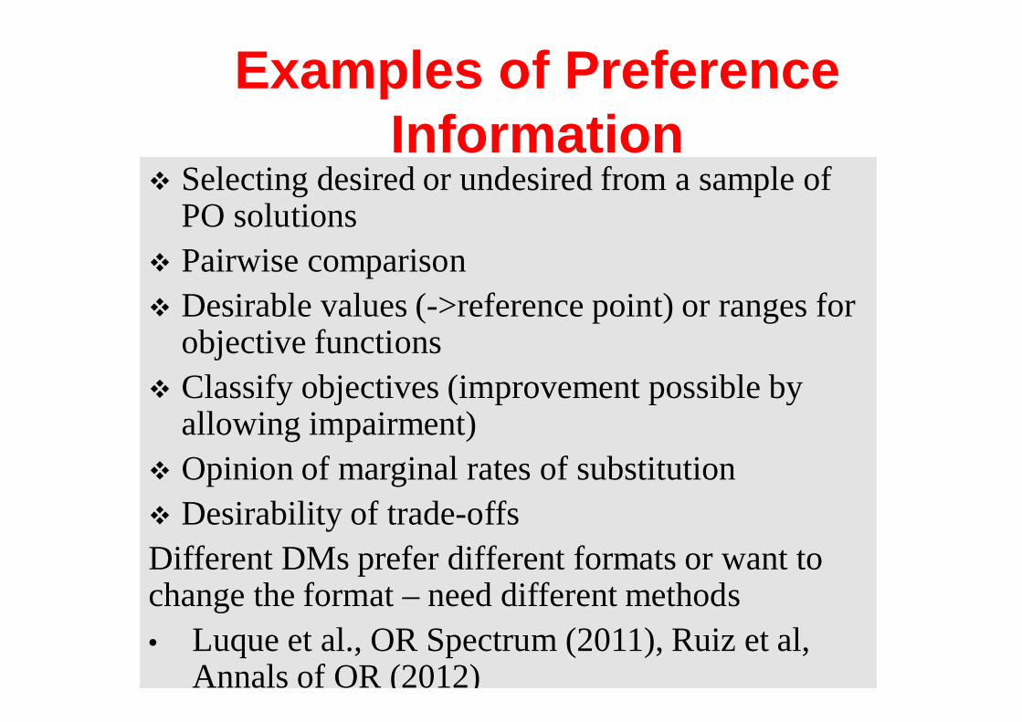
Examples of PreferenceInformation

v Selecting desired or undesired from a sample ofPO solutions

v Pairwise comparisonv Desirable values (->reference point) or ranges for

objective functionsv Classify objectives (improvement possible by

allowing impairment)v Opinion of marginal rates of substitutionv Desirability of trade-offsDifferent DMs prefer different formats or want tochange the format – need different methods• Luque et al., OR Spectrum (2011), Ruiz et al,

Annals of OR (2012)

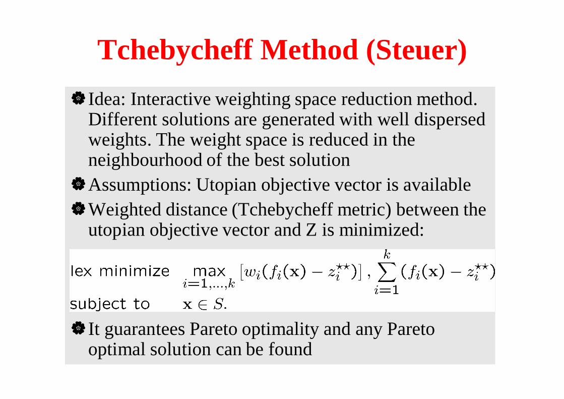
Tchebycheff Method (Steuer)|Idea: Interactive weighting space reduction method.

Different solutions are generated with well dispersedweights. The weight space is reduced in theneighbourhood of the best solution

|Assumptions: Utopian objective vector is available|Weighted distance (Tchebycheff metric) between the

utopian objective vector and Z is minimized:

|It guarantees Pareto optimality and any Paretooptimal solution can be found

Tchebycheff Method cont.|At first, weights between [0,1] are generated.|Iteratively, the upper and lower bounds of the

weighting space are tightened.|Algorithm1) Specify number of alternatives P and number of

iterations H. Construct z­­. Set h=1.2) Form the current weighting vector space and

generate 2P dispersed weighting vectors.3) Solve the problem for each of the 2P weights.4) Present the P most different of the objective

vectors and let the DM choose the most preferred.5) If h=H, stop. Otherwise, gather information for

reducing the weight space, set h=h+1 and go to 2).

Tchebycheff Method cont.|Non ad hoc method+ All the DM has to do is to compare several Pareto

optimal objective vectors and select the mostpreferred one.

! The ease of the comparison depends on P and k.- The discarded parts of the weighting vector space

cannot be restored if the DM changes her/his mind.- A great deal of calculation is needed at each

iteration and many of the results are discarded.

+ Parallel computing can be utilized.

Reference Point Method (Wierzbicki)| Idea: Direct the search by reference points

representing desirable values for theobjectives and generate new alternatives byshifting the reference point

| Reference point is projected onto PO set withachievement scalarizing function

| Solution is properly PO

Reference Point Method Algorithm

| No specific assumptions| Algorithm:1) Present information to the DM. Set h=1.2) Ask the DM to specify a reference point žh.3) Minimize ach. function. Present zh to the DM.4) Calculate k other solutions with reference points

where dh=||žh - zh|| and ei is the ith unit vector.5) If the DM can select the final solution, stop.

Otherwise, ask the DM to specify žh+1. Set h=h+1and go to 3).

Reference Point Method cont.

|Ad hoc method (or both)+ Easy for the DM to understand: (s)he has to

specify aspiration levels and compare objectivevectors.

+ For nondifferentiable problems, as well+ No consistency required- Easiness of comparison depends on the problem- No clear strategy to produce the final solution

Satisficing Trade-Off Method(Nakayama et al)

| Idea: To classify the objective functions:Å functions to be improvedÅ acceptable functionsÅ functions whose values can be relaxed

|AssumptionsÅ functions are twice continuously differentiableÅ trade-off information is available in the KKT multipliers

|Aspiration levels from the DM, upper bounds from theKKT multipliers

| Satisficing decision making is emphasized

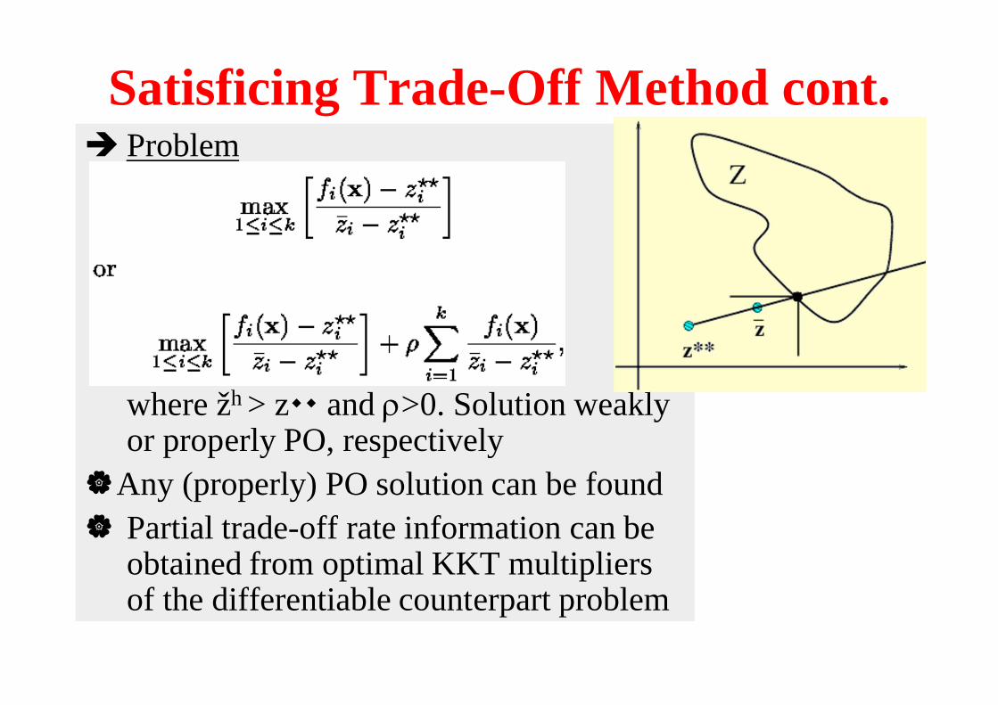
Satisficing Trade-Off Method cont.è Problem

where žh > z­­ and r>0. Solution weaklyor properly PO, respectively

|Any (properly) PO solution can be found| Partial trade-off rate information can be

obtained from optimal KKT multipliersof the differentiable counterpart problem

Satisficing Trade-Off Algorithm

1) Calculate z­­ and get a starting solution.2) Ask the DM to classify the objective functions

into the three classes. If no improvements aredesired, stop.

3) If trade-off rates are not available, ask the DM tospecify aspiration levels and upper bounds.Otherwise, ask the DM to specify aspirationlevels. Utilize automatic trade-off in specifyingthe upper bounds for the functions to be relaxed.Let the DM modify the calculated levels, ifnecessary.

4) Solve the problem. Go to 2).

Background for NIMBUSÒ

| DM should understand how to use method| Solution = best possible compromise| DM is responsible for the final solution| Difficult to present the Pareto optimal set,

expectations may be too high| Interactive approach avoids these difficulties| Move around Pareto optimal set| How can we support the learning process?| DM should be able to direct the solution process| Goal: easiness of use Þ no difficult questions &

possibility to change one’s mind| Dealing with objective function values is

understandable and straightforward

Synchronous NIMBUSÒ

Miettinen, Mäkelä, EJOR (2006)l Scalarization is important: contains preference informationl But scalarizations based on same input give different

solutions (Miettinen, Mäkelä, OR Spec (2002))l Which is the best? Þ Synchronous NIMBUSÒ

l 1-4 scalarized problem(s) formed to obtain different POsolutions

l Show them to the DM & let her/him choose the bestl DM can see how realistic hopes were and can adjust theml Versatile possibilities to direct solution process

l Besides classification, intermediate solutions betweenPO solutions can be generated

l Classification and comparison of alternatives are used inthe extent the DM desires

l DM can learn during the iterative solution process and onlyPO solutions that are interesting to her/him are generated

Classification in NIMBUS

| DM directs the search by classification: Classification ofobjective functions into up to 5 classes

| Classification: DM indicates desirable changes in thecurrent PO objective function values fi(xh)

| Classes: functions fi whose valuesÅ should be decreased (iÎI<)Å should be decreased till some aspiration level ži

h < fi(xh) (iÎI£)Å are satisfactory at the moment (iÎI=)Å are allowed to increase up till some upper bound ei

h>fi(xh) (iÎI>)Å are allowed to change freely (iÎIà)

| DM must be willing to give up something| Miettinen, Mäkelä: Optim (1995), JORS (1999), Comp&OR

(2000), EJOR (2006)

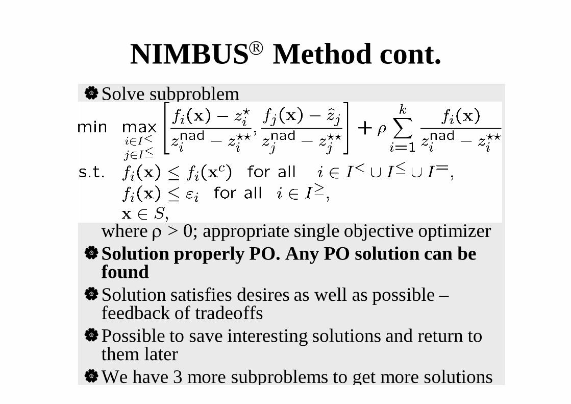
NIMBUSÒ Method cont.|Solve subproblem

where r > 0; appropriate single objective optimizer|Solution properly PO. Any PO solution can be

found|Solution satisfies desires as well as possible –

feedback of tradeoffs|Possible to save interesting solutions and return to

them later|We have 3 more subproblems to get more solutions

Other Subproblems

|Classification implies reference point but not viceversa

|We use reference point based subproblems|Components of reference point are obtained from

classification informationÅ I< : corresponding component of ideal objective vectorÅ I£ : aspiration level specified by the DMÅ I = : current objective function valuerÅ I³ : upper bound specified by the DMÅ I> : corresponding component of nadir objective vector

| Intermediate solutions between xh and x’h: f(xh+tjdh), where dh=xh’- xh and tj=j/(P+1)

| Search iteratively around the PO set until DM does not want toimprove or impair any objective

| Ad hoc method+ Versatile possibilities for the DM: classification, comparison,

extracting undesirable solutions+ Does not depend entirely on how well the DM manages in

classification. (S)he can e.g. specify loose upper bounds andget intermediate solutions

+ Works for nondifferentiable/nonconvex problems+ No consistency is required – learning-oriented method

NIMBUS Method - Remarks

1) Choose starting solution and project it to be PO.2) Ask DM to classify the objectives and to specify

related parameters. Solve 1-4 subproblems.3) Present different solutions to DM.4) If DM wants to save solutions, update database.5) If DM does not want to see intermediate solutions,

go to 7). Otherwise, ask DM to select the end pointsand the number of solutions.

6) Generate and project intermediate solutions. Go to3).

7) Ask DM to choose the most preferred solution. IfDM wants to continue, go to 2). Otherwise, stop.

NIMBUSÒ Algorithm

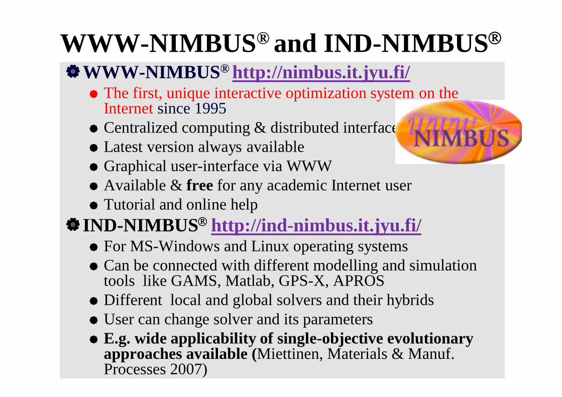
|WWW-NIMBUS® http://nimbus.it.jyu.fi/Å The first, unique interactive optimization system on the

Internet since 1995Å Centralized computing & distributed interfaceÅ Latest version always availableÅ Graphical user-interface via WWWÅ Available & free for any academic Internet userÅ Tutorial and online help

|IND-NIMBUSÒ http://ind-nimbus.it.jyu.fi/Å For MS-Windows and Linux operating systemsÅ Can be connected with different modelling and simulation

tools like GAMS, Matlab, GPS-X, APROSÅ Different local and global solvers and their hybridsÅ User can change solver and its parametersÅ E.g. wide applicability of single-objective evolutionary

approaches available (Miettinen, Materials & Manuf.Processes 2007)

WWW-NIMBUS® and IND-NIMBUSÒ

IND-NIMBUSÒ ViewsObjectivefunctionvalues andclassification

Numericalclassificationboundaries

Initial POsolution

IND-NIMBUSÒ Views

NIMBUSclassificationby clickingobjective bar

Newsolutionscalculatedwith a playbutton

New POsolutions

Initial POsolution

Computational Challenges

of complex simulation-based optimizationWe need tools for handlingl Computational cost

– Objective and constraint functions depend on output ofsimulation models – may be time-consuming

l Black-box models– Global optimization needed -> computational cost

l One can train a computationally inexpensivesurrogate (metamodel) to each expensive functionbut training is not straightforward and there arealternatives

l EMO methods for computationally expensive:l ParEGO, SMS-EGO, K-RVEA

Hybrid Methodsl Put together ideas of different methods to form new

onesl Aim: at the same time

l combine strengths and benefitsl avoid weaknesses

l A posteriori methodsl information of whole PO set – possibilities and limitations

l Interactive methodsl DM can learn about the problem, its interdependencies

and adjust preferencesl DM can concentrate on interesting solutionsl computationally less costly

l Hybrids combining a posteriori and interactive methods

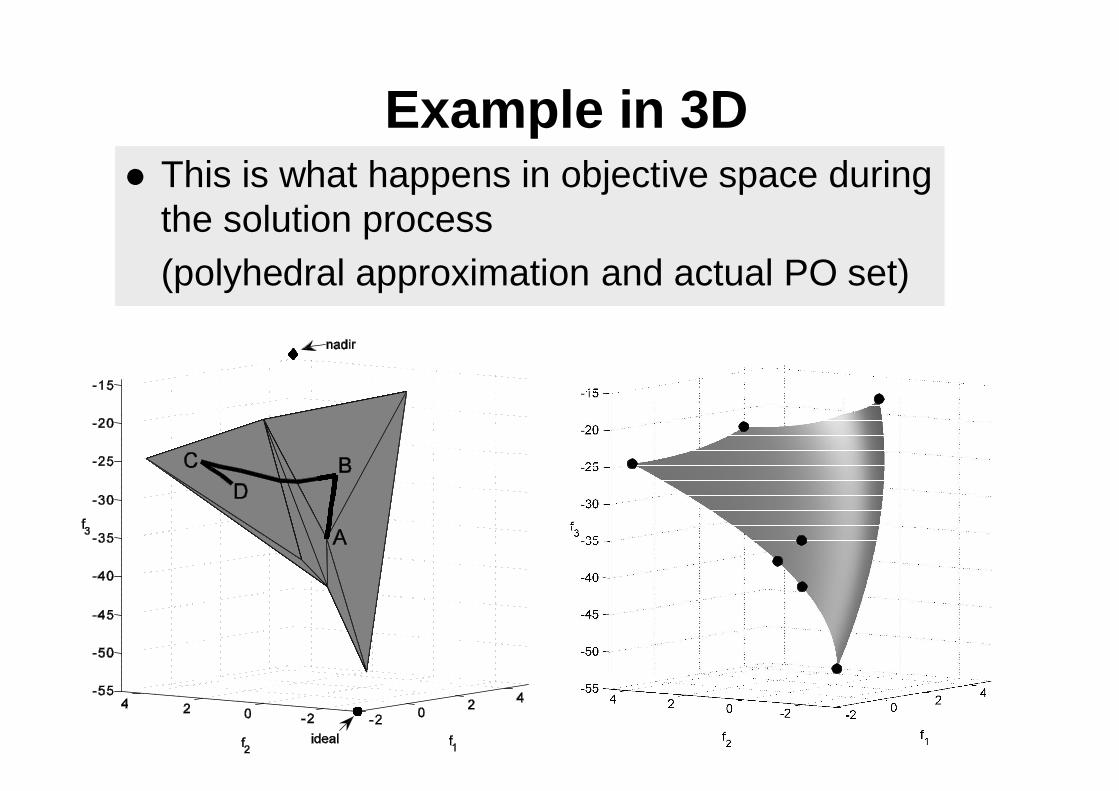
Pareto NavigatorEskelinen et al., OR Spectrum (2010)

l Background & motivation– I Learning phase II Decision phase– Challenges of computationally expensive problems

l Pareto optimal set = actual PO setl Learning-oriented interactive methodl Hybrid method: first a posteriori and then

interactive method (assume convexity)l relatively small) set of Pareto optimal solutionsl polyhedral approximation of PO set in objective

space – approximated PO setl Convenient and real-time navigation

– Preference information: reference point– Project to actual PO set

l Instead of approximating objective functionswe directly approximate PO set

Pareto Navigator ViewBased on theinformationgiven, newapproximatedPO solutionsare generated

to projectthem to realPO solutions

or as astarting pointfor newnavigation

Approximatedsolutions canbe used

l This is what happens in objective space duringthe solution process(polyhedral approximation and actual PO set)

Example in 3D

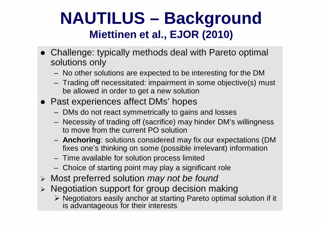
NAUTILUS – BackgroundMiettinen et al., EJOR (2010)

l Challenge: typically methods deal with Pareto optimalsolutions only– No other solutions are expected to be interesting for the DM– Trading off necessitated: impairment in some objective(s) must

be allowed in order to get a new solutionl Past experiences affect DMs’ hopes

– DMs do not react symmetrically to gains and losses– Necessity of trading off (sacrifice) may hinder DM’s willingness

to move from the current PO solution– Anchoring: solutions considered may fix our expectations (DM

fixes one’s thinking on some (possible irrelevant) information– Time available for solution process limited– Choice of starting point may play a significant role

Ø Most preferred solution may not be foundØ Negotiation support for group decision making

Ø Negotiators easily anchor at starting Pareto optimal solution if itis advantageous for their interests

Idea of NAUTILUS

l DM starts from the worst e.g. nadir objective vectorand moves towards PO setl Improvement in each objective at every iterationl Possible to gain at every iteration – no need for sacrifices

l At each iteration, objective vector obtaineddominates the previous one

l Only the final solution is Pareto optimall DM can always go backwards if desiredl DM can approach any part of PO set (s)he wishesl Different NAUTILUS variants use different ways of

expressing preference information to form directionof simultaneous improvementl Ruiz et al, EJOR (2015)l Miettinen et al, JOGO (2015)l Miettinen, Ruiz, J Bus Econ (2016)

1f

nadzz =0

lo,1zz =**

Z=f (S)

lo,2z

1f

1z2z

2f

lo,3z

At each iteration range of reachable obj. function values shrinks

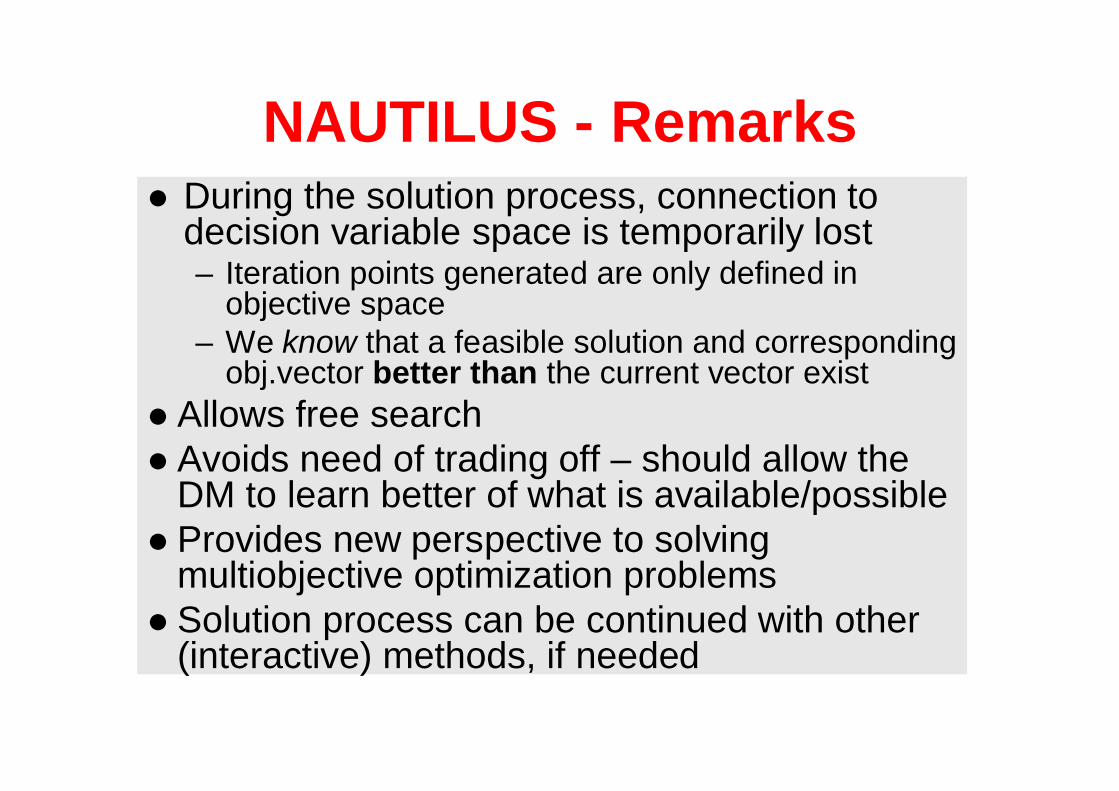
NAUTILUS - Remarksl During the solution process, connection to

decision variable space is temporarily lost– Iteration points generated are only defined in

objective space– We know that a feasible solution and corresponding

obj.vector better than the current vector existl Allows free searchl Avoids need of trading off – should allow the

DM to learn better of what is available/possiblel Provides new perspective to solving

multiobjective optimization problemsl Solution process can be continued with other

(interactive) methods, if needed

3-Stage ApproachSteponavice et al., Computer-Aided Design

(2014)

E-NAUTILUSRuiz et al., EJOR

(2015)

DM sets number of pointsto compare (here 6) andnumber of iterations (here 3)

NAUTILUS Navigatorwith A. B. Ruiz, F. Ruiz, V. Ojalehto

l Idea: DM can navigate from worst possible to mostpreferred objective function values

l A priori: Set of (approximated) PO solutions– Generated before involving DM

l Interaction: With NAUTILUS Navigator DM can navigatefrom inferior solution to most preferred one by gaining inall objective functions simultaneously, at each iteration

l Preference information: reference point (aspiration levels)and bounds not to be exceeded

l As solution process approaches set of PO solutions,ranges of objective function values that are still reachablewithout trading-off shrink and DM sees this in real time

NAUTILUS Navigator cont.• GUI with reachable range paths consisting of two plot lines;

lowest and highest reachable values from current iteration• DM can see history, no need to remember it

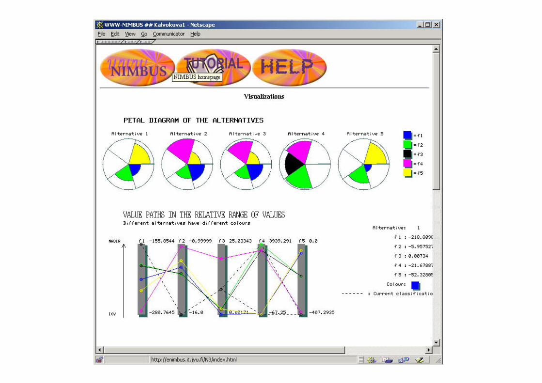
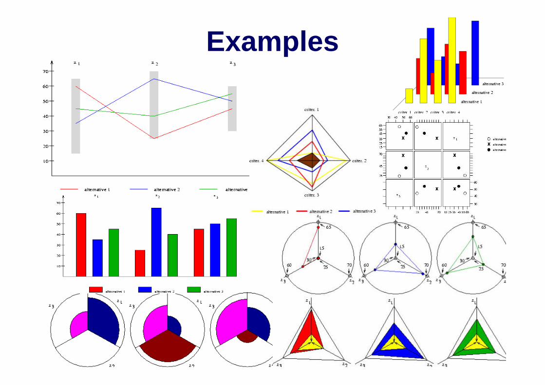
On Visual IllustrationMiettinen, OR Spec (2014)

l The decision maker (DM) is often asked tocompare several alternatives– e.g. within interactive methods– Graphs and table complement each other

l Illustration is difficult but important– easy to comprehend– important information should not be lost– no unintentional information should be included– makes it easier to see essential similarities and

differencesl DMs have different cognitive styles

Examples

Experiencesl Collaboration with experts of problem

domainsl Positive experiencesl DM receives a new perspective

– can consider different objectivessimultaneously, not one by one

– interdependencies and interactions betweenobjectives to be observed

– DM learns about the conflicting qualitativeproperties

– new insight to challenging and complexphenomena

l Experiences of DMs– methods easy to use – understandable

questions– DM can find a satisfactory solution and be

convinced of its goodness– confidence: best solution was found

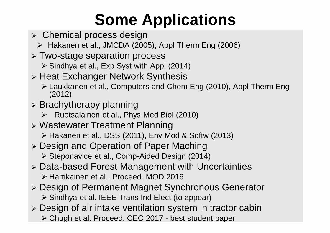
Some ApplicationsØ Chemical process designØ Hakanen et al., JMCDA (2005), Appl Therm Eng (2006)Ø Two-stage separation processØ Sindhya et al., Exp Syst with Appl (2014)

Ø Heat Exchanger Network SynthesisØ Laukkanen et al., Computers and Chem Eng (2010), Appl Therm Eng

(2012)Ø Brachytherapy planningØ Ruotsalainen et al., Phys Med Biol (2010)

Ø Wastewater Treatment PlanningØ Hakanen et al., DSS (2011), Env Mod & Softw (2013)

Ø Design and Operation of Paper MachingØ Steponavice et al., Comp-Aided Design (2014)

Ø Data-based Forest Management with UncertaintiesØ Hartikainen et al., Proceed. MOD 2016

Ø Design of Permanent Magnet Synchronous GeneratorØ Sindhya et al. IEEE Trans Ind Elect (to appear)

Ø Design of air intake ventilation system in tractor cabinØ Chugh et al. Proceed. CEC 2017 - best student paper

Furthermorel Open source framework DESDEO wit

interactive methods – try it!– desdeo.it.jyu.fi

l Decision analytics - data driven decisionsupport – thematic research area: DEMO– Instead of models we have data available– Applications incl. forest treatment planning,

inventory management and punishing criminals– http://www.jyu.fi/demo

l We welcome visitors!l Open PhD student positions twice a yearl EMO2019: www.emo2019.org/

Conclusionsl Compromise is better than optimum!l Plenty of real-life applications are waiting for

us and provide various challenges!l Hybridization of different methods offers a

lot of potentiall Book aims at bringing MCDM and EMO

fields closer to each other:Branke, Deb, Miettinen, Slowinski (Eds.):Multiobjective Optimization: Interactive andEvolutionary Approaches, Springer-Verlag, 2008

l Method selection depends e.g. on– Properties of problem– Availability of DM– Preference information type comfortable for DM

Acknowledgements®Collaboration: coauthors and

Industrial Optimization Grouphttp://www.mit.jyu.fi/optgroup/

®Funding: Partly Academy ofFinland, Tekes: Finnish FundingAgency for Innovation & companies