This document contains a post-print version of the paper Nonlinear pressure control of self-supplied variable displacement axial piston pumps authored by W. Kemmetmüller, F. Fuchshumer, and A. Kugi and published in Control Engineering Practice. The content of this post-print version is identical to the published paper but without the publisher’s final layout or copy editing. Please, scroll down for the article. Cite this article as: W. Kemmetmüller, F. Fuchshumer, and A. Kugi, “Nonlinear pressure control of self-supplied variable displacement axial piston pumps”, Control Engineering Practice, vol. 18, pp. 84–93, 2010. doi: 10.1016/j.conengprac.2009.09. 006 BibTex entry: % This file was created with JabRef 2.9.2. % Encoding: Cp1252 @ARTICLE{acinpaper, author = {Kemmetmüller, W. and Fuchshumer, F. and Kugi, A.}, title = {Nonlinear pressure control of self-supplied variable displacement axial piston pumps}, journal = {Control Engineering Practice}, year = {2010}, volume = {18}, pages = {84-93}, doi = {10.1016/j.conengprac.2009.09.006}, url = {http://www.sciencedirect.com/science/article/pii/S0967066109001701} } Link to original paper: http://dx.doi.org/10.1016/j.conengprac.2009.09.006 http://www.sciencedirect.com/science/article/pii/S0967066109001701 Read more ACIN papers or get this document: http://www.acin.tuwien.ac.at/literature Contact: Automation and Control Institute (ACIN) Internet: www.acin.tuwien.ac.at Vienna University of Technology E-mail: [email protected]Gusshausstrasse 27-29/E376 Phone: +43 1 58801 37601 1040 Vienna, Austria Fax: +43 1 58801 37699
Transcript
This document contains a post-print version of the paper
Nonlinear pressure control of self-supplied variable displacement axialpiston pumps
authored by W. Kemmetmüller, F. Fuchshumer, and A. Kugi
and published in Control Engineering Practice.
The content of this post-print version is identical to the published paper but without the publisher’s final layout orcopy editing. Please, scroll down for the article.
Cite this article as:W. Kemmetmüller, F. Fuchshumer, and A. Kugi, “Nonlinear pressure control of self-supplied variable displacementaxial piston pumps”, Control Engineering Practice, vol. 18, pp. 84–93, 2010. doi: 10.1016/j.conengprac.2009.09.006
BibTex entry:% This file was created with JabRef 2.9.2.% Encoding: Cp1252
@ARTICLE{acinpaper,author = {Kemmetmüller, W. and Fuchshumer, F. and Kugi, A.},title = {Nonlinear pressure control of self-supplied variable displacement
Link to original paper:http://dx.doi.org/10.1016/j.conengprac.2009.09.006http://www.sciencedirect.com/science/article/pii/S0967066109001701
Read more ACIN papers or get this document:http://www.acin.tuwien.ac.at/literature
Contact:Automation and Control Institute (ACIN) Internet: www.acin.tuwien.ac.atVienna University of Technology E-mail: [email protected] 27-29/E376 Phone: +43 1 58801 376011040 Vienna, Austria Fax: +43 1 58801 37699
Copyright notice:This is the authors’ version of a work that was accepted for publication in Control Engineering Practice. Changes resulting from thepublishing process, such as peer review, editing, corrections, structural formatting, and other quality control mechanisms may not bereflected in this document. Changes may have been made to this work since it was submitted for publication. A definitive versionwas subsequently published in W. Kemmetmüller, F. Fuchshumer, and A. Kugi, “Nonlinear pressure control of self-supplied variabledisplacement axial piston pumps”, Control Engineering Practice, vol. 18, pp. 84–93, 2010. doi: 10.1016/j.conengprac.2009.09.006
Nonlinear pressure control of self-supplied variable displacement axial piston pumps
W. Kemmetmuller∗,a, F. Fuchshumerb, A. Kugia
aAutomation and Control Institute, Vienna University of Technology, Gusshausstr. 27–29, 1040 Vienna, AustriabHydac Electronic GmbH, Hauptstr. 27, 66128 Saarbrucken, Germany
Abstract
The present paper deals with the pressure control of self-supplied variable displacement axial piston pumps subject to fast changing,
unknown loads. First, the setup of the system and the mathematical model are described. As the pump is self-supplied, the
mathematical model exhibits a switching right-hand side which makes the control design a challenging task. A nonlinear two
degrees-of-freedom control strategy, comprising a feedforward and a feedback control, in combination with a load estimator is
proposed for the pressure control. The proof of the stability of the overall closed-loop system is based on Lyapunov’s theory. The
performance of the control concept is verified by means of experiments. The results show that the proposed control concept has an
Since electrohydraulic systems exhibit a significant nonlinear
behavior the performance of the closed-loop system is normally
rather limited. Furthermore, a rigorous stability proof is lacking
in most cases and the tuning of the controller parameters turns
out to be very time-consuming. In this work, a new model-
based nonlinear control strategy is derived, which, on the one
hand, takes into account the essential nonlinearities of the sys-
tem and, on the other hand, can be easily adjusted to pumps of
different installation sizes in the same model range.
A general problem in designing a load-sensing system is to
find out the actual demands of the load, since in most cases the
load is neither known nor can it be measured. This problem
also occurs in the application considered in this paper where
the load not only is unknown but may also change in a very
fast manner. In order to deal with this fact, the nonlinear con-
trol strategy has to be augmented by a load estimator. This is
a challenging task since it is well known that the separation
principle of the controller and the estimator design does not
hold for nonlinear systems. In this contribution, the stability of
the closed-loop system consisting of the nonlinear controller,
the nonlinear load estimator and the plant model is proven by
means of Lyapunov’s theory.
In order to meet the high demands both on the tracking
behavior and the robustness of the closed-loop system a two
degrees-of-freedom control structure, comprising a feedfor-
ward and a feedback part, is proposed in the controller design.
Thereby, the design of the control strategy becomes very chal-
Preprint submitted to Control Engineering Practice September 11, 2009
Post-print version of the article: W. Kemmetmüller, F. Fuchshumer, and A. Kugi, “Nonlinear pressure control of self-supplied variabledisplacement axial piston pumps”, Control Engineering Practice, vol. 18, pp. 84–93, 2010. doi: 10.1016/j.conengprac.2009.09.006The content of this post-print version is identical to the published paper but without the publisher’s final layout or copy editing.
& Ivantysynova M, 1993; Findeisen, 2006). Since the detailed
mathematical models capturing all the dynamical effects are in
general rather complicated they are not suitable for a model
2
Post-print version of the article: W. Kemmetmüller, F. Fuchshumer, and A. Kugi, “Nonlinear pressure control of self-supplied variabledisplacement axial piston pumps”, Control Engineering Practice, vol. 18, pp. 84–93, 2010. doi: 10.1016/j.conengprac.2009.09.006The content of this post-print version is identical to the published paper but without the publisher’s final layout or copy editing.
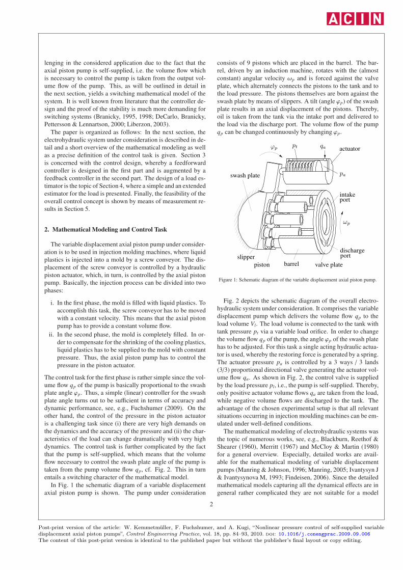
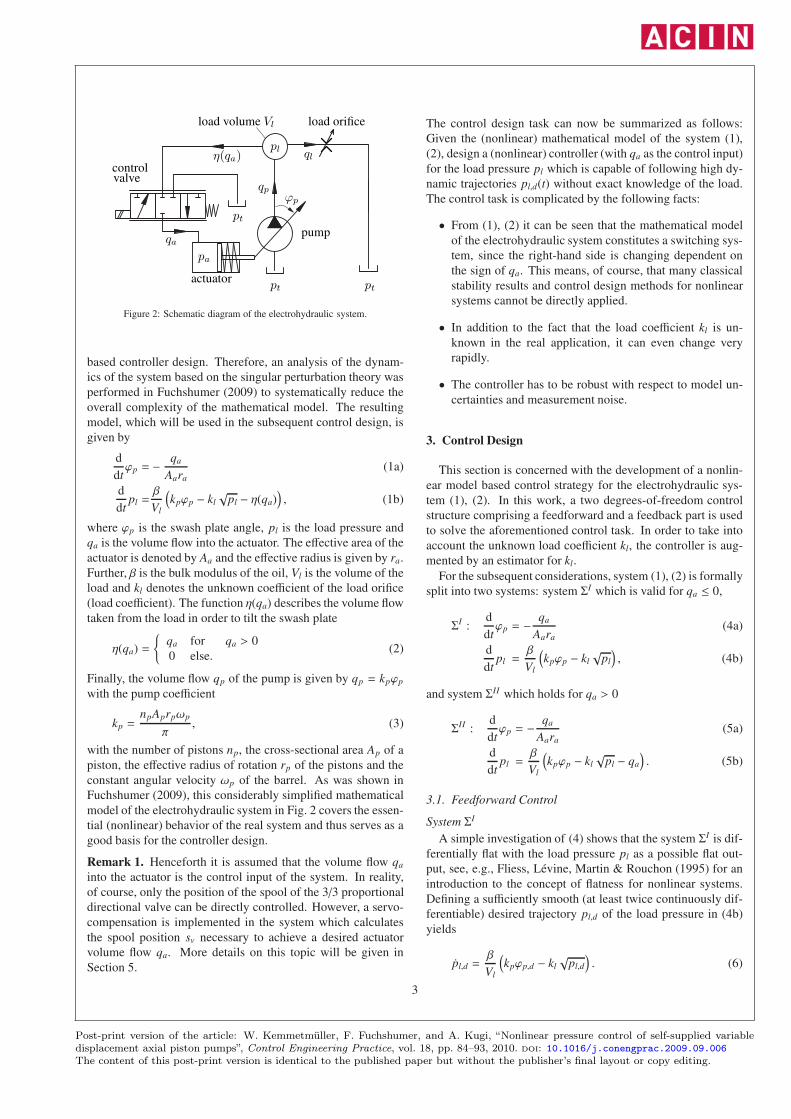
Figure 2: Schematic diagram of the electrohydraulic system.
based controller design. Therefore, an analysis of the dynam-
ics of the system based on the singular perturbation theory was
performed in Fuchshumer (2009) to systematically reduce the
overall complexity of the mathematical model. The resulting
model, which will be used in the subsequent control design, is
given by
d
dtϕp = − qa
Aara
(1a)
d
dtpl =β
Vl
(kpϕp − kl
√pl − η(qa)
), (1b)
where ϕp is the swash plate angle, pl is the load pressure and
qa is the volume flow into the actuator. The effective area of the
actuator is denoted by Aa and the effective radius is given by ra.
Further, β is the bulk modulus of the oil, Vl is the volume of the
load and kl denotes the unknown coefficient of the load orifice
(load coefficient). The function η(qa) describes the volume flow
taken from the load in order to tilt the swash plate
η(qa) =
{qa for qa > 0
0 else.(2)
Finally, the volume flow qp of the pump is given by qp = kpϕp
with the pump coefficient
kp =npAprpωp
π, (3)
with the number of pistons np, the cross-sectional area Ap of a
piston, the effective radius of rotation rp of the pistons and the
constant angular velocity ωp of the barrel. As was shown in
Fuchshumer (2009), this considerably simplified mathematical
model of the electrohydraulic system in Fig. 2 covers the essen-
tial (nonlinear) behavior of the real system and thus serves as a
good basis for the controller design.
Remark 1. Henceforth it is assumed that the volume flow qa
into the actuator is the control input of the system. In reality,
of course, only the position of the spool of the 3/3 proportional
directional valve can be directly controlled. However, a servo-
compensation is implemented in the system which calculates
the spool position sv necessary to achieve a desired actuator
volume flow qa. More details on this topic will be given in
Section 5.
The control design task can now be summarized as follows:
Given the (nonlinear) mathematical model of the system (1),
(2), design a (nonlinear) controller (with qa as the control input)
for the load pressure pl which is capable of following high dy-
namic trajectories pl,d(t) without exact knowledge of the load.
The control task is complicated by the following facts:
• From (1), (2) it can be seen that the mathematical model
of the electrohydraulic system constitutes a switching sys-
tem, since the right-hand side is changing dependent on
the sign of qa. This means, of course, that many classical
stability results and control design methods for nonlinear
systems cannot be directly applied.
• In addition to the fact that the load coefficient kl is un-
known in the real application, it can even change very
rapidly.
• The controller has to be robust with respect to model un-
certainties and measurement noise.
3. Control Design
This section is concerned with the development of a nonlin-
ear model based control strategy for the electrohydraulic sys-
tem (1), (2). In this work, a two degrees-of-freedom control
structure comprising a feedforward and a feedback part is used
to solve the aforementioned control task. In order to take into
account the unknown load coefficient kl, the controller is aug-
mented by an estimator for kl.
For the subsequent considerations, system (1), (2) is formally
split into two systems: system ΣI which is valid for qa ≤ 0,
ΣI :d
dtϕp = − qa
Aara
(4a)
d
dtpl =
β
Vl
(kpϕp − kl
√pl
), (4b)
and system ΣII which holds for qa > 0
ΣII :d
dtϕp = − qa
Aara
(5a)
d
dtpl =
β
Vl
(kpϕp − kl
√pl − qa
). (5b)
3.1. Feedforward Control
System ΣI
A simple investigation of (4) shows that the system ΣI is dif-
ferentially flat with the load pressure pl as a possible flat out-
put, see, e.g., Fliess, Levine, Martin & Rouchon (1995) for an
introduction to the concept of flatness for nonlinear systems.
Defining a sufficiently smooth (at least twice continuously dif-
ferentiable) desired trajectory pl,d of the load pressure in (4b)
yields
pl,d =β
Vl
(kpϕp,d − kl
√pl,d
). (6)
3
Post-print version of the article: W. Kemmetmüller, F. Fuchshumer, and A. Kugi, “Nonlinear pressure control of self-supplied variabledisplacement axial piston pumps”, Control Engineering Practice, vol. 18, pp. 84–93, 2010. doi: 10.1016/j.conengprac.2009.09.006The content of this post-print version is identical to the published paper but without the publisher’s final layout or copy editing.
2000; Liberzon, 2003). Therefore, it is not sufficient to design
a stabilizing controller for the error systems (13) and (14) sepa-
rately. One possibility to achieve a systematic proof of the sta-
bility of switched systems is given by the method of multiple
Lyapunov functions as proposed by Branicky (1998). Thereby,
the stability of each system has to be proven with a Lyapunov
function and in addition it has to be shown that each Lyapunov
function is strictly non-increasing during switching. While the
proof of the first condition is rather straightforward for many
systems, the proof of the second condition is in general diffi-
cult. One way to avoid the proof of the second condition is to
use a common Lyapunov function for all systems. Although
the design of a common Lyapunov function turns out to be a
rather delicate issue for general nonlinear switching systems,
this approach will be pursued in the following.
For the time being, it is assumed that a common Lyapunov
function and feedback controllers FBI and FBII for the error
systems I and II, respectively, have already been found such
that the stability of each closed-loop system is guaranteed2. At
this point the question arises when and how the control law con-
sisting of the feedforward and the feedback control is switched.
The intuitive approach would be that FF I + FBI are active for
qa ≤ 0 and FF II + FBII for qa > 0.
Then, however, two problems occur: First, switching the
feedforward control FF I and FF II based on qa = 0 yields to
discontinuities in the desired value of the swash plate angle ϕp,d
and thus in eϕ. In order to make this more obvious, consider at
the beginning that qa = qa,d + qa,c < 0 and therefore FF I and
FBI are active. If at time ts the volume flow qa equals zero,
switching to FF II and FBII would occur. In this case, the ini-
tial value ϕp,d(ts) of the differential equation (12) would be set
to the actual value of ϕp,d at t = ts in FF I due to (7) and thus
the trajectory is continuous. However, switching from qa > 0
(i.e. FF II and FBII are active) to FF I and FBI at time t = ts
when qa = 0, the desired swash plate angle ϕp,d has to satisfy
the following relations at t = ts
ϕp,d =1
kp
(Vl
βpl,d + kl
√pl,d + qa,d
)(15)
2Note that the actual design of the feedback controllers will be performed
in the next subsection.
4
Post-print version of the article: W. Kemmetmüller, F. Fuchshumer, and A. Kugi, “Nonlinear pressure control of self-supplied variabledisplacement axial piston pumps”, Control Engineering Practice, vol. 18, pp. 84–93, 2010. doi: 10.1016/j.conengprac.2009.09.006The content of this post-print version is identical to the published paper but without the publisher’s final layout or copy editing.
according to (7) for FF I . Of course there is no reason for qa,d to
be zero at time t = ts, since the switching condition qa(ts) = 0
only leads to qa,d(ts) = −qa,c(ts). Consequently, switching at
qa = 0 in general provokes a discontinuous time evolution of
ϕp,d and thus of eϕ. Note that this behavior originates from the
fact that the relative degree of the output to be controlled pl is
changing when switching between the systems ΣI and ΣII due
to (4) and (5), respectively. See, e.g., Isidori (2001) for more
details on the notion of relative degree of a nonlinear system.
There is, however, a second problem which occurs in con-
nection with a switching based on the condition qa = 0. If
FF I + FBI yields qa = 0 this does not necessarily imply that
FF II + FBII also yields qa = 0. In order to clarify this, let us
consider the situation where qa < 0 with FF I and FBI active
and switching takes place if qa from FF I + FBI crosses zero,
i.e. qa = 0. In this case, qa calculated from FF II + FBII may
also be negative which would cause immediate switching back
to FF I and FBI . Thus, there is a set where neither FF I and FBI
nor FF II and FBII are valid. As a result (and for perfect switch-
ing), a sliding motion along the (sliding) submanifold qa = 0 of
FF I + FBI would take place.
The first problem, i.e. the discontinuity of the desired tra-
jectories, can be solved by switching the feedforward control
FF I and FF II and the feedback control FBI and FBII indepen-
dently. Therefore, the zero crossing of the desired volume flow
qa,d is used as a switching criterion for the feedforward control
instead of the actuator volume flow qa. Since qa,d = 0 yields the
same ϕp,d for FF I and FF II , cf. (15) and (16), this switching
criterion avoids the aforementioned problems when switching
from FF II to FF I .
The sliding motion of the controller can also be circumvented
by switching the feedback control FBI and FBII independently
of the system. In contrast to the feedforward control the choice
of a suitable switching criterion is much more complicated in
this case since the feedback control may consist of arbitrary
nonlinear functions of the states ep and eϕ. Furthermore, the in-
dependent switching of the feedforward and the feedback con-
trol requires the proof of the stability of the closed-loop system
of all eight possible combinations of feedforward control (FF I ,
FF II ), feedback control (FBI, FBII) and systems (ΣI , ΣII ) with
one common Lyapunov function. In order to simplify matters,
in this work a common feedback law FBI = FBII will be used.
The general procedure of the feedback controller design is
as follows: First, a feedback controller and a control Lyapunov
function are designed for the error system (13), resulting from
the application of FF I to ΣI . Afterwards, the stability of the
closed-loop system for the other three combinations of feed-
forward control and system (FF II , ΣII ), (FF I , ΣII ) and (FF II ,
ΣI ), respectively, is proven using a common Lyapunov function
and feedback law. This, of course, implies the stability of the
overall switched closed-loop control system.
Feedforward FF I with System ΣI
Applying FF I to ΣI results in the error system (13). For the
design of the feedback controller it is assumed that the esti-
mated value kl is exactly equal to the real value kl (certainty
equivalence condition, see, e.g., Krstic, Kanellakopoulos &
Kokotovic (1995)). The design of an estimator for kl and the
proof of the stability of the overall closed-loop system com-
prising the feedforward control, the feedback control and the
estimator will be given in the next section.
As a starting point the positive definite function Wc
Wc =1
2δ1e2
p +1
2δ2e2ϕ, (17)
with positive constants δ1, δ2 > 0, is chosen as a possible candi-
date for a control Lyapunov function (CLF). The change of Wc
along a solution of the error system (13) reads as
d
dtWc = − δ1βkl
Vl
(√ep + pl,d − √pl,d
)ep
+δ1βkp
Vl
epeϕ − δ2
Aara
eϕqa,c.
(18)
For the considered application a simple feedback control law of
the form
qa,c = λpep + λϕeϕ (19)
with constant controller parameters λp, λϕ > 0, is chosen. At
this point one may wonder why a linear feedback controller
suffices in terms of the demands on the closed-loop dynamics.
Note that the excellent performance of the overall closed-loop
system (cf. Section 5) is mainly due to (i) the feedforward con-
troller, which systematically accounts for the nonlinearities in
the tracking case and (ii) the nonlinear load estimator for kl, to
be designed in the next section, in the disturbance case in com-
bination with (iii) the proposed switching strategy.
Substituting the feedback control law (19) into (18) and set-
ting δ1 to
δ1 =δ2Vl
Aarakpβλp (20)
results in
d
dtWc = −
δ2λpkl
Aarakp
(√ep + pl,d − √pl,d
)ep −
δ2λϕ
Aara
e2ϕ. (21)
Clearly, since kp, kl > 0 the right-hand side of (21) is negative
definite and this proves the asymptotic stability of the closed-
loop system (13), i.e. FF I with ΣI , and (19).
Similar results can be obtained for the three other combina-
tions of feedforward control and system (FF II ,ΣII), (FF I ,ΣII )
and (FF II ,ΣI), see the Appendix A. Thus, the stability of the
closed-loop system consisting of the switched feedforward con-
trol, the common feedback control and the switched system is
proven if the certainty equivalence condition kl = kl holds. In
the next section an estimation of kl will be derived and the sta-
bility of the overall closed-loop system will be proven.
5
Post-print version of the article: W. Kemmetmüller, F. Fuchshumer, and A. Kugi, “Nonlinear pressure control of self-supplied variabledisplacement axial piston pumps”, Control Engineering Practice, vol. 18, pp. 84–93, 2010. doi: 10.1016/j.conengprac.2009.09.006The content of this post-print version is identical to the published paper but without the publisher’s final layout or copy editing.
The design of the estimator for the load coefficient kl is
based on the assumption that kl is unknown but constant. In
this contribution, two different estimators will be derived. The
first rather simple approach is straightforward and well known
from literature but has the drawback that it can hardly be tuned
to meet the demands on the dynamic performance and on the
robustness. In particular these deficiencies become apparent
when applying this simple estimator to the experimental setup.
For this reason, an extended estimator also will be presented
where the whole measurement information is exploited within
the design process.
4.1. Simple estimator
The simple estimator is supposed to take the form
d
dtkl = −χk(ep, eϕ, t), (22)
where the right-hand side χk of (22) has to be determined. In
order to do so, the CLF (17) is extended by a quadratic term in
the estimation error ek = kl − kl
Wtot = Wc +We =1
2δ1e2
p +1
2δ2e2ϕ +
1
2
1
λk
e2k , (23)
with the tuning parameter λk > 0 of the estimator. Before cal-
culating the change of Wtot along a solution of the error system
(13), (14), (42) or (47), respectively, it is useful to rewrite the
right-hand sides in such a way that only expressions with kl and
kl − kl = ek do appear but no ones which are explicitly weighted
with kl. Note that this can always be achieved since the right-
hand sides of the error systems (13), (14), (42) and (47) are all
affine in the load coefficient kl. For the error system (13) this
rearrangement of the right-hand side exemplarily yields
d
dteϕ = − 1
Aara
qa,c (24a)
d
dtep =
β
Vl
(kpeϕ − kl
√ep + pl,d + kl
√pl,d
)(24b)
− βVl
(kl − kl
)︸ ︷︷ ︸
ek
√pl,d.
Analogously, all other error systems can be rewritten to exhibit
a similar structure. The first term of (24b) equals the error sys-
tem (13) if the certainty equivalence condition holds and the
second term of (24b) accounts for the estimation error.
Now, the change of the overall Lyapunov function Wtot along
a trajectory of the closed-loop system (24) with (19) and (22)
can be calculated as
d
dtWc = −
δ2klλp
Aarakp
(√ep + pl,d − √pl,d
)ep −
δ2λϕ
Aara
e2ϕ
− δ2λp
Aarakp
√pl,depek +
1
λk
ekχk.
(25)
This result corresponds to (21) except for the last two terms.
In order to render Wtot negative semi-definite, the third term in
(25) is cancelled out by the last term. Thus, the estimator due
to (22) reads as
d
dtkl = −λk
δ2λp
Aarakp
√pl,dep (26)
Obviously, using the same approach for the other three er-
ror systems yields the same result. Since the calculations are
straightforward they are omitted here. With this, the stability
of the closed-loop system comprising the switched feedforward
control, the common feedback control, the estimator and the
switched system has been proven.
Simulation studies and experimental results with the simple
estimator, however, show that (i) a suitable choice of λk is very
difficult to find and that (ii) the demands on the dynamic perfor-
mance and accuracy cannot be achieved. Furthermore, the esti-
mator shows a weak robustness to model uncertainties. There-
fore, the simple estimator is not feasible for practical imple-
mentation.
4.2. Extended estimator
The basic idea in the development of the extended estimator
for the load coefficient kl is to additionally estimate the load
pressure pl, although this quantity is available by measurement.
The main reason for this is to provide additional degrees-of-
freedom for the design and parametrization of the estimator.
The estimator for the load pressure pl is composed of a pre-
diction and a correction part, where the predictor is basically
a copy of the mathematical model (4b), (5b) and the corrector
term χp(ep, eϕ, t) is used to stabilize and adjust the estimator
dynamics, namely
d
dtpl =
β
Vl
(kpϕp − kl
√pl
)− χp, for qa ≤ 0 (27a)
d
dtpl =
β
Vl
(kpϕp − kl
√pl − qa
)− χp, for qa > 0. (27b)
As it can be seen the switching between (27a) and (27b) relies
on the zero-crossing of the actuator volume flow qa. Thus, the
estimator (27) is switched synchronously to the system (4), (5).
For the estimation of the load coefficient kl the same approach
as in (22) is used
d
dtkl = −χk(ep, eϕ, t). (28)
Introducing the estimation errors ep = pl − pl and ek = kl − kl it
can be easily seen that the error system for both systems ΣI and
ΣII has the identical form
d
dtep = − β
Vl
√plek + χp(ep, eϕ, t) (29a)
d
dtek = χk(ep, eϕ, t). (29b)
The corrector terms χp(ep, eϕ, t) and χk(ep, eϕ, t) in (29) have
to be designed in order to allow for a proof of the stability of
the overall closed-loop system comprising the feedforward and
the feedback controller, the system and the extended estimator.
6
Post-print version of the article: W. Kemmetmüller, F. Fuchshumer, and A. Kugi, “Nonlinear pressure control of self-supplied variabledisplacement axial piston pumps”, Control Engineering Practice, vol. 18, pp. 84–93, 2010. doi: 10.1016/j.conengprac.2009.09.006The content of this post-print version is identical to the published paper but without the publisher’s final layout or copy editing.
However, before proving the stability of the overall closed-loop
system, the stability of the extended estimator itself will be an-
alyzed. For this purpose the Lyapunov function candidate
We =1
2e2
p +1
2
1
λk
e2k (30)
with the estimator parameter λk > 0 is chosen. The change of
We along a solution of (29) is then given by
d
dtWe = − β
Vl
√plepek + epχp +
1
λk
ekχk. (31)
In order to compensate for the first indefinite term, χk is fixed
as
χk(ep, eϕ, t) = λk
β
Vl
√plep. (32)
Then, the choice of the corrector term χp in the form
χp(ep, eϕ, t) = −λpep (33)
with the estimation parameter λp > 0 renders We in (31) neg-
ative semi-definite. This implies stability in the sense of Lya-
punov of the extended estimator.
Up to now, the estimator has been analyzed separately from
the rest of the system. In order to study the stability of the over-
all closed-loop system with the extended estimator the overall
Lyapunov function, cf. (17) and (30)
Wtot = Wc +We =1
2δ1e2
p +1
2δ2e2ϕ +
1
2e2
p +1
2
1
λk
e2k (34)
is used. Keeping the analysis of the simple estimator, especially
(24), (25) and (26), in mind, it can be seen that the time deriva-
tive Wtot along a solution of the overall closed-loop system is
negative except for the term
− δ2λp
Aarakp
√pl,depek. (35)
This term can be cancelled out by augmenting χk(ep, eϕ, t) from
(32) in the form
χk = λk
(β
Vl
√plep +
δ2λp
Aarakp
√pl,dep
). (36)
Summarizing, the extended estimator reads as
d
dtpl =
β
Vl
(kpϕp − kl
√pl
)+ λpep (37a)
d
dtkl = −λk
(β
Vl
√plep +
δ2λp
Aarakp
√pl,dep
)(37b)
for qa ≤ 0 and
d
dtpl =
β
Vl
(kpϕp − kl
√pl − qa
)+ λpep (38a)
d
dtkl = −λk
(β
Vl
√plep +
δ2λp
Aarakp
√pl,dep
)(38b)
for qa > 0.
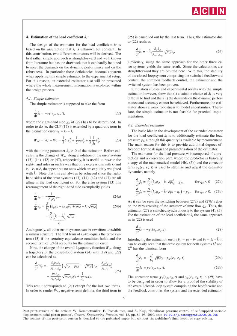
5. Measurement Results
In this section, the properties of the proposed control strategy
comprising the feedforward controller FF I (7), (9) and FF II
(11) and (12), the common feedback controller (19) and the ex-
tended estimator (37) and (38), are analyzed by means of mea-
surement results of a test stand. The test stand was designed and
built by the company HYDAC Electronic GmbH, see Fig. 3.
The main components of this test stand are the variable dis-
placement axial piston pump driven by an induction machine
and controlled by the control valve, the load volume and the
load orifice. The schematic diagram of the hydraulic circuit of
the test stand is given in Fig. 2 and the parameters of the system
are summarized in Table 1.
axial piston pump
induction machineload orifice
control valve
Figure 3: Experimental setup of the test stand for the axial piston pump.
parameter symbol value unit
bulk modulus β 1.6 · 109 Pa
eff. area of actuator Aa 300 mm2
eff. radius of actuator ra 50 mm
number of pistons np 9
area of piston Ap 165 mm2
radius of rot. of pistons rp 30 mm
angular vel. of pump ωp 50π 1s
pump coefficient kp 2.23 · 10−3 m3
s
min. swash plate angle ϕp,min −1.5 ◦
max. swash plate angle ϕp,max 18 ◦
load volume Vl 1.5 l
min. load coeff. kl,min 10 · 10−9 m3
s√
Pa
nom. load coeff. kl,nom 90 · 10−9 m3
s√
Pa
max. load coeff. kl,max 140 · 10−9 m3
s√
Pa
Table 1: Parameters of the pump and the load.
The actuator for tilting the swash plate is controlled by a (3/3)
proportional directional valve, cf. Fig. 2. In contrast to the pre-
vious assumption, the volume flow qa into the actuator cannot
be directly assigned by means of this valve. In fact, only the
position sv of the spool of the valve can be controlled directly.
7
Post-print version of the article: W. Kemmetmüller, F. Fuchshumer, and A. Kugi, “Nonlinear pressure control of self-supplied variabledisplacement axial piston pumps”, Control Engineering Practice, vol. 18, pp. 84–93, 2010. doi: 10.1016/j.conengprac.2009.09.006The content of this post-print version is identical to the published paper but without the publisher’s final layout or copy editing.
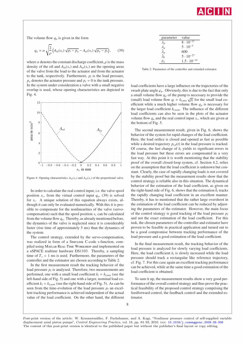
where α denotes the constant discharge coefficient, ρ is the mass
density of the oil and Ala(sv) and Aat(sv) are the opening areas
of the valve from the load to the actuator and from the actuator
to the tank, respectively. Furthermore, pl is the load pressure,
pa denotes the actuator pressure and pt = 0 is the tank pressure.
In the system under consideration a valve with a small negative
overlap is used, whose opening characteristics are depicted in
Fig. 4.
−1 −0.8 −0.6 −0.4 −0.2 0 0.2 0.4 0.6 0.8 10
2
4
6
8
10
12
sv in mm
area
inmm
2
Aat Ala
Figure 4: Opening characteristics Ala(sv) and Aat(sv) of the proportional valve.
In order to calculate the real control input, i.e. the valve spool
position sv, from the virtual control input qa, (39) is solved
for sv. A unique solution of this equation always exists, al-
though it can only be evaluated numerically. With this it is pos-
sible to compensate for the nonlinearities of the valve (servo-
compensation) such that the spool position sv can be calculated
from the volume flow qa. Thereby, as already mentioned before,
the dynamics of the valve is neglected since it is considerably
faster (rise time of approximately 5 ms) than the dynamics of
the system.
The control strategy, extended by the servo-compensation,
was realized in form of a Simulink C-code s-function, com-
piled using Matlab Real-TimeWorkshop and implemented on
a dSPACE realtime hardware DS1103. Thereby, a sampling
time of T s = 1 ms is used. Furthermore, the parameters of the
controller and the estimator are chosen according to Table 2.
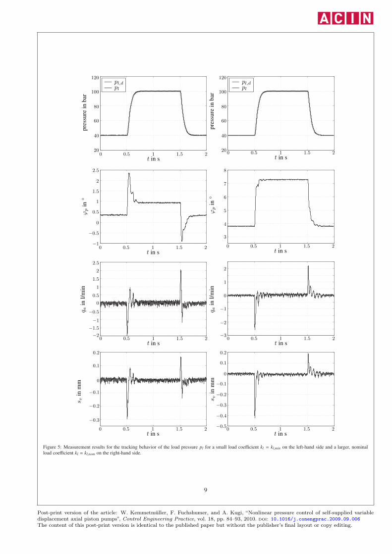
In the first measurement result the tracking behavior of the
load pressure pl is analyzed. Therefore, two measurements are
performed, one with a small load coefficient kl = kl,min (see the
left-hand side of Fig. 5) and one with a larger, nominal load co-
efficient kl = kl,nom (see the right-hand side of Fig. 5). As can be
seen from the time-evolution of the load pressure pl an excel-
lent tracking performance is achieved independent of the actual
value of the load coefficient. On the other hand, the different
parameter value
λp 8 · 10−11
λϕ 5 · 10−3
λp 600
λk 5 · 10−27
δ2 1.5 · 10−14
Table 2: Parameters of the controller and extended estimator.
load coefficients have a large influence on the trajectories of the
swash plate angle ϕp. Obviously, this is due to the fact that only
a small volume flow qp of the pump is necessary to provide the
(small) load volume flow ql = kl,min√
pl for the small load co-
efficient while a much higher volume flow qp is necessary for
the larger load coefficient kl,nom. The influence of the different
load coefficients can also be seen in the plots of the actuator
volume flow qa and the real control input sv, which are given at
the bottom of Fig. 5.
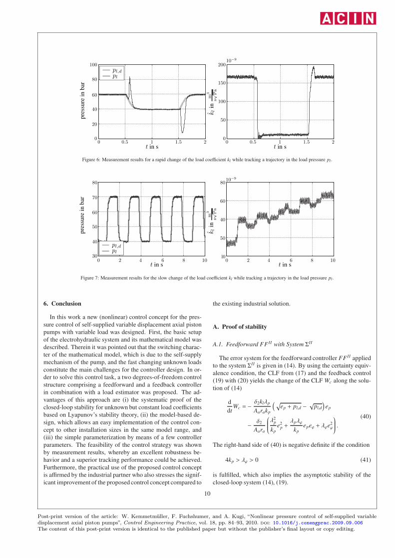
The second measurement result, given in Fig. 6, shows the
behavior of the system for rapid changes of the load coefficient.
Here, the load orifice is closed and opened as fast as possible
while a desired trajectory pl,d(t) in the load pressure is tracked.
Of course, the fast change of kl yields to significant errors in
the load pressure but these errors are compensated in a very
fast way. At this point it is worth mentioning that the stability
proof of the overall closed-loop system, cf. Section 4.2, relies
on the assumption that the load coefficient is unknown but con-
stant. Clearly, the case of rapidly changing loads is not covered
by the stability proof but the measurment results show that the
control strategy is reliable also in this situation. The dynamical
behavior of the estimation of the load coefficient, as given on
the right-hand side of Fig. 6, shows that the estimation kl tracks
the rapidly changing load coefficient in an excellent manner.
Thereby, it has to mentioned that the rather large overshoot in
the estimation of the load coefficient can be reduced by adjust-
ing the parameters of the estimator. However, the main focus
of the control strategy is good tracking of the load pressure pl
and not the exact estimation of the load coefficient. For this
task, the chosen parameters of the controller and estimator have
proven to be feasible in practical application and turned out to
be a good compromise between tracking performance of the
load pressure and a good estimation of the load coefficient.
In the final measurement result, the tracking behavior of the
load pressure is analyzed for slowly varying load coefficients.
Here, the load coefficient kl is slowly increased while the load
pressure should track a rectangular like reference trajectory,
cf. Fig. 7. For this case again an excellent tracking performance
can be achieved, while at the same time a good estimation of the
load coefficient is obtained.
To sum it up, the measurement results show a very good per-
formance of the overall control strategy and thus prove the prac-
tical feasibility of the proposed control strategy comprising the
feedforward control, the feedback control and the extended es-
timator.
8
Post-print version of the article: W. Kemmetmüller, F. Fuchshumer, and A. Kugi, “Nonlinear pressure control of self-supplied variabledisplacement axial piston pumps”, Control Engineering Practice, vol. 18, pp. 84–93, 2010. doi: 10.1016/j.conengprac.2009.09.006The content of this post-print version is identical to the published paper but without the publisher’s final layout or copy editing.
Figure 5: Measurement results for the tracking behavior of the load pressure pl for a small load coefficient kl = kl,min on the left-hand side and a larger, nominal
load coefficient kl = kl,nom on the right-hand side.
9
Post-print version of the article: W. Kemmetmüller, F. Fuchshumer, and A. Kugi, “Nonlinear pressure control of self-supplied variabledisplacement axial piston pumps”, Control Engineering Practice, vol. 18, pp. 84–93, 2010. doi: 10.1016/j.conengprac.2009.09.006The content of this post-print version is identical to the published paper but without the publisher’s final layout or copy editing.
Figure 6: Measurement results for a rapid change of the load coefficient kl while tracking a trajectory in the load pressure pl.
l000 22 44 66 88 1010
30
40
40
50
60
60
70
8080
t in st in s
pre
ssu
rein
bar
pl,dpl
50
10−9
kl
inm
3
s√Pa
Figure 7: Measurement results for the slow change of the load coefficient kl while tracking a trajectory in the load pressure pl.
6. Conclusion
In this work a new (nonlinear) control concept for the pres-
sure control of self-supplied variable displacement axial piston
pumps with variable load was designed. First, the basic setup
of the electrohydraulic system and its mathematical model was
described. Therein it was pointed out that the switching charac-
ter of the mathematical model, which is due to the self-supply
mechanism of the pump, and the fast changing unknown loads
constitute the main challenges for the controller design. In or-
der to solve this control task, a two degrees-of-freedom control
structure comprising a feedforward and a feedback controller
in combination with a load estimator was proposed. The ad-
vantages of this approach are (i) the systematic proof of the
closed-loop stability for unknown but constant load coefficients
based on Lyapunov’s stability theory, (ii) the model-based de-
sign, which allows an easy implementation of the control con-
cept to other installation sizes in the same model range, and
(iii) the simple parameterization by means of a few controller
parameters. The feasibility of the control strategy was shown
by measurement results, whereby an excellent robustness be-
havior and a superior tracking performance could be achieved.
Furthermore, the practical use of the proposed control concept
is affirmed by the industrial partner who also stresses the signif-
icant improvement of the proposed control concept compared to
the existing industrial solution.
A. Proof of stability
A.1. Feedforward FF II with System ΣII
The error system for the feedforward controller FF II applied
to the system ΣII is given in (14). By using the certainty equiv-
alence condition, the CLF from (17) and the feedback control
(19) with (20) yields the change of the CLF Wc along the solu-
tion of (14)
d
dtWc = −
δ2klλp
Aarakp
( √ep + pl,d − √pl,d
)ep
− δ2
Aara
λ2
p
kp
e2p +λpλϕ
kp
epeϕ + λϕe2ϕ
.(40)
The right-hand side of (40) is negative definite if the condition
4kp > λϕ > 0 (41)
is fulfilled, which also implies the asymptotic stability of the
closed-loop system (14), (19).
10
Post-print version of the article: W. Kemmetmüller, F. Fuchshumer, and A. Kugi, “Nonlinear pressure control of self-supplied variabledisplacement axial piston pumps”, Control Engineering Practice, vol. 18, pp. 84–93, 2010. doi: 10.1016/j.conengprac.2009.09.006The content of this post-print version is identical to the published paper but without the publisher’s final layout or copy editing.
Krstic M., Kanellakopoulos I. & Kokotovic P. (1995) Nonlinear and Adaptive
Control Design. New York: John Wiley & Sons.
Liberzon D. (2003) Switching in Systems and Control. Boston, USA:
Birkhauser.
Manring N.D. & Johnson R.E. (1996) Modeling and designing a variable-
displacement open-loop pump. ASME J. of Dynamic Systems, Measurement
and Control, 118(2), 267-271.
Manring N.D. (2005) Hydraulic Control Systems. New Jersey, USA: John Wi-
ley & Sons.
McCloy D. & Martin H.R. (1980) Control of Fluid Power: Analysis and De-
sign. New York: John Wiley & Sons.
Merritt H.E. (1967) Hydraulic Control Systems. New York: John Wiley & Sons.
Wu D., Burton R., Schoenau G. & Bitner D. (2002) Establishing operating
points for a linearized model of a load sensing system. Int. Journal of Fluid
Power, 3(2), 47-54.
11
Post-print version of the article: W. Kemmetmüller, F. Fuchshumer, and A. Kugi, “Nonlinear pressure control of self-supplied variabledisplacement axial piston pumps”, Control Engineering Practice, vol. 18, pp. 84–93, 2010. doi: 10.1016/j.conengprac.2009.09.006The content of this post-print version is identical to the published paper but without the publisher’s final layout or copy editing.


![Nonlinear control systems[1]](https://static.documents.pub/doc/80x56/5561fd91d8b42a25488b507e/nonlinear-control-systems1.jpg)