Nonlinear Pricing Kernels, Kurtosis Preference, and Evidence...

Nonlinear Pricing Kernels,Kurtosis Preference, and Evidence

from the Cross Sectionof Equity Returns

ROBERT F. DITTMAR*

ABSTRACT

This paper investigates nonlinear pricing kernels in which the risk factor is en-dogenously determined and preferences restrict the definition of the pricing ker-nel. These kernels potentially generate the empirical performance of nonlinear andmultifactor models, while maintaining empirical power and avoiding ad hoc spec-ifications of factors or functional form. Our test results indicate that preference-restricted nonlinear pricing kernels are both admissible for the cross section ofreturns and are able to significantly improve upon linear single- and multifactorkernels. Further, the nonlinearities in the pricing kernel drive out the importanceof the factors in the linear multi-factor model.

A PRINCIPAL IMPLICATION OF THE Capital Asset Pricing Model ~CAPM! is thatthe pricing kernel is linear in a single factor, the portfolio of aggregate wealth.Numerous studies over the past two decades have documented violations ofthis restriction.1 In response, researchers have examined the performance ofalternative models of asset prices. These models have generally fallen intotwo classes: ~1! multifactor models such as Ross’ APT or Merton’s ICAPM, inwhich factors in addition to the market return determine asset prices; or~2! nonparametric models, such as Bansal et al. ~1993!, Bansal andViswanathan ~1993!, and Chapman ~1997!, in which the pricing kernel is not

* Dittmar is at the Kelley School of Business, Indiana University, Bloomington, Indiana.This paper is based on the author’s dissertation at the University of North Carolina. Thanksto Dong-Hyun Ahn, Ravi Bansal, Utpal Bhattacharya, Mike Cliff, Jennifer Conrad, Amy Ditt-mar, Wayne Ferson, Ron Gallant, the journal editor, Richard Green, Mustafa Gültekin, Camp-bell Harvey, Karl Lins, Steve Monahan, Steve Slezak, George Tauchen, Marc Zenner, and ananonymous referee for valuable comments. Thanks also to seminar participants at Case West-ern Reserve University; Indiana University; the Office of the Comptroller of the Currency;Penn State University; the 1999 Western Finance Association meetings ~Santa Monica!; andthe Universities of Cincinnati, Miami, Minnesota, North Carolina, Utah, Virginia, and West-ern Ontario for helpful comments and discussions. The author also thanks Eugene Fama andKenneth French for making their data available. Any remaining errors are solely the author’sresponsibility.

1 The literature documenting violations of this restriction is voluminous. A comprehensiveset of references may be found in Campbell, Lo, and MacKinlay ~1995!.

THE JOURNAL OF FINANCE • VOL. LVII, NO. 1 • FEB. 2002

369

linear in the market return. Empirical applications of these models suggestthat they are much better at explaining cross-sectional variation in expectedreturns than the CAPM.2

Although these approaches perform well empirically, a number of limita-tions weaken their appeal. In particular, the models require ad hoc specifi-cations of either the set of priced factors or the form of nonlinearity. Sincethe sets of potential factors and nonlinear functions are large, the researcherhas considerable discretion over the form of the model to be investigated.Additionally, the form of the pricing kernel resulting from the nonparamet-ric approaches does not derive from first principles. That is, given a set ofassumptions on investors’ preferences or return distributions, the nonlinearpricing kernels investigated in the nonparametric approaches do not followendogenously. These limitations of the nonparametric and multifactor ap-proaches are problematic in empirical applications because ~1! tests basedon ad hoc assumptions may lack power since they ignore the theoreticalrestrictions that might arise from a structural model and ~2! the possibilityexists for overfitting the data and factor dredging ~Lo and MacKinlay ~1990!,Fama ~1991!!. In contrast, the set of factors in the CAPM ~the market port-folio! and the form of the pricing kernel ~linear! obtain as endogenous out-comes. Thus, the CAPM is free of the criticisms of arbitrary factor andfunctional form specification.

This paper investigates a pricing kernel that retains many of the attrac-tive features of the pricing kernels investigated in nonparametric analyseswhile avoiding many of their limitations. The basis of our approach is toapproximate an unknown marginal utility function in a static setting by aTaylor series expansion. The resulting pricing kernel is a polynomial func-tion in aggregate wealth. The form of this Taylor series is restricted by im-posing decreasing absolute prudence ~Kimball ~1993!! on investor’s preferences.This restriction allows us to sign the first three polynomial terms in theexpansion. The resulting pricing kernel is nonlinear, and therefore consis-tent with empirical evidence from nonparametric studies. Furthermore, it isa function of a risk factor that obtains endogenously and is restricted bypreference assumptions, as in the CAPM. Consequently, the pricing kernelhas the potential to explain some of the observed nonlinearities in the data.Concurrently, specification tests have improved power due to the preferencerestrictions imposed on the functional form of the pricing kernel.

As discussed above, our pricing kernel is a function only of the return onaggregate wealth. However, several recent papers have shown that the spec-ification of aggregate wealth impacts the conclusions of empirical asset pric-ing studies. Consequently, we specify the priced factor as a function of boththe return on equity and the return on human capital. We incorporate hu-man capital, since recent evidence ~Campbell ~1996!, Jagannathan and Wang

2 Fama and French ~1993, 1995, 1996! propose and investigate a multifactor alternative tothe CAPM and find that it can capture more variation in expected returns than the CAPM.Bansal and Viswanathan ~1993! and Bansal et al. ~1993! explore various nonlinear pricingkernel specifications and find that these nonlinear specifications outperform linear specifications.

370 The Journal of Finance

~1996!! suggests that the incorporation of human capital into the pricingkernel substantially improves the performance of the conditional CAPM. Incontrast to this work, our pricing kernel allows human capital to impactasset prices nonlinearly through the polynomial pricing kernel. Moreover,we conjecture that mismeasurement of the market portfolio may have a par-ticularly severe effect on the analysis of a nonlinear pricing kernel.

Our results indicate several interesting findings. First, we find that botha quadratic and a cubic pricing kernel are admissible for the cross section ofindustry portfolios, whereas the linear single-factor ~CAPM! and linear multi-factor ~Fama-French! pricing kernels are not. Although the superior perfor-mance of nonlinear pricing kernels to linear pricing kernels has beendocumented in the literature ~Bansal and Viswanathan ~1993!, Bansal et al.~1993!, Chapman ~1997!!, to our knowledge the superiority of these kernelsto a f lexible multifactor model, such as the Fama–French model, has not. Wefind this result particularly interesting because the nonlinear pricing kernelthat we investigate is subject to economic restrictions that do not affect themultifactor pricing kernel. In particular, the priced risk factor is obtainedendogenously, and the signs of the coefficients of the pricing kernel are re-stricted by preference theory. In contrast, the priced risk factors in the multi-factor model are specified exogenously, and the sign of the relationship betweenreturns and these risk factors is unconstrained by economic theory. Further-more, when the pricing kernel is specified as a cubic function of aggregatewealth augmented by the Fama–French factors, we find that these factorshave no residual explanatory power for the cross section of returns. Theseresults are important because they show that a pricing kernel grounded inpreference theory can perform as well as, or better than, less restrictivefactor models. Importantly, we find that human capital is critical to theimproved performance of a nonlinear pricing kernel over linear single andmultifactor pricing kernels. Moreover, it is incorporation of a nonlinear hu-man capital measure that renders the pricing kernel admissible.

Although the pricing kernel that we investigate is restricted by prefer-ences relative to multifactor or nonparametric pricing kernels, the kernelcan be restricted further by preference theory. For example, specific prefer-ences such as power utility are consistent with the decreasing absolute pru-dence restriction. We find that the nonlinear pricing kernel outperforms apricing kernel implied by power utility. This evidence leads us to investigatethe degree to which we can restrict the pricing kernel to be consistent withpreferences and maintain improvement over the multifactor pricing kernels.In particular, we note that, under the assumption of decreasing absoluterisk aversion, the pricing kernel itself should be decreasing. We impose thisconstraint in estimation and find that the resulting pricing kernel is nolonger admissible for the cross section of returns. However, this pricing ker-nel continues to outperform the linear single and multifactor pricing ker-nels. This evidence suggests that nonlinearity can augment the performanceof the pricing kernel framework. However, in order to describe the data, thepricing kernel must exhibit a fairly specific form of nonlinearity, which iscaptured by the cubic pricing kernel. Unfortunately, the cubic pricing kernel

Nonlinear Pricing Kernels 371

cannot simultaneously deliver the nonlinearity necessary to price the assetsunder consideration and monotonically decrease. We conclude that a func-tional form that is able to maintain both of these properties is necessary tobe both economically reasonable and admissible.

The remainder of the paper is organized as follows. In Section I, we dis-cuss and motivate restrictions on agents’ preferences that yield a specificnonlinear pricing kernel. The testing framework is discussed in Section II.Evidence on the performance of the model is provided in Section III. Sec-tion IV concludes.

I. Pricing Kernels and Moment Preference

To develop a specific nonlinear pricing kernel, we start with the intertem-poral consumption and portfolio choice problem for a long-lived investor. Asdiscussed in Hansen and Jagannathan ~1991!, the solution to an investor ’sportfolio choice problem can be expressed as the Euler equation

E @~1 � Ri, t�1!mt�16�t # � 1, ~1!

where ~1 � Ri, t�1! is the total return on asset i; mt�1 is the investor ’s in-tertemporal marginal rate of substitution, U '~Ct�1!0U

'~Ct !; and �t is theinformation set available to the investor at time t. Harrison and Kreps ~1979!show that mt�1 represents a pricing kernel that prices all risky payoffs un-der the law of one price and is nonnegative under the condition of no arbi-trage. The assumption of the existence of a representative agent allows thepricing kernel to be expressed as a function of aggregate consumption. Al-though this specification is appealing from the standpoint of economic theory,considerable attention has been given to measurement and aggregation prob-lems in available aggregate consumption proxies ~e.g., Breeden, Gibbons,and Litzenberger ~1989!!. One method that is used to address this issue is toassume a static setting, and allow equation ~1! to hold conditionally, as inBrown and Gibbons ~1985!. In this case, consumption and wealth are equiv-alent, and the intertemporal marginal rate of substitution can be expressedas a function of aggregate wealth, U '~Wt�1!0U

'~Wt !.A further issue in this analysis is the form of the representative agent’s

utility function, U~{!. A large body of literature investigates standard choicesfor U~{! and finds that the data imply unrealistic assumptions about inves-tors’ risk aversion or the riskless rate ~e.g., Mehra and Prescott ~1985!, Weil~1989!!. Thus, a suitable representation for the representative agent’s utilityfunction is unknown. To mitigate this problem, we express the pricing ker-nel generally as a nonlinear function of the return on aggregate wealth.Specifically, rather than take a stand on the exact form of the pricing ker-nel, we approximate it using a Taylor series expansion:

mt�1 � h0 � h1

U ''

U ' RW, t�1 � h2

U '''

U ' RW, t�12 � . . . , ~2!


where RW, t�1 represents the return on end-of-period aggregate wealth. Asshown in equation ~2!, the marginal rate of substitution can be approxi-mated as a polynomial in aggregate wealth in a static setting.

One difficulty with the polynomial expansion is the determination of theorder at which the expansion should be truncated. Bansal et al. ~1993! letthe data determine the point of truncation. The difficulty with this approachis a loss of power; in allowing the data to guide the specification of thepricing kernel, the researcher risks overfitting the data. Furthermore, theeconomic interpretation of the resulting kernel is open to question. A morepowerful alternative is to allow preference theory to guide the truncation.Thus, we rely on preference arguments to motivate the truncation of thepolynomial. The standard arguments of positive marginal utility and riskaversion suggest that U ' � 0 and U '' � 0. These restrictions yield a linearpricing kernel with a negative coefficient on the return on aggregate wealth,nesting the static CAPM. We further assume decreasing absolute risk aver-sion, which implies U ''' � 0, as shown in Arditti ~1967!. This condition, cou-pled with truncating the series expansion after the quadratic term, yields apricing kernel quadratic in the return on aggregate wealth, consistent withthe three-moment CAPM.

We extend this progression of signing derivatives of utility functions byusing the restriction of decreasing absolute prudence ~Kimball ~1993!!. Kim-ball develops this restriction in response to Pratt and Zeckhauser ~1987!,who show that decreasing absolute risk aversion does not rule out certaincounterintuitive risk-taking behavior. For example, any risk-averse agentshould be unwilling to accept a bet with a negative expected payoff. Samuel-son ~1963! proves that if this agent had already accepted a bet with a neg-ative expected payoff, that she should be unwilling to take another independentbet with a negative expected payoff. Pratt and Zeckhauser show that, if theagent’s preferences are restricted only to exhibit decreasing absolute riskaversion, the agent may be willing to take this negative mean sequentialgamble. Kimball shows that standard risk aversion rules out the aforemen-tioned behavior. Sufficient conditions for standard risk aversion are decreas-ing absolute risk aversion and decreasing absolute prudence,

�

dU '''

U ''

dW�~U ''' !2 � U ''''U ''

~U '' !2� 0. ~3!

Thus, assuming increasing marginal utility, risk aversion, and decreasingabsolute risk aversion, equation ~3! implies

U '''' � 0. ~4!

This condition shows that, by imposing standard risk aversion on agents’preferences, we are able to sign the coefficients of the first three polynomialterms in a Taylor series expansion.


Because preference theory does not guide us in determining the sign ofadditional polynomial terms, we assume that higher order polynomial termsare not important for pricing. More specifically, we implicitly assume thatthe covariance between returns and polynomial terms in aggregate wealth oforder greater than three is zero.3 Without this assumption, higher orderterms, which we cannot definitively sign, enter the pricing kernel. Our viewis that the power delivered by the sign restrictions outweigh the cost ofomitting the higher order polynomial terms. Thus, with the assumption thatthe pricing kernel can be characterized by a low-order polynomial in aggre-gate wealth, imposing standard risk aversion on agents’ preferences and trun-cating the expansion at the highest order term that can be signed togetherresult in a pricing kernel that is cubic in the return on aggregate wealth.4The resulting pricing kernel is decreasing in the linear term of the pricingkernel, increasing in the quadratic term, and decreasing in the cubic term.

The pricing kernel that results from our analysis has several attractivefeatures. First, the resulting pricing kernel does not take a strong standregarding functional form. Additionally, the pricing kernel is nonlinear. Con-sequently, we conjecture that the polynomial pricing kernel will avoid prob-lems associated with assuming a specific utility function and, instead, capturenonlinear features of the data, as do nonparametric pricing kernels. How-ever, in contrast to the nonparametric kernels, the polynomial model is re-stricted by preference theory; preference assumptions drive the signs of thepricing kernel coefficients. These restrictions deliver greater economic andstatistical power to tests of the model. In the subsequent sections, we con-duct analyses of the performance of this kernel relative to alternative spec-ifications of the pricing kernel.

As alluded to above, the polynomial expansion is also appealing in that itcan be linked to preference for moments of the distribution of the return onwealth. Using the definition of covariance, equation ~1! can be rewritten as

E @~1 � Ri, t�1!# �1

E @mt�1#� Cov@~1 � Ri, t�1!, mt�1#

1

E @mt�1#. ~5!

Substituting equation ~2! into equation ~5! shows that expected returns arelinked to covariances with the different orders of the polynomial in the re-turn on aggregate wealth. Thus, a linear pricing kernel relates expectedreturns to covariance with the return on aggregate wealth, as in the CAPM.A quadratic pricing kernel relates expected returns to covariance with thereturn on aggregate wealth and the return on aggregate wealth squared.Since the coskewness of a random variable x with another random variable ycan be represented as a function of Cov~x, y! and Cov~x, y2 !, the quadraticpricing kernel is consistent with the three-moment CAPM. Similarly, a cubic

3 This assumption may be justified if the joint distribution of returns and wealth is charac-terized by a four-moment density.

4 This pricing kernel is consistent with a four-moment CAPM, as derived in Fang and Lai~1997!.


pricing kernel is consistent with a model in the CAPM framework in whichagents have preference over the first four moments of returns.

Analagous arguments can be made for higher moments; the pricing kernelin Bansal et al. ~1993! incorporates a linear, quadratic, and quintic term,implying preference over variance, skewness, and the sixth moment. How-ever, moments beyond the fourth are difficult to interpret intuitively andare not explicitly restricted by standard preference theory. In contrast, pref-erence for the fourth moment, kurtosis, has both a utility-based and anintuitive rationale. Kurtosis can be described as the degree to which, for agiven variance, a distribution is weighted toward its tails ~Darlington ~1970!!.That is, kurtosis measures the bimodality of the distribution, or the proba-bility mass in the tails of the distribution. Thus, kurtosis is distinguishedfrom the variance, which measures the dispersion of observations from themean, in that it captures the probability of outcomes that are highly diver-gent from the mean; that is, extreme outcomes. In a multivariate distribu-tion, random variables may also exhibit cokurtosis. This measure capturesthe two variables’ common sensitivity to extreme states.

Thus, a cubic pricing kernel can be justified under intuitive arguments,which suggests that investors are averse to extreme outcomes in a distribu-tion, as well as utility-based arguments such as standard risk aversion. Con-sequently, we investigate a version of equation ~2! that truncates the expansionat the return on aggregate wealth cubed

mt�1 � d0 � d1 RW, t�1 � d2 RW, t�12 � d3 RW, t�1

3 . ~6!

A pricing kernel specified in this way allows for an alternative functionalform and potentially greater generality than that implied by the use of aspecific utility function. However, since signs of the coefficients in the ex-pansion are guided by theory, and we have limited the order of the expansionrather than allowing the data to determine the order of the expansion, weexpect tests of the kernel’s specification to be more powerful than a purenonparametric approach.

II. Estimation Methods

As expressed in equation ~6!, the pricing kernel is a random variable withstatic coefficients. However, a large body of evidence suggests that return mo-ments and prices of risk are time varying, and a wide array of studies haveused this evidence as a basis for investigating static pricing models that holdconditionally ~e.g., Harvey ~1989!, Ferson and Harvey ~1991!!. Although a staticmodel will not hold conditionally in general, it may under certain conditions.For example, Campbell ~1996! provides evidence that assets’ intertemporal risksare proportional to their market risk. In this case, the asset pricing model canbe expressed as a function only of market risk, allowing a static model to holdconditionally. Consequently, we analyze the model in conditional form by test-ing the implications of the Euler equation ~1!.


One potential implication of equation ~1! holding conditionally is that thecoefficients of the pricing kernel, dn, are time varying. In a full-f ledgedpricing model, the conditional moments that drive these coefficients mightbe directly modeled ~e.g., Harvey ~1989!!. Alternatively, in the more generalsituation described by ~6!, a functional form for the coefficients may be spec-ified. Dumas and Solnik ~1995! and Cochrane ~1996! treat these coefficientsas linear functions of time t information variables. The resulting pricingkernel is specified as

mt�1 � d0' Zt � d1

' Zt RW, t�1 � d2' Zt RW, t�1

2 � d3' Zt RW, t�1

3 . ~7!

This approach is advantageous in being a parsimonious approximation, butthe functional form does not impose any restrictions on the signs of thecoefficients. Consequently, we investigate a pricing kernel of the form

mt�1 � ~d0' Zt!

2 � ~d1' Zt!

2RW, t�1 � ~d2' Zt!

2RW, t�12 � ~d3

' Zt!2RW, t�1

3 . ~8!

As discussed in Section I, imposing decreasing absolute prudence impliesthat U '''' � 0, U ''' � 0, and U '' � 0. Because the coefficients ~dn, t !

2 areforced to be positive-valued in equation ~8!, this specification forces the pref-erence restrictions implied by decreasing absolute prudence.

One more feature of the pricing kernel framework is exploited in estima-tion. Equation ~1! implies that the mean of the pricing kernel should beequal to the inverse of the gross return on a riskless asset or, more generally,a zero-beta asset. That is, Et @mt�1# � 10Et @R0, t�1# . This condition can beimposed by including a proxy for the riskless or zero-beta asset in the set ofpayoffs. Dahlquist and Söderlind ~1999! and Farnsworth et al. ~1999! findthat imposing this restriction on the pricing kernel is important in the con-text of performance evaluation. Dahlquist and Söderlind also show that fail-ure to impose this restriction can result in estimation of a valid pricingkernel that implies a mean-variance tangency portfolio that is not on theefficient frontier. To impose the mean restriction on the pricing kernel, weinclude a moment condition for the one-month T-bill in the estimation.

A. Estimating the Pricing Kernel

Using the Taylor series approximation with time-varying coefficients, equa-tion ~8!, the Euler equation ~1! can be expressed as

E @~1 � Rt�1!~~d0' Zt !

2 � ~d1' Zt !

2Rm, t�1 � ~d2' Zt !

2Rm, t�12 � ~d3

' Zt !2Rm, t�1

3 !6Zt #

� 1N . ~9!

We collect the vector of errors

vt�1 � ~1 � Rt�1!~~Ztd0!2 � ~Ztd1!

2Rm, t�1 � ~Ztd2!2Rm, t�1

2 � ~Ztd3!2Rm, t�1

3 !

� 1N . ~10!


Equation ~9! implies

E @vt�16Zt # � 0, ~11!

which forms a set of moment conditions that can be utilized to test the assetpricing model via Hansen’s ~1982! generalized method of moments ~GMM!.Equation ~11! implies the unconditional restriction E @vt�1 � Zt # � 0. Thesample version of this condition is that

gT ~d! �1

T (t�1

T

vt�1 � Zt' � 0N . ~12!

T represents the number of time series observations and N the number ofassets under consideration. Expression ~12! is a system of N � K equations.The number of parameters in the model, p, is driven by the restrictions onequation ~7!. In the cubic case, p � 4K, whereas in the quadratic and linearcases, p � 3K and 2K, respectively.

Hansen ~1982! shows that a test of model specification can be obtained byminimizing the quadratic form

J~d! � gT ~d!'WT ~d!gT ~d!, ~13!

where WT is the GMM weighting matrix. Alternative approaches to GMMestimation are based on the specification of the weighting matrix. Hansenshows that the optimal weighting matrix is the covariance matrix of themoment conditions, WT

* � @gT ~d!gT' ~d!#�1 . Although the GMM estimates with

respect to this matrix are efficient, several studies ~e.g., Ferson and Foerster~1994!! suggest that the method may have poor finite sample properties.Furthermore, as pointed out in Chapman ~1997!, since the weighting matrixis the inverse of the second moment matrix of the pricing errors, a smallJ-statistic can be obtained through estimating a pricing kernel with highlyvolatile pricing errors. Thus, using the standard GMM estimator in an Eulerequation test may result in acceptance of a pricing kernel due not to im-proved pricing ability, but instead due to the addition of noise to the pricingkernel.

Hansen and Jagannathan ~1997! pursue a different approach. Rather thanattempting to minimize the pricing errors weighted by their covariance ma-trix, the authors investigate the size of the correction to a model’s pricingkernel that is necessary for it to be consistent with a pricing kernel thatprices the assets. The solution to this problem uses the same criterion func-tion as the standard GMM estimator, equation ~13!, but specifies the weight-ing matrix as the second moment of instrument-scaled returns:

W HJ � E @~Rt�1 � Zt !~Rt�1 � Zt !' # . ~14!


We follow Jagannathan and Wang ~1996! and Chapman ~1997! in implement-ing this approach. The distribution of J HJ, the resulting test statistic, isderived in Jagannathan and Wang and is used as a test of model specification.

There are several advantages to using the Hansen–Jagannathan estima-tor rather than the standard GMM estimator. First, the Hansen–Jagannathanapproach provides a statistic that can be used to compare nonnested models.This statistic is termed the Hansen–Jagannathan distance measure and isgiven by the square root of the criterion function equation ~13! using theHansen–Jagannathan weighting matrix, equation ~14!. This distance mea-sure is equivalent to 66 Ip 66, where Ip is the correction to the proxy stochasticdiscount factor necessary to make it consistent with the data. Since the dis-tance measure is formed on a weighting matrix that is invariant across allmodels tested, it can be used to directly compare the performance not only ofnested models, but nonnested models as well.

A second advantage to the Hansen–Jagannathan approach is that it largelyavoids the pitfall of favoring pricing models that produce volatile pricingerrors. The Hansen–Jagannathan criterion is a function of the inverse of thesecond moment matrix of returns rather than the inverse of the second mo-ment matrix of pricing errors. Consequently, the Hansen–Jagannathan dis-tance will fall only if the least-square distance to an admissible pricing kernelis reduced, and not if the proxy pricing kernel generates volatile pricingerrors. Thus, the distance rewards models exclusively for improving pricingand not for adding noise.

One caveat is in order. The distribution of the Hansen–Jagannathan teststatistic is a function of the optimal GMM weighting matrix. Consequently,when testing the significance of the Hansen–Jagannathan distance, one mayfind a high p-value because the parameters imply a “small” optimal GMMweighting matrix; that is, a weighting matrix characterized by highly vola-tile pricing errors. One potential safeguard against failing to reject a modeldue simply to noise in the pricing kernel is to analyze the significance of theparameter estimates. Whereas the distribution of the distance measure isrewarded for a small GMM weighting matrix, the distribution of the param-eter estimates is penalized by a small GMM weighting matrix. That is, al-though a model may be accepted due to volatile pricing errors, the volatilitywill tend to reduce the significance of the parameter estimates. Conse-quently, we perform Wald tests to assess the significance of adding eachmarginal term in the pricing kernel. These tests provide some surety notonly that a pricing kernel is not rewarded simply for being noisy, but alsoprovides evidence as to the importance of adding polynomial terms, poten-tially alleviating concerns about overfitting.

A final advantage to the Hansen–Jagannathan distance measure is thatthe results may be more robust than in standard GMM estimates ~Cochrane~2001!!. Since the weighting matrix is not a function of the parameters, theresults should be more stable. Despite this advantage, Ahn and Gadarowski~1999! suggest that the size of the test statistic is poor in finite samples; thedistance measure rejects correctly specified models too often. These resultssuggest the possibility that using the Hansen–Jagannathan estimator rather


than the standard GMM estimator may trade size for power. To gauge thepossible impact of this trade-off, we also estimate the models using the it-erated GMM estimator of Hansen, Heaton, and Yaron ~1996!. Ferson andFoerster ~1994! show that the iterated GMM estimator has superior finitesample properties relative to the standard GMM estimator.5

B. Measurement of the Market Portfolio

A principal difficulty in estimating asset pricing relationships based onthe portfolio of aggregate wealth is mismeasurement of the market portfolio,as noted in Roll ~1977!. Stambaugh ~1982! addresses this issue by examiningmany different market indices and finds that they produce similar infer-ences about the CAPM, even when common stocks represent only 10 percentof the index’s value. However, Stambaugh does not investigate the impact ofincluding a measure of human capital, as suggested in Mayers ~1972!. Re-cent studies, notably Jagannathan and Wang ~1996! and Campbell ~1996!,suggest that human capital is an important determinant of the cross sectionof expected returns. Jagannathan and Wang note that dividend income rep-resents only three percent of personal income in the United States over theperiod 1959 to 1992, whereas salary and wages represent 63 percent of per-sonal income. Further, Diaz-Gimenez et al. ~1992! show that approximatelytwo-thirds of nongovernment tangible assets are owned by the householdsector and only one-third of these assets is owned by the corporate sector. Ofthe corporate-owned assets, only one-third are financed by equity. This evi-dence suggests that equity may represent as little as one-ninth of aggregatewealth, a small proportion of total wealth relative to human capital.

There are complications in attempting to incorporate human capital in thewealth portfolio proxy. Mayers ~1972! explicitly treats human capital as dif-ferent from financial capital because it is not traded. However, Jagannathanand Wang ~1996! argue that human capital can be more straightforwardlyincorporated into aggregate wealth. The authors note that part of humancapital is in fact traded or hedged in the form of home mortgages, consumerloans, life insurance, unemployment insurance, and medical insurance. Con-sequently, the authors suggest that the following representation is an ap-propriate first approximation to incorporating human capital into the portfolioof aggregate wealth:

RW, t�1 � u0 � u1 Rm, t�1 � u2 Rl, t�1, ~15!

where RW, t�1 represents the return on aggregate wealth and Rl, t�1 repre-sents the return on human capital.6 It is important, however, to note thatsince only a portion of labor income is securitized that equation ~15! repre-sents an abstraction from the more explicit approach of Mayers.

5 These results are untabulated, but are available from the author on request.6 See Jagannathan and Wang ~1996! for a more complete discussion of the assumptions nec-

essary for equation ~15! to hold.


As in Jagannathan and Wang, we define the return on human capital asa two-month moving average of the growth rate in labor income:

Rl, t�1 �Lt � Lt�1

Lt�1 � Lt�2, ~16!

where Lt denotes the difference between total personal income and dividendincome at time t. The return on human capital is a function of lagged laborincome since the data become available with a one-month delay. Jagan-nathan and Wang use this two-month moving average in an attempt to min-imize the impact of measurement errors.

To implement this method, we redefine the pricing kernel in equation ~8!as follows:

mt�1 � Zt d0 � (n�1

3

In @~Zt dn,vw!2Rvw, t�1

n � ~Zt dn, lbr !2Rl, t�1

n�1 # , ~17!

where Rvw, t�1 represents the return on the value-weighted equity portfolio,Rl, t�1 represents the growth rate in labor income, and

In � � �1 n � 1,3

1 n � 2. ~18!

We assume that the cross-products in higher order terms of the return onthe wealth portfolio are zero. When cross-products are included in the esti-mation, the qualitative conclusions of the paper do not change and the per-formance of the nonlinear models improves.

C. Data and Estimation Details

Many sets of assets have been used in the empirical asset pricing litera-ture for tests of candidate asset pricing models. In our main specificationtests, we utilize the returns on 20 industry-sorted portfolios, where the in-dustry definitions follow the two-digit SIC codes used in Moskowitz andGrinblatt ~1999! and are described in Table I. As shown by King ~1966!,industry groupings proxy the investment opportunity set well; these group-ings maximize intragroup and minimize intergroup correlations.

The choice of the instrument set Zt is motivated by two considerations.First, the instruments should be a set of variables that are able to predictasset returns. Second, the choice of instruments should be parsimonious dueto power considerations in GMM estimation ~Tauchen ~1986!!. Consequently,we consider a set of instruments, Zt � $1, rmt , dyt , yst , tbt %, where 1 denotes avector of ones, rmt is the excess return on the CRSP value-weighted index attime t, dyt is the dividend yield on the CRSP value-weighted index at timet, yst is the yield on the three-month Treasury bill in excess of the yield on


the one-month Treasury bill at time t, and tbt is the return on a Treasury billclosest to one month to maturity at time t. These variables have been shownto be predictors of future returns in various studies. The value-weightedCRSP index is examined in Harvey ~1989! and Ferson and Harvey ~1991!.Fama and French ~1988, 1989! investigate the predictive power of the divi-dend yield. Campbell ~1987! shows that term premia in Treasury bill returnscan predict stock returns. Finally, Fama and Schwert ~1977!, Ferson ~1989!,and Shanken ~1990! examine the T-bill return.

The data used to compute the industry portfolio returns, value-weightedindex return, dividend yield, yield spread, and risk-free return are obtainedfrom CRSP. The data used to compute the labor return series is obtainedfrom the NIPA data available on DataStream. Labor income at time t is

Table I

Summary Statistics: Industry PortfoliosTable I presents monthly means and standard deviations of the returns on 20 industry-sorted port-folios as in Moskowitz and Grinblatt ~1999!. Portfolios are equally weighted and formed on thebasis of two-digit SIC codes. The data cover the period July 31, 1963, through December 31, 1995.

Panel A: Mean Returns

IndustryMean

Return IndustryMean

Return

Mining 0.0128 Electrical Equipment 0.0148Food & Beverage 0.0137 Transport Equipment 0.0138Textile & Apparel 0.0112 Manufacturing 0.0138Paper Products 0.0132 Railroads 0.0140Chemical 0.0139 Other Transportation 0.0132Petroleum 0.0132 Utilities 0.0097Construction 0.0125 Department Stores 0.0113Primary Metals 0.0112 Other Retail 0.0133Fabricated Metals 0.0144 Finance, Real Estate 0.0110Machinery 0.0130 Other 0.0131

Panel B: Standard Deviations

IndustryStandard

Dev. IndustryStandard

Dev.

Mining 0.0674 Electrical Equipment 0.0740Food & Beverage 0.0495 Transport Equipment 0.0665Textile & Apparel 0.0693 Manufacturing 0.0681Paper Products 0.0575 Railroads 0.0571Chemical 0.0525 Other Transportation 0.0671Petroleum 0.0560 Utilities 0.0368Construction 0.0619 Department Stores 0.0674Primary Metals 0.0593 Other Retail 0.0626Fabricated Metals 0.0623 Finance, Real Estate 0.0575Machinery 0.0647 Other 0.0656


computed as the per capita difference between total personal income anddividend income. The data cover the period July 31, 1963, through December31, 1995, totalling 390 observations.

Sample statistics for the returns on the 20 industry portfolios and thecomponents of the market proxy are presented in Table I. The average re-turns over the sample period for the payoffs range from 101 basis points permonth for the utilities industry to 151 basis points per month for the fabri-cated metals industry. In Table II, we present a summary of the predictive

Table II

Summary Statistics: InstrumentsTable II displays a summary of the predictive power of the instrumental variables used in thepaper, Zt � $rm, t , dyt , yst , tbt % , where rm, t represents the return on the value-weighted CRSPindex, dyt is the dividend yield on the value-weighted CRSP index, yst is the excess yield on theTreasury bill closest to three months to maturity over the Treasury bill closest to one month tomaturity, and tbt is the return on the Treasury bill closest to one month to maturity. The datacover the period July 30, 1963, through December 31, 1995. The predictive power of the instru-ments is assessed by the linear projection

Ri, t�1 � d0 � dZt � ut�1.

The column labeled x42 presents Newey and West ~1987a! Wald tests of the hypothesis

H0 : d � 0

with p-values in parentheses. The statistics are computed using the Newey and West ~1987b!heteroskedasticity and autocorrelation-consistent covariance matrix.

Industry x42 Industry x4

2

Mining 13.132 Electrical Equipment 39.929~0.011! ~0.000!

Food & Beverage 24.334 Transport Equipment 39.333~0.000! ~0.000!

Textile & Apparel 32.750 Manufacturing 44.992~0.000! ~0.000!

Paper Products 22.826 Railroads 11.156~0.000! ~0.025!

Chemical 24.012 Other Transportation 19.671~0.000! ~0.001!

Petroleum 1.510 Utilities 8.522~0.825! ~0.074!

Construction 25.663 Department Stores 19.031~0.000! ~0.001!

Primary Metals 22.071 Other Retail 32.012~0.000! ~0.000!

Fabricated Metals 39.437 Finance, Real Estate 28.469~0.000! ~0.000!

Machinery 33.585 Other 37.818~0.000! ~0.000!


power of the instrumental variables for the payoffs. We project the payoffsonto the instruments:

Ri, t�1 � b'Zt � ut�1.

The table contains statistics for a Wald test of the null hypothesis that theinstruments have no predictive power for the payoffs. Consistent with theresults of previous studies, the table shows that the information variablesserve as good instruments for the payoffs.

III. Results

A. Model Specification Tests

In this section, we discuss tests of the Euler equation ~1! when the pricingkernel is expressed with quadratic time-varying coefficients, as in equation~8!. We analyze the cubic pricing kernel and also the linear and quadraticpricing kernels that are nested in the cubic case. Results are presented withand without human capital as a component of the return on aggregate wealth.

Table III presents results of specification tests when the measure of ag-gregate wealth does not include human capital. The table presents averagevalues of the coefficients dn, t , n � 1,2,3 corresponding to the nth order of thereturn on the market portfolio. The table also presents the Hansen–Jagannathan distance measure and p-values for the Hansen–Jagannathantest of model specification. The first row of each panel, labeled “Coeffi-cients,” presents the value of the estimated coefficient evaluated at the meanof the instruments. As shown in the table, with this specification, the linear,quadratic, and cubic pricing kernels are all rejected at the five percent sig-nificance level for this data set. The distance measures and p-values for thetests of significance of the coefficients suggest marginal improvement frommoving from a linear specification to a nonlinear specification. The qua-dratic pricing kernel reduces the distance measure from 0.735 to 0.709, adrop of 3.5 percent relative to the linear pricing kernel. The test of the sig-nificance of the d2 terms suggest that this improvement is marginally sig-nificant ~ p-value 0.027!, indicating that incorporation of the quadratic termin the pricing kernel improves the fit of the model. These results are con-sistent with the findings of Harvey and Siddique ~2000!. However, the ad-dition of a cubic term does not materially improve the performance of thepricing kernel.

We next analyze the impact of incorporating a measure of human capitalin the return on aggregate wealth. These results are displayed in Table IV.The outcome of the specification tests are markedly different from those inTable III. All three of the pricing kernels improve substantially relative tothe case in which human capital is not included in the measure of aggregatewealth. The distance measure implied by the linear pricing kernel falls to


0.719, a decline of 2.2 percent relative to the linear kernel omitting humancapital. This result is consistent with the findings of Jagannathan and Wang~1996!, who find that incorporating human capital improves the perfor-mance of the conditional CAPM. However, the linear pricing kernel is re-jected at the five percent significance level ~ p-value 0.019!.

Considerable further improvement is observed by moving from a linear toa nonlinear specification. The results in Panel B of Table IV indicate that aquadratic specification of the pricing kernel results in an additional de-crease in the distance measure of 12.5 percent relative to the linear kernelwith human capital. This pricing kernel cannot be rejected at the 10 percent

Table III

Specification Tests: Polynomial Pricing Kernels with HumanCapital Excluded

Table III presents results of GMM tests of the Euler equation condition,

E @~1 � Rt�1!mt�16Zt #� 1N � 0

using the polynomial pricing kernels, mt�1 nested in equation ~7!. The coefficients are esti-mated using the Hansen and Jagannathan ~1997! weighting matrix E @~Rt�1 � Zt !~Rt�1 �

Zt !' # . The columns present the coefficients of the pricing kernel evaluated at the means of the

instruments. The coefficients are modeled as

dn � In~dn' Zt !

2 In � � �1 n � 2,4

1 n � 3.

P-values for Wald tests of the joint significance of the coefficients are presented in parentheses.The final column presents the Hansen–Jagannathan distance measure with p-values for thetest of model specification in parentheses. The set of returns used in estimation are those of 20industry-sorted portfolios augmented by the return on a one-month Treasury bill, covering theperiod July 31, 1963, through December 31, 1995, and the measure of aggregate wealth doesnot include human capital.

d~ RZ!0t d~ RZ!1t d~ RZ!2t d~ RZ!3t Dist

Panel A: Linear

Coefficient 1.088 �3.936 0.735P-value ~0.000! ~0.000! ~0.000!

Panel B: Quadratic

Coefficient 0.950 �4.702 77.633 0.709P-value ~0.000! ~0.000! ~0.027! ~0.001!

Panel C: Cubic

Coefficient 0.941 �4.545 77.655 �4.647 0.703P-value ~0.000! ~0.000! ~0.053! ~0.654! ~0.000!


significance level ~p-value 0.100!. Incorporating the quadratic return on wealthterm contributes significantly to the fit of the pricing kernel, as indicated bythe test of the significance of the d2 terms ~ p-values 0.002 and 0.000!. Thus,incorporating a nonlinear function of the return on human capital appearsto have a dramatic impact on the fit of the pricing kernel.

The performance of the pricing kernel is further enhanced by incorporat-ing the cubic return on wealth, as shown in Panel C. The distance measurefalls to 0.578, a decline of 8.1 percent relative to the quadratic pricing ker-nel, and a decrease of 21.4 percent relative to the conditional CAPM esti-mated in Panel A of Table III. Moreover, the specification test cannot rejectthe cubic pricing kernel at the 10 percent significance level ~ p-value 0.229!,

Table IV

Specification Tests: Polynomial Pricing Kernels with HumanCapital Included

Table IV presents results of GMM tests of the Euler equation condition,

E @~1 � Rt�1!mt�16Zt #� 1N � 0




dn � In~dn' Zt !

2 In � � �1 n � 2,4

1 n � 3.

P-values for Wald tests of the joint significance of the coefficients are presented in paren-theses. The final column presents the Hansen–Jagannathan distance measure with p-valuesfor the test of model specification in parentheses. The set of returns used in estimation arethose of 20 industry-sorted portfolios covering the period July 31, 1963, through December 31,1995, augmented by the return on a 30-day Treasury bill. The measure of aggregate wealthincludes human capital.

d~ QZ!0t d~ QZ!1vw d~ QZ!1l d~ QZ!2vw d~ QZ!2l d~ QZ!3vw d~ QZ!3l Dist

Panel A: Linear

Coefficient 1.197 �3.674 �1.020 0.719P-value ~0.000! ~0.000! ~0.000! ~0.000!

Panel B: Quadratic

Coefficient 0.725 �3.447 �12.326 46.043 9,839.447 0.629P-value ~0.000! ~0.000! ~0.000! ~0.008! ~0.000! ~0.100!

Panel C: Cubic

Coefficient 0.392 �2.079 �0.013 74.010 17,374.873 �0.084 �72,319.964 0.578P-value ~0.000! ~0.003! ~0.001! ~0.002! ~0.000! ~0.945! ~0.000! ~0.229!


and the d3l term contributes significantly to the improvement in the dis-tance measure ~ p-value 0.000!.7 These results suggest that, by allowing forpreference restrictions implied by decreasing absolute risk aversion and de-creasing absolute prudence, that the performance of a pricing kernel groundedin preference theory can capture cross-sectional variation in returns. Theresults of Tables III and IV suggest that incorporating only nonlinear func-tions of the return on the value-weighted index or a linear function of thereturn on labor is insufficient to generate an admissible pricing kernel. How-ever, by utilizing both the return on labor and the nonlinearities implied bythe series expansion, we are able to generate an admissible pricing kernel.8

B. Multifactor Alternatives

As noted earlier in the paper, multifactor models of asset prices have beenmore successful in pricing the cross section of equities than have single-factor models. However, multifactor models provide the researcher with con-siderable freedom since the models give little guidance for the choice of factors.In contrast, the pricing kernel in this paper explicitly defines the relevantfactor for pricing, the portfolio of aggregate wealth. Further, preference theoryimposes restrictions on the signs of the coefficients on each term in thepricing kernel. In this section, we gauge the ability of the polynomial pricingkernel to price the cross section of industry portfolios relative to a popularmultifactor model, the Fama and French ~1993! three-factor model. This modelis not nested in the polynomial pricing kernel, but the performance of all ofthe models can be compared using their Hansen–Jagannathan distance mea-sures, as discussed previously.

Fama and French ~1992! provide evidence that firms’ market capitaliza-tion and market-to-book ratios appear to outperform the CAPM beta in cap-turing cross-sectional variation in returns. Fama and French ~1993!, notingthis evidence, propose the following model for returns

E @ri, t�1# � bMRP E @rMRP, t�1#� bSMB E @rSMB, t�1#� bHML E @rHML, t�1# . ~19!

In this model, rMRP, t�1 represents the excess return on the market portfolioover the risk free rate, rSMB, t�1 represents the excess return on a portfolioof small capitalization stocks over large capitalization stocks, and rHML, t�1

7 The magnitude of the average coefficient is quite large ~�7.232 � 104!. This magnitude isdriven by the size of the higher orders of the return on labor income. The mean of the monthlyreturn on labor income is 0.0057, whereas the mean of the monthly return on labor incomecubed is 4.233 � 10�7. Thus, the coefficient on the cubic term is quite large to ref lect thescaling of the return on labor income cubed.

8 In untabulated results, we repeat the estimation of the pricing kernels using the iteratedGMM estimator in Hansen et al. ~1996!. The results of this estimation mirror the Hansen–Jagannathan distance estimates. Consequently, both sets of tests suggest that nonlinear pric-ing kernels with reasonable economic restrictions perform well in pricing the cross section ofindustry-sorted returns.


represents the excess return on a portfolio of high market-to-book stocksover low market-to-book stocks.9 The authors suggest that the returns to theportfolios SMB and HML represent hedge portfolios in the sense of Merton~1973!. In later work ~Fama and French ~1995, 1996!!, the authors suggestthat the size and book-to-market factors may capture some systematic dis-tress factor. The model in expression ~19! can be expressed in stochasticdiscount factor form. As in Jagannathan and Wang ~1996!, note that equa-tion ~19! implies

mt�1FF � d0 � dMRP rMRP, t�1 � dSMB rSMB, t�1 � dHML rHML, t�1. ~20!

In this setting, the coefficients dn capture the prices of factor n risk. Weallow for time variation in these coefficients by assuming a linear specifi-cation in the instruments.10

Results for the estimation of the Fama–French model are presented inPanel A of Table V. The results suggest that the pricing kernel implied bythe model fares poorly in describing the cross section of industry returns.The distance measure for the model of 0.714 ~ p-value 0.000! is comparableto the distance measure for the linear pricing kernel incorporating humancapital. Further, the distance measure of the Fama–French model is sub-stantially higher than that of either the quadratic or the cubic pricing kernelwith human capital. Thus, the results suggest that, although preference re-strictions are imposed on the nonlinear pricing kernels and the kernels arespecified as functions of the return on aggregate wealth, the nonlinear ker-nels outperform the Fama–French model in pricing the cross section of in-dustry returns.

To further investigate the ability of the Fama–French factors to price thecross section of equity returns compared to the polynomial pricing kernels,we estimate the polynomial models augmented by the SMB and HML factorsof the Fama–French model. Results of these tests are also presented in Table V.In the case of the quadratic pricing kernel, the distance measure falls from0.629 to 0.588 with the Fama–French factors included. The p-value of thespecification test for the quadratic kernel augmented by the Fama–Frenchfactors falls to 0.040, indicating that the loss of degrees of freedom resultingfrom the incorporation of the Fama–French factors more than offsets anyimprovement in the fit of the pricing kernel. However, the SMB factor con-tinues to be marginally significant, with a p-value of 0.005. In contrast,when the Fama–French factors are included in the cubic pricing kernel, themodel cannot be rejected ~ p-value 0.140!, and neither the SMB nor the HMLcoefficients are significantly different than zero. These results suggest that,

9 We would like to thank Eugene Fama for providing these data.10 We do not investigate a specification for the factor coefficients that is quadratic in the

instruments as in equation ~8! because doing so imposes restrictions on the signs of the coef-ficients. The coefficients of the Fama–French model are not restricted in sign; consequently,imposing sign restrictions would unfairly penalize the model.


Ta

ble

V

Sp

ecif

icat

ion

Tes

ts:

Fam

a–F

ren

chP

rici

ng

Ker

nel

Tab

leV

pres

ents

resu

lts

ofG

MM

esti

mat

ion

ofth

eE

ule

req

uat

ion

rest

rict

ion

E@~

1�

Rt�

1!m

t�16Z

t#�

1 N�

0

usi

ng

the

pric

ing

kern

el,

mt�

1im

plie

dby

the

Fam

aan

dF

ren

ch~1

993!

thre

e-fa

ctor

mod

el,

asin

equ

atio

n~2

0!.

Th

eco

effi

cien

tsar

ees

tim

ated

usi

ng

the

Han

sen

and

Jaga

nn

ath

an~1

997!

wei

ghti

ng

mat

rix.

P-v

alu

esfo

rW

ald

test

sof

the

join

tsi

gnif

ican

ceof

the

coef

fici

ents

are

pres

ente

din

pare

nth

eses

.T

he

fin

alco

lum

npr

esen

tsth

eH

anse

n–

Jaga

nn

ath

andi

stan

cem

easu

re,

wit

hp-

valu

esfo

rth

ete

stof

mod

elsp

ecif

icat

ion

inpa

ren

thes

es.

InP

anel

B,

the

Fam

a–F

ren

chpr

icin

gke

rnel

isau

gmen

ted

bya

quad

rati

cfu

nct

ion

ofth

ere

turn

onw

ealt

h,

and

inP

anel

B,

the

pric

ing

kern

elis

augm

ente

dby

both

aqu

adra

tic

and

acu

bic

fun

ctio

nof

the

retu

rnon

wea

lth

.T

he

set

ofre

turn

su

sed

ines

tim

atio

nar

eth

ose

of20

indu

stry

-sor

ted

port

foli

osco

veri

ng

the

peri

odJu

ly31

,19

63,

thro

ugh

Dec

embe

r31

,19

95,

augm

ente

dby

the

retu

rnon

aon

e-m

onth

Tre

asu

rybi

ll.

d~R Z! 0

td~R Z! m

rp,t

d~R Z! s

mb

,td~R Z! h

ml,

td~R Z! 1vw

d~R Z! 1

ld~R Z! 2vw

d~R Z! 2

ld~R Z! 3vw

d~R Z! 3

lD

ist

Pan

elA

:F

ama–

Fre

nch

Fac

tors

On

ly

Coe

ffic

ien

t1.

147

�5.

299

�5.

929

�1.

977

0.63

2P

-val

ue

~0.0

00!

~0.0

45!

~0.0

00!

~0.0

69!

~0.0

08!

Pan

elB

:Q

uad

rati

cA

ugm

ente

dby

Fam

a–F

ren

chF

acto

rs

Coe

ffic

ien

t1.

252

1.04

4�

0.97

0�

3.29

8�

5.66

557

.803

205.

206

0.58

8P

-val

ue

~0.0

00!

~0.0

05!

~0.5

25!

~0.0

00!

~0.0

00!

~0.0

00!

~0.0

00!

~0.0

40!

Pan

elC

:C

ubi

cA

ugm

ente

dby

Fam

a–F

ren

chF

acto

rs

Coe

ffic

ien

t0.

404

0.73

51.

766

�2.

167

�1.

146

87.8

1816

,510

.940

�0.

486

�62

,684

.668

0.55

5P

-val

ue

~0.0

00!

~0.6

21!

~0.9

41!

~0.0

05!

~0.0

00!

~0.0

20!

~0.0

00!

~0.9

99!

~0.0

00!~0

.140!


in the cross section of industry-sorted portfolios, the cubic pricing kernelcaptures much of the variation in returns that is explained by the Fama–French factors. This result is particularly interesting since the signs of thecoefficients are restricted by preference theory, and the factor obtains fromfirst principles.

C. Comparison with Power Utility

In the previous sections, we investigate models that are restricted to beconsistent with established assumptions governing agents’ preferences. How-ever, the polynomial pricing kernels that are investigated in this paper aredivorced from the more rigorous restrictions imposed by assuming a specificutility function. Caballé and Pomansky ~1996! show that all HARA utilityfunctions display standard risk aversion, consistent with the cubic pricingkernel. In this section, we assume that agents’ preferences are characterizedby power utility, and investigate the ability of the resulting pricing kernel toexplain cross-sectional variation in returns, as in Brown and Gibbons ~1985!.In doing so, we examine the trade-offs between this parsimonious specifica-tion of the pricing kernel and the more general specification implied by theTaylor series expansion.

Brown and Gibbons ~1985! investigate a static setting in which a repre-sentative agent exhibits power utility. In this case, the pricing kernel can beexpressed as

mt�1 � a0~1 � RW, t�1!�a1, ~21!

where a1 is the representative agent’s relative risk aversion. One issue inthe implementation of equation ~21! is the incorporation of human capital.In estimation, the optimization of the Euler equation is ill behaved when weallow RW, t�1 to be an unrestricted linear function of the return on labor andthe return on the value-weighted index, as in equation ~15!. Consequently,similar to Campbell ~1996!, we assume that the return on wealth can beexpressed as

RW, t�1 � a2 Rm, t�1 � ~1 � a2!Rl, t�1. ~22!

Although this formulation imposes additional restrictions on the relation-ship between returns, the value-weighted portfolio, and the labor return, itoffers a straightforward way to incorporate human capital in the pricingkernel expression ~21!.

Results of this estimation are presented in Table VI. As shown in thetable, the pricing kernel implied by power utility is rejected via the Hansen–Jagannathan distance measure both with and without human capital. Theseresults are qualitatively similar to those of Hansen and Jagannathan ~1997!,who use the distance measure to evaluate the power utility pricing kerneldefined over aggregate consumption. Both forms of the pricing kernel per-


form worse than the linear pricing kernel. Further, the incorporation of hu-man capital in the pricing kernel does not appear to materially improve theperformance of the power utility pricing kernel and seems to contribute noiseto the parameter estimates. The results suggest that although power utilityis consistent with the preference restrictions imposed on the cubic pricingkernel, the parsimony provided by a specific utility function comes at a largecost in terms of the fit of the model.11

Some intuition for the source of improvement in the performance of thepolynomial pricing kernel relative to the power utility specification is pro-vided by decomposing the distance measure as discussed in Hansen andJagannathan ~1997!. Recall from Section II.A that the distance measure canbe expressed as 66 Ip 66, where Ip is the adjustment to the model pricing kernelnecessary to reduce the distance to an admissible pricing kernel to zero.Using the definition of the norm of p, Hansen and Jagannathan note that

66 Ip 66 � !E @ Ip# 2 � Var@ Ip# . ~23!

11 The comparison between the power utility model and the polynomial models is not entirelyfair because the coefficients of the polynomial models are allowed to vary over time. In contrast,the time preference and risk aversion parameters of the power utility model are fixed. Thefocus of this paper is on conditional pricing models; however, in order to provide a fair com-parison, we estimate the polynomial models with fixed coefficients as well. The resulting dis-tance measure for the cubic pricing kernel is 0.634, compared to 0.740 for the power utilitykernel, a difference of approximately 14 percent.

Table VI

Specification Tests: Power Utility Pricing KernelTable VI presents results of GMM estimation of the Euler equation restriction

E @~1 � Rt�1!mt�16Zt #� 1N � 0

using the pricing kernel, mt�1 implied by power utility, as in equation ~21!. The coefficients areestimated using the Hansen and Jagannathan ~1997! weighting matrix. P-values for Wald testsof the significance of the coefficients are presented in parentheses. The final column presentsthe Hansen–Jagannathan distance measure, with p-values for the test of model specification inparentheses. The set of returns used in estimation are those of 20 industry-sorted portfolioscovering the period July 31, 1963, through December 31, 1995, augmented by the return on aone-month Treasury bill.

Coefficient: a0 a1 a2 Dist

Panel A: Human Capital Excluded

1.014 3.963 0.740P-value ~0.000! ~0.000! ~0.000!

Panel B: Human Capital Included

1.036 3.671 0.558 0.740P-value ~0.000! ~0.743! ~0.733! ~0.000!


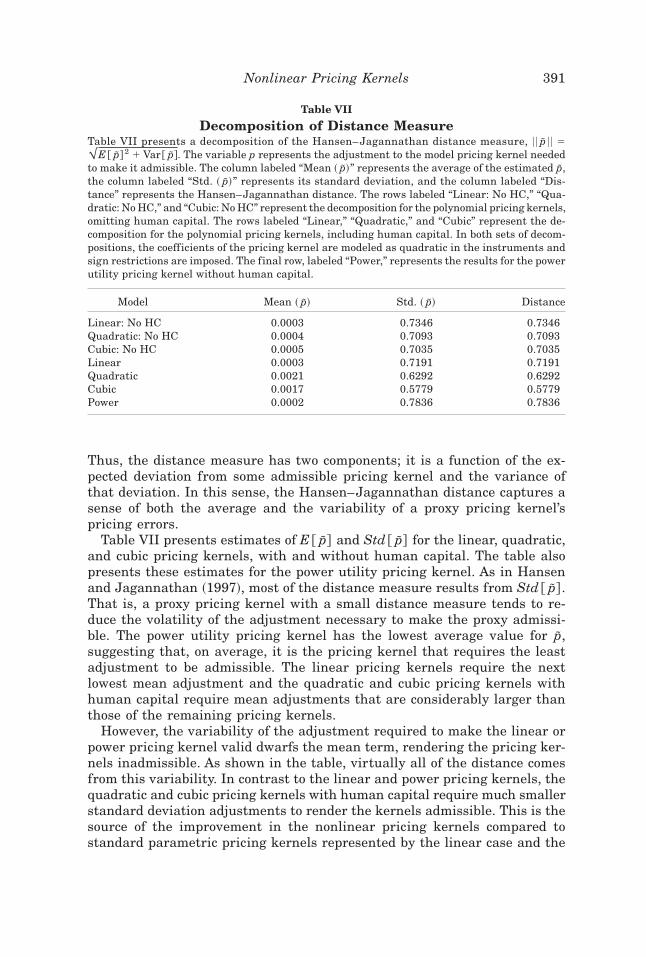
Thus, the distance measure has two components; it is a function of the ex-pected deviation from some admissible pricing kernel and the variance ofthat deviation. In this sense, the Hansen–Jagannathan distance captures asense of both the average and the variability of a proxy pricing kernel’spricing errors.

Table VII presents estimates of E @ Ip# and Std @ Ip# for the linear, quadratic,and cubic pricing kernels, with and without human capital. The table alsopresents these estimates for the power utility pricing kernel. As in Hansenand Jagannathan ~1997!, most of the distance measure results from Std @ Ip# .That is, a proxy pricing kernel with a small distance measure tends to re-duce the volatility of the adjustment necessary to make the proxy admissi-ble. The power utility pricing kernel has the lowest average value for Ip,suggesting that, on average, it is the pricing kernel that requires the leastadjustment to be admissible. The linear pricing kernels require the nextlowest mean adjustment and the quadratic and cubic pricing kernels withhuman capital require mean adjustments that are considerably larger thanthose of the remaining pricing kernels.

However, the variability of the adjustment required to make the linear orpower pricing kernel valid dwarfs the mean term, rendering the pricing ker-nels inadmissible. As shown in the table, virtually all of the distance comesfrom this variability. In contrast to the linear and power pricing kernels, thequadratic and cubic pricing kernels with human capital require much smallerstandard deviation adjustments to render the kernels admissible. This is thesource of the improvement in the nonlinear pricing kernels compared tostandard parametric pricing kernels represented by the linear case and the

Table VII

Decomposition of Distance MeasureTable VII presents a decomposition of the Hansen–Jagannathan distance measure, 66 Ip 66 �!E @ Ip# 2 � Var @ Ip#. The variable p represents the adjustment to the model pricing kernel neededto make it admissible. The column labeled “Mean ~ Ip!” represents the average of the estimated Ip,the column labeled “Std. ~ Ip!” represents its standard deviation, and the column labeled “Dis-tance” represents the Hansen–Jagannathan distance. The rows labeled “Linear: No HC,” “Qua-dratic: No HC,” and “Cubic: No HC” represent the decomposition for the polynomial pricing kernels,omitting human capital. The rows labeled “Linear,” “Quadratic,” and “Cubic” represent the de-composition for the polynomial pricing kernels, including human capital. In both sets of decom-positions, the coefficients of the pricing kernel are modeled as quadratic in the instruments andsign restrictions are imposed. The final row, labeled “Power,” represents the results for the powerutility pricing kernel without human capital.

Model Mean ~ Ip! Std. ~ Ip! Distance

Linear: No HC 0.0003 0.7346 0.7346Quadratic: No HC 0.0004 0.7093 0.7093Cubic: No HC 0.0005 0.7035 0.7035Linear 0.0003 0.7191 0.7191Quadratic 0.0021 0.6292 0.6292Cubic 0.0017 0.5779 0.5779Power 0.0002 0.7836 0.7836


power utility case. All of the pricing kernels fare relatively well in capturingthe mean of the pricing kernel, but, although the mean difference is close tozero, the linear and power kernels deviate highly from the set of admissiblepricing kernels. In contrast, the quadratic and cubic pricing kernels are closenot only on average to the set of admissible kernels, but the variability oftheir deviations is much lower.

D. Properties of the Estimated Pricing Kernels

Thus far, we have imposed conditions on the coefficients of the pricingkernel that guarantee that the functions behave locally in a manner consis-tent with preference theory. We may also impose stronger conditions on pref-erences that restrict the global behavior of the pricing kernel. In a settingwith standard preferences and static prices of risk, the pricing kernel can beinterpreted as a scaled marginal utility. Consequently, under these assump-tions, the pricing kernel should be positive in order to be consistent withpositive marginal utility ~and the no arbitrage condition!, and decreasing inorder to be consistent with decreasing absolute risk aversion. Neither ofthese conditions have been imposed on the pricing kernels that we haveestimated thus far.12

Figure 1 depicts plots of the polynomial pricing kernels that we estimatein Section III.A. The plot depicts the functional form of the pricing kernelswhen the coefficients of the pricing kernel are evaluated at the means of theinstrumental variables. Figure 1a depicts the linear pricing kernel; the plotshows that this kernel is decreasing in both the return on the index and thereturn on labor, which is guaranteed by the restrictions on the signs of itscoefficients. In contrast, the quadratic and cubic pricing kernels are notglobally decreasing. Figures 1b and 1c show that, when the coefficients ofthe pricing kernels are fixed at the mean of the instruments, these pricingkernels may be increasing in both the return on labor and return on wealth.This plot suggests that the pricing kernels that we have estimated are notlikely to be globally consistent with standard preferences.

How important are the restrictions imposed by standard preferences interms of model fit? We address this question by imposing functional formson the coefficients of the pricing kernel that guarantee nonnegativity and anonpositive first derivative of the estimated pricing kernel. To ensure thatthe first condition holds, we estimate the models with the following restriction:

mt�1 � 0.

As noted in Hansen and Jagannathan ~1991!, this condition can easily beimposed on the pricing kernel in estimation. We follow Chen and Knez ~1996!in our implementation of this restriction in GMM estimation. The second

12 We would like to thank the referee for suggesting that we investigate this issue.


Figure 1. Estimated pricing kernels. Figure 1 depicts point estimates of the pricing kernelsestimated without global restrictions. The point estimates are calculated at the mean of theinstrumental variables and the support for the graphs is the observed range of the return onlabor and the value-weighted index. The coefficients of the pricing kernels are estimated viaGMM utilizing the Euler equation condition,

E @~1 � Rt�1!mt�16Zt #� 1N � 0,

where mt�1 represents a polynomial pricing kernel. The coefficients are estimated using theHansen and Jagannathan ~1997! weighting matrix E @~Rt�1 � Zt !~Rt�1 � Zt !

' # . The coeffi-cients are modeled as

dn � In~dn' Zt !

2 In � � �1 n � 2,4

1 n � 3.

The set of returns used in estimation are those of 20 industry-sorted portfolios covering theperiod July 31, 1963, through December 31, 1995, augmented by the return on a 30-day Trea-sury bill. The measure of aggregate wealth includes human capital.


condition, mt�1' � 0, is more difficult to implement. We enforce it by impos-

ing the following functional form on the pricing kernel:

d3t � min�d3t ,�d1t � 2d2t Rw, t�1

3Rw, t�12 �. ~24!

If this constraint binds, then, to ensure that the derivative is negative,

d1t � min@d1t ,�d2t Rw, t�1# . ~25!

In the case of the quadratic pricing kernel, we impose the constraint

d1t � min@d1t ,�2d2t Rw, t�1# . ~26!

The combination of these constraints ensures the negativity of the first de-rivative of the pricing kernel.

Results of this estimation are presented in Table VIII and suggest twoconclusions. First, imposing restrictions that are consistent with standardpreferences has a large cost in terms of fit. The Hansen–Jagannathan dis-tance for the quadratic kernel rises to 0.668 and that of the cubic kernel to0.645, and both models are rejected by the specification test.13 However, thesecond conclusion implied by the table is that these nonlinear pricing ker-nels continue to outperform the linear single-factor pricing kernel and theFama–French linear multifactor model. The restricted quadratic kernel re-duces the distance measure by 7 percent relative to the linear model and by6 percent relative to the Fama–French model. The restricted cubic kernelreduces the Hansen–Jagannathan distance by an additional 3.5 percent. Fur-thermore, the nonlinear terms continue to contribute significantly to theimprovements in model fit.

To better gauge the impact of imposing these restrictions on the poly-nomial pricing kernels, we again plot the functional form of the pricing ker-nels in Figure 2. As in Figure 1, the coefficients are fixed at the means of theinstrumental variables. The pricing kernels plotted in Figure 2 are mark-edly different from those plotted in Figure 1. In particular, both pricingkernels are very nearly linear over the range of the labor and value-weighted index return series. The quadratic pricing kernel exhibits mildcurvature in the value-weighted index, but is linear and very nearly f lat inthe labor return. The cubic pricing kernel displays much more marked de-partures from nonlinearity when the labor return is extremely low but, like

13 This result occurs primarily due to the imposition of the second condition, nonpositivity ofthe derivative of the pricing kernel. When the pricing kernel is restricted only to be positive,but not necessarily decreasing, the performance of the models is similar to that exhibited inSection III.A.


the quadratic pricing kernel, is close to linear over most of the labor returnsupport. These plots suggest that by imposing conditions on the derivative ofthe pricing kernel, we suppress much of the nonlinearity that appears to beimportant in fitting the cross section of returns.

These results suggest that we are left with a trade-off. The standard eco-nomic paradigm suggests that the pricing kernel should be decreasing in itsargument. Our results suggest that a nonlinear pricing kernel can be con-sistent with this restriction and outperform linear single- and multiple-

Table VIII

Specification Tests: Polynomial Pricing Kernels with GlobalRestrictions and Human Capital Included

Table VIII presents results of GMM tests of the Euler equation condition,

E @~1 � Rt�1!mt�16Zt #� 1N � 0




dn � In~dn' Zt !

2 In � � �1 n � 2,4

1 n � 3.

In addition to constraining the signs of the coefficients, the following constraints are placed onthe pricing kernel:

mt�1 � 0 mt�1' � 0.

P-values for Wald tests of the joint significance of the coefficients are presented in parentheses.The final column presents the Hansen–Jagannathan distance measure with p-values for thetest of model specification in parentheses. The set of returns used in estimation are those of 20industry-sorted portfolios covering the period July 31, 1963, through December 31, 1995, aug-mented by the return on a 30-day Treasury bill. The measure of aggregate wealth includeshuman capital.

d~ QZ!0t d~ QZ!1vw d~ QZ!1l d~ QZ!2vw d~ QZ!2l d~ QZ!3vw d~ QZ!3l Dist

Panel A: Linear

Coefficient 1.343 �2.688 �0.001 0.698P-value ~0.000! ~0.000! ~0.000! ~0.000!

Panel B: Quadratic

Coefficient 1.246 �2.411 �0.624 14.157 454.223 0.668P-value ~0.000! ~0.000! ~0.000! ~0.016! ~0.000! ~0.000!

Panel C: Cubic

Coefficient 1.103 �3.024 �4.723 8.785 28,600.468 �31.276 �1.082* 0.645P-value ~0.000! ~0.000! ~0.000! ~0.004! ~0.000! ~0.044! ~0.000! ~0.000!

*~� 106 !.


factor pricing kernels. However, imposing this restriction significantly reducesthe nonlinearity in the pricing kernel, and consequently significantly im-pacts the kernel’s ability to fit the data. Failing to impose the restriction onthe derivative of the pricing kernel results in a substantial improvement infit, as shown in Section III.A, but produces a pricing kernel that is at oddswith standard economic models.

Figure 2. Estimated pricing kernels with global restrictions. Figure 2 depicts point es-timates of the pricing kernels estimated with global restrictions. The point estimates are cal-culated at the mean of the instrumental variables and the support for the graphs is the observedrange of the return on labor and the value-weighted index. The coefficients of the pricingkernels are estimated via GMM utilizing the Euler equation condition,

E @~1 � Rt�1!mt�16Zt #� 1N � 0

where mt�1 represents a polynomial pricing kernel. The coefficients are estimated using theHansen and Jagannathan ~1997! weighting matrix E @~Rt�1 � Zt !~Rt�1 � Zt !

' # . The coeffi-cients are modeled as

dn � In~dn' Zt !

2 In � � �1 n � 2,4

1 n � 3.

In addition to constraining the signs of the coefficients, the following constraints are placed onthe pricing kernel:

mt�1 � 0 mt�1' � 0.

The set of returns used in estimation are those of 20 industry-sorted portfolios covering theperiod July 31, 1963, through December 31, 1995, augmented by the return on a 30-day Trea-sury bill. The measure of aggregate wealth includes human capital.


E. Discussion and Interpretation of the Results

Several noteworthy results emerge from the tests conducted in this paper.First, the pricing kernels implied by both a linear single- and a linear multi-factor model appear unable to explain the cross-sectional variation in port-folio returns. However, if we allow for nonlinearity in the pricing kernel,either quadratic or cubic in aggregate wealth, and impose restrictions onagents’ preferences, we are able to describe cross-sectional variation in re-turns. One noteworthy feature of the nonlinear pricing kernels is their in-corporation of a measure of the return on human capital. The importance ofhuman capital in explaining the cross section of returns has been docu-mented in Campbell ~1996! and Jagannathan and Wang ~1996!. However, inboth of these studies, the return on human capital impacts the cross sectionof returns linearly. The evidence in this paper suggests that this linear im-pact is not sufficient to explain cross-sectional variation in returns. Rather,it is a nonlinear function of the return on human capital that improves theperformance of the model.

To gather some further insight into the sources of improvement in thekernels, we examine the relation of the estimated pricing kernels to thevolatility bounds of Hansen and Jagannathan ~1996!. The bounds representthe minimum volatility that a pricing kernel must exhibit, given its mean,to be admissible. In this respect, the bounds depict the set of admissiblepricing kernels in mean–standard deviation space. Since the pricing kernelapproach relates the first moment of returns to the second moment of thediscount factor, this provides further insight into the specification of themodel. The analysis differs from the specif ication test of the Hansen–Jagannathan distance measure, which asks whether there is some specificadmissible pricing kernel that is statistically indistinguishable from that ofthe model.

The Hansen–Jagannathan bounds for the industry portfolios augmentedby the one-month T-bill return are presented in Figures 3 and 4. As sug-gested by the decomposition in Table VII, the pricing kernels perform fairlywell in terms of mean deviation from the set of admissible pricing kernels.Further, the graph in Figure 3 suggests that there is not much distinctionbetween the cubic and quadratic pricing kernels when human capital is omit-ted. In contrast, the quadratic and cubic pricing kernels with human capital,depicted in Figure 4, match the mean of the pricing kernel fairly well, butalso come much closer to matching the volatility of the set of pricing kernels.The cubic pricing kernel is actually able to generate sufficient volatility tobe inside the Hansen–Jagannathan bounds, but its mean is slightly too highfor the pricing kernel to actually lie within the bounds. Again, this result isconsistent with the decomposition results, which suggest that the quadraticand cubic pricing kernels require larger mean adjustments than the remain-ing pricing kernels in order to render them admissible.

The Hansen–Jagannathan plots, together with the decomposition of thedistance measure, indicate that the incorporation of human capital substan-


tially improves the nonlinear pricing kernels’ ability to match the volatilityof the set of pricing kernels that are admissible for the industry portfolios.That is, incorporation of human capital substantially lowers the standarddeviation of the adjustment necessary to make the nonlinear pricing kernelsadmissible. This result is initially surprising, since the labor return series isrelatively smooth; the monthly standard deviation of the equity index is4.3 percent compared to 0.4 percent for the return on labor series. However,the labor return is much more leptokurtic than the index return; the excesskurtosis of the labor return is 5.87 compared to 2.70 for the index return.These moments suggest that accounting for human capital through the laborreturn does not contribute substantially to the improvement of linear mea-sures of risk ~i.e., variance!.14 Rather, the high kurtosis of the labor return

14 This conclusion is also reached in Fama and Schwert ~1977!, who find that betas impliedby a market index are not materially different from those implied by correcting for nontradedhuman capital as in Mayers ~1972!.

Figure 3. Hansen–Jagannathan bounds, pricing kernels omitting human capital. Fig-ure 3 depicts the Hansen–Jagannathan ~1991! bounds on the mean and standard deviation ofadmissible pricing kernels for the industry-sorted portfolio returns augmented by the one-month T-bill return. Mean–standard deviation pairs for the polynomial pricing kernels as wellas the pricing kernels of the Fama–French model are shown as small triangles. The humancapital measure is omitted in the estimation of the pricing kernels, and the coefficients of thepricing kernel are modeled as quadratic in the instruments.


series compared to the index return series suggests that the labor returnbetter captures nonlinear risk.

Another intriguing result is presented in Section III.D. The results of thissection indicate that imposing global restrictions on the nonlinear pricingkernels does not invalidate their improvement upon the linear pricing ker-nels. This result is encouraging because it suggests that we can go a longway in describing asset prices using fundamental preference restrictions.However, the resulting pricing kernels are no longer admissible. Thus, theresults suggest that the data require a highly nonlinear pricing kernel, andlogic indicates that this kernel should be decreasing. Unfortunately, the poly-nomial framework does not allow both of these features to be simultaneouslypresent in the pricing kernel. When the kernel is not restricted to be de-creasing, the estimates sacrifice this restriction in favor of high nonlinear-ity. When the restriction of a decreasing pricing kernel is imposed, thepolynomial is not able to generate sufficient nonlinearity to be consistentwith the data. Thus, the results suggest the need for a functional form of the

Figure 4. Hansen–Jagannathan bounds, pricing kernels with human capital. Figure 4depicts the Hansen–Jagannathan ~1991! bounds on the mean and standard deviation of admis-sible pricing kernels for the industry-sorted portfolio returns augmented by the one-monthT-bill return. Mean–standard deviation pairs for the polynomial pricing kernels as well as thepricing kernels of the Fama–French model are shown as small triangles. The human capitalmeasure is included in the estimation of the pricing kernels, and the coefficients of the pricingkernel are modeled as quadratic in the instruments.


pricing kernel that is decreasing and simultaneously exhibits a significantdegree of nonlinearity.

One further point deserves attention. In general, it is difficult to deter-mine whether apparent nonlinearities in the data arise due to missing riskfactors or a nonlinear relationship between returns and proposed risk fac-tors. For example, an omitted stochastic volatility factor might give rise toan apparent nonlinear relationship between a posited risk factor such as themarket portfolio and returns. However, this paper is explicit both about thepriced risk factor, the market portfolio, and the form of nonlinearity thatarises through agents’ preference restrictions. Consequently, the failure toreject the model specification despite the discipline imposed by a model’sspecific factor and functional form suggest that the nonlinear relationshipbetween returns and the market portfolio is robust. Furthermore, not onlydoes the model survive the specification tests, it does so in a setting in whicha highly successful linear multifactor model cannot.

IV. Conclusion

This paper investigates nonlinear pricing kernels that represent a linkbetween nonparametric and parametric approaches to describing cross-sectional variation in equity returns. The common element in this paper ’spricing kernels and those of nonparametric models is nonlinearity in pricedrisk factors. In contrast to these nonparametric approaches, and in commonwith parametric approaches, the pricing kernels are defined over an endog-enous risk factor, and preference restrictions govern the sign of the relation-ship between returns and the terms in the pricing kernel. The risk factor isthe return on aggregate wealth, and the nonlinearity arises from an expan-sion of a representative investor’s Euler equations for portfolio and consump-tion choice. Adding the additional assumption that the agent’s preferencesexhibit decreasing absolute prudence allows us to restrict the sign of thefirst three terms of this expansion. We show that this framework is consis-tent with a setting in which agents are averse to kurtosis, and consequentlyasset returns are affected by covariance, coskewness, and cokurtosis withthe return on aggregate wealth.

Tests of the model show that incorporating nonlinearity substantially im-proves upon the pricing kernel’s ability to describe the cross section of re-turns. In particular, when human capital is incorporated into the measure ofaggregate wealth, a quadratic and cubic pricing kernel are able to fit thecross section of industry-sorted portfolio returns, whereas a linear pricingkernel and a pricing kernel implied by power utility cannot. Moreover, themarginal contribution of each nonlinear term is statistically important forimproving the fit of the pricing kernel. Further, we find that the nonlinearpricing kernels are able to price the cross section of returns substantiallybetter than the Fama and French ~1993! three-factor model; the quadraticand cubic models are not rejected whereas the Fama–French model is, andthe polynomial pricing kernels produce smaller pricing errors. Additionally,


we find that incorporating the cubic term in the pricing kernel drives outthe significance of both the size and book-to-market factor in the Fama–French model. Furthermore, the nonlinear pricing kernel implied by powerutility is not admissible for the cross section of industry portfolios, despitethe fact that power utility is consistent with decreasing absolute prudence.This result suggests that a specific form of nonlinearity, rather than genericnonlinearity, is important for pricing.

A particularly important source of improvement in the pricing kernel isits incorporation of human capital. However, the results suggest that a lin-ear measure of human capital is insufficient to render the pricing kerneladmissible. Instead, it is nonlinear measures of human capital that improvethe performance of the pricing kernel. The results show that, when humancapital is incorporated into aggregate wealth, a pricing kernel restricted bypreferences and first principles can fit the cross section of returns well, in asetting in which a successful multifactor model cannot. Further, the nonlin-ear pricing kernel continues to outperform linear single- and multifactorpricing kernels when additional global restrictions are imposed on its func-tional form. In particular, restricting the pricing kernel to be decreasingover its support generates a pricing kernel that, while inadmissible, domi-nates the linear pricing kernels in describing the cross section of returns.

This last result provokes an interesting question. Why does the admissiblepricing kernel have the wrong shape? That is, what features of the data orthe functional form of the polynomial pricing kernel render the kernel in-admissible when monotonicity is imposed? The results suggest the possibil-ity that fitting the data necessitates a highly nonlinear pricing kernel.However, a polynomial cannot simultaneously provide this high degree ofnonlinearity and a globally decreasing functional form. What functional re-lationship between aggregate wealth and returns can provide both of theseconditions? What features of the data necessitate the high degree of nonlin-earity? These questions remain important issues to be addressed in futureresearch.

REFERENCES

Ahn, Seung, and Christopher Gadarowski, 1999, Small sample properties of the model speci-fication test based on the Hansen–Jagannathan distance, Working paper, Arizona StateUniversity.

Arditti, Fred D., 1967, Risk and the required return on equity, Journal of Finance 22, 19–36.Bansal, Ravi, David A. Hsieh, and S. Viswanathan, 1993, A new approach to international

arbitrage pricing, Journal of Finance 48, 1719–1747.Bansal, Ravi, and S. Viswanathan, 1993, No-arbitrage and arbitrage pricing: A new approach,

Journal of Finance 48, 1231–1262.Breeden, Douglas, Michael Gibbons, and Robert Litzenberger, 1989, Empirical tests of the

consumption-oriented CAPM, Journal of Finance 44, 231–262.Brown, David P., and Michael Gibbons, 1985, A simple econometric approach for utility-based

asset pricing models, Journal of Finance 40, 359–381.Caballé, Jordi, and Alexey Pomansky, 1996, Mixed risk aversion, Journal of Economic Theory

71, 485–513.


Campbell, John, 1987, Stock returns and the term structure, Journal of Financial Economics18, 373–399.

Campbell, John, 1996, Understanding risk and return, Journal of Political Economy 104, 298–345.Campbell, John, Andrew Lo, and A. Craig MacKinlay, 1995, The Econometrics of Financial

Markets ~Princeton University Press, Princeton, NJ!.Chapman, David, 1997, Approximating the asset pricing kernel, Journal of Finance 52, 1383–1410.Chen, Zhiwu, and Peter J. Knez, 1996, Portfolio performance measurement: Theory and appli-

cations, Review of Financial Studies 9, 511–555.Cochrane, John, 1996, A cross-sectional test of an investment-based asset pricing model, Jour-

nal of Political Economy 104, 572–621.Cochrane, John, 2001, Asset Pricing ~Princeton University Press, Princeton, NJ!.Dahlquist, Magnus, and Paul Söderlind, 1999, Evaluating portfolio performance with stochas-

tic discount factors, Journal of Business 72, 347–383.Darlington, Richard B., 1970, Is kurtosis really “peakedness?” The American Statistician 24,

19–22.Diaz-Gimenez, Javier, Edward C. Prescott, Terry Fitzgerald, and Fernando Alvarez, 1992, Bank-

ing in computable general equilibrium economies, Journal of Economic Dynamics and Con-trol 16, 533–559.

Dumas, Bernard, and Bruno Solnik, 1995, The world price of foreign exchange risk, Journal ofFinance 50, 445–479.

Fama, Eugene, 1991, Efficient capital markets: II, Journal of Finance 46, 1575–1617.Fama, Eugene, and Kenneth French, 1988, Dividend yields and expected stock returns, Journal

of Financial Economics 22, 3–27.Fama, Eugene, and Kenneth French, 1989, Business conditions and expected returns on stocks

and bonds, Journal of Financial Economics 25, 23–49.Fama, Eugene, and Kenneth French, 1992, The cross-section of expected stock returns, Journal

of Finance 47, 427–465.Fama, Eugene, and Kenneth French, 1993. Common risk factors in the returns on stocks and

bonds, Journal of Financial Economics 33, 3–56.Fama, Eugene, and Kenneth French, 1995, Size and book-to-market factors in earnings and

returns, Journal of Finance 50, 131–156.Fama, Eugene, and Kenneth French, 1996, Multifactor explanations of asset pricing anomalies,

Journal of Finance 51, 55–84.Fama, Eugene, and William Schwert, 1977, Asset returns and inf lation, Journal of Financial

Economics 5, 115–146.Fang, Hsing, and Tsong-Yue Lai, 1997, Co-kurtosis and capital asset pricing, The Financial

Review 32, 293–307.Farnsworth, Heber, Wayne Ferson, David Jackson, and Steven Todd, 1999, Performance eval-

uation with stochastic discount factors, Working paper, University of Washington.Ferson, Wayne, 1989, Changes in expected security returns, risk, and the level of interest rates,

Journal of Finance 44, 1191–1217.Ferson, Wayne, and Stephen Foerster, 1994, Finite sample properties of the generalized method

of moments estimator in tests of conditional asset pricing models, Journal of FinancialEconomics 36, 29–55.

Ferson, Wayne, and Campbell Harvey, 1991, The variation of economic risk premiums, Journalof Political Economy 99, 385–415.

Hansen, Lars Peter, 1982, Large sample properties of generalized method of moments estima-tors, Econometrica 50, 1029–1054.

Hansen, Lars Peter, John Heaton, and Amir Yaron, 1996, Finite-sample properties of somealternative GMM estimators, Journal of Business and Economic Statistics 14, 262–280.

Hansen, Lars Peter, and Ravi Jagannathan, 1991, Implications of security market data formodels of dynamic economies, Journal of Political Economy 99, 225–262.

Hansen, Lars Peter, and Ravi Jagannathan, 1997, Assessing specification errors in stochasticdiscount factor models, Journal of Finance 52, 557–590.

Harrison, J. Michael, and David M. Kreps, 1979, Martingales and arbitrage in multiperiodsecurities markets, Journal of Economic Theory 20, 381–408.


Harvey, Campbell, 1989, Time-varying conditional covariances in tests of asset pricing models,Journal of Financial Economics 24, 289–317.

Harvey, Campbell, and Akhtar Siddique, 2000, Conditional skewness in asset pricing tests,Journal of Finance 55, 1263–1295.

Jagannathan, Ravi, and Zhenyu Wang, 1996, The conditional CAPM and the cross section ofexpected returns, Journal of Finance 51, 3–54.

Kimball, Miles, 1993, Standard risk aversion, Econometrica 61, 589–611.King, Benjamin, 1966, Market and industry factors in stock price behavior, Journal of Business

39, 139–190.Lo, Andrew, and A. Craig MacKinlay, 1990, Data-snooping biases in tests of financial asset

pricing models, Review of Financial Studies 3, 431–468.Mayers, David, 1972, Nonmarketable assets and capital market equilibrium under uncertainty,

in M. C. Jensen, ed.: Studies in the Theory of Capital Markets ~Praeger, New York!.Mehra, Rajnish, and Edward Prescott, 1985, The equity premium: A puzzle, Journal of Mon-

etary Economics 15, 145–161.Merton, Robert, 1973, An intertemporal capital asset pricing model, Econometrica 41, 867–887.Moskowitz, Tobias, and Mark Grinblatt, 1999, Do industries explain momentum? Journal of

Finance 54, 1249–1290.Newey, Whitney, and Kenneth West, 1987a, Hypothesis testing with efficient method of mo-

ments estimation, International Economic Review 28, 777–787.Newey, Whitney, and Kenneth West, 1987b, A simple, positive semi-definite, heteroskedasticity

and autocorrelation consistent covariance matrix, Econometrica 55, 703–708.Pratt, John, and Richard Zeckhauser, 1987, Proper risk aversion, Econometrica 55, 143–154.Roll, Richard, 1977, A critique of the asset pricing theory’s tests; Part I: On past and potential

testability of the theory, Journal of Financial Economics 4, 129–176.Samuelson, Paul, 1963, Risk and uncertainty: A fallacy of large numbers, Scientia 98, 108–113.Shanken, Jay, 1990, Intertemporal asset pricing: An empirical investigation, Journal of Econo-

metrics 45, 99–120.Stambaugh, Robert, 1982, On the exclusion of assets from tests of the two-parameter model: A

sensitivity analysis, Journal of Financial Economics 10, 237–268.Tauchen, George, 1986, Statistical properties of generalized method-of-moments estimators of

structural parameters obtained from financial market data, Journal of Business and Eco-nomic Statistics 4, 397–416.

Weil, Philippe, 1989, The equity premium puzzle and the risk-free rate puzzle, Journal of Mon-etary Economics 24, 401–421.


404

Date post:	23-May-2018
Category:	Documents
Upload:	ngoxuyen
View:	217 times
Download:	0 times

Nonlinear Pricing Kernels, Kurtosis Preference, and Evidence...

Documents