Nonlinear Tax Incidence and Optimal Taxation in General...

Nonlinear Tax Incidence and OptimalTaxation in General Equilibrium⇤

Dominik SachsLMU Munich

Aleh TsyvinskiYale

Nicolas Werquin†

Toulouse

December 18, 2017

Abstract

We study the incidence and optimal design of nonlinear income taxes in a

Mirrleesian economy with a continuum of endogenous wages. We characterize

in closed form the incidence of any nonlinear tax reform on individual variables

(labor supplies, wages, utilities) and aggregate variables (government revenue,

social welfare) by showing that this problem can be formalized as an integral

equation. The general-equilibrium effects of tax reforms are driven by the in-

teraction between the existing marginal tax rates and the complementarities

between skills in production. We derive a simple formula for optimal taxes and

extend two classical results: closed-form expression for the top tax rate and

the U-shape of marginal tax rates. We further expose our results quantita-

tively using production functions that allow for distance-dependent elasticities

of substitution between skills.

⇤We thank Laurence Ales, Costas Arkolakis, Andy Atkeson, Alan Auerbach, Felix Bierbrauer,Carlos Da Costa, Cécile Gaubert, Austan Goolsbee, Piero Gottardi, Nathan Hendren, James Hines,Claus Kreiner, Tim Lee, Arash Nekoei, Michael Peters, Emmanuel Saez, Florian Scheuer, HakanSelin, Chris Sleet, Stefanie Stantcheva, Philip Ushchev, Gianluca Violante, Ivan Werning, SevinYeltekin and Floris Zoutman for insightful comments and discussions.

†Toulouse School of Economics, University of Toulouse Capitole, Toulouse, France.

Introduction

We study the incidence and the optimal design of nonlinear income taxes in a generalequilibrium Mirrlees (1971) economy. There is a continuum of skills that are imper-fectly substitutable in production. The aggregate production function uses as inputsthe labor effort of all skills. The wage, or marginal product, of each skill type isendogenous. Specifically, it is decreasing in the aggregate labor effort of its own skillif the marginal productivity of labor is decreasing, and increasing in the aggregatelabor effort of those skills that are complementary in production. Agents choose theirlabor supply optimally given their wage and the tax schedule.

We connect two classical strands of the public finance literature that have so farbeen somewhat disconnected: the tax incidence literature (Harberger, 1962; Kotlikoff

and Summers, 1987; Fullerton and Metcalf, 2002), and the literature on optimalnonlinear income taxation (Mirrlees, 1971; Stiglitz, 1982; Diamond, 1998; Saez, 2001).The objective of the tax incidence analysis is to characterize the first-order effects oflocally reforming a given, potentially suboptimal, tax system on the distribution ofindividual wages, labor supplies, and utilities, as well as on government revenue andsocial welfare in partial and general equilibrium. We provide closed-form analyticalformulas for the incidence of any tax reform in our environment with arbitrarilynonlinear taxes and a continuum of endogenous wages. A characterization of optimaltaxes in general equilibrium is then obtained by imposing that no tax reform has apositive impact on social welfare.

We start by focusing on the incidence of general tax reforms in a model wherethe utility function is quasilinear – we generalize this assumption later. When wagesare exogenous, the effects of a tax change on the labor supply of a given agent canbe easily derived as a function of the elasticity of labor supply of that agent (Saez,2001). The key difficulty in general equilibrium is that this in turn impacts the wage,and thus the labor supply, of every other individual. This further affects the wagedistribution, which influences labor supply decisions, and so on. Solving for the fixedpoint in the labor supply adjustment of each agent is the key step in the tax incidenceanalysis and the primary technical challenge of our paper.

We show that this a priori complex problem of deriving the effects of an arbitrarytax reform on individual labor supply can be mathematically formalized as solvingan integral equation. The tools of the theory of integral equations allow us to de-rive an analytical solution to this problem for a general production function, which

1

furthermore has a clear economic interpretation. Specifically, this solution can berepresented a series; its first term is the partial-equilibrium impact of the reform,and each of its subsequent terms captures a successive round of cross-wage feedbackeffects in general equilibrium. These are expressed in terms of meaningful elasticitiesfor any arbitrary production function, i.e., allowing for any pattern of complementar-ities between skills in production. Once we have characterized the incidence of taxreforms on labor supply, it is straightforward to derive the incidence on individualwages and indirect utilities. We show in particular that in general equilibrium, if allthe skills are complements in production, an increase in the marginal tax rate at agiven income level, conditional on an absolute tax rise, raises the welfare of agentsearning that income, and reduces everyone else’s welfare.

Next, we analyze the aggregate incidence of tax reforms on government revenueand social welfare. We derive a general formula that shows that, in response to anincrease in the marginal tax rate at a given income level, the standard tax incidenceformula obtained in the model with exogenous wages is modified to include a general-equilibrium term that depends on the covariation between (i) the shape of the scheduleof marginal tax rates, weighted by the labor supply elasticities, in the initial economy,and (ii) the pattern of complementarities in production with the skill where the taxrate has been perturbed. The optimal tax schedule is immediately obtained as aby-product of this formula by equating to zero the impact of any tax reform on socialwelfare.

We derive further implications of this general formula by focusing on specific func-tional forms for the initial economy’s tax schedule and the production function. First,we show that if the initial tax schedule is linear and the labor supply elasticity is thesame for all agents, then the general-equilibrium forces have no impact on aggregategovernment revenue in addition to those already obtained assuming exogenous wages.To understand this result, suppose that the government raises the marginal tax rateat a given income level. This disincentivizes the labor supply of the agents whoinitially earn that income, which in turn raises their own wage, since the marginalproduct of labor is decreasing, and lowers the wage of the skills that are complemen-tary in production. By Euler’s homogeneous function theorem, the impact of thesewage adjustments on aggregate income is equal to zero if the production function hasconstant returns to scale. If moreover the labor supply elasticity is the same for allagents, the aggregate income change is also zero after the adjustment of labor supplydue to these wage changes. Since the marginal tax rate is originally the same for

2

the whole population, the impact on government revenue is also equal to zero. Next,we analyze the more general case where the marginal tax rates are monotonic (say,increasing) with income, so that the initial tax schedule is progressive, and assume inaddition that the production function has a constant elasticity of substitution (CES).In this case, the benefits of reforming the tax schedule in the direction of a higher pro-gressivity are larger in general equilibrium than the conventional formula assumingexogenous wages would predict. This is because an increase in the marginal tax rateon high incomes leads to an increase in their wage that raises government revenue bya larger amount (since their marginal tax rate is initially higher) than the same taxhike implemented at lower income levels. In other words, starting from a progres-sive tax code, the general equilibrium forces raise the revenue gains from increasingfurther the progressivity of the tax schedule.

Our numerical simulations quantify and generalize these insights. For a CES pro-duction function with an elasticity of substitution calibrated to the U.S. economy,we find that the efficiency loss from raising the marginal tax rate on top incomes islower once the general equilibrium forces are taken into account, compared to thevalues we would obtain by applying the formula derived assuming exogenous wages.We then apply our formulas to another commonly used production function in theliterature, namely, the Translog technology.1 Specifically, we introduce a sophisti-cated functional form for the parameters that formalizes and makes operational theidea that workers with closer productivities are more substitutable. Our main in-sights are qualitatively similar, but slightly reinforced, for this “distance-dependent”specification of technology.

We then consider various generalizations of our baseline model, and show that thetechniques and intuitions we derived in our simple environment carry over to moresophisticated frameworks with no additional technical difficulties. We first generalizeour results to general individual preferences that allow for income effects. Second, weallow for several sectors or education levels in the economy, where there is a continuumof skills within each group (and as a consequence, overlapping wage distributions).Third, we allow for both intensive margin (hours) and extensive margin (participa-tion) choices of labor supply. Fourth, we allow for non-constant returns to scale. Foreach of these extensions, we derive closed-form tax incidence formulas using the samemethodological tools as in our baseline environment.

1See Bucci and Ushchev (2014) for a careful study of various production functions with a con-tinuum of inputs and constant or variable elasticities of substitution.

3

Next, we derive the implications of our analysis regarding the optimal (socialwelfare-maximizing) tax schedule. Recall that our tax incidence analysis immediatelydelivers a general characterization of optimal taxes. In the spirit of Piketty (1997),Saez (2001), Chetty (2009), we aim to obtain an optimum formula that depends ona parsimonious number of parameters which can be estimated empirically. To do so,we specialize our production function to have a constant elasticity of substitution(CES) between any pairs of types. This allows us to derive particularly sharp andtransparent theoretical insights and quantitative results.

There are two key differences between our optimal tax formula and that typicallyderived in the literature assuming exogenous wages (Diamond, 1998; Saez, 2001).First, because of the decreasing marginal productivity of labor, the relevant laborsupply elasticity is smaller, implying lower disincentive effects of raising the marginaltaxes, and higher optimal rates. This is because a higher tax rate reduces laborsupply, which in turn raises the wage, and hence the labor supply, of these agents.Second, marginal tax rates should be lower (resp., higher) for agents whose welfareis valued less (resp., more) than average. This is because an increase in the marginaltax rate of a given skill type increases her wage at the expense of all other types. Thisterm generalizes the insight obtained by Stiglitz (1982) in a model with two skills tothe workhorse model of income taxation.

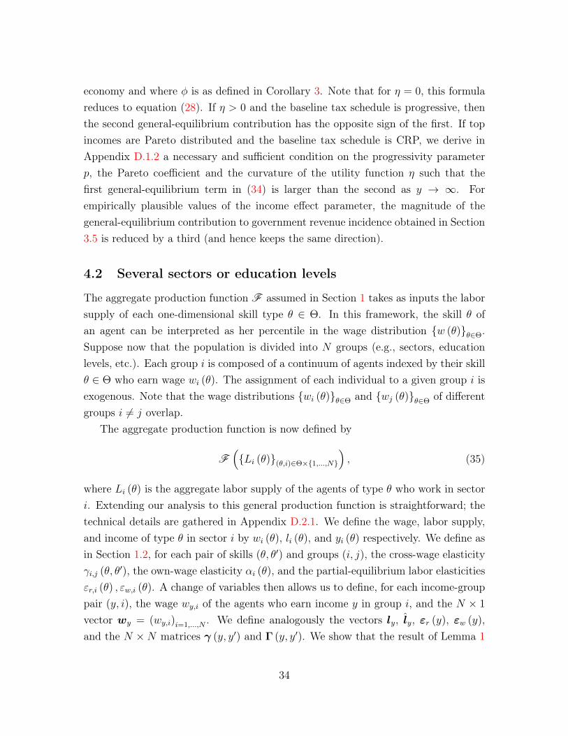
We finally extend two of the most influential results from the Mirrleesian literatureto our framework with endogenous wages. The first is the optimal top tax rateformula of Saez (2001). We derive a particularly simple closed-form generalization ofthis result in terms of one additional sufficient statistic, namely, the (finite) elasticityof substitution between skills. The second result is the familiar U-shaped pattern ofoptimal marginal tax rates first obtained by Diamond (1998). The general equilibriumforces not only confirm this pattern, but make it even more pronounced, with astronger dip in the bulk of the income distribution. We provide an economic intuitionfor this more pronounced U-shape that is based on the same economic reasoning thanour results on the incidence of tax reforms. Thus, besides the study of the incidenceof reforms of the current tax system, our tax reform approach also complements themechanism-design approach to optimal taxation in general equilibrium by providing aclearer economic understanding of the optimality conditions. Numerical simulationsconfirm these insights. Moreover, when the production function is Translog and theelasticity of substitution is distance-dependent, the optimal tax schedule is very closeto the Cobb-Douglas limit.

4

Related Literature. This paper is related to the literature on tax incidence (see,e.g., Harberger (1962) and Shoven and Whalley (1984) for the seminal papers, Hines(2009) for emphasizing the importance of general equilibrium in taxation, and Kot-likoff and Summers (1987) and Fullerton and Metcalf (2002)) for comprehensive sur-veys. Our paper extends this framework to an economy with a continuum of (labor)inputs with arbitrary nonlinear tax schedules, i.e., we study tax incidence in theworkhorse model of optimal nonlinear labor income taxation of (Mirrlees, 1971; Dia-mond, 1998).

The optimal taxation problem in general equilibrium with arbitrary nonlinear taxinstruments has originally been studied by Stiglitz (1982) in a model with two types.The key result of Stiglitz (1982) is that at the optimum tax system, general equilib-rium forces lead to a more regressive tax schedule. In the recent optimal taxationliterature, there are two strands that relate to our work. First, a series of importantcontributions by Scheuer (2014); Rothschild and Scheuer (2013, 2014); Scheuer andWerning (2017), Chen and Rothschild (2015), Ales, Kurnaz, and Sleet (2015), Alesand Sleet (2016), and Ales, Bellofatto, and Wang (2017) form the modern analysis ofoptimal nonlinear taxes in general equilibrium.2 Specifically, Rothschild and Scheuer(2013, 2014) generalize Stiglitz (1982) to a setting with N sectors and a continuum of(infinitely substitutable) skills in each sector, leading to a multidimensional screeningproblem. Ales, Kurnaz, and Sleet (2015) and Ales and Sleet (2016) microfound theproduction function by incorporating an assignment model into the Mirrlees frame-work and study the implications of technological change and CEO-firm matching foroptimal taxation. Our baseline model is simpler than those of Rothschild and Scheuer(2013, 2014) and Ales, Kurnaz, and Sleet (2015). In particular, different types earndifferent wages (there is no overlap in the wage distributions of different types, as op-posed to the framework of Rothschild and Scheuer (2013, 2014)), and the productionfunction is exogenous (in contrast to Ales, Kurnaz, and Sleet (2015)).3 The generaldistinction is that these papers focus on optimal taxation by applying the methodsof mechanism design, whereas our use of the variational approach and integral equa-

2Rothstein (2010) studies the desirability of EITC-type tax reforms in a model with heterogenouslabor inputs and nonlinear taxation. He only considers own-wage effects, however, and no cross-wage effects. Further he treats intensive margin labor supply responses as occurring along linearizedbudget constraints.

3Finally, our setting is distinct from those of Scheuer and Werning (2016, 2017), whose modelingof the technology is such that the general equilibrium effects cancel out at the optimum tax schedule,so that the formula of Mirrlees (1971) extends to their general production functions. We discuss indetail the difference between our framework and theirs in Appendix A.2.4 .

5

tions allow us to study more generally the incidence of reforming in any direction anarbitrary tax system – as we show, the (possibly suboptimal) tax system to whichthe reform is applied is a crucial determinant of the direction and size of the generalequilibrium effects. Moreover, for optimal income taxes, our setting and methods al-low us to get sharper and novel characterizations: transparent optimum tax formula,closed-form expression for the top tax rate, generalization of the U-shape of the opti-mal marginal tax rates. Note finally that we also analyze an extension of our baselineframework to production functions that allow for overlapping wage distribution inSection 4.2.

Our modeling of the production function is motived by an empirical literaturethat estimates the impact of immigration on the native wage distribution and groupsworkers according to their position in the wage distribution (Card (1990), Borjaset al. (1997), Dustmann, Frattini, and Preston (2013)). The empirical literature onimmigration is a useful benchmark because it studies the impact of labor supplyshocks of certain skills on relative wages, which is exactly the channel we want toanalyze in our tax setting (except that in our model the labor supply shocks areinduced by tax reforms). An alternative in the immigration literature is to groupworkers by education levels (Borjas, 2003; Card, 2009). We fully extend our analysisand results to a production function with different education groups in Section 4.2.

Our study of tax incidence is based on a variational, or “tax reform” approach,originally pioneered by Piketty (1997), Saez (2001, 2002), and extended to severalother contexts by, e.g., Kleven, Kreiner, and Saez (2009) and Golosov, Tsyvinski, andWerquin (2014). In this paper we extend this approach to the general equilibriumframework with endogenous wages. We derive a parsimonious and intuitive extensionof the Diamond (1998) formula for optimal marginal tax rates in terms of sufficientstatistics, and show that the general-equilibrium correction to the optimum is U-shaped. We then derive a closed-form expression for the optimal top tax rate andthereby extend that of Saez (2001) to endogenous wages.4

Finally, our paper is related to the literature that characterizes optimal govern-ment policy, within restricted classes of nonlinear tax schedules, in general equilibriumextensions of the continuous-type Mirrleesian framework. Heathcote, Storesletten,

4Our generalization of the optimal top tax rate to the case of endogenous wages is related toPiketty, Saez, and Stantcheva (2014), who extend the Saez (2001) top tax formula to a setting witha compensation bargaining channel using a variational approach. More generally, Rothschild andScheuer (2016) study optimal taxation in the presence of rent-seeking. In this paper we abstractfrom such considerations and assume that individuals are paid their marginal productivity.

6

and Violante (2016) study optimal tax progressivity in a model where agents faceidiosyncratic risk and can invest in their skills. Itskhoki (2008) and Antras, de Gor-tari, and Itskhoki (2016) characterize the impact of distortionary redistribution ofthe gains from trade in an open economy. Their production functions are CES witha continuum of skills and restrict the tax schedule to be of the CRP functional form.On the one hand, our model is simpler than their framework as we study a static andclosed economy with exogenous skills. On the other hand, for most of our theoreticalanalysis we do not restrict ourselves to a particular functional form for taxes northe production function. Our papers share, however, one important goal: to derivesimple closed form expressions for the effects of tax reforms in general-equilibriumMirrleesian environments.

This paper is organized as follows. Section 1 describes our framework and definesthe key structural elasticity variables. In Section 2 we analyze the tax incidence prob-lem with a continuum of wages and nonlinear income taxes, focusing on the impactof tax reforms on individual variables (labor supply, wages, utilities). In Section 2we derive the incidence of taxes on aggregate variables (government revenue, socialwelfare). In Section 4 we explore various generalizations of our baseline environment.Finally, in Section 5 we derive optimal taxes in general equilibrium. The proofs of allthe formulas and results of this paper are gathered in the Appendix.

1 The baseline environment

1.1 Preferences, technology and equilibrium

Individual behavior

In the simplest version of our model, individuals have a quasilinear utility functionover consumption c and labor supply l given by c� v (l), where the disutility of laborv : R+ ! R+ is twice continuously differentiable, strictly increasing, and strictlyconvex.

There is a continuum of skills ✓ 2 ⇥ = [✓, ¯✓] ⇢ R+, distributed according to thecontinuous p.d.f. f (·) and c.d.f. F (·). An individual with skill ✓ earns a wage w(✓)

that she takes as given. She chooses her labor supply l(✓) and earns taxable incomey(✓) = w(✓)l(✓). Her consumption is equal to y (✓) � T (y (✓)), where T : R+ ! R

7

is a twice continuously differentiable income tax schedule. The optimal labor supplychoice l (✓) satisfies the first-order condition of the utility-maximization problem:5

v0 (l (✓)) = [1� T 0(w (✓) l (✓))]w (✓) . (1)

We denote by U (✓) the agent’s indirect utility and by L (✓) ⌘ l (✓) f (✓) the totalamount of labor supplied by individuals of type ✓.

Remark. Without loss of generality, we can assume that wages w (✓) are strictlyincreasing in the types ✓. In other words, one can interpret each ✓ as a given skillinvolved in production, and order these skills by their wage, given the tax schedule T .In particular, we can normalize ⇥ = [0, 1] with a distribution f (✓) that is uniform, sothat ✓ indexes the agent’s percentile in the wage distribution.6 We show in AppendixA.2.3 that, by the Spence-Mirrlees condition, the pre-tax income function ✓ 7! y (✓)

is then also strictly increasing. There is therefore a one-to-one map between skills ✓(or wages w (✓)) and pre-tax incomes y(✓).7 We denote by fY (y(✓)) = (y0(✓))�1 f(✓)

the density of incomes and by FY (·) the corresponding c.d.f. in the economy.

Production and wages

There is a continuum of mass 1 of identical firms that produce output using the laborof all skills ✓. We represent the continuum of labor inputs L = {L (✓)}✓2⇥ as a finite,non-negative measure on the compact metric space (⇥,B (⇥)).8 We then define theproduction function as F (L ) = F ({L (✓)}✓2⇥) and write the representative firm’s

5Note that the dependence of labor supply on the initial tax schedule T is left implicit forsimplicity. Whenever necessary, we denote the solution to (1) by l (✓;T ).

6In Section 4.2, we relax the assumption that all agents assigned to a given skill ✓ earn the samewage w (✓).

7If the tax system changes, generally, the ordering of wages may change (see Section 3.4 fordetails). Our analysis does not require that the initial ordering remains unaffected by the taxreforms we consider.

8Thus, for any Borelian set B 2 B (⇥) (e.g., an interval in ⇥), L (B) is the total amount oflabor supplied by individuals with productivity ✓ 2 B. This construction follows Hart (1979) andFradera (1986).

8

profit-maximization problem given the wage schedule {w (✓)}✓2⇥ as9

maxL

F (L )�ˆ⇥

w (✓)L (✓) d✓

�

.

We assume that the production function F has constant returns to scale. In equilib-rium, firms earn no profits and the wage w (✓) is equal to the marginal productivityof type-✓ labor, that is,10

w (✓) =@

@L (✓)F (L ) . (2)

A commonly used production function, which we use for some of our results, isthe CES technology.

Example 1. (CES technology.) The production function has a constant elasticityof substitution (CES) if

F (L ) =

ˆ⇥

a (✓) (L (✓))��1� d✓

�

��1

, (3)

for some constant � 2 [0,1) and parameters a (✓) 2 R+. The wage schedule isgiven by w (✓) = a (✓) (L (✓) /F (L ))

�1/�. The cases � = 1 and � = 0 correspondrespectively to the Cobb-Douglas and Leontieff production functions, and � = 1implies that wages are exogenous.

Government

Government revenue is given by

R =

ˆ⇥

T (y(✓))f(✓)d✓. (4)

9Note that an alternative interpretation of our framework is that different types of workersproduce different types of goods that are imperfect substitutes in household consumption. See, e.g.,Acemoglu and Autor (2011).

10Equation (2) ignores the technical difficulties involved with the fact that F has continuum ofarguments. Formally, w (✓) is equal to the Gateaux derivative of the production function when thelabor effort schedule L is perturbed in the direction of the Dirac measure at ✓, that is, w (✓) =

lim

µ!0

1µ {F (L + µ�✓)� F (L )}.

9

We denote the local rate of progressivity of the tax schedule T by

p (y) ⌘ �@ ln [1� T 0(y)]

@ ln y=

yT 00(y)

1� T 0(y)

.

It is equal to (minus) the elasticity of the retention rate 1 � T 0(y) with respect to

income y.

Example 2. (CRP tax schedule.) The tax schedule has a constant rate of pro-gressivity (CRP) if T (y) = y� 1�m

1�py1�p, for p < 1.11 This tax schedule is linear (resp.,

progressive, regressive), i.e., the marginal tax rates T 0(y) and the average tax rates

T (y) /y are constant (resp., increasing, decreasing), if p = 0 (resp., p > 0, p < 0).

The government evaluates social welfare by means of a Bergson-Samuelson concavesocial welfare function G : R ! R. Denote by � the marginal value of public funds.12

We then define social welfare, expressed in monetary units, by:

W ⌘ R +

1

�

ˆ⇥

G [y (✓)� T (y (✓))� v (l (✓))] f (✓) d✓. (5)

We denote by g (✓), or equivalently g (y (✓)), the social marginal welfare weight13

associated with individuals of type ✓ as

g (✓) =1

�G0

[y (✓)� T (y (✓))� v (l (✓))] .

The weight g (✓) is the social value of giving one additional unit of consumption toindividuals with type ✓, relative to distributing it uniformly in the whole population.

1.2 Elasticity concepts

We now introduce notations for the elasticities that we use in our incidence andoptimal tax formulas. All of them are structural parameters that are known in closed-form.

11See, e.g., Musgrave and Thin (1948); Bénabou (2002); Heathcote, Storesletten, and Violante(2016).

12The marginal value of public funds � is determined by imposing that all of the perturbations ofthe tax system that we consider are revenue-neutral, that is, by redistributing (or taxing) lump-sumany excess revenue. Thus � is the social value of distributing an additional unit of revenue uniformlyin the entire population. In the optimal taxation problem that we study in Sections 3.4 and 5, � isnaturally the Lagrange multiplier on the government budget constraint.

13See, e.g., Saez and Stantcheva (2016).

10

Labor supply elasticities

We define the elasticity of labor supply of skill type ✓ with respect to the retentionrate r (✓) ⌘ 1� T 0

(y (✓)) as14

"Sr (✓) =@ ln l (✓)

@ ln r (✓)=

e (✓)

1 + p (y (✓)) e (✓), (6)

where e (✓) = v0(l(✓))l(✓)v00(l(✓)) and the superscript S stands for (labor) supply. This elasticity

differs from the more standard variable e (✓) as it accounts for the fact that if the taxschedule is nonlinear, a change in individual labor supply l (✓) induces endogenouslya change in the marginal tax rate T 0

(y (✓)) (given by the rate of progressivity p (y (✓))

of the tax schedule), and hence a further labor supply adjustment e (✓). Solving forthis fixed point leads to the correction term p (y (✓)) e (✓) in the denominator of (6).15

For further details see Appendix A.1.We also define the elasticity of labor supply of type ✓ with respect to the wage

w (✓) as

"Sw (✓) =@ ln l (✓)

@ lnw (✓)= (1� p (y (✓))) "Sr (✓) . (7)

This elasticity differs from (6) because a wage change affects (1� T 0(y (✓)))w (✓)

both directly as in the case of an exogenous perturbation in the retention rate, andindirectly through its effect on the marginal tax rate T 0

(w (✓) l (✓)) if the tax scheduleis nonlinear. The latter is accounted for by the correction p (y (✓)) "Sr (✓) in (7).

Cross-wage and own-wage elasticities

We define the structural cross-elasticity of the wage of type ✓0, w (✓0), with respect tothe labor supply of type ✓ 6= ✓0, L (✓), as:16,17

� (✓0, ✓) =@ lnw (✓0)

@ lnL (✓)=

L (✓)F 00✓0,✓

F 0✓0

, (8)

14Since there is a one-to-one map between types ✓ and incomes y (✓), we can write interchangeably"Sr (✓) or "Sr (y (✓)), and similarly for the elasticities "Sw (✓) and ↵ (✓) defined below.

15See also Jacquet and Lehmann (2017) and Scheuer and Werning (2017).16We assume that ✓0 7! � (✓0, ✓) is a continuous map on ⇥ \ {✓}.17The natural change of variables between types ✓ and incomes y (✓) for the cross-wage elasticities

reads �(y(✓1), y(✓2)) = (y0(✓2))�1 �(✓1, ✓2). See Appendix A.2 for details.

11

where F 0✓0 and F 00

✓0,✓ denote the first and second partial derivatives of the productionfunction F with respect to the labor inputs of types ✓0 and ✓. The structural cross-wage elasticity between two skills (✓0, ✓) with ✓0 6= ✓ is non-zero if they are imperfectsubstitutes. Although this is not necessary for our theoretical analysis,18 we usuallyassume for simplicity in our discussions below that these elasticities are positive (asis always the case, for instance, if the production function is CES), i.e., that any twoskills ✓0 6= ✓ are Edgeworth complements in production.

The function ✓0 7! @ lnw(✓0)@ lnL(✓) is generally discontinuous at ✓0 = ✓, i.e., when we con-

sider the impact of the labor of type-✓ agents on their own wage. We call own-wageelasticity ↵ (✓) the difference between @ lnw(✓)

@ lnL(✓) and lim✓0!✓ � (✓0, ✓). By subtracting

from @ lnw(✓)@ lnL(✓) the complementarity lim✓0!✓ � (✓

0, ✓) between the skill ✓ and its neigh-boring skills ✓0 ⇡ ✓, the variable ↵ (✓) captures the impact of the labor effort L (✓)

on the wage w (✓) arising purely from the fact that the marginal productivity of skill✓ is a non-constant (say, decreasing) function of the aggregate labor of its own type.Formally, we define

↵ (✓) = �

@ lnw (✓)

@ lnL (✓)� lim

✓0!✓

@ lnw (✓0)

@ lnL (✓)

�

= �

L (✓)F 00✓,✓

F 0✓

� lim

✓0!✓

L (✓)F 00✓0,✓

F 0✓0

�

. (9)

This elasticity is positive if the marginal productivity of the labor input L (✓) isdecreasing. Although this is not required for our theoretical analysis, we assume forsimplicity in our discussions below that this is the case for all skills ✓.19

Example. (CES technology.) In the case of a CES production function, the cross-wage elasticities are given by � (✓0, ✓) = 1

�a (✓) (L (✓) /F (L ))

��1� and the own-wage

elasticities are given by ↵ (✓) = 1/� for all ✓0, ✓. Note that ↵ (✓) > 0 is constant andthat � (✓0, ✓) > 0 does not depend on ✓0, implying that a change in the labor supplyof type ✓ has the same effect, in percentage terms, on the wage of every type ✓0 6= ✓.Denoting by � (✓0, ✓) = �

h

@ ln(w(✓0)/w(✓))@ ln(L(✓0)/L(✓))

i�1

the elasticity of substitution between anytwo labor inputs, we have � (✓0, ✓) = � for all (✓0, ✓) 2 ⇥

2.

18For instance, a Translog production function can allow for negative cross-wage elasticities.Negative cross-input effects arise, for instance, in the capital-skill complementarity literature (seeKrusell et al. (2000)).

19The variable ↵ (✓) can also be interpreted as the inverse of the partial-equilibrium elasticity1/"Dw (✓) of labor demand of type ✓ with respect to the wage w (✓).

12

Elasticities of equilibrium labor

We define the elasticities of labor of type ✓ in partial equilibrium, i.e., keeping theprices w (✓0) and quantities L (✓0) constant in all other “markets” ✓0 6= ✓, by

"r (✓) ="Sr (✓)

1 + ↵ (✓) "Sw (✓), and "w (✓) =

"Sw (✓)

1 + ↵ (✓) "Sw (✓). (10)

Intuitively, a percentage increase in the labor supply of type-✓ individuals by "Sr (✓)

or "Sw (✓), caused by an increase in their retention rate or their wage, lowers their ownwage (due to the decreasing marginal productivity) by ↵ (✓), which in turn dampensthe initial increase in their labor supply by ↵ (✓) "Sw (✓). Solving for the fixed pointleads to expressions (10).20

2 Tax incidence

Consider a given initial, potentially suboptimal, tax schedule T , e.g., the U.S. taxcode. In this section we derive closed-form formulas for the first-order effects ofarbitrary local perturbations (“tax reforms”) of this tax schedule on individual laborsupplies, wages and indirect utilities.

2.1 Incidence of tax reforms on labor supply

As in the case of exogenous wages (Saez, 2001), analyzing the incidence of tax reformsrelies crucially on solving for each individual’s change in labor supply in terms ofbehavioral elasticities. This problem is, however, much more involved in generalequilibrium. In the setting with exogenous wages, in the absence of income effects,a change in the tax rate of a given individual, say ✓, induces only a change in thelabor effort of that agent (measured by the elasticity (6)). In the general equilibriumsetting, instead, this labor supply response of type ✓ affects the wage, and hence thelabor supply, of every other skill ✓0 6= ✓. This in turn feeds back into the wage of✓, which further impacts labor supplies, and so on. Representing the total effect of

20Interpreting ↵ (✓) = 1/"Dw (✓) as the inverse of the labor demand elasticity with respect to thewage, we can write 1

"w(✓) =1

"Sw(✓)+1

"Dw (✓) . As expected from from the Ramsey tax literature (see, e.g.,Stiglitz (2015)), this sum of inverse elasticities of labor supply and labor demand is an importantvariable for our tax incidence analysis.

13

this infinite sequence caused by arbitrarily non-linear tax reforms is thus a priori acomplex task.21

The key step towards the general characterization of the economic incidence oftaxes, and our first main theoretical contribution, consists of showing that this prob-lem can be mathematically formulated as solving an integral equation (Lemma 1).22

We can thus apply the tools and results of the theory of integral equations to solvein closed-form for the labor supply adjustments in general equilibrium (Proposition1). The incidence on wages and utilities is then straightforward to derive (Sections2.2 and 2.3).

Formally, consider an arbitrary non-linear reform of the initial tax schedule T (·).This tax reform can be represented by a continuously differentiable function ⌧ (·) onR+, so that the perturbed tax schedule is T (·)+µ⌧ (·), where µ 2 R parametrizes thesize of the reform. Our aim is to compute the first-order effect of this perturbationon individual labor supply (i.e., the solution to the first-order condition (1)), whenthe magnitude of the tax change is small, i.e., as µ ! 0. This is formally expressedby the Gateaux derivative of the labor supply functional T 7! l (✓;T ) in the direction⌧ , that is,23

dl (✓) ⌘ lim

µ!0

1

µ

⇥

l(✓;T + µ⌧)� l (✓;T )⇤

, and ˆl (✓) ⌘ dl (✓)

l (✓;T ).

The variable dl (✓) (resp., ˆl (✓)) gives the absolute (resp., percentage) change in thelabor supply of type ✓ in response to the tax reform ⌧ , taking into account all of thegeneral equilibrium effects induced by the endogeneity of wages. We define anal-ogously the absolute changes in individual wages dw (✓), indirect utilities du (✓),government revenue dR and social welfare dW , and the corresponding percentagechanges w (✓), u (✓), ˆR, ˆW .

21We can always define, for each specific tax reform one might consider implementing, a “policyelasticity” (as in, e.g., Hendren (2015), Piketty and Saez (2013)), equal to each individual’s totallabor supply response to the corresponding reform. However the key challenge of the incidenceproblem consists of expressing this total labor supply response in terms of the structural elasticityparameters introduced in Section 1.2.

22The general theory of linear integral equations is exposed in, e.g., Tricomi (1985), Kress (2014),and, as a concise introduction, in Zemyan (2012). Moreover, closed-form solutions can be derived inmany cases (see Polyanin and Manzhirov (2008)). Finally, numerical techniques are widely availableand can be easily implemented (see, e.g., Press (2007) and Section 2.6 in Zemyan (2012)), leading tostraightforward quantitative evaluations of the incidence of arbitrary tax reforms (see Section 3.5).

23The notations dl (✓) and ˆl (✓) ignore for simplicity the dependence of these derivatives on theinitial tax schedule T and on the tax reform ⌧ .

14

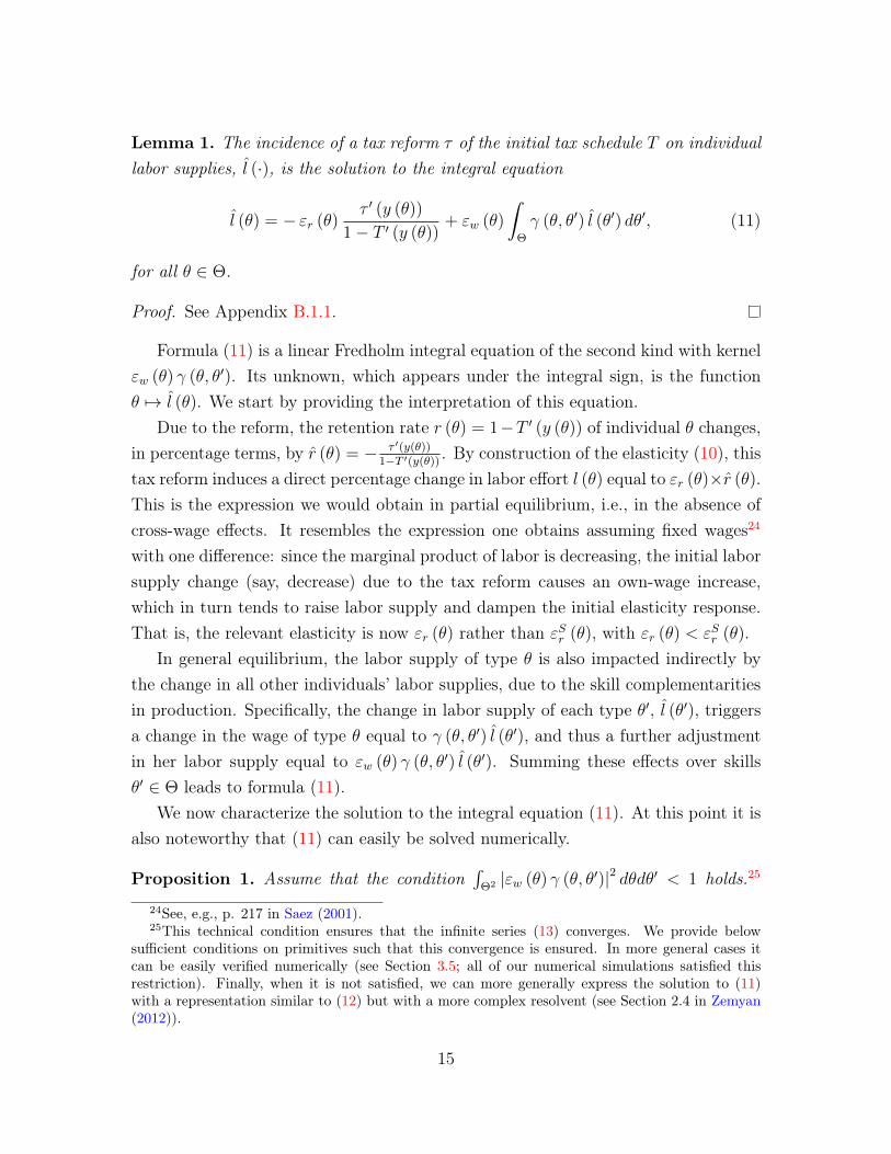
Lemma 1. The incidence of a tax reform ⌧ of the initial tax schedule T on individuallabor supplies, ˆl (·), is the solution to the integral equation

ˆl (✓) = � "r (✓)⌧ 0 (y (✓))

1� T 0(y (✓))

+ "w (✓)

ˆ⇥

� (✓, ✓0) ˆl (✓0) d✓0, (11)

for all ✓ 2 ⇥.

Proof. See Appendix B.1.1.

Formula (11) is a linear Fredholm integral equation of the second kind with kernel"w (✓) � (✓, ✓0). Its unknown, which appears under the integral sign, is the function✓ 7! ˆl (✓). We start by providing the interpretation of this equation.

Due to the reform, the retention rate r (✓) = 1�T 0(y (✓)) of individual ✓ changes,

in percentage terms, by r (✓) = � ⌧ 0(y(✓))1�T 0(y(✓)) . By construction of the elasticity (10), this

tax reform induces a direct percentage change in labor effort l (✓) equal to "r (✓)⇥r (✓).This is the expression we would obtain in partial equilibrium, i.e., in the absence ofcross-wage effects. It resembles the expression one obtains assuming fixed wages24

with one difference: since the marginal product of labor is decreasing, the initial laborsupply change (say, decrease) due to the tax reform causes an own-wage increase,which in turn tends to raise labor supply and dampen the initial elasticity response.That is, the relevant elasticity is now "r (✓) rather than "Sr (✓), with "r (✓) < "Sr (✓).

In general equilibrium, the labor supply of type ✓ is also impacted indirectly bythe change in all other individuals’ labor supplies, due to the skill complementaritiesin production. Specifically, the change in labor supply of each type ✓0, ˆl (✓0), triggersa change in the wage of type ✓ equal to � (✓, ✓0) ˆl (✓0), and thus a further adjustmentin her labor supply equal to "w (✓) � (✓, ✓0) ˆl (✓0). Summing these effects over skills✓0 2 ⇥ leads to formula (11).

We now characterize the solution to the integral equation (11). At this point it isalso noteworthy that (11) can easily be solved numerically.

Proposition 1. Assume that the condition´⇥2 |"w (✓) � (✓, ✓0)|2 d✓d✓0 < 1 holds.25

24See, e.g., p. 217 in Saez (2001).25This technical condition ensures that the infinite series (13) converges. We provide below

sufficient conditions on primitives such that this convergence is ensured. In more general cases itcan be easily verified numerically (see Section 3.5; all of our numerical simulations satisfied thisrestriction). Finally, when it is not satisfied, we can more generally express the solution to (11)with a representation similar to (12) but with a more complex resolvent (see Section 2.4 in Zemyan(2012)).

15

The unique solution to the integral equation (11) is given by

ˆl (✓) = � "r (✓)⌧ 0 (y (✓))

1� T 0(y (✓))

� "w (✓)

ˆ⇥

� (✓, ✓0) "r (✓0)

⌧ 0 (y (✓0))

1� T 0(y (✓0))

d✓0, (12)

where for all (✓, ✓0) 2 ⇥

2, the resolvent � (✓, ✓0) is defined by

� (✓, ✓0) ⌘1X

n=1

�n (✓, ✓0) , (13)

with �1 (✓, ✓0) = � (✓, ✓0) and for all n � 2,

�n (✓, ✓0) =

ˆ⇥

�n�1 (✓, ✓00) "w (✓00) � (✓00, ✓0) d✓00.

We call � (✓, ✓0) the general-equilibrium (GE) cross-wage elasticity (as opposed to thestructural cross-wage elasticity � (✓, ✓0)).


The mathematical representation (12) of the solution to the integral equation(11) has a clear economic interpretation. The first term on the right hand side of(12), �"r (✓) ⌧ 0(y(✓))

1�T 0(y(✓)) , is the partial-equilibrium effect of the reform on labor sup-ply l (✓), as already described in equation (11). The second (integral) term accountsfor the cross-wage effects in general equilibrium. Note that this integral term hasthe same structure (and interpretation) as in formula (11), except that: (i) the un-known labor supply changes ˆl (✓0), that had to be solved for, are now replaced bytheir partial-equilibrium values �"r (✓0) ⌧ 0(y(✓0))

1�T 0(y(✓0)) ; and (ii) the structural cross-wageelasticity � (✓, ✓0) is replaced by the GE cross-wage elasticity � (✓, ✓0). As we describein the next paragraph, this elasticity, defined by the series (13), expresses the totaleffect of the labor supply of type ✓0 on the wage of type ✓, i.e., it accounts for the in-finite sequence of general equilibrium adjustments induced by the complementaritiesin production.

We now interpret the definition (13) of the GE cross-wage elasticity � (✓, ✓0). Thefirst iterated kernel (n = 1) in the series (13) is simply �1 (✓, ✓

0) = � (✓, ✓0). It thus

accounts for the impact of the labor supply of type ✓0 on the wage of type ✓ throughdirect cross-wage effects. The second iterated kernel (n = 2) in (13) accounts for theimpact of the labor supply of ✓0 on the wage of ✓, indirectly through the behavior of

16

third parties ✓00. This term reads

�2 (✓, ✓0) =

ˆ⇥

� (✓, ✓00) "w (✓00) � (✓00, ✓0) d✓00. (14)

For any ✓0, a percentage change in the labor supply of ✓0 induces a percentage change inthe wage of any other type ✓00 by � (✓00, ✓0) (by definition (8)), and hence a percentagechange in the labor supply of ✓00 given by "w (✓00) � (✓00, ✓0) (by definition (10)). Thisin turn affects the wage of type ✓ by the amount � (✓, ✓00) "w (✓00) � (✓00, ✓0). Summingover all intermediate types ✓00 leads to expression (14). An inductive reasoning showssimilarly that the terms n � 3 in the resolvent series (13) account for the impactof the labor supply of ✓0 on the wage of ✓ through n successive stages of cross-wageeffects, e.g., for n = 3, ✓0 ! ✓00 ! ✓000 ! ✓.

Example. (CES technology.) Suppose that the production function is CES. Inthis case, the GE cross-wage elasticities are given by:

� (✓, ✓0) =� (✓, ✓0)

1� 1�Ey´R+

y "w (y) fY (y) dy. (15)

That is, the total impact � (✓, ✓0) of a change in the labor supply of type ✓0 on thewage of type ✓ is proportional to the direct (structural) effect � (✓, ✓0). This is becauseeach round of cross-wage general equilibrium effects, i.e., each term in the resolventseries (13), is a fraction of the first round. This in turn follows from the fact that,with a CES technology, the cross-wage elasticity � (✓, ✓0) depends only on ✓0 and isindependent of ✓, that is, a change in the aggregate labor supply of type ✓0 inducesthe same percentage adjustment in the wage of every skill ✓ 6= ✓0. Mathematically, thekernel "w (✓) � (✓, ✓0) of the integral equation (11) is then multiplicatively separablebetween ✓ and ✓0, which makes it straightforward to solve (see Appendix B.1.3 fordetails).

Sufficient conditions on primitives ensuring convergence of the resolvent

Suppose that the production function is CES with parameter � > 0, that the initialtax schedule is CRP with parameter p < 1, and that the disutility of labor is isoe-lastic with parameter e > 0. We show in Appendix A.2.1 that we have in this case1

�EyE [y"w (y)] < 1 so that, by formula (15), � (✓, ✓0) < 1. The convergence of theresolvent series (13) is thus satisfied.

17

2.2 Incidence of tax reforms on wages

Once the labor supply response ˆl (✓) is characterized in closed-form (Proposition 1),we can easily derive the incidence of an arbitrary tax reform ⌧ on individual wages.We show in Appendix B.2.1 that, for all ✓ 2 ⇥,

w (✓) =1

"Sw (✓)

"Sr (✓)⌧ 0 (y (✓))

1� T 0(y (✓))

+

ˆl (✓)

�

. (16)

This equation expresses the changes in individual wages due to the tax reform ⌧ , asa function of the labor supply changes given by (12). Its interpretation is straightfor-ward. Multiplying both sides of (16) by "Sw (✓) simply gives the adjustment of type-✓labor supply, ˆl (✓), as the sum of its response in the case of exogenous wages, �"Sr ⌧ 0

1�T 0 ,and the general equilibrium effect induced by the wage change, "Sw ⇥ w.

2.3 Incidence of tax reforms on individual welfare

Finally, we can easily derive the incidence of an arbitrary tax reform ⌧ of the initialtax schedule T on individual indirect utilities. We show in Appendix B.2.2 that

du (✓) =� ⌧ (y (✓)) + (1� T 0(y (✓))) y (✓) w (✓) , (17)

for all ✓ 2 ⇥. The first term on the right hand side of equation (17), �⌧ (y (✓)), is dueto the fact that a higher tax payment makes the individual poorer and hence reducesher utility. The second term accounts for the change in net income due to the wageadjustment w (✓).

If wages were exogenous (i.e., w (✓) = 0 in (17)), the welfare of agent ✓ wouldrespond one-for-one to the change in her total tax bill, ⌧ (y (✓)). In particular, thechange in the marginal tax rate that the reform induces, ⌧ 0 (y (✓)), would not affecther utility. This is a direct consequence of the envelope theorem: the marginal taxrate affects utility only to the extent that it leads to adjustments in labor supply(equation (1)); but labor supply is initially chosen optimally, hence a change in themarginal tax rate has only a second-order effect on welfare (conditional on a givenabsolute tax change).

In general equilibrium, however, this is no longer true, because labor supplychanges also imply movements in wages, which have first-order effects on welfare.Therefore the change in the marginal tax rate impacts individual utilities, even con-

18

ditional on a given absolute tax change. Specifically, we show:

Corollary 1. Assume that the cross-wage elasticities satisfy � (✓0, ✓) � 0 for all ✓0, ✓.For a given absolute tax change ⌧ (y (✓)) at income y (✓), an increase in the marginaltax rate ⌧ 0 (y (✓)) > 0 raises the utility of agents with type ✓ and lowers that of allother agents, i.e., du (✓) > 0, and du (✓0) < 0 for all ✓0 6= ✓.


Intuitively, a higher marginal tax rate for individuals of type ✓ makes them workless, because of the standard substitution effect, and earn more per hour worked,because of the decreasing marginal product of labor, which makes them better off. Ifthe cross-wage elasticities are positive (as is the case, for instance, if the productionfunction is CES), then the wages, and hence utilities, of all other types go down asa consequence of the lower labor effort of type ✓.26 As we show in Section 5, thisinsight generalizes that of Stiglitz (1982) and is a crucial determinant of the structureof optimal marginal tax rates.

3 Aggregate effects of tax reforms

Having derived the change in the equilibrium amount of labor (12) and the changein wages (16) in response to a tax reform ⌧ , the incidence on government revenue R,defined in (4), directly follows:

dR =

ˆR+

⌧ (y) fY (y) dy +

ˆR+

T 0(y)

⇥

ˆl (y) + w (y)⇤

yfY (y) dy, (18)

where ˆl (y) ⌘ ˆl(✓y) and w (y) ⌘ w(✓y) are the labor supply and the wage changes ofagents with income y (and type ✓y). The first term on the right hand side of (18) isthe mechanical effect of the tax reform ⌧ (·), i.e., the change in government revenueif the individual behavior and her wage remained constant. The second term is thebehavioral effect of the reform. The labor supply and wage adjustments ˆl (y) andw (y) both induce a change in government revenue proportional to the marginal tax

26Note that an increase in the marginal tax rate at income y (✓) implies in particular that indi-viduals with skill ✓0 > ✓ are made worse off for two separate reasons: (i) their total tax bill is nowmechanically higher, since the marginal tax rate on income y (✓) has increased; (ii) their wage islower, since the labor supply of agents ✓ is distorted downward.

19

rate T 0(y). Summing these effects over all individuals using the density of incomes

fY (y) yields (18).In this section we derive the economic implications of formula (18). Sections

3.1 and 3.2 contain useful preliminary steps. Section 3.3 contains our main results.Section 3.4 extends the results of this section to a general social welfare objective andderives as a by-product a characterization of the optimal tax schedule.

Elementary tax reforms

From now on, we focus on a specific class of “elementary” tax reforms, represented bythe step function ⌧ (y) = (1� FY (y⇤))�1 I{y�y⇤} for a given income level y⇤.27 Thatis, the total tax liability increases by the constant amount (1� FY (y⇤))�1 aboveincome y⇤, and the marginal tax rates are perturbed by the Dirac delta functionat y⇤, ⌧ 0 (y) = (1� FY (y⇤))�1 �y⇤ (y). Intuitively, this reform consists of raising themarginal tax rate at only one income level y⇤ 2 R+, which implies a uniform lump-sumincrease in the total tax payment of agents with income y > y⇤. The normalizationby (1� FY (y⇤))�1 implies that the statutory increase in government revenue due tothe reform (i.e., the first term in the right hand side of (18), which ignores the agents’behavioral responses) is equal to $1.28 We denote by dR (y⇤) the total effect ongovernment revenue (18) of the elementary tax reform at income y⇤.

Finally, note that any other tax reform can be expressed as a weighted sum of suchincome-specific perturbations.29 Specifically, the effect of an arbitrary tax reform ⌧

on government revenue is given by

dR (⌧) =

ˆR+

dR (y⇤) (1� FY (y⇤)) ⌧ 0 (y⇤) dy⇤. (19)

The focus on the elementary tax reforms at arbitrary income levels is thus without27Note that the function I{y�y⇤} is not differentiable. We show in Appendix C.1 that we can

nevertheless use our theory to analyze this reform by applying (12) to a sequence of smooth per-turbations {⌧ 0n (y)}n�1 that converges to the Dirac delta function �y⇤

(y). This notation simplifiesthe exposition and is made only for convenience. All of our formulas can be easily written for anysmooth tax reform ⌧ rather than the step functions (see formula (19)).

28Heuristically, consider a perturbation that raises the marginal tax rate by dT 0 on a small incomeinterval [y⇤ � dy, y⇤], so that the total tax payment above income y⇤ raises by the amount dT 0 ⇥ dyequal to, say, $1. This class of tax reforms has been introduced by Saez (2001). Then shrink the sizeof the income interval on which the tax rate is increased, i.e. dy ! 0, while keeping the increase inthe tax payment above y⇤ fixed at $1. The limit of the marginal tax rate increase dT 0 is the Diracmeasure at y⇤, and the change in the total tax bill converges to its c.d.f., the step function I{y�y⇤}.

29See Golosov, Tsyvinski, and Werquin (2014) for details.

20

loss of generality.

3.1 Comparison to the exogenous-wage benchmark

Most of the taxation literature assumes exogenous wages. In this case, the incidenceon government revenue is given by expression (18) with w (y) ⌘ w

ex

(y) = 0 andˆl (y) ⌘ ˆl

ex

(y) = �"Sr (y)⌧ 0(y)

1�T 0(y) . Applying this formula to the elementary tax reformat income y⇤ leads to

dRex

(y⇤) = 1� "Sr (y⇤)

T 0(y⇤)

1� T 0(y⇤)

y⇤fY (y⇤)

1� FY (y⇤). (20)

Equation (20) expresses the impact of an increase in the marginal tax rate at incomey⇤ as the sum of a mechanical increase in government revenue, which is normalizedto $1 by construction, and a behavioral revenue loss equal to the product of: (i) theendogenous reduction in the labor income of agent y⇤, y⇤

1�T 0(y⇤)"Sr (y

⇤); (ii) the share

T 0(y⇤) of this income change that accrues to the government; and (iii) the hazard

rate of the income distribution, fY (y⇤)1�FY (y⇤) . The hazard rate is a cost-benefit ratio that

measures the fraction fY (y⇤) of agents whose labor supply is distorted by the reform,relative to the fraction 1� FY (y⇤) of agents whose tax bill increases lump-sum.

By contrast, in the general equilibrium environment, the labor supply responsesˆl (y) in formula (18) are equal to the sum of those obtained in the model with ex-ogenous wages, ˆl

ex

(y), and those induced by the wage adjustments, "Sw (y) w (y) (seeformula (16)). We can therefore rewrite (18), for the elementary tax reform at incomey⇤, as

dR (y⇤) = dRex

(y⇤) +

ˆR+

⇥

T 0(y)

�

1 + "Sw (y)�⇤

w (y) yfY (y) dy, (21)

where dRex

(y⇤) is given by (20). In this expression, the term T 0(y)

�

1 + "Sw (y)�

accounts for the effects of a unit change in the wage w (y) on government revenue,both directly (via the term T 0

(y)) and through the labor supply responses it induces(via the term T 0

(y) "Sw (y)). The integral term in equation (21) therefore isolates theeffects of the endogeneity of wages on government revenue, and thus allows for aclear comparison with the benchmark formula (20). The goal of the remainder of thissection is to analyze this novel term.

21

3.2 Relationship between the own- and cross-wage elasticities

Before deriving an expression for the aggregate effects of tax reforms in general equi-librium, we start by stating the following lemma, which provides two versions ofEuler’s homogeneous function theorem in our economy.

Lemma 2. The following relationship between the own-wage elasticity and the struc-tural cross-wage elasticities is satisfied: for all y⇤,

� ↵(y⇤) +

ˆR+

�(y, y⇤)yfY (y) dy = 0, (22)

where �(y, y⇤) = �(y,y⇤)y⇤fY (y⇤) . Equivalently, this can be expressed as a relationship between

the own-wage elasticity and the GE cross-wage elasticities: for all y⇤,

� ↵ (y⇤) +

ˆR+

˜

� (y, y⇤) yfY (y) dy = 0, (23)

where ˜

� (y, y⇤) =�

1 + ↵ (y) "Sw (y)��1 �(y,y⇤)

y⇤fY (y⇤) .

Proof. See Appendix A.2. Note that if the production function is CES, then �(y, y⇤) =1/(�E [y]) is constant and, if in addition the disutility of labor is isoelastic and theinitial tax schedule is CRP, then ˜

� (y, y⇤) = �(y, y⇤) = 1/(�E [y]).

To interpret these equations, consider a one percent increase in the labor supplyof agents with income y⇤, induced for instance by a lower marginal tax rate. Theirown wage decreases by ↵(y⇤) percent, while the wages of agents y 6= y⇤ increaseby �(y, y⇤) percent. Because the production function has constant returns to scale,summing these effects has no impact on aggregate income: keeping labor suppliesfixed, the income losses y⇤↵ (y⇤) of agents with skill ✓⇤ are exactly compensated inthe aggregate by the income gains y �(y, y⇤) of the other types ✓ 6= ✓⇤. This leads toequation (22). Now, these wage changes induce labor supply changes, which in turnaffect wages through further rounds of own- and cross-effects in general equilibrium.Since Euler’s homogeneous function theorem applies at every stage, the effect onaggregate income of all these wage adjustments is again equal to zero, that is,

ˆR+

l (y)⇥ dw (y) fY (y) dy =

ˆR+

y ⇥ w (y) fY (y) dy = 0. (24)

22

This equation implies that keeping labor supplies fixed at their initial level, the reshuf-fling of wages have distributional effects but keeps the economy’s aggregate outputconstant. Using formulas (12) and (16) then leads to equation (23).

Suppose now that the disutility of labor is isoelastic, and that the initial taxschedule (before the tax reform) is linear. These assumptions imply that the elasticity"Sw (y) and the marginal tax rate T 0

(y) are constant. Constrasting equations (24)(which captures the change in aggregate output coming only from the wage changes)and (21) (which depends on the change in aggregate output coming from both thelabor supply and the wage changes) immediately leads to the following corollary:

Corollary 2. Suppose that the disutility of labor is isoelastic and that the initialtax schedule is linear. Then the incidence of an arbitrary nonlinear tax reform ongovernment revenue is identical to that obtained assuming exogenous wages, i.e., forall y⇤,

dR (y⇤) = dRex

(y⇤) ,

where dRex

(y⇤) is given by (20).

Note that this result holds for any production function that has constant returns toscale. Intuitively, constant returns to scale and the constant elasticity of labor supplyimply that the income gain of skill ✓⇤ is exactly compensated in the aggregate by theincome losses of the other types ✓ 6= ✓⇤. Since initially all income levels pay the samemarginal tax rate, the government’s tax revenue gain coming from the higher incomeof skill ✓⇤ is thus exactly compensated by the tax revenue losses coming from the restof the population. Therefore the general-equilibrium contribution to the incidence ofany tax reform on government budget, i.e. the integral term in (21), is equal to zero.

In the next section, we analyze the incidence of tax reforms on government revenuein the general case where the initial tax schedule is arbitrarily nonlinear.

3.3 Effects of tax reforms on government revenue

The following proposition expresses the impact of tax reforms on government revenuein general equilibrium and compares it to the expression (20) obtained in the modelwith exogenous wages.

Proposition 2. The incidence of the elementary tax reform at income y⇤ on govern-

23

ment revenue is given by

dR (y⇤) = dRex

(y⇤) + "r (y⇤)

⌦ (y⇤)

1� T 0(y⇤)

y⇤fY (y⇤)

1� FY (y⇤), (25)

where the variable ⌦ (y⇤) is defined by

⌦ (y⇤) =

ˆR+

h

T 0(y⇤)

�

1 + "Sw (y⇤)�

� T 0(y)

�

1 + "Sw (y)�

i

˜

� (y, y⇤) yfY (y) dy. (26)

Proof. See Appendix C.2.

Before deriving the economic implications of equation (25), it is useful to firstsketch its proof. The direct effect of the elementary tax reform at income level y⇤ isto cause a decrease in the labor supply of type ✓⇤ by � y⇤"r(y⇤)

1�T 0(y⇤) . Using Proposition1, we can show that this implies (i) a positive own-wage effect on skill ✓⇤ equal to� y⇤"r(y⇤)

1�T 0(y⇤) ⇥ (�↵ (y⇤)) > 0, and (ii) a negative cross-wage effect on each skill ✓ 2 ⇥

(or income y) equal to � y⇤"r(y⇤)1�T 0(y⇤) ⇥

�(y,y⇤)1+↵(y)"Sw(y) < 0. In turn, a wage adjustment w (y)

at income y impacts government revenue by T 0(y)

�

1 + "Sw (y)�

⇥ w (y). Hence thegeneral-equilibrium contribution to the incidence of the tax reform on governmentrevenue is given by

⌦ (y⇤) = T 0(y⇤)

�

1 + "Sw (y⇤)�

↵ (y⇤)�ˆR+

T 0(y)

�

1 + "Sw (y)�

˜

� (y, y⇤) yfY (y) dy.

(27)Euler’s theorem (23) then leads to expression (26).

Suppose first that the disutility of labor is isoelastic and that the tax schedule isCRP (progressive or regressive), so that the labor supply elasticity "Sw (y) is constant.Moreover, assume in addition that the production function is CES, so that ↵ (y⇤) and˜

� (y, y⇤) are also constant. We then have

⌦ (y⇤) / T 0(y⇤)↵ (y⇤)�

ˆR+

T 0(y) ˜� (y, y⇤) yfY (y) dy

=

1

�

T 0(y⇤)�

ˆR+

T 0(y)

y

EyfY (y) dy

�

.

Suppose that the marginal tax rates are increasing in the initial economy, i.e., therate of progressivity is p > 0. Then, in response to the tax reform, the governmentrevenue gain from the higher income of agents ✓⇤, which is proportional to T 0

(y⇤), is

24

increasing in y⇤, whereas the tax revenue loss from the rest of the population, whichis proportional to �E[T 0

(y) y], is independent of y⇤. That is, the larger the incomey⇤, the higher the marginal tax rate at y⇤ relative to the (income-weighted) averagemarginal tax rate in the economy. Therefore, starting from a progressive tax schedule,the revenue gains from raising the marginal tax rates at the top and lowering them atthe bottom, i.e., from raising further the progressivity of the tax schedule, are higherin general equilibrium (⌦ (y⇤) > 0) than the standard partial-equilibrium formula(20) would predict.

More generally, for an arbitrary production function, equation (27) implies thatthe general equilibrium contribution ⌦ (y⇤) is positive (resp., negative) if the marginaltax rate at y⇤ is larger (resp., smaller) than a weighted-average marginal tax rate inthe economy, where the weights are now given by the modified cross-wage elastici-ties ˜

� (y, y⇤). Therefore, the efficiency loss from raising the tax rate at income y⇤

depends, in addition to the standard variables obtained in partial equilibrium, on theco-variation between the initial marginal tax rates T 0

(y) in the economy, and thecomplementarities �(y, y⇤) with agent y⇤ in production. This is intuitive: the incomeof every individual is affected by the tax reform; the fiscal consequences depend onthe size of these income changes (captured by the schedule of GE cross-wage elastic-ities) times the share of these changes that accrues to the government (captured bythe schedule of marginal tax rates in the economy).

We conclude this section by formally stating the result we obtained above in thespecial case of a CES production function.

Corollary 3. Suppose that the disutility of labor is isoelastic, that the initial taxschedule is CRP, and that the production function is CES. The incidence of the ele-mentary tax reform at income y⇤ on government revenue can then be written as

dR (y⇤) = dRex

(y⇤) + � "SrT 0

(y⇤)� ¯T 0

1� T 0(y⇤)

y⇤fY (y⇤)

1� FY (y⇤), (28)

where dRex

(y⇤) is given by (20), � =

1+"w�+"w

,30 and ¯T 0= E [yT 0

(y)] /Ey. Thus thegeneral-equilibrium effect on incidence is positive (resp., negative) if the marginal tax

30Recall that if the production function is CES, each round of cross-wage effects in generalequilibrium is a constant fraction of the first round, so that the GE elasticity � (y, y⇤) is propor-tional to the structural (first-round) elasticity � (y, y⇤) (equation (15)). In equation (28), the terms"Sr

T 0(y⇤)�T 0

1�T 0(y⇤)y⇤fY (y⇤)1�FY (y⇤) are those that would be obtained by ignoring the full general-equilibrium ad-

justment of wages and labor supply, and instead focusing only on the first round of wage adjustments;� is then the discount factor that accounts for the second, third, etc. rounds of general equilibrium

25

rate at y⇤ is larger (resp., smaller) than the income-weighted average marginal taxrate in the economy.


3.4 Social welfare and optimal tax schedule

The analysis of Section 3.3 can be easily extended to compute the incidence oftax reforms on social welfare, replacing dR (y⇤) with dW (y⇤) in equation (25).31

The technical details are gathered in Appendix C.4. The first difference is thatthe exogenous-wage term dR

ex

(y⇤) in the right hand side of (25) is replaced bydW

ex

(y⇤) = dRex

(y⇤)� g (y⇤), where �g (y⇤) ⌘ �E [g (y) |y � y⇤ ] is the total welfareloss from a higher marginal tax rate at income y⇤. The second difference is thatthe variable T 0

(y)�

1 + "Sw (y)�

in equation (26), which measures the total impact ofa wage adjustment w (y) on the government budget, is now replaced by the moregeneral expression

(y) =�

1 + "Sw (y)�

T 0(y) + g (y) (1� T 0

(y)) . (29)

The second term on the right hand side comes from the fact that the share 1�T 0(y)

of the income gain due to the wage adjustment w (y) is kept by the individual; thisin turn raises social welfare in proportion to the welfare weight g (y).

The optimum tax schedule maximizes social welfare (5) subject to the constraintthat government tax revenue (4) is non-negative. By imposing that the welfare effectsof any tax reform of the initial tax schedule T are equal to zero, our tax incidence anal-ysis immediately delivers a characterization of the optimum tax rates. In the modelwith exogenous wages (Diamond, 1998), the optimum schedule T 0

ex

(·) is characterizedby

T 0ex

(y⇤)

1� T 0ex

(y⇤)=

1

"Sr (y⇤)

(1� g (y⇤))1� FY (y⇤)

y⇤fY (y⇤).

The tax rate at income y⇤, T 0ex

(y⇤), is decreasing in the labor supply elasticity, theaverage social marginal welfare weight above income y⇤, and the hazard rate of theincome distribution. In the general-equilibrium model, we obtain instead:

wage adjustments.31Note that if the government’s welfare objective is Rawlsian and some agents always earn zero

income, so that the social marginal welfare weights g (y) are equal to zero for all y > 0, the incidenceof tax reforms on social welfare is the same as that on government revenue analyzed in Secction 3.3.

26

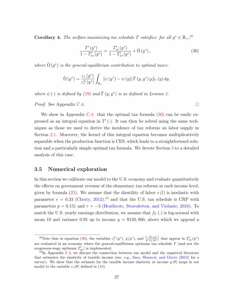
Corollary 4. The welfare-maximizing tax schedule T satisfies: for all y⇤ 2 R+,32

T 0(y⇤)

1� T 0ex

(y⇤)=

T 0ex

(y⇤)

1� T 0ex

(y⇤)+

˜

⌦ (y⇤) , (30)

where ˜

⌦ (y⇤) is the general-equilibrium contribution to optimal taxes:

˜

⌦ (y⇤) ="r (y

⇤)

"Sr (y⇤)

ˆR+

[ (y⇤)� (y)] ˜� (y, y⇤) yfY (y) dy,

where (·) is defined by (29) and ˜

� (y, y⇤) is as defined in Lemma 2.


We show in Appendix C.4. that the optimal tax formula (30) can be easily ex-pressed as an integral equation in T 0

(·). It can then be solved using the same tech-niques as those we used to derive the incidence of tax reforms on labor supply inSection 2.1. Moreover, the kernel of this integral equation becomes multiplicativelyseparable when the production function is CES, which leads to a straightforward solu-tion and a particularly simple optimal tax formula. We devote Section 5 to a detailedanalysis of this case.

3.5 Numerical exploration

In this section we calibrate our model to the U.S. economy and evaluate quantitativelythe effects on government revenue of the elementary tax reforms at each income level,given by formula (25). We assume that the disutility of labor v (l) is isoelastic withparameter e = 0.33 (Chetty, 2012),33 and that the U.S. tax schedule is CRP withparameters p = 0.151 and ⌧ = �3 (Heathcote, Storesletten, and Violante, 2016). Tomatch the U.S. yearly earnings distribution, we assume that fY (·) is log-normal withmean 10 and variance 0.95 up to income y = $150, 000, above which we append a

32Note that in equation (30), the variables "Sr (y⇤), g (y⇤), and 1�FY (y⇤)y⇤fY (y⇤) that appear in T 0

ex

(y⇤)

are evaluated in an economy where the general-equilibrium optimum tax schedule T (and not theexogenous-wage optimum T 0

ex

) is implemented.33In Appendix F.2, we discuss the connection between our model and the empirical literature

that estimates the elasticity of taxable income (see, e.g., Saez, Slemrod, and Giertz (2012) for asurvey). We show that the estimate for the taxable income elasticity at income y (✓) maps in ourmodel to the variable "r(✓) defined in (10).

27

Pareto distribution with coefficient ⇡ = 1.5, i.e., lim

y!1E [y|y � y] /y =

⇡⇡�1 = 3 (Dia-

mond and Saez, 2011). As in Saez (2001), we obtain the distribution of wages w(✓)

from the earnings distribution and the individual first-order conditions (1). Afterchoosing values for the elasticities of substitution, we can infer the remaining param-eters of the production function. See Appendix F.1 for a more detailed description ofthe calibration procedure. We first study the case of a CES production function andthen extend our results to a Translog production function, for which the elasticitiesof substitution are distance-dependent.

CES production function

We first assume that the production function is CES and illustrate numerically theanalytical result of Corollary 3. We choose an elasticity of substitution � 2 {0.6 ; 3.1}.The value � = 0.6 is taken from Dustmann, Frattini, and Preston (2013) who studythe impact of immigration along the U.K. wage distribution and, as in our framework,group workers according to their position in the wage distribution.34,35 The value� = 3.1 is taken from Heathcote, Storesletten, and Violante (2016), who structurallyestimate this CES parameter for the U.S. by targeting cross-sectional moments of thejoint equilibrium distribution of wages, hours, and consumption. There is no clearconsensus in the empirical literature on how responsive relative wages are to changesin labor supply, and therefore on the appropriate value of �;36 our two values are onthe lower and higher sides of the typical empirical estimates.

Our results for the CES specification are illustrated in Figure 1. We plot thegovernment revenue impact of elementary tax reforms at each income level in themodel with exogenous wages (i.e., equation (20), illustrated by the red bold curve)and in general equilibrium (i.e., equation (28), illustrated by the black dashed curve),

34This literature is a useful benchmark because it studies the impact on relative wages of laborsupply shocks of certain skills, which is exactly the channel we want to analyze in our tax setting(except that for us the labor supply shocks are caused by tax reforms rather than immigrationinflows).

35Card (1990) and Borjas et al. (1997) also mesaure the skill type by the relative wage positionwhen studying the impact of immigration on native wages. The setting of Dustmann, Frattini, andPreston (2013) fits our setting particularly well because they group workers into fine groups: 20groups that contain 5% of the workforce respectively. In Appendix F.3, we formally show that theelasticity of substitution estimated in a framework with discrete earnings groups (e.g., percentilesor quartiles) can be used to calibrate a CES production function with a continuum of types.

36See, e.g., the debate on the impact of immigration on natives’ wages (Peri and Yasenov, 2015;Borjas, 2015).

28

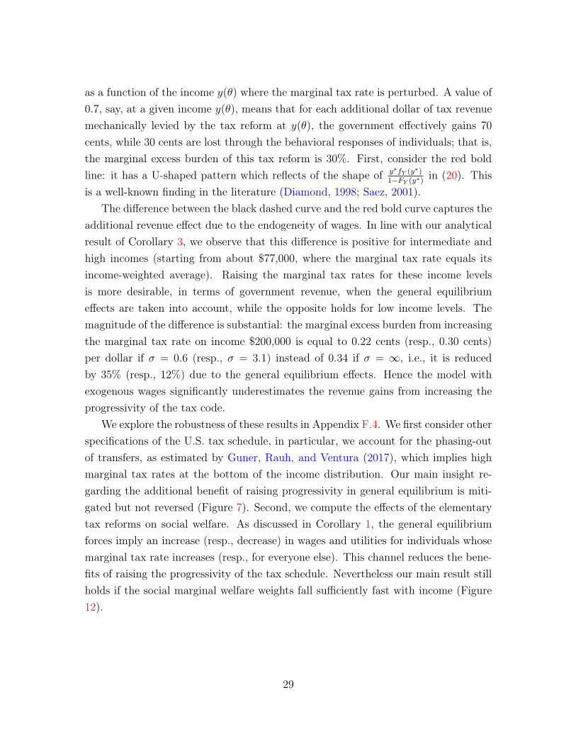
as a function of the income y(✓) where the marginal tax rate is perturbed. A value of0.7, say, at a given income y(✓), means that for each additional dollar of tax revenuemechanically levied by the tax reform at y(✓), the government effectively gains 70cents, while 30 cents are lost through the behavioral responses of individuals; that is,the marginal excess burden of this tax reform is 30%. First, consider the red boldline: it has a U-shaped pattern which reflects of the shape of y⇤fY (y⇤)

1�FY (y⇤) in (20). Thisis a well-known finding in the literature (Diamond, 1998; Saez, 2001).

The difference between the black dashed curve and the red bold curve captures theadditional revenue effect due to the endogeneity of wages. In line with our analyticalresult of Corollary 3, we observe that this difference is positive for intermediate andhigh incomes (starting from about $77,000, where the marginal tax rate equals itsincome-weighted average). Raising the marginal tax rates for these income levelsis more desirable, in terms of government revenue, when the general equilibriumeffects are taken into account, while the opposite holds for low income levels. Themagnitude of the difference is substantial: the marginal excess burden from increasingthe marginal tax rate on income $200,000 is equal to 0.22 cents (resp., 0.30 cents)per dollar if � = 0.6 (resp., � = 3.1) instead of 0.34 if � = 1, i.e., it is reducedby 35% (resp., 12%) due to the general equilibrium effects. Hence the model withexogenous wages significantly underestimates the revenue gains from increasing theprogressivity of the tax code.

We explore the robustness of these results in Appendix F.4. We first consider otherspecifications of the U.S. tax schedule, in particular, we account for the phasing-outof transfers, as estimated by Guner, Rauh, and Ventura (2017), which implies highmarginal tax rates at the bottom of the income distribution. Our main insight re-garding the additional benefit of raising progressivity in general equilibrium is miti-gated but not reversed (Figure 7). Second, we compute the effects of the elementarytax reforms on social welfare. As discussed in Corollary 1, the general equilibriumforces imply an increase (resp., decrease) in wages and utilities for individuals whosemarginal tax rate increases (resp., for everyone else). This channel reduces the bene-fits of raising the progressivity of the tax schedule. Nevertheless our main result stillholds if the social marginal welfare weights fall sufficiently fast with income (Figure12).

29

0 50 100 150 200 250 3000.6

0.65

0.7

0.75

0.8

0.85

0.9

0.95

1R

evenue E

ffect

0 50 100 150 200 250 3000.6

0.65

0.7

0.75

0.8

0.85

0.9

0.95

1

Revenue E

ffect

Figure 1: Revenue gains of elementary tax reforms at each income y(✓). Red bold lines: exogenouswages (equation (20)). Black dashed lines: CES technology with � = 0.6 (left panel) and � = 3.1

(right panel) (equation (28)).

Translog production function

A criticism of the CES production function with a continuum of types is that high-skillworkers (say) are equally substitutable with middle-skill workers as they are with low-skill workers. We therefore propose a more flexible parametrization of the productionfunction that allows us to obtain distance-dependent elasticities of substitution, i.e.,such that closer skill types are stronger substitutes.37

Specifically, in this paragraph we explore quantitatively the implications of thetranscendental-logarithmic (Translog) production function. This specification can beused as a second-order local approximation to any production function (Christensen,Jorgenson, and Lau, 1973). With a continuum of labor inputs, its functional form isgiven by

lnF�

{L (✓)}✓2⇥�

= a0 +

ˆ⇥

a (✓) lnL (✓) d✓ + . . .

1

2

ˆ⇥

� (✓) (lnL (✓))2 d✓ +1

2

ˆ⇥⇥⇥

� (✓, ✓0) (lnL (✓)) (lnL (✓0)) d✓d✓0,(31)

where for all ✓, ✓0,´⇥ a (✓0) d✓0 = 1, � (✓, ✓0) = � (✓0, ✓), and � (✓) = �

´⇥ � (✓, ✓

0) d✓0.

These restrictions ensure that the technology has constant returns to scale. When� (✓, ✓0) = 0 for all ✓, ✓0, the production function is Cobb-Douglas.

37Teulings (2005) obtains this distance-dependent property in an assignment model.

30

The elasticity of substitution between the labor of types ✓ and ✓0 is given by

� (✓, ✓0) =

1 +

✓

1

⇢(✓)+

1

⇢(✓0)

◆

�(✓, ✓0)

��1

,

where ⇢ (✓) =

w(✓)L(✓)F (L ) =

y(✓)f(✓)E(y) denotes the type-✓ labor share of output.38 To

obtain distance-dependent elasticities, we propose the following specification of theexogenous parameters:

� (✓, ✓0) =

✓

1

⇢c(✓)+

1

⇢c(✓0)

◆�1

c1 � c2 exp

✓

� 1

2s2(yc(✓)� yc(✓0))

2

◆�

,

where c1, c2 are constants, and where ⇢c(✓) and yc(✓) are the current (i.e., empiricallymeasured given the actual tax system) income share and income of type ✓. Thelocal (i.e., such that ⇢(✓) = ⇢c(✓) and y(✓) = yc(✓)) elasticity of substitution betweenworkers in percentiles ✓ and ✓0 is then given by

� (✓, ✓0) =

⇢

1 + c1

c2 � exp

✓

� 1

2s2(yc(✓)� yc(✓0))

2

◆��1

. (32)

The parameters c1 and c2 determine the values of the elasticity of substitution betweentypes (✓, ✓0) with |y(✓)� y(✓0)| ! 1 and ✓ ⇡ ✓0, respectively. The parameter s

specifies the rate at which � (✓, ✓0) falls as ✓0 moves away from ✓.The left panel of Figure 2 shows the elasticity of substitution �(✓, ✓0) as a function

of ✓ for such a specification, where � (✓, ✓0) varies between 0.5 and 10. We let ✓ 2 ⇥ =

[0, 1] be the agent’s percentile in the income distribution. We choose two values for ✓0:the type that earns the median income ($33,500) and the type at the 95th percentileof the income distribution ($126,500), i.e., ✓0 = 0.5 (red bold line) and ✓0 = 0.95 (blackdashed line). This illustrates how substitutable is the labor supply of a given skilltype, measured by its income level y(✓) on the x-axis, with the skills at the medianand the 95th percentile. By construction, the elasticity of substitution equals 10 as✓ ! ✓0, then decreases with the distance |✓ � ✓0|, and converges to a value of 0.5 as✓ ! 1. As a comparison, we also plot the elasticity of substitution for a Cobb-Douglasproduction function, which is equal to 1 for any pair of types (✓, ✓0). In Appendix F.4we illustrate the cross-wage elasticities � (✓, ✓0) and also explore alternative Translogspecifications.

38We derive all of our results about the Translog production function in Appendix A.2.2.

31

0 50 100 150 200 250 3000

2

4

6

8

10

0 50 100 150 200 250 3000.6

0.65

0.7

0.75

0.8

0.85

0.9

0.95

1

Revenue E

ffect

Figure 2: Left panel: Red bold (resp., black dashed) line: elasticity of substitution between typeswith income y (✓) and the 50th (resp., 95th) percentile, for the Translog specification (32). Bluedashed-dotted lines: Cobb-Douglas specification. Right panel: Black dashed line (resp., red boldline, blue dashed-dotted line): Revenue gains of elementary tax reforms at income y(✓) for theTranslog specification (32) (resp., for exogenous wages, Cobb-Douglas production).

The right panel of Figure 2 plots the incidence on government revenue of theelementary tax reforms at each income y(✓) (equation 25) for the Translog specifi-cation (32) (black dashed curve) and compares them to the Cobb-Douglas technol-ogy (blue dashed-dotted curve). The general-equilibrium contribution with distance-dependence is also positive for high incomes and of slightly larger magnitude.

4 Generalizations

In this section we show how the methodology and the results of Section 1 can be gen-eralized to alternative and more sophisticated environments. We only briefly describethese extensions here; all of the details and proofs are gathered in Appendix D.

4.1 Income effects

In this section we extend the model of Section 1 to a general utility function overconsumption and labor supply U (c, l), where Uc, Ucc > 0 and Ul, Ull < 0. Thisspecification allows for arbitrary substitution and income effects. The definitionsof the structural cross- and own-wage elasticities � (✓, ✓0) and ↵ (✓) are identical to(8) and (9). We define the compensated (Hicksian) elasticity of labor supply withrespect to the retention rate "Sr (✓) and the income effect "SR (✓) as in (6), exceptthat e (✓) in the numerator is replaced by the standard expressions for, respectively,

32

ecr (✓) =

@ ln l(✓)@ ln r(✓)

�

�

uand eR (✓) = r (✓)w (✓) @l(✓)

@R, given by (55) and (56) in Appendix

D.1.1.39 The labor supply elasticity with respect to the wage "Sw (✓) is now defined by"Sw (✓) = (1� p (y (✓))) "Sr (✓) + "SR (✓). The other elasticities are then defined exactlyas in Section 1; in particular, the GE cross-wage elasticity � (✓, ✓0) is defined by (13),using the generalized expression for "w (✓).

With these general preferences, the incidence of an arbitrary tax reform ⌧ onindividual labor supply is given by the following formula, which generalizes (12):

ˆl (✓) = ˆlpe

(✓) + "w (✓)

ˆ⇥

� (✓, ✓0) ˆlpe

(✓0) d✓0, (33)

where "w (✓), and � (✓, ✓0) are replaced by their generalized definitions, and where

ˆlpe

(✓) ⌘ �"r (✓)⌧ 0 (y (✓))

1� T 0(y (✓))

+ "R (✓)⌧ (y (✓))

(1� T 0(y (✓))) y (✓)

.

The interpretation of this formula is identical to that of (12), except that the partial-equilibrium impact of the reform ˆl

pe

(✓) is modified: in addition to the substitutioneffect already described in the quasilinear model, labor supply now also rises by anamount proportional to "R (✓) due to an income effect induced by the higher totaltax payment ⌧ (y (✓)) of agent ✓.40 The (closed-form) incidence on wages, utilitiesand government revenue are then derived identically to the corresponding formulasin Section 2. Adding income effects to the basic framework therefore does not addany difficulty to our tax incidence analysis.

We can also generalize the result of Corollary 3 characterizing the incidence of taxreforms on government revenue. Suppose in addition to the assumptions of Corrolary3 that the utility function has the form U (c, l) = c1�⌘

1�⌘� l1+

1"

1+ 1"

. The revenue effect ofthe elementary tax reform at income y⇤ is then given by

dR (y⇤) = dRex

(y⇤) (34)

+ � "SrT 0

(y⇤)� ¯T 0

1� T 0(y⇤)

y⇤fY (y⇤)

1� FY (y⇤)� � "Sr ⌘ E

T 0(y)� ¯T 0

1� T 0(y)

|y > y⇤�

,

where ¯T 0= E [yT 0

(y)] /Ey is the income-weighted average marginal tax rate in the

39See, e.g., p. 208 in Saez (2001).40The partial-equilibrium formula for ˆl

pe

(✓) is identical to that derived in models with exogenouswages by Saez (2001) and Golosov, Tsyvinski, and Werquin (2014) (Proposition 1), except that thatnow the elasticities "r (✓) and "R (✓) take into account the own-wage effects ↵ (✓).

33

economy and where � is as defined in Corollary 3. Note that for ⌘ = 0, this formulareduces to equation (28). If ⌘ > 0 and the baseline tax schedule is progressive, thenthe second general-equilibrium contribution has the opposite sign of the first. If topincomes are Pareto distributed and the baseline tax schedule is CRP, we derive inAppendix D.1.2 a necessary and sufficient condition on the progressivity parameterp, the Pareto coefficient and the curvature of the utility function ⌘ such that thefirst general-equilibrium term in (34) is larger than the second as y ! 1. Forempirically plausible values of the income effect parameter, the magnitude of thegeneral-equilibrium contribution to government revenue incidence obtained in Section3.5 is reduced by a third (and hence keeps the same direction).

4.2 Several sectors or education levels

The aggregate production function F assumed in Section 1 takes as inputs the laborsupply of each one-dimensional skill type ✓ 2 ⇥. In this framework, the skill ✓ ofan agent can be interpreted as her percentile in the wage distribution {w (✓)}✓2⇥.Suppose now that the population is divided into N groups (e.g., sectors, educationlevels, etc.). Each group i is composed of a continuum of agents indexed by their skill✓ 2 ⇥ who earn wage wi (✓). The assignment of each individual to a given group i isexogenous. Note that the wage distributions {wi (✓)}✓2⇥ and {wj (✓)}✓2⇥ of differentgroups i 6= j overlap.

The aggregate production function is now defined by

F⇣

{Li (✓)}(✓,i)2⇥⇥{1,...,N}

⌘

, (35)

where Li (✓) is the aggregate labor supply of the agents of type ✓ who work in sectori. Extending our analysis to this general production function is straightforward; thetechnical details are gathered in Appendix D.2.1. We define the wage, labor supply,and income of type ✓ in sector i by wi (✓), li (✓), and yi (✓) respectively. We define asin Section 1.2, for each pair of skills (✓, ✓0) and groups (i, j), the cross-wage elasticity�i,j (✓, ✓

0), the own-wage elasticity ↵i (✓), and the partial-equilibrium labor elasticities

"r,i (✓) , "w,i (✓). A change of variables then allows us to define, for each income-grouppair (y, i), the wage wy,i of the agents who earn income y in group i, and the N ⇥ 1

vector wy = (wy,i)i=1,...,N . We define analogously the vectors ly, ˆly, "r (y), "w (y),and the N ⇥N matrices � (y, y0) and � (y, y0). We show that the result of Lemma 1

34

is now replaced by a system of linear integral equations, which can be solved usinganalogous steps as those leading to Proposition 1. We obtain that the incidence ofan arbitrary tax reform ⌧ on individual labor supplies is given in closed-form by

ˆly =� "r (y)⌧ 0 (y)

1� T 0(y)

�ˆR+

Diag ("w (y))� (y, y0) "r (y0)

⌧ 0 (y0)

1� T 0(y0)

dy0. (36)

The interpretation of this formula is identical to that of (12), with the only differencethat the incidence of tax reforms now naturally depends on a larger number of (cross-sector) elasticities.

Example: High School and College labor

A special case of the general production function (35) is the so-called canonical model(Acemoglu and Autor, 2011), where individuals are categorized according to their levelof education (high school vs. college); this model has been studied empirically byKatz and Murphy (1992) and Card and Lemieux (2001). Let LH =

´✓lH(✓)✓gH(✓)d✓

and LC =

´⇥ lC(✓)✓gC(✓)d✓ denote the aggregate labor inputs in efficiency units

in sectors i = H,C, respectively, where sector H is composed of the high school-educated workers (with density gH over types ✓ 2 ⇥), and sector C is composed ofthe college-educated workers (with density gC over types ✓ 2 ⇥). Suppose finally thatthe aggregate production function is given by a CES aggregator of LH and LC , i.e.,

F =

h

L��1�

H + L��1�

C

i

��1

.

In this model, there is an infinite elasticity of substitution between workers withineach education level, and a finite and constant elasticity of substitution � across thetwo groups. The wage of an individual with type ✓ in the education group i 2 {H,C}is given by wi (✓) = @F/@Li (✓). In particular, we have wi(✓0)

wi(✓)=

✓0

✓for any two types

(✓, ✓0), so that the relative wages within each group i are given by the ratio of thecorresponding exogenous skills.

As we show in Appendix D.2.2, Corollary 3 can be easily extended to this envi-ronment. Suppose that the disutility of labor is isoelastic and that the initial taxschedule is CRP, so that the labor supply elasticities "Sr and "Sw are constant. We

35

obtain in this case

dR (y⇤) = dRex

(y⇤) + �"Sr [sC (y⇤)� sC ]¯T 0C � ¯T 0

H

1� T 0(y⇤)

y⇤fY (y⇤)

1� FY (y⇤), (37)

where dRex

(y⇤) is given by (20), ¯T 0i =´T 0

(y) yfY,i (y) dy is the income-weighted av-erage marginal tax rate in education group i = H,C, sC(y⇤) is the share of individualsearning y⇤ that are college-educated, sC is the share of aggregate income accruing tocollege-educated workers, and � is defined as in Corollary 3.

Comparing equation (37) to equation (28) reveals two differences arising fromthe alternative modeling of the production. The first is that the general-equilibriumeffect now depends on the difference between the average marginal tax rates in thetwo education groups (or sectors), rather than on the difference between the marginaltax rate at income y⇤ vs. in the population as a whole. This difference becomes clearif we interpret our production function in Section 1 as one that treats each skill ✓ asa distinct sector. Second, the general-equilibrium contribution features an additionalterm that captures the difference between the share of education group C at incomelevel y⇤ and the overall share of income accruing to group C. This term is positive ifcollege educated labor is over-represented at income level y⇤. This is because in thiscase an increase in the marginal tax rate at y⇤ raises wages in sector 1 and lowersthem in sector 2. Note that this new term is bounded above by 1, and is equal to 1 ifsector 1 is composed of all of the agents with type ✓⇤ (and only them), as is the casein Section 1.

4.3 Intensive and extensive margins

In this section we extend the model of Section 1 to an environment where individ-uals choose their labor supply both on the intensive margin (hours l conditional onparticipating in the labor force) and on the extensive margin (participation deci-sion). Heterogeneity is two-dimensional: individuals are indexed by their skill type✓ 2 [✓, ¯✓] and by their cost of working 2 R+. The utility function is given byU (c, l) = c � v (l) � I{l>0}, where I{l>0} is an indicator function equal to 1 if theagent is employed (i.e., l > 0). The intensive margin choice of labor effort l (✓) de-pends on the marginal tax rate T 0

(y (✓)), while the extensive margin choice consistsof a participation threshold ⇤ (✓) that depends on the average tax rate relative totransfers, T (y (✓))�T (0). The version of this model with exogenous wages has been

36

analyzed by Saez (2002).The elasticities ⌘ST (✓) and ⌘Sw (✓) of the participation rate at skill ✓ with respect

to the average tax rate and the wage are defined by the standard equations (71, 72)given in Appendix D.3. We then naturally define the partial-equilibrium elasticities⌘T (✓) and ⌘w (✓) by (73). These elasticities are determined by the reservation densityof agents with skill ✓ who are close to indifference between participation and non-participation in the initial tax system. The GE cross-wage elasticity � (✓, ✓0) is stilldefined by (13), except that "w (✓00) is now replaced by ("w (✓00) + ⌘w (✓00)) in each termof the resolvent series. The incidence of an arbitrary tax reform ⌧ on the total laborsupply L (✓) of agents of skill ✓ is given by the following formula, which generalizesProposition 1:

ˆL (✓) =ˆLpe

(✓) + ("w (✓) + ⌘w (✓))

ˆ⇥

� (✓, ✓0) ˆLpe

(✓0) d✓0, (38)

where "w (✓), and � (✓, ✓0) are replaced by their generalized definitions, and where

ˆLpe

(✓) ⌘ �"r (✓)⌧ 0 (y (✓))

1� T 0(y (✓))

� ⌘T (✓)⌧ (y (✓))

y (✓)� T (y (✓)) + T (0)

.

The interpretation of this formula is identical to that of (12), with two differences.First, the partial-equilibrium impact (ˆLpe

(✓)) is modified: in addition to the substi-tution effect already described in the quasilinear model, the tax reform now raises thetax payment of agents with skill ✓ by ⌧ (y (✓)), which lowers the total labor supply ofthat skill by an amount proportional to ⌘T (✓), by inducing those with a large fixedcost of working to drop out of the labor force. Second, the change in the wage oftype ✓ induces a decrease in total hours (from both intensive and extensive marginresponses) given by ("w (✓) + ⌘w (✓)) rather than simply "w (✓). From this formula, itis straightforward to obtain the incidence of any tax reform on individual labor sup-plies, wages, participation thresholds, participation rates, utilities, and governmentrevenue. These are all derived in Appendix D.3. Adding participation decisions tothe basic framework therefore does not add any difficulty to the incidence analysis.

4.4 Other extensions

In Appendix D.4, we derive the incidence of tax reforms for other extensions of ourbaseline model, namely, the cases where the production function has non-constant

37

returns to scale and capital is an input in production. These extensions can be easilyanalyzed using the techniques we introduced in Section 2.

5 A simple analysis of optimal taxes

Our tax incidence analysis of Section 2 delivered a general formula for the optimaltax schedule in general equilibrium (Corollary 4). In this section, we simplify andanalyze it further by assuming that the production function is CES. This simplifyingassumption allows us to generalize parsimoniously and transparently the optimaltaxation formula of Diamond (1998), as all of the own- and cross-wage effects arethen summarized by a single elasticity of substitution �. This also allows us togeneralize the standard public finance results (closed-form expression for the optimaltop tax rate, U-shape of the marginal tax rates), and to immediately quantify themagnitude of the “Stiglitz effects” that arise in general equilibrium Stiglitz (1982)as a function of the degree of complementarity between skills in production. Wefinally provide robustness tests by computing the optimal tax schedule obtained forthe distance-dependent Translog specification introduced in Section 3.5.

5.1 Optimal tax schedule with CES technology

Recall that formula (30) is an integral equation that can be solved to obtain theoptimal tax rates.41 In the case of a CES production function, this integral equationhas a multiplicatively separable kernel and can thus be easily solved. We obtain thefollowing proposition:

41Note that the income distribution is endogenous in the formula for optimal tax rates (39). Asdiscussed in Section 1.1, there exists a monotone mapping between incomes and skills whenever themapping between wages and skills is monotone – and this is w.l.o.g. because we can always relabelthe type ✓ as the agent’s position in the wage distribution. One caveat applies, however: as taxeschange, the ordering of types may also change. Thus, expression (30) assumes that skills are orderedgiven the optimum tax schedule, rather than given the existing (suboptimal) tax code that may beused for the calibration in numerical simulations. Nevertheless, we show in Appendix A.2.3. thatwhen the production function is CES (which we assume throughout Section 5), the ordering of typesnever changes, independently of the (possibly non-local) tax reform that is implemented, as long asthe resulting tax function is differentiable. Moreover, in all of our numerical explorations for optimalincome taxes using a Translog production function, the ordering of types is always the same for theoptimal tax schedule and for the tax schedule to which the economy is calibrated.

38

Proposition 3. Assume that the production function is CES with elasticity of sub-stitution � > 0. Then the optimal marginal tax rate at income y⇤ satisfies

T 0(y⇤)

1� T 0(y⇤)

=

1

"r (y⇤)(1� g (y⇤))

1� FY (y⇤)

y⇤fY (y⇤)+

g (y⇤)� 1

�. (39)

Proof. See Appendix E.1.

The first term on the right hand side of (39) is analogous to the optimal taxformula obtained in the model with exogenous wages (Diamond, 1998; Saez, 2001):the marginal tax rate at income y⇤ is proportional to the inverse elasticity of labor"r(y

⇤) and to the hazard rate of the income distribution 1�FY (y⇤)

y⇤fY (y⇤) , and is decreas-ing in the average marginal social welfare weight g(y⇤). The only difference is thatthe relevant labor supply elasticity "r (y

⇤) accounts for the own-wage effects. Since

"r (y⇤) =

"Sr (y⇤)

1+"Sw(y⇤)/� < "Sr (y⇤), this tends to raise optimal marginal tax rates, more so

for lower values of the elasticity of substitution �. Intuitively, increasing the marginaltax rate at y⇤ leads these agents to lower their labor supply, which raises their ownwage and thus reduces the behavioral response.

The second term, (g(y⇤)� 1) /�, which works in the opposite direction, capturesthe fact that the wage and welfare of type ✓⇤ increase due to a higher marginal tax rateT 0(y⇤), at the expense of the other individuals whose wage and welfare decrease (see

Corollary 1). Suppose that the government values the welfare of individuals ✓⇤ lessthan average, i.e., g (y⇤) < 1.42 This negative externality induced by the behavior of✓⇤ implies that the cost of raising the marginal tax rate at y⇤ is higher than in partialequilibrium, and tends to lower the optimal tax rate. Conversely, the governmentgains by raising the optimal tax rates of individuals y⇤ whose welfare is valued morethan average, i.e., g (y⇤) > 1. This induces these agents to work less and earn a higherwage, which makes them strictly better off, at the expense of the other individuals inthe economy, whose wage decreases. This term is therefore a force for higher marginaltax rates at the bottom and lower marginal tax rates at the top if the governmenthas a strictly concave (redistributive) social objective.

Formula (39) parsimoniously generalizes the optimal tax formula derived by Dia-mond (1998) and Saez (2001) assuming exogenous wages (� = 1) to a general CESproduction function. It depends on one additional sufficient statistic, namely, the

42Since lump-sum transfers are available to the government, the average marginal social welfareweight in the economy is equal to 1.

39

elasticity of substitution between skills in production �. This formula also extendsthe general-equilibrium analysis of Stiglitz (1982) in a model with two skills to theworkhorse framework of taxation, i.e., with a continuum of types and arbitrary non-linear taxes. It allows us to go beyond the purely qualitative insights obtained in thetwo-type framework and make operational the theory of optimal tax design in generalequilibrium. In particular, we show in the next two subsections how the key resultsobtained with exogenous wages, namely, the characterization of the optimal top taxrate and the U-shape of marginal tax rates, are affected.

5.2 Top tax rate

We now derive the implications of formula (39) for the optimal top tax rate. Let⇡ > 1 denote the Pareto coefficient of the tail of the income distribution in the data,that is, 1� FY (y) ⇠

y!1c/y⇡ for some constant c.

Corollary 5. Assume that the production function is CES with elasticity of substi-tution � > 0 and that the disutility of labor is isoelastic with parameter e. Assumemoreover that given the current tax schedule, incomes are Pareto distributed at thetail with coefficient ⇡ > 1, and that the top marginal tax rate that applies to theseincomes is constant. Assume finally that the marginal social welfare weights at the topconverge to g (given the optimal tax schedule). Then the top tax rate of the optimaltax schedule satisfies

⌧ ⇤ =1� g

1� g + ⇡ "r ⇠, (40)

with "r = e1+e/�

and ⇠ = (1� ⇡"r/�)�1. In particular, ⌧ ⇤ is strictly smaller than the

optimal top tax rate in the model with exogenous wages (� = 1).

Proof. See Appendix E.2. The non-trivial part of the proof consists of showing thatfor a CES production function, if the income distribution has a Pareto tail in the data,then it has the same Pareto tail at the optimum, even though the wage distributionis endogenous.

Formula (40) generalizes the familiar top tax rate result of Saez (2001) (in which"r = "Sr and ⇠ = 1) to a CES production function. There is one new sufficient statistic,the elasticity of substitution between skills in production �, that is no longer restrictedto being infinite. This proposition implies a strictly lower top marginal tax rate thanif wages were exogenous. Immediate calculations of the optimal top tax rate illustrate

40

the power of this formula. Suppose that g = 0, ⇡ = 2, e = 0.5, and � = 1.5.43 Weimmediately obtain that the optimal tax rate on top incomes is equal to ⌧ ⇤ex = 50% inthe model with exogenous wages, and falls to ⌧ ⇤ = 40% once the general equilibriumeffects are taken into account. Suppose instead that ⇡ = 1.5 and e = 0.33, then weget ⌧ ⇤ex = 66% and ⌧ ⇤ = 64%. In this case the trickle-down forces barely affect theoptimum tax rate quantitatively. Figure 3 shows more comprehensive comparativestatics.44

0.2 0.3 0.4 0.5 0.60.3

0.4

0.5

0.6

0.7

0.8

Top T

ax

Rate

0.5 1 1.5 2 2.5 3 3.50.3

0.4

0.5

0.6

0.7

0.8

Top T

ax

Rate

Figure 3: Optimal top tax rate as a function of the labor supply elasticity e (left panel, � = 3.1

fixed) and the elasticity of substitution � (right panel, e = 0.33 fixed) and for varying Paretoparameters ⇡.

5.3 U-shape of optimal marginal tax rates

We finally analyze the impact of general equilibrium on the shape of optimal taxrates. Suppose for simplicity that the social planner is Rawlsian, i.e., it maximizesthe lump-sum component of the tax schedule, so that g (y) = 0 for all y > 0.45

The partial-equilibrium equivalent of formula (39) for optimal taxes (for which thesecond term on the right hand side is equal to zero) generally implies a U-shapedpattern of marginal tax rates (Diamond, 1998; Saez, 2001) because the hazard rate1�FY (y)yfY (y) is a U-shaped function of income y. If this is the case, then the additional

term �1/� < 0 in (39) leads to a general equilibrium correction for T 0(·) that is also

43These values are meant to be only illustrative but they are in the range of those estimated inthe empirical literature. See the calibration in Section 3.5.

44See also Green and Phillips (2015) who study quantitatively the size of the optimal top tax ratein a two-sector model.

45Thus, if the income of the lowest type is positive, we assume that there are some additionalagents in the economy who are unable to work and whose consumption equals the demogrant.

41

U-shaped, because the optimal marginal tax rate T 0(y⇤) is increasing and concave in

the right hand side of (39).46 This suggests that the general equilibrium forces tendto reinforce the U-shape of the optimum tax schedule.

To formalize this intuition using our tax incidence analysis of Section 2, we startby defining a benchmark optimal tax schedule with exogenous wages, to which wecan compare our general-equilibrium formula.

Defining a benchmark with exogenous wages. First, we define the marginaltax rates that a partial-equilibrium planner would set from Diamond (1998) usingthe same data to calibrate the model, and making the same assumptions about theutility function, but wrongly assuming that the wage distribution is exogenous:

T 0ex

(y (✓))

1� T 0ex

(y (✓))=

✓

1 +

1

"Sr (w(✓))

◆

1� FW (w(✓))

fW (w(✓))w(✓), (41)

where w(✓) are the wages inferred from the data, i.e., obtained from the incomesobserved empirically and the first-order conditions (1), and FW is the correspondingwage distribution. Formula (41) is the benchmark to which we compare our optimalpolicy results numerically, thus directly highlighting how our policy implications differfrom those of Diamond (1998).

A government that would implement this tax formula, however, would then ob-serve that the implied distribution of wages does change and is not consistent withthe optimality of the tax schedule (41). To overcome this inconsistency, we considera self-confirming policy equilibrium (SCPE) T 0

scpe

(y (✓)), as originally proposed byRothschild and Scheuer (2013, 2016), which is such that implementing the tax sched-ule (41) generates a wage distribution given which these tax rates are optimal – inother words, this construction solves for the fixed point between the wage distributionand the tax schedule. We use this concept as our exogenous-wage benchmark for ourtheoretical analysis below.

Comparing optimal taxes to those obtained with exogenous wages. Wecan apply our tax incidence result of Proposition 2 using the SCPE tax schedule asour initial tax schedule. This exercise gives the (first-order) welfare gains of reforming

46That is, if the function h(y)1+h(y) with h (y) = 1

"r(y)1�FY (y)yfY (y) is U-shaped, it is easy to check that the

general-equilibrium correction to marginal tax rates y 7! h(y)��1

1+h(y)��1 � h(y)1+h(y) is then also U-shaped.

42

this tax schedule at any income level, and hence the shape of the general-equilibriumcorrection to the optimal policy obtained assuming exogenous wages. We provide thecorresponding incidence formula for a general CES technology in Appendix E.3, andfocus on the simpler Cobb-Douglas case (� = 1) here.

Corollary 6. Suppose that the production function is Cobb-Douglas (� = 1), thatthe initial tax schedule T = T

scpe

is the SCPE, and that the disutility of labor isisoelastic with parameter e. The incidence of the elementary tax reform at income y⇤

on government revenue (or Rawlsian welfare) is given by

dRscpe

(y⇤) = 1� ⇣1

T 0(y⇤)

⇥

p(y⇤) +1

e

⇤

, (42)

where ⇣�1 ⌘ 1T 0 [p+

1e] > 0 is a constant that depends on the income-weighted averages

of the marginal tax rate ¯T 0= E[ y

EyT0(y)] and of the local rate of progressivity p =

E[ yEyp (y)] in the initial economy.

Proof. See Appendix E.3.

The map y⇤ 7! dRscpe

(y⇤) in (42) gives the shape of the general-equilibrium cor-rection to the optimal tax schedule obtained assuming exogenous wages. Importantly,just as the result of Corollary 3, formula (42) shows that the general-equilibrium ef-fects of the tax reform have a shape that is inherited from that of the initial taxschedule. In particular, if the marginal tax rates T 0

(y⇤) of the SCPE are U-shapedas a function of income, the term �1/T 0

(y⇤) in equation (42) leads to a general-equilibrium correction that is itself U-shaped. Note, however, that the additionalterm in general equilibrium depends also on the rate of progressivity p (y⇤) of the ini-tial (SCPE) tax schedule. Nevertheless, since

�

�p (y⇤)�

� < 1 ⌧ 1e⇡ 3 (Chetty (2012)),

the shape of dR (y⇤) as a function of y⇤ is mostly driven by the term �1/T 0(y⇤); our

numerical simulations below confirm this intuition.

5.4 Numerical simulations

Our calibration is similar to that in Section 3.5, see Appendix F.1 for details. Through-out this section we consider a Rawlsian social objective. In Appendix F.5.2 we simu-late optimal taxes for concave social welfare functions G; our results are similar.

43

The role of the elasticity of substitution. The left panel of Figure 4 plots theoptimal marginal tax rates as a function of types47 for two different values of theelasticity of substitution, and for the exogenous-wage planner defined in (41). Thelatter schedule has a familiar U-shape (Diamond, 1998; Saez, 2001). In line withour theoretical results of Section 5.1, the top tax rate is lower in general equilibriumand decreasing with �. Moreover, the optimal marginal tax rates are reduced by aneven larger amount at income levels close to the bottom of the U (around $100,000),and are higher at low income levels (below $40,000).48 This confirms our findings ofCorollary 6 and implies that the U-shape obtained for exogenous-wages is reinforcedby the general equilibrium considerations.

Translog production function. In the right panel of Figure 4, we illustrate theoptimal marginal tax rates in case of the Translog production function with distance-dependent elasticities of substitution, as calibrated in Section 3.5, and compare it tothe optimal tax schedule in the case of a Cobb-Douglas production function; the graphshows that the policy implications are hardly altered, which justifies our focus on thecase of a CES production for the theoretical analysis of this section. In AppendixF.5.3, we consider alternative Translog specifications and obtain similar conclusions.

47The scale on the horizontal axis on the left panel is measured in income; e.g., the value ofthe optimal marginal tax rate at the notch $100,000 is that of a type ✓ who earns an incomey (✓) = $100, 000 in the calibration to the U.S data. The income that this type earns in the optimalallocation is generally different (see the right panel). In Appendix F.5.1, we also provide the optimaltax schedule as a function of incomes at the optimum.

48Since the exogenous-wage tax rates are already very high at those low income levels, the generalequilibrium effects are quantitatively very small (at most 1.8 percentage points).

44

0 100 200 300 400 500

Type Expressed by Current Income in $1,000

0.2

0.3

0.4

0.5

0.6

0.7

0.8

0.9

1M

arg

inal T

ax

Rate

sExogenous-Wage PlannerElasticity of Substitution 3.1Elasticity of Substitution .6

0 100 200 300 400 5000.2

0.3

0.4

0.5

0.6

0.7

0.8

0.9

1

Figure 4: Optimal marginal tax rates as a function of types. Black dashed lines: exogenous wages.Left panel: CES technology with � = 3.1 (red bold line) and � = 0.6 (blue dashed-dotted line).Right panel: Translog technology (32) (blue dashed-dotted line) and Cobb-Douglas (� = 1) (redbold line).

U-shape of the general-equilibrium effect. Next, we plot in Figure 5 the shapeof the general-equilibrium correction to the optimal taxes obtained in the model withexogenous wages. We do so by applying our incidence formula (25) using (41) (i.e.,the black-dotted curve in Figure 4) as our initial tax schedule. Recall that Corollary6 addresses the same question analytically using the SCPE as the exogenous-wagebenchmark. The red bold line plots the effects of the tax reform according to theexogenous-wage planner (41). These effects are uniformly equal to zero by construc-tion. The black dashed line shows that when the low-income marginal tax ratesare high (as in the exogenous-wage optimum) rather than low (as in the CRP taxcode assumed in Corollary 3), the general equilibrium forces call for lower tax ratesfor intermediate and high incomes, and higher marginal tax rates for low incomes.This graph implies that starting from the exogenous-wage optimum, the gains fromperturbing the marginal tax rates are themselves U-shaped and negative, except atthe very bottom of the income distribution, thus confirming our theoretical result ofCorollary 6.

Conclusion

In this paper we have developed a variational approach for the study of nonlinear taxreforms in general equilibrium. It can be used to study the incidence of reforming agiven baseline tax schedule, e.g. the current U.S. tax code, as well as to characterize

45

0 50 100 150 200 250 300-0.15

-0.1

-0.05

0

0.05

0.1

0.15

0.2

0.25

Norm

alized R

evenue E

ffect

Figure 5: Tax incidence around the exogenous-wage optimum (41). Red bold line: model withexogenous wages. Black dashed line: CES production function (� = 3.1).

the optimal tax schedule. The key methodological tool that we brought into the anal-ysis is the concept of integral equations. Our variational approach is powerful in thatit allows to analyze sophisticated environments (with general individual preferencesand choice variables, general production structures, etc.) with no additional technicaldifficulties as in the simpler baseline model.

References

Acemoglu, D. and D. Autor (2011): “Skills, Tasks and Technologies: Implica-tions for Employment and Earnings,” in Handbook of Labor Economics Vol. 4, ed.by O. Ashenfelter and D. Card, Elsevier, 1043–1171.

Ales, L., A. A. Bellofatto, and J. J. Wang (2017): “Taxing Atlas: Executivecompensation, firm size, and their impact on optimal top income tax rates,” Reviewof Economic Dynamics, 26, 62–90.

Ales, L., M. Kurnaz, and C. Sleet (2015): “Technical change, wage inequality,and taxes,” The American Economic Review, 105, 3061–3101.

Ales, L. and C. Sleet (2016): “Taxing Top CEO Incomes,” American EconomicReview (forthcoming).

Antras, P., A. de Gortari, and O. Itskhoki (2016): “Globalization, Inequalityand Welfare,” Working Paper.

46

Bénabou, R. (2002): “Tax and Education Policy in a Heterogenous-Agent Economy:What of Levels of Redistribution Maximize Growth and Efficiency?” Econometrica,70, 481–517.

Borjas, G. J. (2003): “The Labor Demand Curve Is Downward Sloping: Reexam-ining the Impact of Immigration on the Labor Market,” The Quarterly Journal ofEconomics, 118, 1335–1374.

——— (2015): “The wage impact of the Marielitos: A reappraisal,” ILR Review.

Borjas, G. J., R. B. Freeman, L. F. Katz, J. DiNardo, and J. M. Abowd(1997): “How much do immigration and trade affect labor market outcomes?”Brookings papers on economic activity, 1997, 1–90.

Bucci, A. and P. Ushchev (2014): “The Sources of Sharing Externalities: Spe-cialization versus Competition,” Working Paper.

Card, D. (1990): “The impact of the Mariel boatlift on the Miami labor market,”ILR Review, 43, 245–257.

——— (2009): “Immigration and Inequality,” American Economic Review, 99, 1–21.

Card, D. and T. Lemieux (2001): “Can Falling Supply Explain the Rising Returnto College for Younger Men? A Cohort-Based Analysis,” Quarterly Journal ofEconomics, 116, 705–746.

Cesarini, D., E. Lindqvist, M. J. Notowidigdo, and R. Ostling (2017):“The Effect of Wealth on Individual and Household Labor Supply: Evidence fromSwedish Lotteries,” American Economic Review (forthcoming).

Chen, L. and C. Rothschild (2015): “Screening with endogenous preferences,”Working Paper.

Chetty, R. (2009): “Sufficient Statistics for Welfare Analysis: A Bridge BetweenStructural and Reduced-Form Methods,” Annu. Rev. Econ., 1, 451–488.

——— (2012): “Bounds on elasticities with optimization frictions: A synthesis ofmicro and macro evidence on labor supply,” Econometrica, 80, 969–1018.

Christensen, L. R., D. W. Jorgenson, and L. J. Lau (1973): “Transcendentallogarithmic production frontiers,” The Review of Economics and Statistics, 28–45.

47

Diamond, P. A. (1998): “Optimal Income Taxation: An Example with a U-ShapedPattern of Optimal Marginal Tax Rates,” American Economic Review, 88, 83–95.

Diamond, P. A. and J. A. Mirrlees (1971): “Optimal taxation and public pro-duction II: Tax rules,” The American Economic Review, 61, 261–278.

Diamond, P. A. and E. Saez (2011): “The Case for a Progressive Tax: FromBasic Research to Policy Recommendations,” Journal of Economic Perspectives,25, 165–90.

Dustmann, C., T. Frattini, and I. P. Preston (2013): “The effect of immi-gration along the distribution of wages,” The Review of Economic Studies, 80,145–173.

Fradera, I. (1986): “Perfect competition with product differentiation,” Interna-tional Economic Review, 529–538.

Fullerton, D. and G. E. Metcalf (2002): “Tax incidence,” Handbook of publiceconomics, 4, 1787–1872.

Golosov, M., A. Tsyvinski, and N. Werquin (2014): “A Variational Approachto the Analysis of Tax Systems,” Working Paper.

Green, R. K. and M. D. Phillips (2015): “Demand for’The 1%’: Tax Incidenceand Implications for Optimal Income Tax Rates,” Working Paper.

Guner, N., R. Kaygusuz, and G. Ventura (2014): “Income taxation of UShouseholds: Facts and parametric estimates,” Review of Economic Dynamics, 17,559–581.

Guner, N., C. Rauh, and G. Ventura (2017): “Means-Tested Transfers in theUS: Facts and Parametric Estimates,” Working Paper.

Harberger, A. C. (1962): “The incidence of the corporation income tax,” TheJournal of Political Economy, 215–240.

Hart, O. D. (1979): “Monopolistic competition in a large economy with differenti-ated commodities,” The Review of Economic Studies, 46, 1–30.

48

Heathcote, J., K. Storesletten, and G. L. Violante (2016): “Optimal taxprogressivity: An analytical framework,” Quarterly Journal of Economics (forth-coming).

Hendren, N. (2015): “The Policy Elasticity,” in Tax Policy and the Economy, Vol-ume 30, University of Chicago Press.

Hines, J. R. (2009): “Peter Mieszkowski and the General Equilibrium Revolution inPublic Finance,” in Proceedings. Annual Conference on Taxation and Minutes ofthe Annual Meeting of the National Tax Association, JSTOR, vol. 102, 213–216.

Imbens, G. W., D. B. Rubin, and B. I. Sacerdote (2001): “Estimating theeffect of unearned income on labor earnings, savings, and consumption: Evidencefrom a survey of lottery players,” American Economic Review, 778–794.

Itskhoki, O. (2008): “Optimal redistribution in an open economy,” Working Paper.

Jacquet, L. and E. Lehmann (2017): “Optimal Income Taxation with Composi-tion Effects,” IZA Discussion Paper No. 11019.

Katz, L. F. and K. M. Murphy (1992): “Changes in Relative Wages, 1963-1987:Supply and Demand Factors,” The Quarterly Journal of Economics, 107, 35–78.

Kleven, H., C. Kreiner, and E. Saez (2009): “The Optimal Income Taxation ofCouples,” Econometrica, 77, 537–560.

Kotlikoff, L. J. and L. H. Summers (1987): “Tax incidence,” Handbook of publiceconomics, 2, 1043–1092.

Kress, R. (2014): Linear integral equations (Third Edition), Springer.

Krusell, P., L. E. Ohanian, J.-V. Ríos-Rull, and G. L. Violante (2000):“Capital-skill complementarity and inequality: A macroeconomic analysis,” Econo-metrica, 68, 1029–1053.

Mirrlees, J. A. (1971): “An Exploration in the Theory of Optimum Income Taxa-tion,” The Review of Economic Studies, 38, 175–208.

Musgrave, R. A. and T. Thin (1948): “Income tax progression, 1929-48,” Journalof political Economy, 56, 498–514.

49

Peri, G. and V. Yasenov (2015): “The labor market effects of a refugee wave:Applying the synthetic control method to the Mariel boatlift,” Tech. rep., NationalBureau of Economic Research.

Piketty, T. (1997): “La redistribution fiscale face au chomage,” Revue françaised’économie, 12, 157–201.

Piketty, T. and E. Saez (2013): “A Theory of Optimal Inheritance Taxation,”Econometrica, 81, 1851–1886.

Piketty, T., E. Saez, and S. Stantcheva (2014): “Optimal taxation of toplabor incomes: A tale of three elasticities,” American Economic Journal: EconomicPolicy, 6, 230–271.

Polyanin, A. D. and A. V. Manzhirov (2008): Handbook of integral equations,CRC press.

Press, W. H. (2007): Numerical recipes 3rd edition: The art of scientific computing,Cambridge university press.

Rothschild, C. and F. Scheuer (2013): “Redistributive Taxation in the RoyModel,” The Quarterly Journal of Economics, 128, 623–668.

——— (2014): “A theory of income taxation under multidimensional skill heterogene-ity,” NBER Working Paper No. 19822.

——— (2016): “Optimal Taxation with Rent-Seeking,” Review of Economic Studies(forthcoming).

Rothstein, J. (2010): “Is the EITC as good as an NIT? Conditional cash transfersand tax incidence,” American Economic Journal: Economic Policy, 2, 177–208.

Saez, E. (2001): “Using Elasticities to Derive Optimal Income Tax Rates,” Reviewof Economic Studies, 68, 205–229.

——— (2002): “Optimal Income Transfer Programs: Intensive versus Extensive La-bor Supply Responses,” Quarterly Journal of Economics, 117, 1039–1073.

Saez, E., J. Slemrod, and S. H. Giertz (2012): “The elasticity of taxable in-come with respect to marginal tax rates: A critical review,” Journal of economicliterature, 50, 3–50.

50

Saez, E. and S. Stantcheva (2016): “Generalized Social Marginal Welfare Weightsfor Optimal Tax Theory,” American Economic Review, 106, 24–45.

Scheuer, F. (2014): “Entrepreneurial Taxation with Endogenous Entry,” AmericanEconomic Journal: Economic Policy, 6, 126–163.

Scheuer, F. and I. Werning (2016): “Mirrlees meets Diamond-Mirrlees,” NBERWorking Paper No. 22076.

——— (2017): “The taxation of superstars,” The Quarterly Journal of Economics,132, 211–270.

Seierstad, A. and K. Sydsaeter (1986): Optimal control theory with economicapplications, Elsevier North-Holland, Inc.

Shoven, J. B. and J. Whalley (1984): “Applied general-equilibrium models oftaxation and international trade: an introduction and survey,” Journal of EconomicLiterature, 22, 1007–1051.

Stiglitz, J. E. (1982): “Self-selection and Pareto efficient taxation,” Journal ofPublic Economics, 17, 213–240.

——— (2015): “In Praise of Frank Ramsey’s Contribution to the Theory of Taxation,”The Economic Journal, 125, 235–268.

Teulings, C. N. (2005): “Comparative advantage, relative wages, and the accumu-lation of human capital,” Journal of Political Economy, 113, 425–461.

Tricomi, F. (1985): “Integral equations, Interscience, London, 1957, New edition,” .

Zemyan, S. M. (2012): The classical theory of integral equations: a concise treat-ment, Springer Science & Business Media.

51

Date post:	24-Jul-2019
Category:	Documents
Upload:	hakhuong
View:	222 times
Download:	0 times

Nonlinear Tax Incidence and Optimal Taxation in General...

Documents