Nonlinear Time Series Analysis Applied to Resting State

MEG

Alexander Kovrig

September 13, 2015

Abstract

Entropy in the context of ergodic theory is the rate of information creation in a dynamicalsystem. Neuroscience research suggests that schizophrenics have abnormal interhemisphericfunction. This research attemps to characterise abnormal interhemispheric function inschizophrenics via entropy. Whereas previous research on entropy in schizophrenia hasfocused on whole brain entropy, this research distinguishes between entropy in the lefthemisphere and entropy in the right hemisphere. The data is four minute resting state MEGrecordings. Transforming the time series into a path in an abstract embedding space, thetopological entropy is estimated from an incidence matrix. Comparing with controls, it isfound that entropy does not distinguish interhemispheric function in schizophrenics fromcontrols, and that right hemisphere entropy is higher across the whole population. Thisapproach shows that topological entropy is not the same in the two hemispheres across thewhole population.

Contents

1 Introduction 2

2 Theoretical Foundations of Attractor Reconstruction 22.1 Whitney’s Theorem and Takens’ Theorem . . . . . . . . . . . . . . . . . . . . . . 22.2 Singular Spectrum Analysis . . . . . . . . . . . . . . . . . . . . . . . . . . . . . . 4

3 Applications of Ergodic Theory to the Life Sciences 53.1 Dynamical complexity and pathological order in the cardiac monitoring problem

(1987) . . . . . . . . . . . . . . . . . . . . . . . . . . . . . . . . . . . . . . . . . . 63.2 Application of entropy measures derived from the ergodic theory of dynamical

systems to rat locomotor behavior (1990) . . . . . . . . . . . . . . . . . . . . . . 63.3 Dynamical entropy is conserved during cocaine-induced changes in fetal rat motor

patterns (1996) . . . . . . . . . . . . . . . . . . . . . . . . . . . . . . . . . . . . . 93.4 Intermittent Vorticity, Power Spectral Scaling, and Dynamical Measures on Resting

Brain Magnetic Field Fluctuations (2011) . . . . . . . . . . . . . . . . . . . . . . 11

4 MEG Time Series Analysis 144.1 Viewing the data in MATLAB with the FieldTrip toolbox . . . . . . . . . . . . . 154.2 Topological entropy and measure entropy . . . . . . . . . . . . . . . . . . . . . . 164.3 Results . . . . . . . . . . . . . . . . . . . . . . . . . . . . . . . . . . . . . . . . . . 20

5 Conclusion 21

1

1 Introduction

The mathematical background to this work is covered in my essay, An Intuitive Guide to the Ideasand Methods of Ergodic Theory for the Life Sciences. Professor Mark Pollicott of the Universityof Warwick has been my mathematical advisor. This work is part of an ongoing research projectwith Professor Arnold Mandell at UCSD.

The purpose of this thesis is to apply the methods of ergodic theory and nonlinear time seriesanalysis to MEG brain scan data. In particular, I seek to assess whether entropy can distinguishfunctional interhemispheric differences between medicated schizophrenics and controls.

In the context of ergodic theory, entropy is the rate at which information is produced astime passes. The word ‘ergodic’ was coined in the context of statistical mechanics by Boltzmannfrom the Greek ergon, ‘work’ and odos, ‘path’. Here, the thermodynamical concept of ‘work’is replaced by the concept of ‘information’, and we study the paths of information creationwithin a system’s space of possible states. Intuitively, an ergodic system is one which cannotbe decomposed into two independent subsystems. Ergodicity is an expression of considering aholistic set of phenomena such as the brain as a single system.

First I describe the theoretical foundation of attractor reconstruction. Then, I review currentapplications of ergodic theory to the life sciences. Finally, I describe the methods and resultsof MEG analysis in MATLAB, with a focus on how to calculate the topological entropy. Themethodology is adapted from Mandell’s work [17], the innovations here being a focus on in-terhemispheric rather than whole brain activity and a sparse data representation to improveMATLAB memory usage. I also point to the potential of measure entropy (a.k.a. metric entropy,measure-theoretic entropy) to give more accurate results.

2 Theoretical Foundations of Attractor Reconstruction

The main quantities I seek to apply to brain scan data are entropy, the leading Lyapunov exponent,and the capacity dimension. The entropy is the rate of information production. The Lyapunovexponent estimates the rate of expansion along the unstable manifold of the dynamical system - inother words, the rate at which initially close points may become distant. Both of these quantitieshave units of [time−1]. The entropy could be considered as a rate in bits per second, where bitsare a unitless measure of information. The capacity dimension estimates the size of the attractorof the dynamical system in an embedding space. Here I focus on the entropy.

The ability to estimate such quantities on time series data is predicated on the theoreticalpossibility of reconstructing the attractor from a delayed time series. In the section on MEG timeseries analysis, this method of delays is implemented in MATLAB code to construct an incidencematrix from which the entropy is estimated. The notes on Whitney’s and Takens’ theoremsattempt to give some theoretical background.

Ancillary quantities I seek to apply are the series of leading eigenfunctions and their Morletwavelet transformation. Some background on this is given in the notes on singular spectrumanalysis.

For an eloquent discussion of these subjects, see Holger Kantz’s book [10].

2.1 Whitney’s Theorem and Takens’ Theorem

An embedding is when one mathematical structure is contained in another mathematical structure.Whitney’s embedding theorem states that a smooth finite m-dimensional manifold M can beembedded in a Euclidean space Rn where n ≥ 2m + 1. Takens’ delay embedding theorem

2

describes how a dynamical system can be reconstructed from its time series. It effectively saysthat Whitney’s theorem has practical relevance for the analysis of real world data. Takens’theorem states that the delays of a time series provides an embedding for the dynamical systemthat is generating the time series.

Φ(φ,y)(x) = (y(φ(x)), ..., y(φ2m+1(x))

φ : M →M,y : M → R,Φ(φ,y) : M → R2m+1

Here, φ is the time evolution of the dynamical system; φ is what we don’t know and wouldlike to reconstruct. Our time series is y, a projection of the dynamics onto one axis. The functionΦ(φ,y)(x) is a correspondence between points on the manifold and vectors composed of time seriespoints.

For example, consider a dynamical system whose attractor is on a two-dimensional torusin phase space. According to Takens’ theorem, this can be reconstructed in a five-dimensionalEuclidean space. A point in R5, i.e. a five-component vector whose components are points of thetime series, identifies a point on the torus in the underlying phase space. If our time series hasa million points, then for every block of five points we’ll get a point of the torus. Since we cantime-shift a five-point window along the time series, this will give (106 − 5) points on the torus.

George Sugihara’s videos illustrate how Takens’ theorem works: they are available as a sup-plement to his paper ‘Detecting Causality in Complex Ecosystems’ at http://www.sciencemag.org/content/338/6106/496/suppl/DC1

Figure 1: An illustration of Takens’ embedding theorem. The Lorenz attractor is reconstructedin three dimensions from three delayed copies of a single time series. From George Sugihara’saforementioned video supplement.

For practical applications, Takens’ theorem requires an estimate of the dimensionality m of

3

the dynamical system being studied. For example, what is the dimensionality1 of the humanbrain’s activity as measured by an EEG recording? The EEG is measuring electrical activitywhich mostly comes from neurons, and there are on the order of 2 ∗ 1010 of them. Even with thesimplifying assumption that each neuron is a one-dimensional system, this still gives a dynamicalsystem with several billion dimensions. At the same time, the EEG can be such a coarse-grainedmeasurement apparatus that it might be completely insensitive to detail at the level of individualcortical columns, let alone particular neurons, and the overall activity may be constrained tolie on a much lower-dimensional manifold. Since there are four lobes in each hemisphere, andfunctional specialisation goes much smaller than the whole lobes, it would be surprising if theactual dimensionality were much below eight.

2.2 Singular Spectrum Analysis

An estimation of m as somewhere between eight and several billion is not very encouraging.Fortunately, David Broomhead and Gregory King showed how to estimate m from time seriesdata using singular spectrum analysis,2 which is in the same circle of ideas as principal componentanalysis. It is a principal component analysis in the context of signal processing, where the rowsof a covariance matrix are delays of a single time series and where the method is applied locallyto point clouds.3

Takens’ theorem does not specify a time scale or embedding dimension. The assumptionis that successive measurements contain new information whatever the time interval betweenthem, which is not true for finite precision measurements. Requiring 2m+ 1 measurements is notsufficient to specify an embedding: a time scale4 is also required. For example, one criteria of asampling interval is the first zero of the autocorrelation function of the time series, the time atwhich two successive samples are uncorrelated.

First, a sequence of delayed vectors is made from the time series. These vectors form therows of the trajectory matrix X whose eigenvectors are a basis for the embedding space. This isTakens’ theorem, and does not distinguish between deterministic components and componentsdominated by noise. We would like to run Takens’ theorem in a way that eliminates as many ofthe latter as possible. To do so, the effects of curvature are eliminated by going from this globalview to a local view. This means looking at a local ball Bε with radius ε in the vector space andcentered on one of the delay vectors. The rows of Bε are those delay vectors which are within εof the vector on which the ball is centered. The smaller ε, the less the dimension estimate will beaffected by curvature, which is good, but the fewer data points it will contain, which is bad, sothere’s a tradeoff when changing the size of the ball. The local dimension is an estimate of thedimension of the manifold which strives to only take the deterministic components into account.Choosing a good ε is related to choosing a good time scale. Estimating the dimension involveshaving as many data points as possible in the local analysis while remaining unaffected by thecurvature. It would be helpful for example if the data points happened to be from a particularlyflat part of the manifold.

The local covariance matrix is BTε Bε, and its eigenvalues are variances. The diagonalised localcovariance matrix is used in calculating the eigenvalues of Bε. The corresponding eigenvectorsspan the Euclidean tangent space at the point where the ball is centered. Looking at the localcovariance matrix for estimating dimension, rather than just counting the rows in the matrix

1The following comments in this paragraph are from correspondence with Cosma Shalizi.2Geometric time series analysis is also nowadays referred to in machine learning as ‘manifold learning.’3Thanks to Mark Muldoon of the University of Manchester for some of the comments that follow, and apologies

to the reader for the following technicality.4A time scale can also be thought of as a window length, i.e. how long the different delayed vectors should be.

4

Bε, enables seeing which eigenvectors, i.e. which deterministic components, are significant. Eacheigenvector represents a dimension.

As ε is increased, the number of detected dimensions will grow until a plateau or until theeffects of curvature become noticeable. As the ball expands, it starts to hit quite distant pieces ofthe attractor as measured by a metric intrinsic to the attractor. Then you’re only seeing globaleffects rather than learning about the attractor.

For an independent and identically distributed process, singular spectrum analysis reducesto Fourier analysis, where the eigenvectors are expressed in terms of sine and cosine functions.Singular spectrum analysis is particularly useful if you know that your dynamical system is notsuch a process, i.e. if it is described by a non-normal stable distribution, and want to learn aboutits correlation structure.

Reconstruction of an attractor of dimension D is estimated to need 102+0.4D data points.5

The highest dimension attractor that can be discerned in a time series with N points is:

D = 2.5 log10N − 5

For an eight dimensional system, this is 150,000 data points. With a window length of 4006

milliseconds, this would require an EEG recording time of 17 hours. If the dimensionality were16, the EEG recording time is 3 years. Crucially, there needs to be new information at each datapoint - simply increasing the sampling rate will not help in reconstructing the attractor.

3 Applications of Ergodic Theory to the Life Sciences

There are a variety of ways to obtain time series of biological systems. Some of the papersreviewed in this section attempt to characterise mental disorders or the effects of psychoactivesusing a time series of the individual’s movements.

Another source of time series is the heart, via the time series provided by an electrocardiogram(EKG). Heart rate variability has been used to characterise mental disorders as well as variationsin how relaxed a person feels.

Lastly, time series can be obtained from the brain via imaging tools such as electroencephalo-gram (EEG), or magnetoencephalogram (MEG) scans. A popular tool for brain imaging isfunctional magnetic resonance imaging (fMRI), but this does not easily provide time series forergodic analysis. The advantage of fMRI is a high spatial resolution of one millimeter. Thedisadvantage of fMRI is low temporal resolution of one second. Studies using fMRI tend toemphasise localised activity and an anatomical view of brain function. An example is studiesof resting-state fMRI activity, also known as the default mode network (DMN). While fMRIcan provide increasingly refined definitions of brain areas, a holistic understanding requires aninvestigation of the temporal dynamics of brain activity. Both EEG and MEG have a hightemporal resolution of one millisecond, which is on the order of neuron dynamics. The brainimaging papers reviewed here use MEG, which also has high spatial resolution of one millimeter.

5Sprott, Chaos and Time-Series Analysis, quoted by Cosma Shalizi in Methods and Techniques of ComplexSystems Science: An Overview (Complex Systems Science in Biomedicine).

6Not sure what a good window length is, indeed not sure if anyone knows. I took this number from http:

//sccn.ucsd.edu/wiki/Chapter_6.6._Model_Fitting_and_Validation

5

3.1 Dynamical complexity and pathological order in the cardiac mon-itoring problem (1987)

This paper [11] is an attempt to establish an analogy between healthy and unhealthy cardiacrhythms and ergodic theory. It makes the clinically relevant observation that, as death may resultwithin minutes of cardiac dysfunction, there is no time to wait for the asymptotic statistics of thepatient’s heartbeat. The ergodic theorems are of no use at such short time scales, as the ergodicquanities will not converge to a stable value. Rather than finding what the dynamics convergeto, one might look at the rate of convergence. The paper refers to this as the pre-asymptoticdiagnosis of the mixing conditions. Four idealised states of cardiac rhythm are given, each with afaster mixing rate than the one before:

1. ergodic (cardiac bigeminy)

2. weak mixing

3. strong mixing with finite correlations

4. strong mixing with infinite correlations (ventricular tachycardia / fibrillation)

Both 1. and 4. can result in sudden death. In an idealised model of these four states, the secondand third have positive topological entropy, whereas the first and fourth have zero topologicalentropy. This is designed to illustrate that positive topological entropy may be associated withcardiac health.

The paper ends by saying that the topological entropy of a receiving channel must begreater than that of the source, and that the two zero topological entropy states leave the heartinformationally isolated from the time-dependent regulatory signals of the body’s autonomicnervous system.

3.2 Application of entropy measures derived from the ergodic theoryof dynamical systems to rat locomotor behavior (1990)

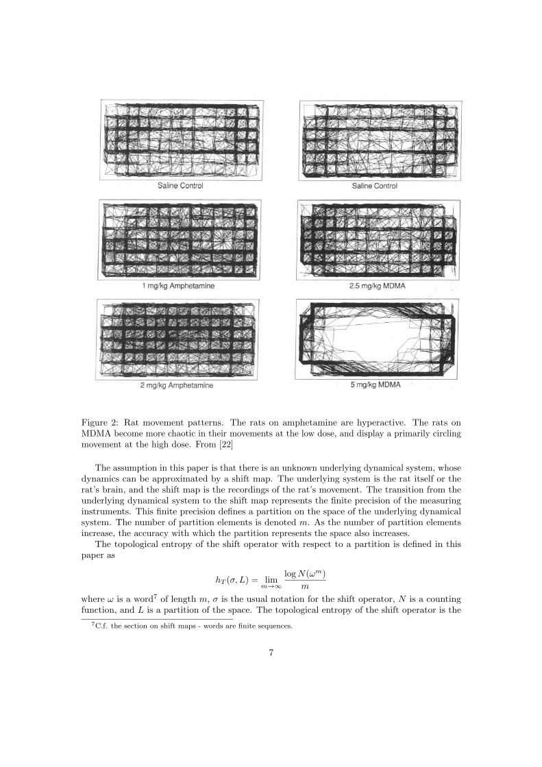
In this paper [22], rats are given different psychoactives: MDMA, amphetamines. The movementof the rats in a bounded space is converted into symbolic sequences, and the topological entropyand measure entropy are calculated for the sequence. The measurable dynamical system consistsas always of a space, a σ-algebra, a measure, and a transformation. The space is the set of infinitesequences of symbols. The σ-algebra is that generated by cylinder sets on the space; i.e., foreach finite symbol sequence, the cylinder set is the set of infinite sequences that agree with thefinite one on its set of indices. The sequences must be taken to be infinite for the entropy to benon-zero, even though in laboratory conditions the movements of the rats are only observed forfinite time. The finite observation is part of one of the infinite cylinders in the mathematicalspace. The transformation is the shift operator, which gives the time evolution. The attractoronto which the shift operator eventually maps the sequences, is the characteristic movementpattern induced by the psychoactives.

6

Figure 2: Rat movement patterns. The rats on amphetamine are hyperactive. The rats onMDMA become more chaotic in their movements at the low dose, and display a primarily circlingmovement at the high dose. From [22]

The assumption in this paper is that there is an unknown underlying dynamical system, whosedynamics can be approximated by a shift map. The underlying system is the rat itself or therat’s brain, and the shift map is the recordings of the rat’s movement. The transition from theunderlying dynamical system to the shift map represents the finite precision of the measuringinstruments. This finite precision defines a partition on the space of the underlying dynamicalsystem. The number of partition elements is denoted m. As the number of partition elementsincrease, the accuracy with which the partition represents the space also increases.

The topological entropy of the shift operator with respect to a partition is defined in thispaper as

hT (σ, L) = limm→∞

logN(ωm)

m

where ω is a word7 of length m, σ is the usual notation for the shift operator, N is a countingfunction, and L is a partition of the space. The topological entropy of the shift operator is the

7C.f. the section on shift maps - words are finite sequences.

7

supremum over partitions L of hT (σ, L). This describes the number of new sequences occuringwith increasing sequence length. The topological entropy is the growth rate of the number ofpossible words with increasing word length, considering all possible partitions8 of the measurespace. A measure entropy is also defined as the limiting average of the measure entropy withrespect to a partition L, where the measure gives a weighting of which words are more probable:

hm(σ, L) = limm→∞

H(ωm)

m

The partition could have been defined in terms of movements easily expressed in language: apoking of the head could have been one partition element, a decrease in speed could have beenanother. Instead, the authors define partition elements that are inversely proportional to thedensity distribution of points. They call this a relative generator, as opposed to a generatingpartition. The idea here is that the partition should not be specified a priori, and should be chosenrelative to its significance with respect to the data. The consequence here is that a single partitionelement may consist of a combination of poking, rearing, or acceleration movements. Subsets ofthe measure space in which the rat is observed more frequently are resolved into more distinctbehavioral events than in subsets observed less frequently. The number of partition elements isset to 32 as this seemed to saturate both the entropy creation and the largest Lyapunov exponent.

The actual probability for the different movement sequences is estimated by observing theactual rat movements. These probabilities retroactively assign a measure to the system: themeasure of a sequence is defined to be its probability. Transitions between words are written asan incidence matrix, and the probabilities transform this into a transition matrix. The Ruelle-Perron-Frobenius Theorem is used to estimate the largest Lyapunov exponent. The incidencematrix is used to calculate the largest Lyapunov exponent as well as the topological entropy. Themeasure entropy with respect to a partition is estimated as a conditional probability of one wordgiven another word with the same length:

H(ωm) ≈∑i,j

P (ωmi )[P (ωmi |ωmj ) log(Pωmi |ωmj )].

Amphetamine was observed to increase the amount of activity, leading Lyapunov exponent,topological entropy, and measure entropy in a dose-dependent fashion. The increase in transitionswas both due to an increase in spatial activity (variety of paths) as well as temporal activity(slowing down and speeding up).

The MDMA results were more complicated, as they were not dose-dependent. As the dose ofMDMA was increased, the leading Lyapunov exponent, topological entropy, and measure entropyfirst increased, and then decreased. In other words, these ergodic quantities have a biphasic,dose-dependent response to MDMA.

On closer inspection, it was observed that individual animals responded differently to highdose MDMA. At high doses, some individuals experience a decrease of ergodic quantities to thelevel of saline controls, whereas for others the ergodic quantities continue to increase. In the lowentropy response animals, there was greater topological entropy relative to measure entropy: thisindicates a decrease in the number of likely paths, in addition to a decrease in the number ofpossible paths.

The amphetamine results are compared to the Lyon-Robbins hypothesis, which states thatthe stimulant action of amphetamine causes an increase in the initiation of behavioural sequencesas well as a disruption in the completion of the sequences, eventually resulting in stereotypy.In the experiment, an increased initiation of behavioural responses corresponds to an increase

8In the context of a shift map, a partition may also be referred to as a coding.

8

of transitions between different sequences of the measure space, resulting in an increase in theleading Lyapunov exponent: an animal starts specific sequences of behavioural events and shortlythereafter initiates a new sequence. This decreased correlation of consecutive events is consistentwith the Lyon-Robbins hypothesis.

With regards to MDMA, convergence at sufficiently high doses of all animals to the lowtopological entropy and still lower measure entropy state indicates a perturbation of the centralnervous system that yields very constrained sequences of behaviour.

The paper concludes with the speculation that healthy functioning may consist in constrainedrandomness, characterised by having many possible response options available (hT ) while choosingonly a limited subset of these options (hm).

3.3 Dynamical entropy is conserved during cocaine-induced changesin fetal rat motor patterns (1996)

This paper [26] proposes that entropy is a conserved property in biological systems such as thebrain and heart. It describes an experiment suggesting that cocaine redistributes entropy.

A lost variety theory of stimulant drug action is that drugs such as cocaine induce a pathologicalsimplification of the system’s dynamics via the loss of entropy. This paper challenges this view,stating that entropy is in fact conserved, and that its redistribution is what causes damaging effects.This redistribution consists in an increase in the amount of activity, associated with a decrease inthe variety of behaviour. The authors relate this to a simplified version of Manning’s formula.The measure-theoretical aspects are dropped: the measure entropy is replaced by the topologicalentropy, and the unique positive Lyapunov exponent of a two-dimensional hyperbolic systemis replaced by the leading Lyapunov exponent. The measure-dependent Hausdorff dimension isreplaced by the correlation dimension. This gives:

hT ≈ λ1DR

The original theorems of Pesin and Manning are proved with mathematical conditions, suchas uniform expansivity, that are unrealistic for biological systems. Manning’s formula is onlyvalid for a two-dimensional system, and the substitution of the correlation dimension for theHausdorff dimension is not mathematically clear. The authors of this paper nevertheless deriveexperimental results from the approximate formula that seem meaningful.

The substance of the paper is an experiment to determine the topological entropy (dynamicalcomplexity) of fetal rats injected with cocaine. The rats are visually observed for 20 minutes,during which motor activity is verbally reported for entry into a computer. The events are thensummed and averaged into five second bins, giving 240 data points per subject.

The paper notes that a finite length biological time series is typically never long enough togive a stable estimate of the quantities9 hT , λ1, or DR. In other words, the asymptotic stabilityof these quantities cannot in practice be reached from individual time series. The number of datapoints needed to correctly estimate DR in a d-dimensional system is between 10d/2+1 and 10d. Ifthe dimension is for example six, the observation would have to last for weeks or months, farlonger than the duration of action of an injection of cocaine. Eckmann and Ruelle10 emphasisethat beyond having a large number of measurements, what matters is to have a long recordingtime - increasing the resolution of one’s measurements at fixed recording time does not help muchin capturing the dynamics. Increasing the resolution merely gives more and more information on

9Here and elsewhere, researchers in the applied sciences refer to quantities which characterise the dynamics asmeasures. This is a different use of terminology from measures in the sense of measure theory. I keep with theterm quantity to avoid confusion.

10Lyapunov exponents from time series, page three.

9

smaller and smaller pieces of the attractor, whereas one would like to let the recording time tendto infinity to reconstruct all of the attractor. The authors assert that their recording time is longenough.

To get a good estimate of hT , λ1, and DR, a spatial average over individuals is taken in placeof a single long time series of a single individual. Doing this assumes that the system of fetal ratsunder the influence of cocaine is ergodic.

A partition of the space is made by defining six partition elements as being from one to threestandard deviations above or below the mean. Each partition element corresponds to a type ofrat motor activity. A six-times-six transition matrix follows the orbits of the data points fromone partition to the next, each entry representing the probability of transition as a real number.The transition matrix is converted to an incidence matrix by replacing each entry by a 0 or 1according to the rule that a transition matrix entry of less than 0.0375 gives a 0, i.e. if thecell was visited nine times or less (9/240 = 0.0375). The asymptotic growth rate of the traceof the incidence matrix estimates its largest eigenvalue. The Ruelle zeta function11 makes anappearance, but I am not sure in what capacity.

The evolution of the separation between two neighbouring data points after five time stepswas calculated for various neighbouring pairs, the greatest rate of separation giving λ1. Thisgives a logarithmic estimate of the largest rate of expansion of new motion patterns.

The correlation dimension12, DR, is a measure of the dimensionality of the space occupied bya set of points. In statistical mechanics, the correlation function of a time series is the averagedistance between any two points xi and xj .

c(l) = limN→∞

1

N2

N∑i,j=1

i 6=j

Θ(l − ||~x(i)− ~x(j)||), ~x(i) ∈ Rm

This gives the number of pairs of data points whose distance is less than l. The correlationintegral is the integral from 0 to l of the correlation dimension with m degrees of freedom, andrepresents the mean probability that the states at two different times are close.

C(l) =

∫ l

0

dmr c(r)

C(l) is proportional to a power of l, lν . ν is the correlation dimension, and is a lower boundof the Hausdorff dimension. In this paper, the authors choose m = 5 and graphically estimate νas l goes to zero.13

The experimental results are that hT is not correlated with λ1 or DR, and that there isan inverse correlation between λ1 and DR. With administration of cocaine, the topologicalentropy remained stable, the leading Lyapunov exponent increased, and the correlation dimensiondecreased. This is given as evidence that topological entropy is conserved.

The paper states that the frequently used applied dynamical systems procedure of comparingto a random data set is irrelevant to the statistical discrimination of quantities from experimentallydefined states.

11A zeta function is a complex function that’s like a generating function. You’ve got a bunch of numbers, andrather than writing down all these numbers you can just encode them into a single function. Complex functionshave infinitely many coefficients, and all this information can be collected together in a single function. If youknew everything about the complex function you could read off all the numbers. Knowing some information aboutthe complex function can tell you some broad properties. It’s a convenient device. Zeta functions typically countperiodic behaviour.

12See Grassberger and Procaccia’s paper Measuring the strangeness of strange attractors.13They denote ν as DR and l as r.

10

Extrapolating from the experimental results to the human psychological level, an increasein the leading Lyapunov exponent corresponds to increased busyness, while the concomitantdecrease in the correlation dimension corresponds to reduced degrees of freedom in thought andbehaviour. This is the profile of the complexity-conserving obsessive-compulsive or workaholicpersonality. The paper suggests that this loss of complexity can be just as damaging as thesupposed entropy reduction of the alternative lost variety theory.

3.4 Intermittent Vorticity, Power Spectral Scaling, and DynamicalMeasures on Resting Brain Magnetic Field Fluctuations (2011)

This [17] is a pilot study on resting state MEG data from 10 schizophrenics and 10 controls. Oneview of resting state MEG data is that it is background noise. This view is more typical of sourcelocalisation studies of task-related MEG data. The authors take the alternative view that restingstate MEG data is physiologically and psychologically relevant.

In studies of functional networks of brain regions, resting state activation is sometimes referredto as the Default Mode Network (DMN). The DMN is a spatial characterisation of resting stateactivity, and is observed via fMRI scans which have high spatial resolution and low temporalresolution. The authors of this pilot study use MEG scans which have a much higher temporalresolution, in view of a temporal characterisation of resting state activity.

The authors mention how neuroscientists such as Michael Greicius have suggested that restingstate activity reflects task-unrelated images and thoughts. These task unrelated thoughts (TUT)have also been referred to as daydreaming or stimulus independent thoughts (SIT), and I willrefer to them as the thinking mind, as opposed to the task-oriented working mind. The authorsmention evidence that the thinking mind persists under anesthesia.

The data examined is 12.5, 54, 180 or 240 seconds of eyes closed, resting spontaneous magneticfield activity in ten resting controls and ten medicated schizophrenics. The measurable entropymanifold volume (MEMV) is defined as the product of the topological entropy, leading Lyapunovexponent, and capacity dimension. The authors state that this is a three-dimensional entropyvolume measure, but I am unclear on how this can represent a volume. Capacity dimension isunitless, and entropy and Lyapunov exponents have units of inverse time, suggesting that MEMVis an acceleration.

Prominent magnetic field fluctuations, which the paper title refers to as vorticity, are referredto in the paper as strudels. The paper speculates that strudels are the thinking mind and thatMEMV represents what might be called psychic energy or psychic entropy. The hypothesis isthat MEMV is used up in the generation of strudels.

A common paradigm for MEG is the inverse problem: reconstructing the orientation andlocation of magnetic dipoles needed to produce a given a MEG. The inverse problem is underde-termined, in that many dipole configurations may produce the same MEG. This paper insteadattempts to analyse the MEG globally, by analysing the sequences of differences between twobilaterally symmetric sensor pairs, and refers to this as the symmetric sensor difference sequence(SSDS). Seeking to disprove the assumption that local polarities of the magnetic field cancel out,the SSDS is designed to show that a seed magnetic fluctuation can diffuse across spatiotemporalscales.

A three minute SSDS signal has 144,000 data points. Some unknown function Φ acting onthe SSDS is the time evolution of the underlying dynamical system. Singular spectrum analysisof the signal is used to estimate the leading eigenfunction14 of the SSDS, written Ψ1. This isdone by using the method of delays to create a covariance matrix where each row is a delay ofthe SSDS time series. The leading eigenvector given by singular spectrum analysis is calculated

14An eigenfunction is an eigenvector that is also a function.

11

at each point of the SSDS to give the leading eigenfunction, which the authors call the leadingBroomhead-King eigenfunction.

When analysing something, it can be useful to break it up into its component frequencies, justas white light is made up of colours which each have their own frequency. A Fourier transformanalyses frequency from the perspective of eternity, and misses out on how the frequency changeswith time. The short time Fourier tranform uses a window function to catch the frequencycomponent in a time interval, but it can miss out on some information by having a window that’stoo long or too short, like glasses that are not adapted to one’s eyesight. By a kind of uncertaintyprinciple, the product of the time resolution and the frequency resolution is constant. A wavelettransform takes advantage of this by having a window with varying width, allowing it to see bothshort duration high frequency information as well as long duration low frequency information.

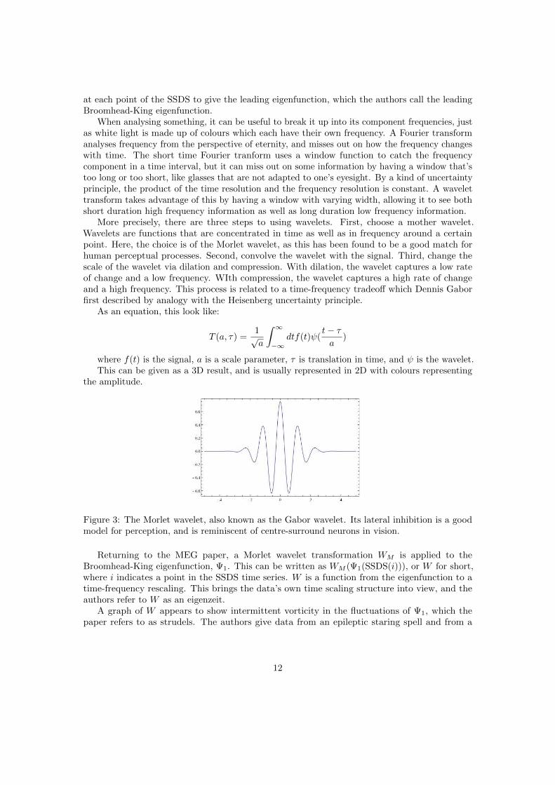
More precisely, there are three steps to using wavelets. First, choose a mother wavelet.Wavelets are functions that are concentrated in time as well as in frequency around a certainpoint. Here, the choice is of the Morlet wavelet, as this has been found to be a good match forhuman perceptual processes. Second, convolve the wavelet with the signal. Third, change thescale of the wavelet via dilation and compression. With dilation, the wavelet captures a low rateof change and a low frequency. WIth compression, the wavelet captures a high rate of changeand a high frequency. This process is related to a time-frequency tradeoff which Dennis Gaborfirst described by analogy with the Heisenberg uncertainty principle.

As an equation, this look like:

T (a, τ) =1√a

∫ ∞−∞

dtf(t)ψ(t− τa

)

where f(t) is the signal, a is a scale parameter, τ is translation in time, and ψ is the wavelet.This can be given as a 3D result, and is usually represented in 2D with colours representing

the amplitude.

Figure 3: The Morlet wavelet, also known as the Gabor wavelet. Its lateral inhibition is a goodmodel for perception, and is reminiscent of centre-surround neurons in vision.

Returning to the MEG paper, a Morlet wavelet transformation WM is applied to theBroomhead-King eigenfunction, Ψ1. This can be written as WM (Ψ1(SSDS(i))), or W for short,where i indicates a point in the SSDS time series. W is a function from the eigenfunction to atime-frequency rescaling. This brings the data’s own time scaling structure into view, and theauthors refer to W as an eigenzeit.

A graph of W appears to show intermittent vorticity in the fluctuations of Ψ1, which thepaper refers to as strudels. The authors give data from an epileptic staring spell and from a

12

schizophrenic thought blocking15 episode. In both cases the subjective experience is of beingunable to form thoughts, and the W graphs are of a sudden absence of strudels. MEMV alsoappears to be reduced by 40-50% in schizophrenics versus controls.

Figure 4: Morlet wavelet transformation of the leading eigenfunction of the SSDS of left and rightC16 sensors. From bottom to top, there seem to be small scale fast driving events, intermediatescale 1-3 Hz waves, and the intermittent emergence of longer strudels from some but not all fastand intermediate scale events. From [17]

15The schizophrenic thought blocking data appears in their later paper Daydreaming, Thought Blocking andStrudels in the Taskless, Resting Human Brain’s Magnetic Fields. Thought blocking occurs when a person’s speechis suddenly interrupted by silence that lasts for a few seconds or minutes. It is often brought on in schizophrenicsby discussing something emotionally heavy, and is described as a quick and total emptying of the mind.

13

4 MEG Time Series Analysis

79 resting state MEG recordings lasting four minutes each are studied to assess the entropy levelin the left and right hemispheres. The recordings are from controls, medicated schizophrenics,and unaffected siblings of schizophrenics.

This analysis assumes that the MEG is deterministic rather than stochastic. It considers theMEG time series as representative of an underlying deterministic dynamical system.

First, the data is imported into MATLAB using the EEG/MEG FieldTrip toolbox. Then, Iselect pairs of sensor channels from each hemisphere from the imported dataset. The channels Istudy are left and right C16 (central), left and right P57 (parietal), and left and right F14 (frontal).The sensor map is that of CTF’s 275 lead MEG scanner. Fieldtrip’s CTF275.lay file provides thecorrespondence between label and layout. To cancel noise, the time series is subtracted for twosensors on the same hemisphere: for example, one time series is formed from the right C16 timeseries from which the right P57 time series has been subtracted. This is similar to the SSDS inthe previous section, except that the sensor difference sequence is no longer symmetric, since thetwo sensors are now from the same hemisphere. In this way six pairs of channels form six timeseries, three for each hemisphere. The primary purpose of taking more than one pair is to guardagainst possible noise at a particular channel location, rather than to distinguish between regionswithin a given hemisphere. Finally, I run custom MATLAB functions on the new time series andassess the hemisphere-specific differences. The functions are adapted from the Simple Aggregatefor Nonlinear Time-series Analysis project16 (SANTA), which I am currently helping to renovate.

16http://vlsi-cuda.ucsd.edu/~braindyn/index.php

14

Figure 5: Sensor locations. From [17]

4.1 Viewing the data in MATLAB with the FieldTrip toolbox

This example MEG file was recorded using the CTF MEG System17. The dataset is stored ina .ds folder, in this case one for each subject. FieldTrip functions are used to read the headerinformation and to read the data into a matrix.

cfg.dataset = 'Subject 01.ds';

hdr = ft read header('Subject 01.ds')

hdr =

Fs: 600 % sampling frequency

17www.ctfmeg.com/index.html

15

nChans: 332 % number of channelsnSamples: 144000 % number of samples per trial

nSamplesPre: 0 % number of pre-trigger samples in each trialnTrials: 1 % number of trials

label: {332x1 cell} % cell-array with labels of each channelgrad: [1x1 struct] % gradiometer structureorig: [1x1 struct] % additional header information

chantype: {332x1 cell} % type of data of each individual channelchanunit: {332x1 cell} % physical units of each channel

dat = ft read data('Subject 01.ds');

format long e

unit = ft chanunit(hdr)

The header data structure contains a vector, hdr.label, which associates each line index withthe corresponding sensor of the MEG scanner. The FieldTrip function ft chanunit gives the unitsof the MEG data. The first row is time in seconds, and the remaining rows are magnetic fieldstrength in tesla. The format command changes the display precision so that the tesla values donot all show as zeros.

Here is the beginning of the first two columns of MEG data.

>> dat(:,1:2)

ans =

8.337461750000000e+03 8.337463416666666e+03-1.385906494693436e-09 -1.387690267455668e-092.241682167274993e-09 2.240907212037669e-09-4.404843752375973e-09 -4.401568073661994e-091.778295613667668e-09 1.776501210481651e-09-1.662896100804182e-10 -1.681567006944026e-10-3.829996110958704e-09 -3.826533741538616e-093.635103659536867e-10 3.628395726104604e-103.055356748903700e-09 3.053415729348467e-09

Both the header data and the first row of the MEG data indicate that the MEG is sampled atthe millisecond scale. In the MEG data, the digits 8.33746e+03 remain the same in the first andsecond timestep, corresponding to 8337.46 seconds or 833746 centiseconds.

MEG magnetic field strength is measured in thousands of femtotesla, 10−12 − 10−11 T. Afemtotesla is 10−15 T, and the magnetic field generated by the heart is on the order of a nanotesla,10−9 T. Taking the difference of two sensors allows for cancellation of noise.

4.2 Topological entropy and measure entropy

For a description of topological and measure entropy, see my essay mentioned in the introduction.Recall that the topological entropy is an upper bound to the entropy with respect to any measure.

hµ ≤ hTAn incidence matrix represents which transitions occur in a partition space of the time series.

The topological entropy is estimated as the logarithm of the maximum eigenvalue of the incidencematrix.

A transition matrix estimates the probability of going from one partition to another withinthe time series. If the system is ergodic, one can find the asymptotic probability distribution -

16

in other words, one can find the natural measure corresponding to the underlying measurabledynamical system. This allows for calculation of the measure entropy.

Below is the code used to calculate the topological entropy and measure entropy. I haveincluded a lot of commentary directly in the code to explain how the calculation works.

Note that the implementation of the measure entropy is not complete - at the moment thiscode only calculates the topological entropy, as well as the average information18 which is a stepto calculating the measure entropy.

The time series points are allocated box indices in a high-dimensional embedding space. Iused an 11 dimensional embedding space with 4 partitions per dimension. The high embeddingspace dimension is made possible by the use of sparse matrices. Once the partition indices arechosen, a transition matrix is formed, and simplified into an incidence matrix. The topologicalentropy is estimated as the logarithm of the maximum eigenvalue of the incidence matrix.

function [topologicalEntropy, measureEntropy] = CalcEntropySparse(timeSeries, ...embeddingDimension, partitionsPerDimension)

% CalcEntropySparse(timeSeries, embeddingDimension, partitionsPerDimension)%% Calculates the Topological and Measure Entropies%% Parameters: timeSeries - The time slice of data to be analyzed, as a row% vector embeddingDimension - The embedding dimension% partitionsPerDimension - The number of partitions in each dimension%% Return: topologicalEntropy - The Topological Entropy measureEntropy - The% Measure Entropy%% Description: Calculates the Topological and Measure entropies, first% finding the sparsity pattern so as to optimise memory usage. An embedding% dimension of 2d+1 can reconstruct an attractor of dimension d. For% analysing the EEG or MEG, if the attractor is assumed to be eight, this% requires a seventeen dimensional embedding space, which requires a lot of% memory. Topological entropy is found as the logarithm of the maximum% eigenvalue of the incidence matrix formed from the time series. The% incidence matrix is composed of 1s and 0s, and indicates whether a% transition from one partition to another occurs. Measure entropy is found% with respect to the measure induced by the probabilities of the% transition matrix formed from the time series. The transition matrix, or% Markov matrix, gives the probabilities for going from one partition to% another. This allows the data to produce its own measure, the natural% measure (also know as the Sinai-Ruelle-Bowen measure or physical% measure).%% The embedding space is covered with partitions, with the number of% partitions per dimension and the number of dimensions of the embedding% space given by the input parameters. The partitions are then labeled.% Imagine a single dimension partitioned into 4 partitions, with values% normalized between 0 and 1. This means that anything between 0 and 0.25% is partition 1, anything between 0.25 and 0.5 is partition 2, and so on.% But then imagine pulling it out into 2 dimensions and now the partitions% are squares. Then the first row of squares is 1 through 4 and the next% is 5 through 8 and so on. The box number that the point lies in is% dependent on it's value in the first and second dimensions. Moving it% along the second dimension changes its box number by 4 each time and% moving it along the first dimension changes the box number by 1. In

18This is H, capital H, in the discussion of measure entropy in my aforementioned essay.

17

% three dimensions the partition moves up a plane (16 boxes) so the box% number changes by 16. In this way a number is assigned to every% partition.%% Topological entropy is an upper bound to measure entropy.%% WARNING: there is a known bug with this code where the entropies given% are complex values. Re-run the code with the same inputs until you get% real outputs. This problem may be caused by the instability of Matlab's% eigenvalue calculation algorithm.

data = timeSeries'; %has to be a column vector for accumarray later on

%nBox is the total number of partitions (also known as boxes or hypercubes)%covering the embedding dimension.nBox = partitionsPerDimensionˆembeddingDimension;

mn = min(data); %minimum value of the time seriesmx = max(data); %maximum value of the time seriesmx = mx + 1e-6*(mx - mn);%small offset to the boundary of the rightmost partition to make sure that%the maximum data point is included in the last partition

%restructure the data array to convert it to linear partition indices; the%idea is to reshape the data into a table, where each successive column is%the data sequence delayed by a successive delay; there is a Matlab%command, delayseq, which could be used for this, but it doesn't come with%the default Matlab licenselags = (0:(embeddingDimension - 1)) + 1; %index (into data array) of the first ...

entry in each columnflp lags = fliplr(lags) - 1; %offset from end of data array for each columndataToPartitionIndex = zeros(length(data) - flp lags(1), embeddingDimension); ...

%preallocate memoryfor i = 1:embeddingDimension

dataToPartitionIndex(:, i) = data(lags(i):(end - flp lags(i)));end%each column of dataToPartitionIndex is a delayed copy of the time series;%the first column has no delay, the second column has a delay of 1, and so%on up to (embeddingDimension - 1)

%preallocating memory by initialising the incidence and transition matrices%to zeros uses too much memory when nBox is very large

%Instead of working wth matrices straight away, first find the%sparsity pattern, i.e. the indices of the non-zero entries in the%matrices and the values that go into these entries

%the bsxfun command can subtract and multiply%matrices by vectors i.e. each row of a matrix gets combined with a row%vectorpartitionRange = (mx - mn)/partitionsPerDimension;%mx-mn is the range of the data, and dividing this by%partitionsPerDimension gives the range of the partition along any given%dimensiondataToPartitionIndex = fix((dataToPartitionIndex - mn)/partitionRange);%subtracting the minimum gives the distance of the data point from the%minimum; Normalizing by partitionRange contains the values between 0 and%the number of partitions ; normalizing by the range only would contain the%values between 0 and 1

%at this stage dataToPartitionIndex is an array of partition subscripts;%each column contains values in [0, nPart - 1] since we want to represent

18

%the transitions between partitions in a square matrix form (the transition%and incidence matrices), we want to convert the partition subscripts into%a single number: the linear indexdataToPartitionIndex = bsxfun(@times, dataToPartitionIndex, ...

partitionsPerDimension.ˆ(0:(embeddingDimension - 1)));%first step towards linear indices; see the description of partition%numbering in the introductiondataToPartitionIndex = sum(dataToPartitionIndex, 2) + 1;%second step towards linear indices; now dataToPartitionIndex is a single%column of linear partition indices for the time series points

%look at the transitions between partitions: create an array of transitions%from one partition to the next partitiondataToPartitionIndex = [dataToPartitionIndex(1:(end - 1)), ...

dataToPartitionIndex(2:end)];

%At this point we pretty much have the sparsity pattern, except for the%following possibilities% we may have partitions which are never visited. we may also have% partitions which can be entered, but never exited we may also have% partitions which are exited, but never entered%these conditions would imply that the Markov chain representation is not%irreducible which means it's not going to have a stationary distribution%we have to eliminate such possibilities for the below code to work

%first let's ignore the diagonal matrix entries for now i.e. let's ignore%the transitions from every state i to itselfoff diag = dataToPartitionIndex; %copy the transition listoff diag(off diag(:, 1) == off diag(:, 2), :) = []; %remove entries where both ...

columns hold the same index

%if a state index is present in both columns of off diag, then it must be%both enterable and exitableenterable = false(nBox, 1);exitable = enterable;exitable(off diag(:, 1)) = true; %marks partitions which have at least one outgoing ...

transitionenterable(off diag(:, 2)) = true; %marks partitions which have at least one ...

incoming transitiondelete partitions = ~(enterable & exitable); %if not both enterable and exitable, ...

the partition must be removed%delete partitions also marks partitions which are never visited

%for the transition matrix, we want to count the number of transitions%and put the number into the correct matrix entry; notice how the issparse%argument to accumarray is set to true, so that the output is a sparse matrixtransitionMatrix = accumarray(dataToPartitionIndex, 1, [nBox, nBox], [], [], true); ...

%transition count

%remove the marked partitions from the matrixtransitionMatrix(delete partitions, :) = []; %delete the corresponding rowstransitionMatrix(:, delete partitions) = []; %delete the corresponding columns

%normalise the rowstransitionMatrix = spdiags(sum(transitionMatrix, 2), 0, size(transitionMatrix, 1), ...

size(transitionMatrix, 1))\transitionMatrix;

%the stationary distribution is the principal left eigenvaule of the%transition matrix; for sparse matrices we use the command eigs() to get the%right eigenvectors; since we want left, not right eigenvectors, we have to%transpose the matrix before taking eigenvectors[right eig vectors, ~] = eigs(transitionMatrix'); %calculate right eigenvalues of ...

19

transposed matrixrw = right eig vectors(:, 1); %first right eigenvalue corresponds to stationary ...

distribution

%we now normalise the eigenvector and calculate the entropy of the%stationary distributionnzr = rw ~= 0; %ignore states with zero probability, this should never occur since ...

we've made sure our Markov chain has a stationary distributionrw = rw(nzr)./sum(rw(nzr)); %normaliseaverageInformation = sum(-rw(nzr).*log(rw(nzr)));%the measure entropy of the stationary distribution is obtained by iterating the ...

average information over sequence length - Not implemented yet!

%for the topological entropy matrix, we want to simply have a non-zero%entry for every transition which has occured in the time series. So we just%want the non zero entries of the measure entropy matrixincidenceMatrix = double(transitionMatrix > 0);

%the logarithm of the maximum eigenvalue of the incidence matrix estimates%the topological entropyeigtemp = eigs(incidenceMatrix);topologicalEntropy = log(max(abs(eigtemp)));end

4.3 Results

All subjects except three had higher topological entropy in the right hemisphere of the restingstate MEG. With a higher ratio indicating more entropy in the right hemisphere, the averageentropy ratio for medicated schizophrenics was 1.5584, 1.5441 for unaffected siblings, and 1.6497for control subjects. Of the three subjects with dominant left hemisphere topological entropy,one was a medicated schizophrenic, one a control, and one an unaffected sibling.

Performing a simple one-sample t-test on the null hypothesis that entropy is equally distributedin left and right hemispheres, i.e. that the ratio is 1, without differentiating between schizophrenics,siblings and controls, it is found that the average is significant (with a p-value lower than 0.00001).This is therefore evidence that entropy is not equally distributed between right and left hemispheresin humans.

Differentiating between the groups, I have tested the hypothesis that schizophrenics havea different entropy ratio, compared to non-schizophrenics. To test this, I have taken out theobservations of the siblings: they are not statistically independent of the schizophrenics. I haveassumed that the entropy ratio is a normally distributed variable, like other human physicalcharacteristics such as height and weight. This allows for testing even though one of the groups -the medicated schizophrenics - is small - less than 30. The hypothesis is tested by means of atwo-sample t-test as follows. First I compute the sample variation of the test statistic.

SE =

√S21

n1+S22

n2

S1 and S2 are the variances of the sample of medicated schizophrenic entropies and controlentropies, respectively. Here S1 = 0.0560 and S2 = 0.0554. n1 and n2 are the sizes of the sampleof medicated schizophrenic group and control group, respectively. Here n1 = 21 and n2 = 44.

Then I determine the degrees of freedom, assuming that the variances of the two populations(schizophrenics and controls) are different.

20

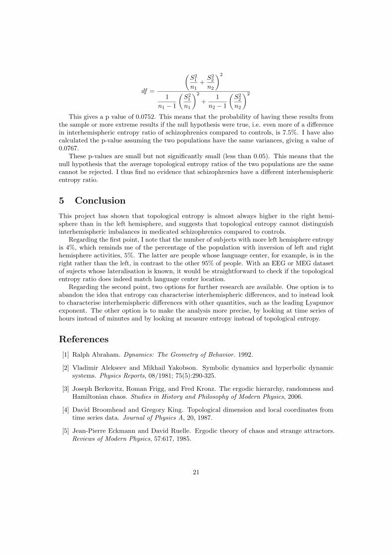
df =

(S21

n1+S22

n2

)2

1

n1 − 1

(S21

n1

)2

+1

n2 − 1

(S22

n2

)2

This gives a p value of 0.0752. This means that the probability of having these results fromthe sample or more extreme results if the null hypothesis were true, i.e. even more of a differencein interhemispheric entropy ratio of schizophrenics compared to controls, is 7.5%. I have alsocalculated the p-value assuming the two populations have the same variances, giving a value of0.0767.

These p-values are small but not significantly small (less than 0.05). This means that thenull hypothesis that the average topological entropy ratios of the two populations are the samecannot be rejected. I thus find no evidence that schizophrenics have a different interhemisphericentropy ratio.

5 Conclusion

This project has shown that topological entropy is almost always higher in the right hemi-sphere than in the left hemisphere, and suggests that topological entropy cannot distinguishinterhemispheric imbalances in medicated schizophrenics compared to controls.

Regarding the first point, I note that the number of subjects with more left hemisphere entropyis 4%, which reminds me of the percentage of the population with inversion of left and righthemisphere activities, 5%. The latter are people whose language center, for example, is in theright rather than the left, in contrast to the other 95% of people. With an EEG or MEG datasetof sujects whose lateralisation is known, it would be straightforward to check if the topologicalentropy ratio does indeed match language center location.

Regarding the second point, two options for further research are available. One option is toabandon the idea that entropy can characterise interhemispheric differences, and to instead lookto characterise interhemispheric differences with other quantities, such as the leading Lyapunovexponent. The other option is to make the analysis more precise, by looking at time series ofhours instead of minutes and by looking at measure entropy instead of topological entropy.

References

[1] Ralph Abraham. Dynamics: The Geometry of Behavior. 1992.

[2] Vladimir Alekseev and Mikhail Yakobson. Symbolic dynamics and hyperbolic dynamicsystems. Physics Reports, 08/1981; 75(5):290-325.

[3] Joseph Berkovitz, Roman Frigg, and Fred Kronz. The ergodic hierarchy, randomness andHamiltonian chaos. Studies in History and Philosophy of Modern Physics, 2006.

[4] David Broomhead and Gregory King. Topological dimension and local coordinates fromtime series data. Journal of Physics A, 20, 1987.

[5] Jean-Pierre Eckmann and David Ruelle. Ergodic theory of chaos and strange attractors.Reviews of Modern Physics, 57:617, 1985.

21

[6] Jean-Pierre Eckmann, David Ruelle, Sergio Ciliberto, and Sylvie Oliffson Kamphorst. Lya-punov exponents from time series. Physical Review A, 1986.

[7] Roman Frigg, Joseph Berkovitz, and Fred Kronz. http://plato.stanford.edu/entries/ergodic-hierarchy. 2011.

[8] Peter Grassberger and Itamar Procaccia. Measuring the strangeness of strange attractors.Physica 9D, 9:189–208, 1983.

[9] Brook Henry, Arpi Minassian, Martin Paulus, Mark Geyer, and William Perry. Heart ratevariability in bipolar mania and schizophrenia. Journal of Psychiatric Research, 44:168–176,2010.

[10] Holger Kantz. Nonlinear Time Series Analysis. 2004.

[11] Arnold Mandell. Dynamical complexity and pathological order in the cardiac monitoringproblem. Physica A: Statistical Mechanics and its Applications, 27D:235–242, 1987.

[12] Arnold Mandell. Can a metaphor of physics contribute to MEG neuroscience research?Intermittent turbulent eddies in brain magnetic fields. Chaos, Solitons & Fractals, 55:95–101,2013.

[13] Arnold Mandell, Stephen Robinson, Karen Selz, Constance Schrader, Tom Holroyd, andRichard Coppola. The turbulent human brain: An MHD approach to the MEG. 2014.

[14] Arnold Mandell and Karen Selz. Entropy conservation as HTµ ≈ λ̄+µ dµ in neurobiologicaldynamical systems. Chaos: An Interdisciplinary Journal of Nonlinear Science, 7:67–81, 1997.

[15] Arnold Mandell and Karen Selz. An intuitive guide to the ideas and methods of dynamicalsystems for the life sciences. 1998.

[16] Arnold Mandell, Karen Selz, John Aven, Tom Holroyd, and Richard Coppola. Daydreaming,thought blocking and strudels in the taskless, resting human brain’s magnetic fields. AmericanInstitute of Physics Proceedings, 2011.

[17] Arnold Mandell, Karen Selz, Lindsay Rutter, Tom Holroyd, and Richard Coppola. Intermit-tent vorticity, power spectral scaling, and dynamical measures on resting brain magneticfield fluctuations. The Dynamic Brain, 2011.

[18] Anthony Manning. A relation between Lyapunov exponents, Hausdorff dimension andentropy. Ergodic theory and dynamical systems, 1:451–459, 1981.

[19] Martin Paulus, Mark Geyer, and David Braff. Use of methods from chaos theory to quantifya fundamental dysfunction in the behavioral organization of schizophrenic patients. AmericanJournal of Psychiatry, 1996.

[20] Martin Paulus, Mark Geyer, and David Braff. Long-range correlations in choice sequences ofschizophrenic patients. Schizophrenia Research, 53:69–75, 1999.

[21] Martin Paulus, Mark Geyer, and Arnold Mandell. Statistical mechanics of a neurobiologicaldynamical system: The spectrum of local entropies applied to cocaine-perturbed behavior.Physica A: Statistical Mechanics and its Applications, 1991.

[22] Martin Paulus, Arnold Mandell, Mark Geyer, and Lisa Gold. Application of entropy measuresderived from the ergodic theory of dynamical systems to rat locomotor behavior. Proceedingsof the National Academy of Sciences, 87:723–727, 1990.

22

[23] William Perry, Arpi Minassian, Martin Paulus, Jared Young, Meegin Kincaid, Eliza Ferguson,Brook Henry, Xiaoxi Zhuang, Virginia Masten, Richard Sharp, and Mark Geyer. A reverse-translational study of dysfunctional exploration in psychiatric disorders. Archives of GeneralPsychiatry, 2009.

[24] Kevin Short. Direct calculation of metric entropy from time series. Journal of ComputationalPhysics, 104:162–172, 1993.

[25] Yakov Sinai. Introduction to ergodic theory. Princeton University Press, 1976.

[26] William Smotherman, Karen Selz, and Arnold Mandell. Dynamical entropy is conservedduring cocaine-induced changes in fetal rat motor patterns. Psychoneuroendocrinology,21:173–187, 1996.

[27] Julien Sprott. Chaos and Time-Series Analysis. 2003.

[28] Floris Takens. Detecting strange attractors in turbulence. Dynamical Systems and Turbulence,Lecture Notes in Mathematics, 898:366–381, 1981.

[29] Lai-Sang Young. What are SRB measures, and which dynamical systems have them? 2002.

23