NONLINEAR TIME SERIES ANALYSIS, WITH APPLICATIONS TO MEDICINE JosØ Mara Amig Centro de Investigacin Operativa, Universidad Miguel HernÆndez, Elche (Spain) J.M. Amig (CIO) Nonlinear time series analysis 1 / 40
Transcript
NONLINEAR TIME SERIES ANALYSIS,WITH APPLICATIONS TO MEDICINE
José María Amigó
Centro de Investigación Operativa, Universidad Miguel Hernández, Elche (Spain)
J.M. Amigó (CIO) Nonlinear time series analysis 1 / 40
LECTURE 3SYMBOLIC DYNAMICS
J.M. Amigó (CIO) Nonlinear time series analysis 2 / 40
J.M. Amigó (CIO) Nonlinear time series analysis 10 / 40
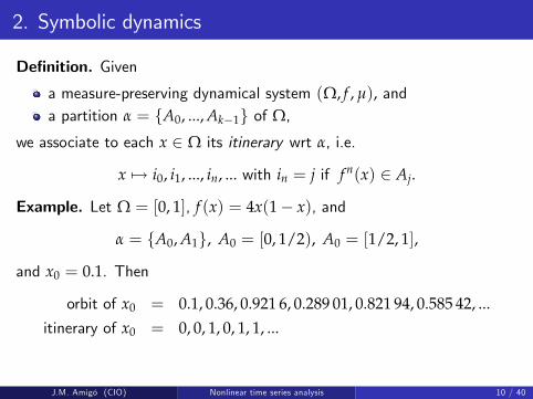
2. Symbolic dynamics
Let i0, i1, ..., in, ... be the itinerary of x wrt α = fA0, ..., Ak1g. Set
Xα(x) = i0, i1, ..., in, ... fXαn(x)gn0
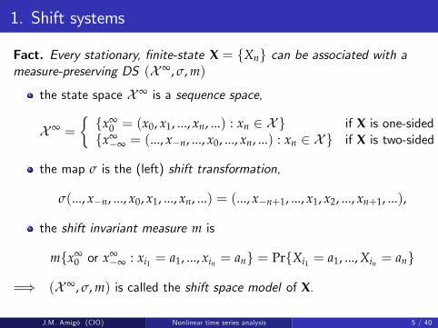
Fact. Xα is a stationary, nite-alphabet RP, X = f0, ..., k 1g, with
Pr fXα0 = i0, Xα
1 = i1, ..., Xαn = ing = µ
Ai0 \ f1Ai1 \ ...\ fnAin
.
Denition. Xα is called the symbolic dynamics of f wrt α.
If f is invertible, the itineraries and symbolic dynamics are two-sided.
J.M. Amigó (CIO) Nonlinear time series analysis 11 / 40
3. Kolmogorov-Sinai entropy
Let Xα = fXαng be the symbolic dynamics of f wrt to α = fA0, ..., Ak1g.
Denition.
The entropy of f wrt α is
hµ(f , α) = h(Xα)
The metric (or Kolmogorov-Sinai) entropy of f is
hµ(f ) = supα
hµ(f , α)
Fact. If (X∞, σ, m) is the shift space model of a random process X, then
hm(σ) = h(X).
J.M. Amigó (CIO) Nonlinear time series analysis 12 / 40
3. Kolmogorov-Sinai entropy
A partition γ of Ω is called a generating partition or a generator of f if
hµ(f ) = hµ(f , γ).
The computation of hµ(f ) is in general di¢ cult. Exceptions:
1 A generator of f is known (seldom, but there are numerical methods).2 If the invariant measure is smooth (i.e., µ(dx) = ρ(x)dx with ρdi¤erentiable), the KS entropy is the sum of the positive Lyapunovexponents (Pesins formula).
3 A closed formula is known for some maps (Bernoulli shifts, etc.)
Otherwise. Calculate hµ(f , α) for ever ner box partitions α1, α2, ..., αn, ...
limn!∞
hµ(f , αn) = hµ(f ).
J.M. Amigó (CIO) Nonlinear time series analysis 13 / 40
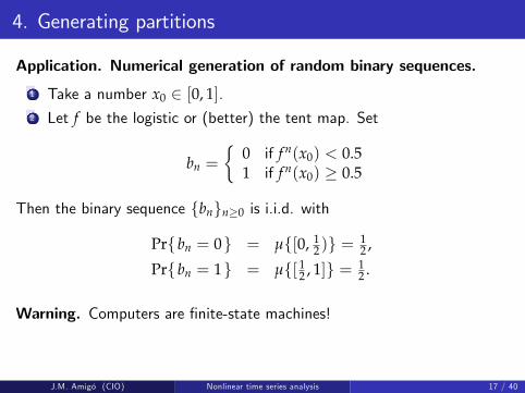
4. Generating partitions
Example. Let (X∞, σ, m) be a (p0, ..., pk1)-Bernoulli (one-sided) shiftspace. The partition γ = fC0, ..., Ck1g,
C0 = fx∞0 : x0 = 0g, C1 = fx∞
0 : x0 = 1g, ..., Ck1 = fx∞0 : x0 = k 1g
can be proved to be a generator of the shift transformation, so
hm(σ) = hm(σ, γ) = k1
∑i=0
m(Ci) log m(Ci).
J.M. Amigó (CIO) Nonlinear time series analysis 14 / 40
4. Generating partitions
Let (Ω, f , µ) be a measure-preserving dynamical system. There existgenerators of f under quite general conditions.
Fact. Let γ be a generator of f . Then
the shift space model of Xγ is an isomorphic copyof (Ω, f , µ)
J.M. Amigó (CIO) Nonlinear time series analysis 21 / 40
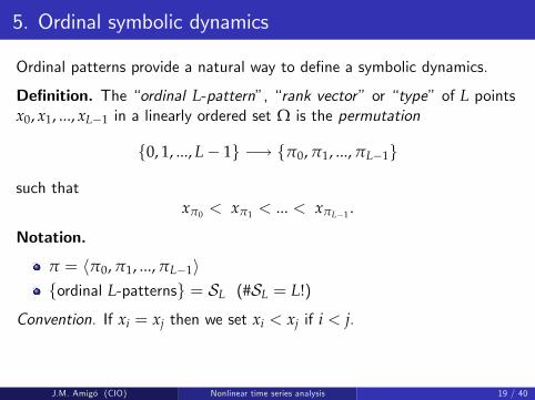
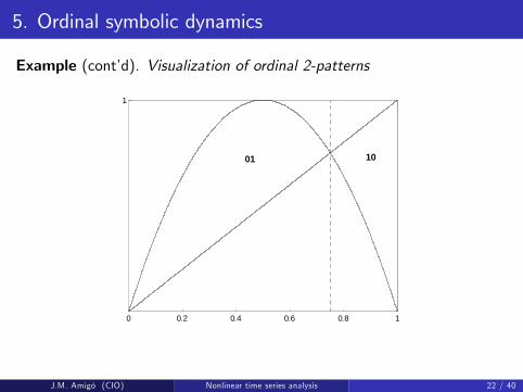
5. Ordinal symbolic dynamics
Example (contd). Visualization of ordinal 2-patterns
0 0.2 0.4 0.6 0.8 1
1
01 10
J.M. Amigó (CIO) Nonlinear time series analysis 22 / 40
5. Ordinal symbolic dynamics
Example (contd). Visualization of ordinal 3-patterns
0 0.2 0.4 0.6 0.8 1
1
012 021 201 102 120
J.M. Amigó (CIO) Nonlinear time series analysis 23 / 40
5. Ordinal symbolic dynamics
Ordinal symbolic dynamics is the symbolic dynamics which symbolsare ordinal patterns of a xed length L.The state space Ω gets divided in L! disjoint subsets Pπ, π 2 SL,namely
Pπ = fx 2 Ω : x has type π 2 SLg.The partition
PL = fPπ 6= ∅ : π 2 SLgis called the ordinal partition of Ω of length L.Use 3 L 7 in applications.
J.M. Amigó (CIO) Nonlinear time series analysis 24 / 40
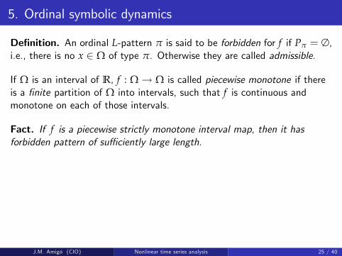
5. Ordinal symbolic dynamics
Denition. An ordinal L-pattern π is said to be forbidden for f if Pπ = ∅,i.e., there is no x 2 Ω of type π. Otherwise they are called admissible.
If Ω is an interval of R, f : Ω! Ω is called piecewise monotone if thereis a nite partition of Ω into intervals, such that f is continuous andmonotone on each of those intervals.
Fact. If f is a piecewise strictly monotone interval map, then it hasforbidden pattern of su¢ ciently large length.
J.M. Amigó (CIO) Nonlinear time series analysis 25 / 40
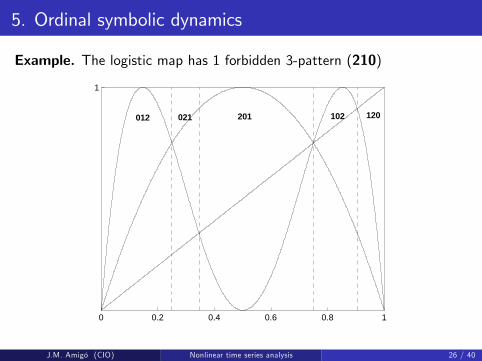
5. Ordinal symbolic dynamics
Example. The logistic map has 1 forbidden 3-pattern (210)
0 0.2 0.4 0.6 0.8 1
1
012 021 201 102 120
J.M. Amigó (CIO) Nonlinear time series analysis 26 / 40
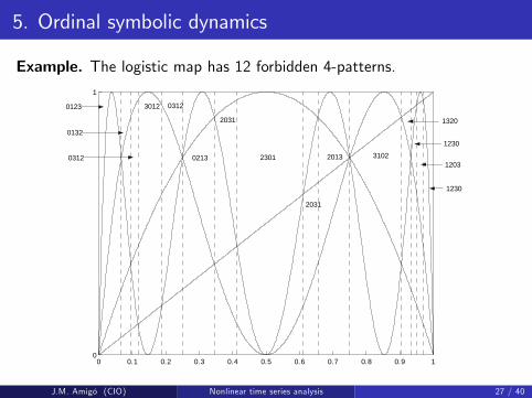
5. Ordinal symbolic dynamics
Example. The logistic map has 12 forbidden 4-patterns.
0 0.1 0.2 0.3 0.4 0.5 0.6 0.7 0.8 0.9 10
1
0123
0132
0312
3012 0312
0213
2031
2301
2031
2013 3102
1320
1230
1203
1230
J.M. Amigó (CIO) Nonlinear time series analysis 27 / 40
5. Ordinal symbolic dynamics
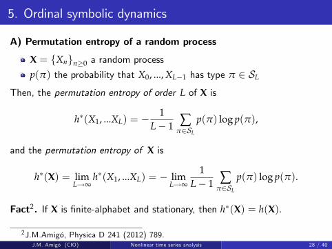
A) Permutation entropy of a random process
X = fXngn0 a random process
p(π) the probability that X0, ..., XL1 has type π 2 SL
Then, the permutation entropy of order L of X is
h(X1, ...XL) = 1
L 1 ∑π2SL
p(π) log p(π),
and the permutation entropy of X is
h(X) = limL!∞
h(X1, ...XL) = limL!∞
1L 1 ∑
π2SL
p(π) log p(π).
Fact2. If X is nite-alphabet and stationary, then h(X) = h(X).
2J.M.Amigó, Physica D 241 (2012) 789.J.M. Amigó (CIO) Nonlinear time series analysis 28 / 40
5. Ordinal symbolic dynamics
B) Permutation entropy of a dynamical system
(Ω, f , µ) a measure-preserving DS
PL = fPπ 6= ∅ : π 2 SLg the ordinal partitionThen, the metric permutation entropy of order L of f is
hµ(f ;PL) = 1
L 1 ∑π2SL
µ(Pπ) log µ(Pπ),
and the permutation entropy of f is
hµ(f ) = limL!∞
hµ(f ;PL) = limL!∞
1L 1 ∑
π2SL
µ(Pπ) log µ(Pπ),
J.M. Amigó (CIO) Nonlinear time series analysis 29 / 40
5. Ordinal symbolic dynamics
Fact3. If Ω is a 1D interval and f is piecewise-monotone,
hµ(f ) = hµ(f ) = limL!∞
hµ(f ;PL).
=) The ordinal partitions P2,P3, ...,PL, ... build a generating sequence.
3C. Bandt, G. Keller, and B. Pompe, Nonlinearity 15 (2002) 646.J.M. Amigó (CIO) Nonlinear time series analysis 30 / 40
6. Detection of determinism
Detection of determinism in noisy signals is an application of ordinalsymbolic dynamics.
Consider a nite, noisy time series
ξn = f n(x0) +wn
(0 n N 1) where wn is white noise.
Facts.
Deterministic signals have forbidden patterns (but they are destroyedby the noise)
Random signals have no forbidden patterns (but nite signals mayhave missing ordinal patterns)
J.M. Amigó (CIO) Nonlinear time series analysis 31 / 40
6. Detection of determinism
Null hypothesis:H0: the ξn are i.i.d.
Detection method 1: Count and shu e.
1 Count the number of missing pattern is a sliding window of size L2 Randomize the sequence3 Repeat step 1 an compare.
If the counts in steps 1 and 3 are very di¤erent, reject H0.
J.M. Amigó (CIO) Nonlinear time series analysis 32 / 40
6. Detection of determinism
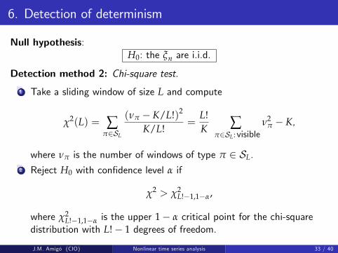
Null hypothesis:H0: the ξn are i.i.d.
Detection method 2: Chi-square test.
1 Take a sliding window of size L and compute
χ2(L) = ∑π2SL
(νπ K/L!)2
K/L!=
L!K ∑
π2SL: visibleν2
π K,
where νπ is the number of windows of type π 2 SL.2 Reject H0 with condence level α if
χ2 > χ2L!1,1α,
where χ2L!1,1α is the upper 1 α critical point for the chi-square
distribution with L! 1 degrees of freedom.
J.M. Amigó (CIO) Nonlinear time series analysis 33 / 40
6. Detection of determinism
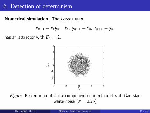
Numerical simulation. The Lorenz map
xn+1 = xnyn zn, yn+1 = xn, zn+1 = yn.
has an attractor with D1 = 2.
4 2 0 2 43
2
1
0
1
2
3
ξn
ξ n+1
Figure. Return map of the x-component contaminated with Gaussianwhite noise (σ = 0.25)
J.M. Amigó (CIO) Nonlinear time series analysis 34 / 40
6. Detection of determinism
0 2000 4000 6000 8000
100
102
104
N
<n(L
,N)>
L=7
L=6L=5
L=4
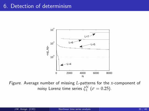
Figure. Average number of missing L-patterns for the x-component ofnoisy Lorenz time series ξN
1 (σ = 0.25).
J.M. Amigó (CIO) Nonlinear time series analysis 35 / 40
6. Detection of determinism
0 2000 4000 6000 8000
100
102
104
N
<n(L
,N)>
b)
L=7
L=6
L=5
Figure. Average number of missing L-patterns for Gaussian white noisewN
1 (σ = 0.25).
J.M. Amigó (CIO) Nonlinear time series analysis 36 / 40
6. Detection of determinism
0 50 100 150 2000
20
40
60
80
100
120
χ2
N(χ
2 )
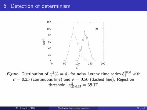
a)
Figure. Distribution of χ2(L = 4) for noisy Lorenz time series ξ10001 with