Page 1
Nonlinear Vibrations of Aerospace Structures
Modeling and Reduction
Time Integration
Periodic Solution
Continuation
Thibaut Detroux | [email protected] 08 October 2018
University of Liège, Belgium
L03 Nonlinear Simulations
Page 2
Why Do We Need High-Fidelity Models?
For better decision-making capability!
Using models, we can access non measurable information
(e.g., stress).
Particular operational conditions (e.g., explosions, earthquakes)
that are difficult/impossible/dangerous to reproduce
experimentally can be simulated. 2
AIRBUS A350XWB Govers et al., ISMA 2014.
Page 3
Why Do We Need High-Fidelity Models?
But also to:
• Reduce dependence on testing (cost and time issues)
• Test design (e.g., sensor and actuator placement)
• Perform virtual prototyping:
A model can predict the behavior of a structure before its
construction.
The parameters of a model can easily be modified to improve the
design (optimization).
3
Page 4
Different Approaches to Model Nonlinear Structures
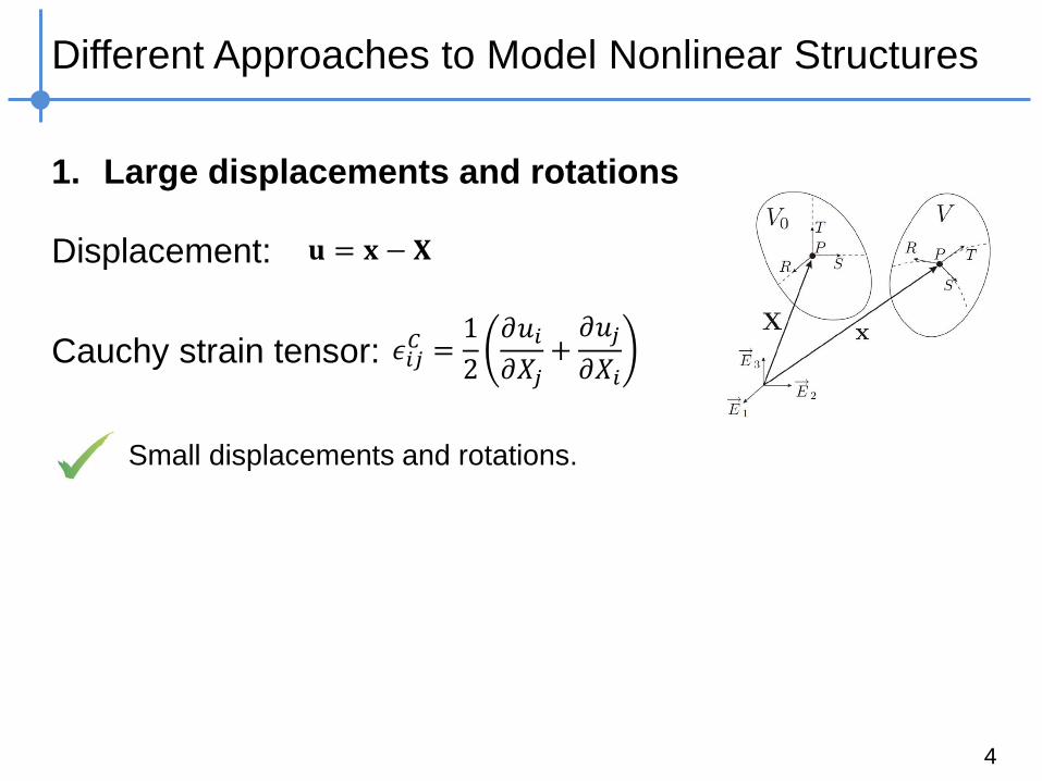
1. Large displacements and rotations
Displacement:
Cauchy strain tensor:
4
𝐮 = 𝐱 − 𝐗
𝜖𝑖𝑗𝐶 =
1
2
𝜕𝑢𝑖𝜕𝑋𝑗
+𝜕𝑢𝑗
𝜕𝑋𝑖
Small displacements and rotations.
Page 5
Different Approaches to Model Nonlinear Structures
1. Large displacements and rotations
Displacement:
Cauchy strain tensor:
5
𝐮 = 𝐱 − 𝐗
𝜖𝑖𝑗𝐶 =
1
2
𝜕𝑢𝑖𝜕𝑋𝑗
+𝜕𝑢𝑗
𝜕𝑋𝑖
Small displacements and rotations.
Not invariant under rigid-body
motion. Cauchy strains cannot be
used if rotation amplitudes are finite.
Prof. O. Brüls, ULiège
Page 6
Different Approaches to Model Nonlinear Structures
1. Large displacements and rotations
Displacement:
Green strain tensor:
6
𝐮 = 𝐱 − 𝐗
𝜖𝑖𝑗𝐺 =
1
2
𝜕𝑢𝑖𝜕𝑋𝑗
+𝜕𝑢𝑗
𝜕𝑋𝑖+
𝜕𝑢𝑘𝜕𝑋𝑖
𝜕𝑢𝑘𝜕𝑋𝑗
3
𝑘=1
Large displacements and rotations.
Nonlinear measure of deformation. Geometrical nonlinearities
can be considered in the elastic force model.
Page 7
Different Approaches to Model Nonlinear Structures
1. Large displacements and rotations
7
Deployable space structure Prof. O. Brüls, ULiège
Landing gear mechanism Prof. O. Brüls, ULiège
Page 8
Different Approaches to Model Nonlinear Structures
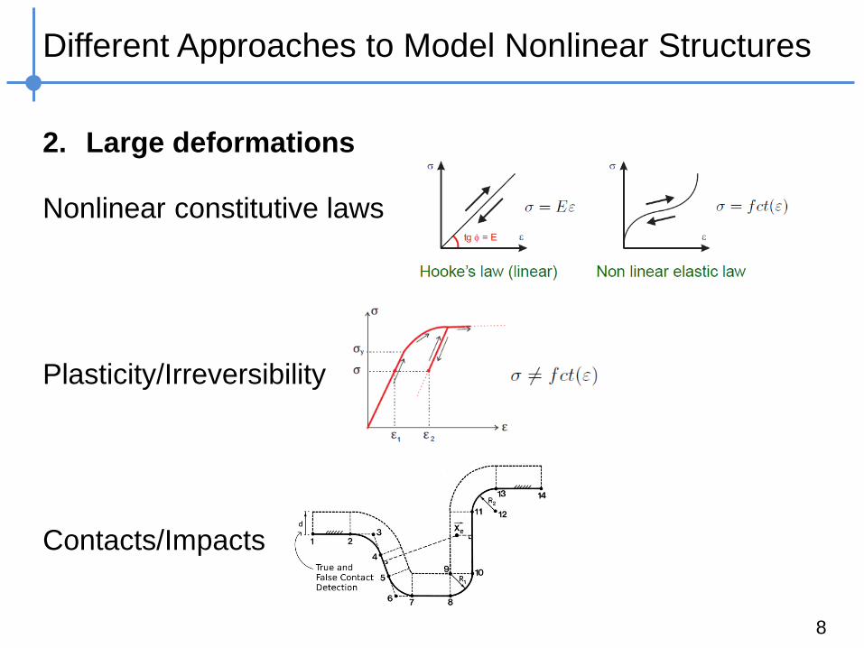
2. Large deformations
Nonlinear constitutive laws
Plasticity/Irreversibility
Contacts/Impacts
8
Page 9
Different Approaches to Model Nonlinear Structures
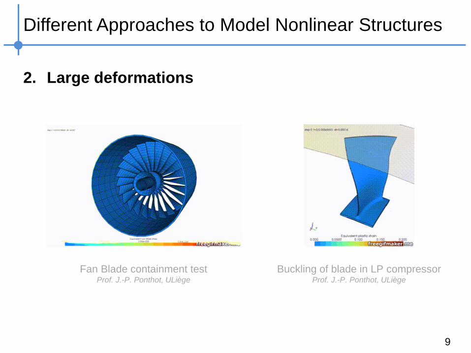
2. Large deformations
9
Buckling of blade in LP compressor Prof. J.-P. Ponthot, ULiège
Fan Blade containment test Prof. J.-P. Ponthot, ULiège
Page 10
Different Approaches to Model Nonlinear Structures
3. Linear structure with localized nonlinearities
10
FOCUS OF THIS COURSE
Page 11
Different Ways to Model Nonlinear Structures
High-fidelity and fast-running modeling
of structures with localized nonlinearities
11
Page 12
Integration of Data-Driven and Computer-Aided Models
What
12
Linear finite element model
Nonlinear
element
Relative displacement
Re
sto
ring
forc
e
Accurate modeling of localized nonlinearities identified
from experimental data (see next lectures).
Page 13
Development of Fast-Running Models
Finite element models may involve thousands (even millions) of
degrees of freedom (DOFs).
For structures with localized nonlinearities, only a few DOFs
are generally involved in nonlinear connections.
Model reduction and substructuring can be applied to
speed up simulations.
13
Page 14
Model Reduction and Substructuring
Reminders from “Mechanical vibrations: Theory and
Applications to Structural Dynamics” (Géradin and Rixen):
Reduction: In most cases, engineers are interested in a smaller
system capturing only lower frequency dynamics. In this case,
a genuine reduction is performed, the reduction method being
seen as a DOF economizer.
Substructuring: In the context of large projects, the analysis is
frequently subdivided into several parts. A separate model is
constructed for each part of the system and reduced (super-
element). The different parts and super-elements are finally
combined to simulate the dynamics of the whole system.
14
Page 15
Model Reduction and Substructuring
Most methods for reducing the size 𝑛 of a system consist in
partitioning the degrees of freedom into 𝑛𝑅 dynamic
retained coordinates (𝑛𝑅 << 𝑛) and 𝑛𝐶 condensed coordinates.
The dynamical behavior of the structure is usually described by
the retained coordinates only.
In this course, the DOFs retained are those connected to
nonlinearities.
15
𝐱 =𝐱𝑅𝐱𝐶
𝐊 =𝐊𝑅𝑅 𝐊𝑅𝐶
𝐊𝐶𝑅 𝐊𝐶𝐶 𝐌 =
𝐌𝑅𝑅 𝐌𝑅𝐶
𝐌𝐶𝑅 𝐌𝐶𝐶
Page 16
Craig-Bampton Method
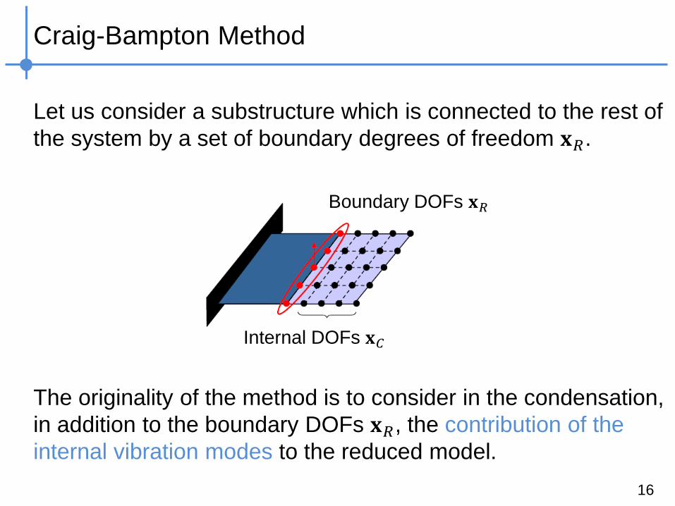
Let us consider a substructure which is connected to the rest of
the system by a set of boundary degrees of freedom 𝐱𝑅.
The originality of the method is to consider in the condensation,
in addition to the boundary DOFs 𝐱𝑅, the contribution of the
internal vibration modes to the reduced model.
16
Boundary DOFs 𝐱𝑅
Internal DOFs 𝐱𝐶
Page 17
Craig-Bampton Method
The dynamical behavior of a substructure is fully described by:
• the static boundary modes resulting from the static
condensation,
• the subsystem eigenmodes in clamped boundary
configuration.
17
Static mode Vibration mode
Page 18
Craig-Bampton Method
Accordingly, it means that the following transformation may be
applied to the initial degrees of freedom:
where the Guyan’s reduction matrix has been complemented
by the set of 𝑛𝐶 internal vibration modes 𝐱 obtained by solving:
18
𝐱 =𝐈 𝟎
−𝐊𝐶𝐶−1𝐊𝐶𝑅 𝚽𝐶
𝐱𝑅𝐲𝐶
𝑛𝑅 boundary DOFs
𝑛𝐶 intensity parameters
of the internal modes
𝐊𝐶𝐶 − 𝜔 2𝐌𝐶𝐶 𝐱 = 𝟎
𝚽𝐶 = 𝐱 (1) … 𝐱 (𝑛𝐶)
Page 19
Craig-Bampton Method
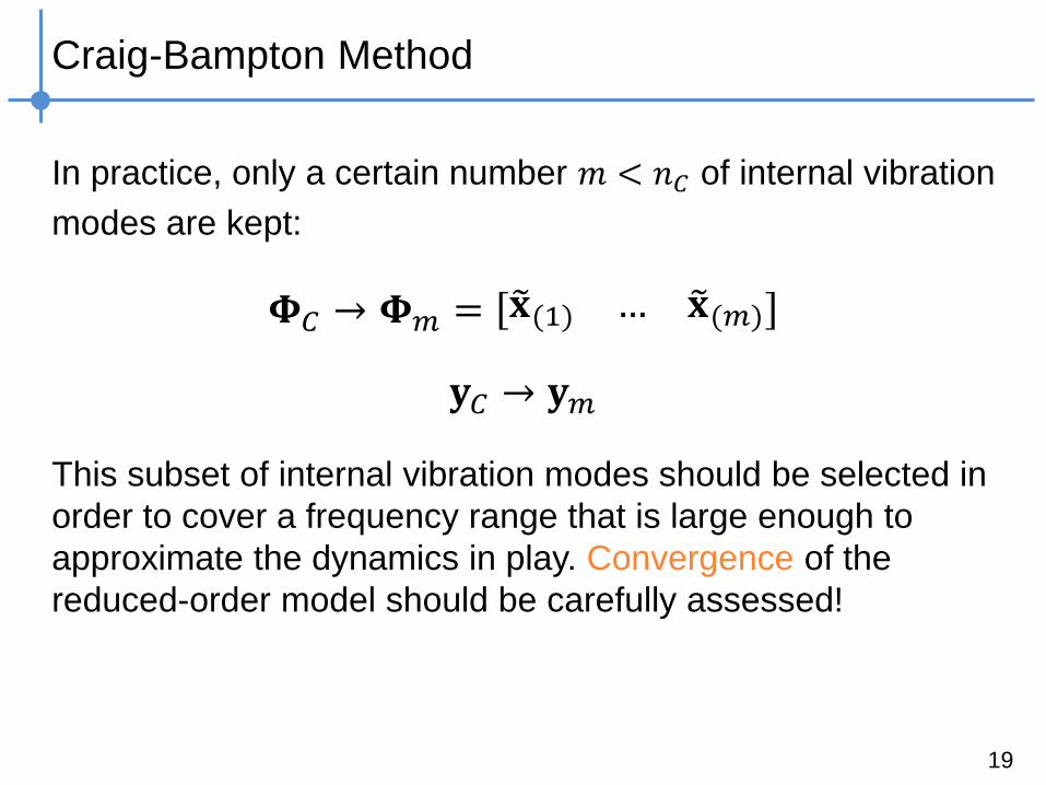
In practice, only a certain number 𝑚 < 𝑛𝐶 of internal vibration
modes are kept:
This subset of internal vibration modes should be selected in
order to cover a frequency range that is large enough to
approximate the dynamics in play. Convergence of the
reduced-order model should be carefully assessed!
19
𝚽𝐶 → 𝚽𝑚 = 𝐱 (1) … 𝐱 (𝑚)
𝐲𝐶 → 𝐲𝑚
Page 20
Craig-Bampton Method
Final reduction matrix of dimension 𝑛 × 𝑛𝑅 +𝑚 :
Reduced stiffness and mass matrices:
Under the assumption of proportional damping, reduced
damping matrix can be defined as
20
𝐑 =𝐈 𝟎
−𝐊𝐶𝐶−1𝐊𝐶𝑅 𝚽𝑚
𝐊 = 𝐑𝑇𝐊𝐑 𝐌 = 𝐑𝑇𝐌𝐑
𝐂 = 𝛼𝐊 + β𝑴
Page 21
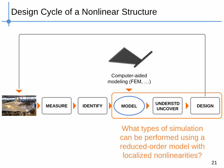
Design Cycle of a Nonlinear Structure
What
21
MEASURE MODEL IDENTIFY UNDERSTD
UNCOVER DESIGN
Computer-aided
modeling (FEM, …)
What types of simulation
can be performed using a
reduced-order model with
localized nonlinearities?
Page 22
Different Ways to Model Nonlinear Structures
Standard Nonlinear Simulations:
Nonlinear Time Integration
22
Page 23
Time Integration Is a Simulation Standard
Simulate the time response of a nonlinear system by solving its
governing equations of motion using numerical algorithms
23
𝐌𝐱 𝑡 + 𝐂𝐱 𝑡 + 𝐊𝐱 𝑡 + 𝐟𝑛𝑙 𝐱, 𝐱 = 𝐟𝑒𝑥𝑡(𝑡)
𝑞1 (m)
Time 𝑡 (s)
𝑞𝑛 (m)
Time 𝑡 (s)
. . .
Page 24
Time Integration Is a Simulation Standard
24
𝐱0 = 𝐱 𝑡0 , 𝐱 0 = 𝐱 𝑡0
Given
𝐌𝐱 𝑛+1 + 𝐂𝐱 𝑛+1 + 𝐊𝐱𝑛+1 + 𝐟𝑛𝑙,𝑛+1 = 𝐟𝑒𝑥𝑡,𝑛+1
Compute 𝐱𝑛+1 = 𝐱 𝑡𝑛+1
Such that
𝐌𝐱 𝑡 + 𝐂𝐱 𝑡 + 𝐊𝐱 𝑡 + 𝐟𝑛𝑙 𝐱, 𝐱 = 𝐟𝑒𝑥𝑡(𝑡)
EOMs:
Initial cond.:
Page 25
Newmark’s Iterative Scheme for Nonlinear Systems
25
Compute 0x
Time incrementation htt nn 1
Prediction
0
5.0
1
1
2
1
1
n
nnnn
nnn
hh
h
x
xxxx
xxx
Residual vector evaluation
1,111 nextnnn ffxMr
Calculation of the correction
00,,,, xxSffM ext
Convergence ?
11 nn fr
),( 000,
1
0 xxffMx
ext
11)( nn rxxS
Correction
xxx
xxx
xxx
211
11
11
1
h
h
nn
nn
nn
Yes
No
(See Géradin and Rixen’s book for more details)
Page 26
Time Step ℎ, 𝛽 and 𝛾 Are Key Parameters
26
Compute 0x
Time incrementation htt nn 1
Prediction
0
5.0
1
1
2
1
1
n
nnnn
nnn
hh
h
x
xxxx
xxx
Residual vector evaluation
1,111 nextnnn ffxMr
Calculation of the correction
00,,,, xxSffM ext
Convergence ?
11 nn fr
),( 000,
1
0 xxffMx
ext
11)( nn rxxS
Correction
xxx
xxx
xxx
211
11
11
1
h
h
nn
nn
nn
Yes
No
(See Géradin and Rixen’s book for more details)
Page 27
27
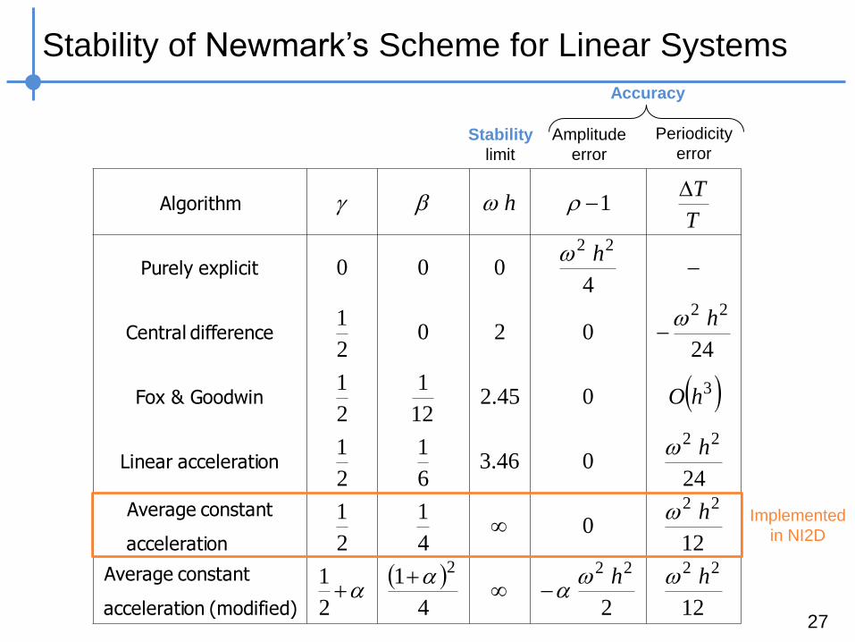
Stability of Newmark’s Scheme for Linear Systems
1224
1
2
1
120
4
1
2
1
24046.3
6
1
2
1
045.212
1
2
1
24020
2
1
4000
1
22222
22
22
3
22
22
hh
h
h
hO
h
h
T
Th
(modified)onaccelerati
constantAverage
onaccelerati
constantAverage
onacceleratiLinear
Goodwin&Fox
differenceCentral
explicitPurely
Algorithm
Amplitude
error
Periodicity
error Stability
limit
Accuracy
Implemented
in NI2D
Page 28
Why Newmark and Not Runge-Kutta (ode45)?
Fixed time step
Convenient for FE models with high eigenfrequencies.
Control on stability and accuracy
Demonstrated for linear systems with 𝛽,𝛾 and time step ℎ.
Possibility to add numerical damping
Use of the 𝛼 parameter, or HHT scheme (more accurate).
Newmark’s scheme is implemented in most commercial FE
software.
28
Page 29
Influence of the Time Step / Sampling Frequency
Rule of thumb: For a periodicity error of 1%, taking higher
harmonics into account, consider at least
29
𝑓𝑠 > 200𝑓
Frequency of interest
in the signal
Sampling frequency = 1/time step
Page 30
Influence of the Time Step / Sampling Frequency
For
30
Page 31
Different Ways to Model Nonlinear Structures
Advanced Nonlinear Simulations:
Nonlinear Frequency Responses and Modes
31
Page 32
Limitations of Time Integration
Time simulations provide useful information about structural
dynamics but they can be time consuming.
32
EXCITATION:
sine, swept-sine, etc. NL SYSTEM
Time
Disp.
Page 33
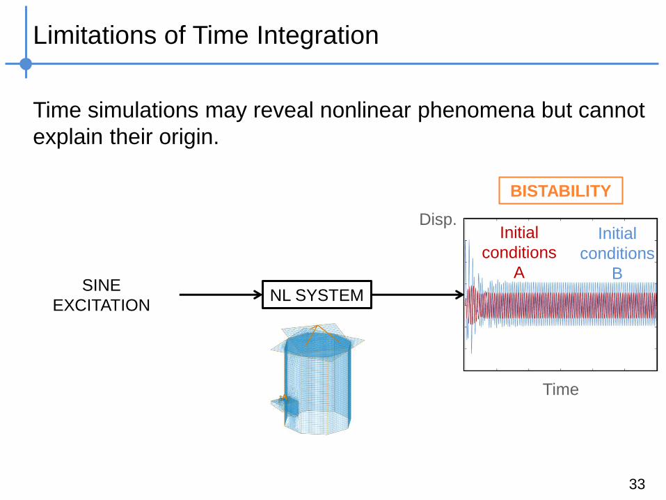
Limitations of Time Integration
Time simulations may reveal nonlinear phenomena but cannot
explain their origin.
33
SINE
EXCITATION NL SYSTEM
Initial
conditions
A
Time
Disp. Initial
conditions
B
BISTABILITY
Page 34
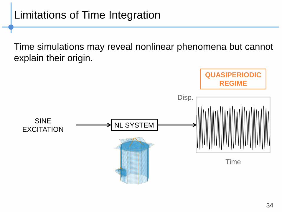
Limitations of Time Integration
Time simulations may reveal nonlinear phenomena but cannot
explain their origin.
34
SINE
EXCITATION NL SYSTEM
Time
Disp.
QUASIPERIODIC
REGIME
Page 35
Limitations of Time Integration
Time simulations may reveal nonlinear phenomena but cannot
explain their origin.
35
SWEPT-SINE
EXCITATION NL SYSTEM
Time / sweep frequency
Disp.
AMPLITUDE
JUMPS
Page 36
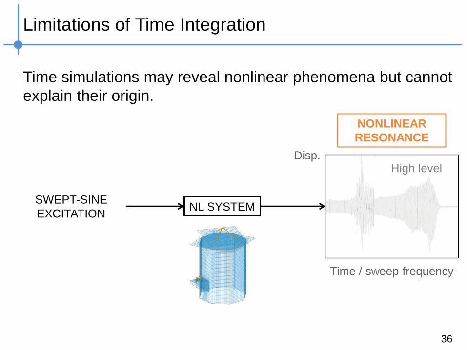
Limitations of Time Integration
Time simulations may reveal nonlinear phenomena but cannot
explain their origin.
36
SWEPT-SINE
EXCITATION NL SYSTEM
Time / sweep frequency
Disp.
NONLINEAR
RESONANCE
5 20 30 70-100
0
100
Low
High level
level
Page 37
Nonlinear normal modes (NNMs) – See Next Lecture
NNMs are obtained by computing branches of periodic
solutions of the underlying undamped and unforced model:
NNMs are useful because:
They describe the deformations at resonance of the
structure.
They describe how modal parameters evolve with
motion amplitude.
37
𝐌𝐱 𝑡 + 𝐊𝐱 𝑡 + 𝐟𝑛𝑙 𝐱 = 0
Page 38
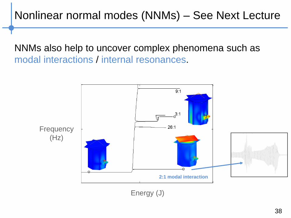
Nonlinear normal modes (NNMs) – See Next Lecture
NNMs also help to uncover complex phenomena such as
modal interactions / internal resonances.
38
Energy (J)
Frequency
(Hz)
5 20 30 70-100
0
100
2:1 modal interaction
Page 39
Nonlinear Frequency Response Curves (NFRCs)
NFRCs are obtained by computing branches of periodic
solutions of the damped model when submitted to a harmonic
excitation:
39
𝐌𝐱 𝑡 + 𝐂𝐱 𝑡 + 𝐊𝐱 𝑡 + 𝐟𝑛𝑙 𝐱, 𝐱 = 𝐟𝑒𝑥𝑡(𝜔, 𝑡)
Time (s)
Displacement
𝑇 =2𝜋
𝜔
Page 40
Nonlinear Frequency Response Curves (NFRCs)
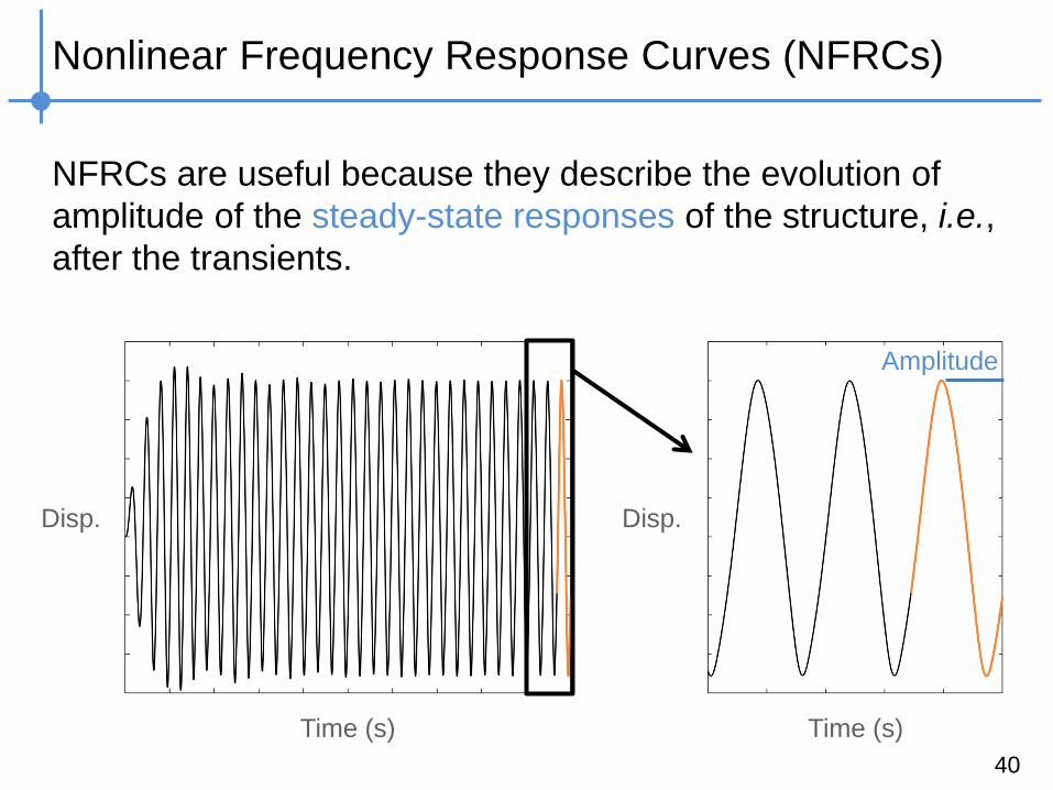
NFRCs are useful because they describe the evolution of
amplitude of the steady-state responses of the structure, i.e.,
after the transients.
40
Time (s)
Disp.
Time (s)
Disp.
Amplitude
Page 41
Nonlinear Frequency Response Curves (NFRCs)
NFRCs are useful because they describe the evolution of
amplitude of the steady-state responses of the structure, i.e.,
after the transients.
41 Frequency 𝜔
Amplitude
Page 42
Nonlinear Frequency Response Curves (NFRCs)
The representative variable is usually chosen as the vibration
amplitude of one of the DOFs, and is represented with respect
to the frequency 𝜔.
42 Frequency 𝜔
Amplitude
of 𝐱𝒊
Page 43
Nonlinear Frequency Response Curves (NFRCs)
NFRCs can be seen as the nonlinear extension of linear
frequency response curves (LFRCs), or FRFs.
43
Amplitude
Frequency 𝜔
NFRC
LFRC
Page 44
Nonlinear Frequency Response Curves (NFRCs)
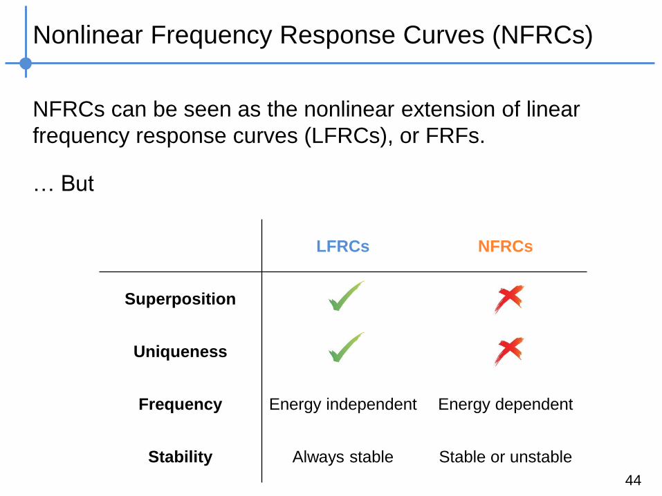
NFRCs can be seen as the nonlinear extension of linear
frequency response curves (LFRCs), or FRFs.
… But
44
LFRCs NFRCs
Superposition
Uniqueness
Frequency Energy independent Energy dependent
Stability Always stable Stable or unstable
Page 45
Nonlinear Frequency Response Curves (NFRCs)
The
45
Page 46
Nonlinear Frequency Response Curves (NFRCs)
NNMs also help to uncover complex phenomena such as
amplitude jumps.
46
Frequency 𝜔
Amplitude
Page 47
Nonlinear Frequency Response Curves (NFRCs)
NNMs also help to uncover complex phenomena such as
quasiperiodic regime.
47
Frequency 𝜔
Amplitude
Page 48
Nonlinear Frequency Response Curves (NFRCs)
NNMs also help to uncover complex phenomena such as
bistability.
48
Frequency 𝜔
Amplitude
Page 49
Towards the Continuation of NNMs and NFRCs
Trivia
49
1. Computation of Periodic Solutions
Time (s)
Displacement
TOPIC OF THIS LECTURE
Page 50
Towards the Continuation of NNMs and NFRCs
Trivia
50
2. Continuation procedure
Frequency 𝜔
Amplitude
TOPIC OF THIS LECTURE
Page 51
Towards the Continuation of NNMs and NFRCs
Trivia
51
3. Stability analysis
Unstable
Stable
Frequency 𝜔
Amplitude
SEE NEXT LECTURES
Page 52
Towards the Continuation of NNMs and NFRCs
Trivia
52
4. Bifurcation analysis
Fold Neimark-Sacker
Frequency 𝜔
Amplitude
SEE NEXT LECTURES
Page 53
Different Ways to Model Nonlinear Structures
Computation of Periodic Solutions
53
Page 54
Mathematical Representation of a Periodic Solution
There are at least 3 approaches to describe a periodic solution.
54
Displacement
(m)
Time (s)
𝑇
Page 55
Mathematical Representation of a Periodic Solution
There are at least 3 approaches to describe a periodic solution.
Initial conditions 𝐱0 𝐱 0𝑇 and the period 𝑇.
55
= + Time integration
over 𝑇
Page 56
Mathematical Representation of a Periodic Solution
There are at least 3 approaches to describe a periodic solution.
Piecewise polynomial functions and the period 𝑇.
56
= + +
Page 57
Mathematical Representation of a Periodic Solution
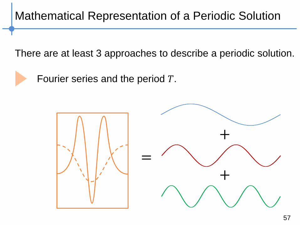
There are at least 3 approaches to describe a periodic solution.
Fourier series and the period 𝑇.
57
=
+
+
Page 58
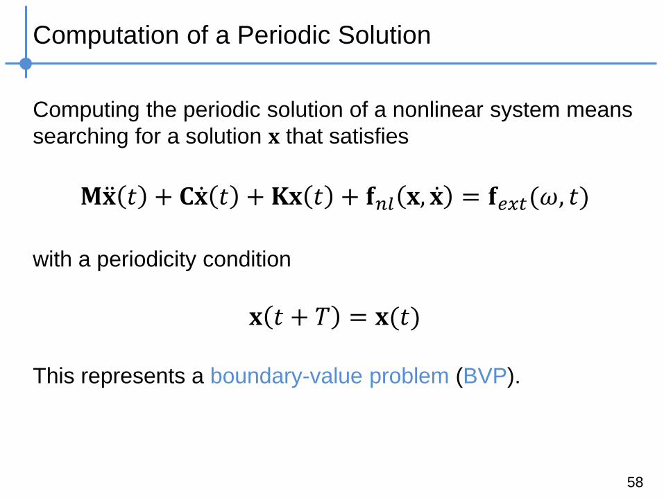
Computation of a Periodic Solution
Computing the periodic solution of a nonlinear system means
searching for a solution 𝐱 that satisfies
with a periodicity condition
This represents a boundary-value problem (BVP).
58
𝐌𝐱 𝑡 + 𝐂𝐱 𝑡 + 𝐊𝐱 𝑡 + 𝐟𝑛𝑙 𝐱, 𝐱 = 𝐟𝑒𝑥𝑡(𝜔, 𝑡)
𝐱 𝑡 + 𝑇 = 𝐱(𝑡)
Page 59
Computation of a Periodic Solution
There are three approaches to solve this BVP.
Based on initial conditions 𝐱0 𝐱 0𝑇.
Shooting technique
Based on piecewise polynomial functions.
Orthogonal collocation (not discussed here)
Based on Fourier series.
Harmonic balance method
59
Page 60
Shooting Technique
Optimization of the initial state of a system 𝐱0 𝐱 0𝑇 to obtain a
periodic solution after time integration over a period 𝑇.
60
𝑇
« Angle » = 𝐱0
« Power » = 𝐱 0
Page 61
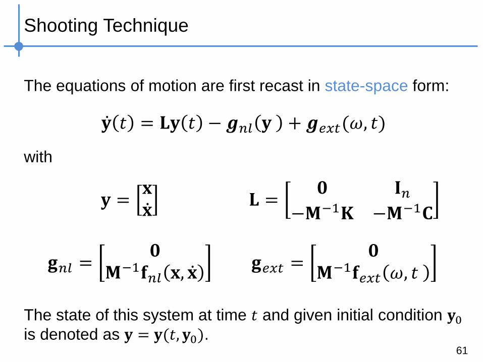
Shooting Technique
The equations of motion are first recast in state-space form:
with
The state of this system at time 𝑡 and given initial condition 𝐲0
is denoted as 𝐲 = 𝐲(𝑡, 𝐲0).
61
𝐲 𝑡 = 𝐋𝐲 𝑡 − 𝒈𝑛𝑙 𝐲 + 𝒈𝑒𝑥𝑡(𝜔, 𝑡)
𝐲 =𝐱𝐱
𝐋 =𝟎 𝐈𝑛
−𝐌−1𝐊 −𝐌−1𝐂
𝐠𝑒𝑥𝑡 =𝟎
𝐌−1𝐟𝑒𝑥𝑡 𝜔, 𝑡 𝐠𝑛𝑙 =
𝟎𝐌−1𝐟𝑛𝑙 𝐱, 𝐱
Page 62
Shooting Technique
An initial state 𝐲0,𝑝 leads to a periodic solution if
where 𝐲 𝑇, 𝐲0,𝑝 is computed from time integration of the EOMs.
The shooting technique consists in computing 𝐲0,𝑝 that satisfies
𝐡𝑠ℎ𝑜𝑜𝑡𝑖𝑛𝑔 = 𝟎 for 𝑇 known a priori (NFRC) or not (NNM).
In the case of a harmonic excitation with frequency 𝜔, 𝑇 can be
approximated as 𝑇 = 2𝜋/𝜔.
62
𝐡𝑠ℎ𝑜𝑜𝑡𝑖𝑛𝑔 ≡ 𝐲 𝑇, 𝐲0,𝑝 − 𝐲0,𝑝 = 𝟎
Page 63
Shooting Technique Scheme (for NFRCs)
63
Initial state
at iteration 𝑖
𝐲0,𝑝𝑖
Evaluation of
𝐡𝑠ℎ𝑜𝑜𝑡𝑖𝑛𝑔
= 𝐲 𝑇, 𝐲0,𝑝𝑖 − 𝐲0,𝑝
𝑖
Initial guess for
initial state
𝐲0,𝑝0
< 𝜖?
𝑇
NO: Correction (e.g., Newton-Raphson)
Time integration YES
END
Page 64
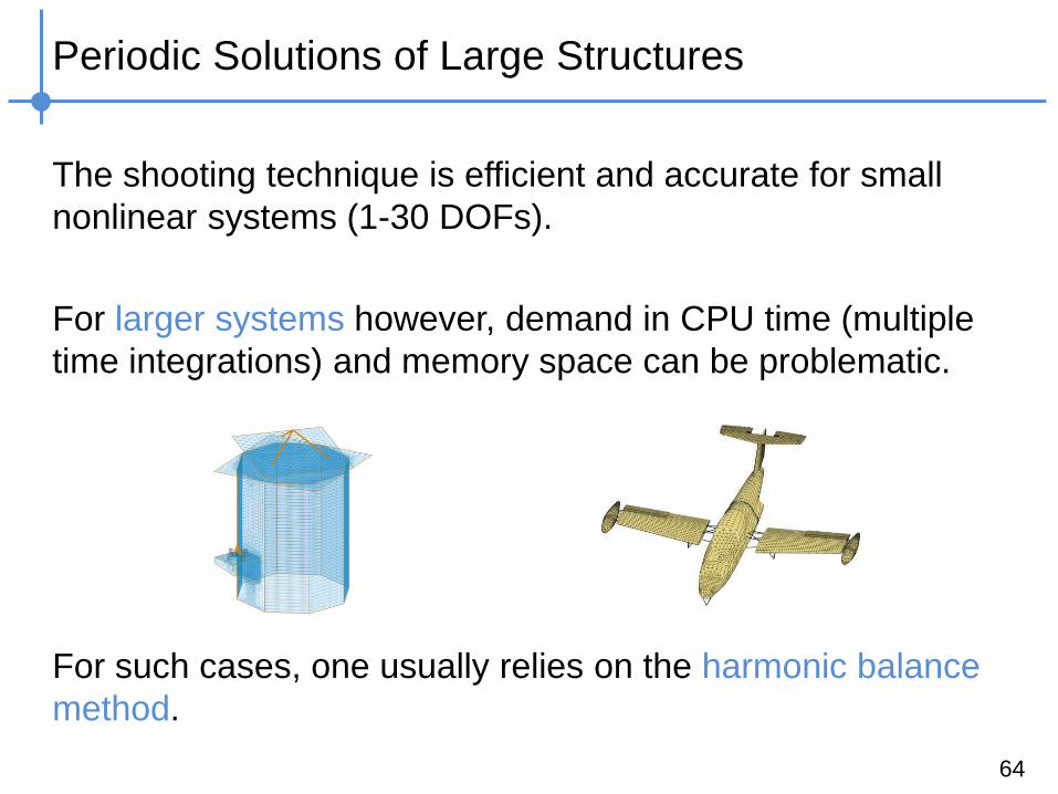
Periodic Solutions of Large Structures
The shooting technique is efficient and accurate for small
nonlinear systems (1-30 DOFs).
For larger systems however, demand in CPU time (multiple
time integrations) and memory space can be problematic.
For such cases, one usually relies on the harmonic balance
method.
64
Page 65
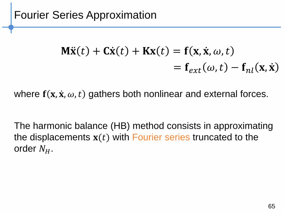
Fourier Series Approximation
where 𝐟 𝐱, 𝐱 , 𝜔, 𝑡 gathers both nonlinear and external forces.
The harmonic balance (HB) method consists in approximating
the displacements 𝐱(𝑡) with Fourier series truncated to the
order 𝑁𝐻.
65
𝐌𝐱 𝑡 + 𝐂𝐱 𝑡 + 𝐊𝐱 𝑡 = 𝐟 𝐱, 𝐱 , 𝜔, 𝑡
= 𝐟𝑒𝑥𝑡 𝜔, 𝑡 − 𝐟𝑛𝑙 𝐱, 𝐱
Page 66
Fourier Series Approximation
The new unknowns are the Fourier coefficients 𝐳, with
66
𝐳 = 𝐜0𝐱𝑇 𝒔1
𝐱𝑇 𝐜1𝐱𝑇 … 𝒔𝑁𝐻
𝐱 𝑇 𝐜𝑁𝐻
𝐱 𝑇 𝑇
𝐌𝐱 𝑡 + 𝐂𝐱 𝑡 + 𝐊𝐱 𝑡 = 𝐟 𝐱, 𝐱 , 𝜔, 𝑡
𝑛𝑍 = 𝑛(2𝑁𝐻 + 1) unknowns
𝐱 𝑡 =𝐜0𝐱
2+ 𝐬𝑘
𝐱 sin 𝑘𝜔𝑡 + 𝐜𝑘𝐱 cos(𝑘𝜔𝑡)
𝑁𝐻
𝑘=1
Page 67
Fourier Series Approximation
The Fourier coefficients of 𝐟 are denoted by 𝐛, with
67
𝐟 𝐱, 𝐱 , 𝜔, 𝑡 =𝐜0𝐟
2+ 𝐬𝑘
𝐟 sin 𝑘𝜔𝑡 + 𝐜𝑘𝐟 cos(𝑘𝜔𝑡)
𝑁𝐻
𝑘=1
𝐌𝐱 𝑡 + 𝐂𝐱 𝑡 + 𝐊𝐱 𝑡 = 𝐟 𝐱, 𝐱 , 𝜔, 𝑡
𝐛 = 𝐜0𝐟𝑇 𝒔1
𝐟 𝑇 𝐜1𝐟𝑇 … 𝒔𝑁𝐻
𝐟 𝑇 𝐜𝑁𝐻
𝐟 𝑇 𝑇
= 𝐛(𝐳) since 𝐟 depends on 𝐱.
Page 68
Fourier Series Approximation
Displacements and forces can be recast into a more compact
form
where ⊗ denotes the Kronecker tensor product, 𝐈𝑛 represents
the identity matrix and where 𝐐(𝑡) is the orthogonal
trigonometric basis:
68
𝐱 𝑡 = 𝐐 𝑡 ⊗ 𝐈𝑛 𝐳
𝐟 𝑡 = 𝐐 𝑡 ⊗ 𝐈𝑛 𝐛
𝐐 𝑡 =1
2 sin 𝜔𝑡 cos 𝜔𝑡 … sin 𝑁𝐻𝜔𝑡 cos 𝑁𝐻𝜔𝑡
Page 69
Fourier Series Approximation
With this formulation, velocities can also be defined using
Fourier series:
where
69
𝐱 𝑡 = 𝐐 𝑡 ⊗ 𝐈𝑛 𝐳 = 𝐐 𝑡 𝛁 ⊗ 𝐈𝑛 𝐳
𝛁 =
0
⋱
𝛁𝑘
⋱
𝛁𝑁𝐻
𝛁𝑘 =0 −𝑘𝜔𝑘𝜔 0
Page 70
Fourier Series Approximation
With this formulation, accelerations can also be defined using
Fourier series:
where
70
𝛁𝟐 = 𝛁𝛁 =
0
⋱
𝛁𝑘2
⋱
𝛁𝑁𝐻
2
𝛁𝑘2 =
− 𝑘𝜔 2 0
0 − 𝑘𝜔 2
𝐱 𝑡 = 𝐐 𝑡 ⊗ 𝐈𝑛 𝐳 = 𝐐 𝑡 𝛁2 ⊗ 𝐈𝑛 𝐳
Page 71
Equations of Motion in the Frequency Domain
As
71
𝐌 𝐐 𝑡 𝛁2 ⊗ 𝐈𝑛 𝐳 + 𝐂 𝐐 𝑡 𝛁 ⊗ 𝐈𝑛 𝐳
+𝐊 𝐐 𝑡 ⊗ 𝐈𝑛 𝐳 = 𝐐 𝑡 ⊗ 𝐈𝑛 𝐛
𝐌𝐱 𝑡 + 𝐂𝐱 𝑡 + 𝐊𝐱 𝑡 = 𝐟 𝐱, 𝐱 , 𝜔, 𝑡
Fourier series
approximation
This expression can be further simplified using:
- Galerkin procedure (to remove time dependency).
- Kronecker product properties.
Page 72
Equations of Motion in the Frequency Domain
In a more compact form:
where 𝐀 describes the linear dynamics
72
𝐀 = 𝛁2 ⊗𝐌+ 𝛁⊗ 𝐂 + 𝐈2𝑁𝐻+1 ⊗𝐊
𝐊
𝐊 − 𝜔2𝐌 −𝜔𝐂
𝜔𝐂 𝐊 − 𝜔2𝐌
⋱
𝐊 − 𝑁𝐻𝜔2𝐌 −𝑁𝐻𝜔𝐂
𝑁𝐻𝜔𝐂 𝐊 − 𝑁𝐻𝜔2𝐌
=
𝐡 𝐳, 𝜔 ≡ 𝐀 𝜔 𝐳 − 𝐛 𝐳 = 𝟎
Page 73
Equations of Motion in the Frequency Domain
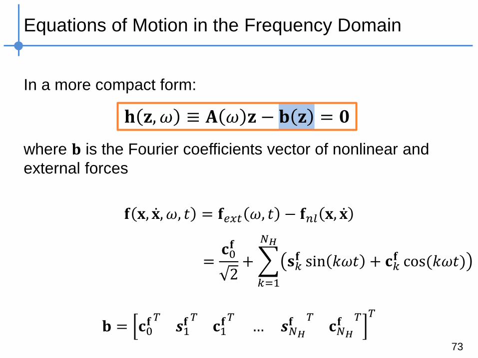
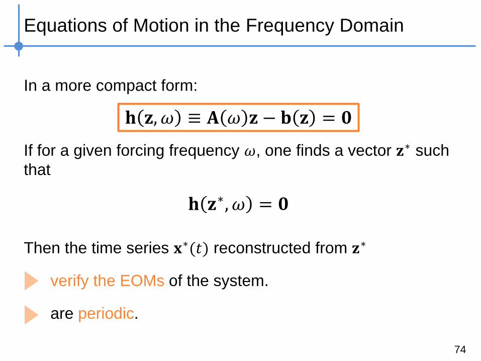
In a more compact form:
where 𝐛 is the Fourier coefficients vector of nonlinear and
external forces
73
=𝐜0𝐟
2+ 𝐬𝑘
𝐟 sin 𝑘𝜔𝑡 + 𝐜𝑘𝐟 cos(𝑘𝜔𝑡)
𝑁𝐻
𝑘=1
𝐛 = 𝐜0𝐟𝑇 𝒔1
𝐟 𝑇 𝐜1𝐟𝑇 … 𝒔𝑁𝐻
𝐟 𝑇 𝐜𝑁𝐻
𝐟 𝑇 𝑇
𝐟 𝐱, 𝐱 , 𝜔, 𝑡 = 𝐟𝑒𝑥𝑡 𝜔, 𝑡 − 𝐟𝑛𝑙 𝐱, 𝐱
𝐡 𝐳, 𝜔 ≡ 𝐀 𝜔 𝐳 − 𝐛 𝐳 = 𝟎
Page 74
Equations of Motion in the Frequency Domain
In a more compact form:
If for a given forcing frequency 𝜔, one finds a vector 𝐳∗ such
that
Then the time series 𝐱∗(𝑡) reconstructed from 𝐳∗
verify the EOMs of the system.
are periodic.
74
𝐡 𝐳, 𝜔 ≡ 𝐀 𝜔 𝐳 − 𝐛 𝐳 = 𝟎
𝐡 𝐳∗, 𝜔 = 𝟎
Page 75
Equations of Motion in the Frequency Domain
𝐡 𝐳,𝜔 = 0 is a nonlinear algebraic equation (easier to
solve than time integrations as in shooting technique).
𝐳 are the Fourier coefficients of the displacements and the
new unknowns of the problem (usually less than for
orthogonal collocation).
For NFRCs, 𝜔 is the forcing frequency and is a system
parameter.
75
𝐡 𝐳, 𝜔 ≡ 𝐀 𝜔 𝐳 − 𝐛 𝐳 = 𝟎
Page 76
Harmonic Balance Parameters
76
Number of harmonics 𝑁𝐻
retained in the Fourier series.
Page 77
Harmonic Balance Parameters
77
Number of time samples 𝑁 in the
Fourier transform.
Page 78
Harmonic Balance Parameters
78
Stability parameters (see next
lectures)
Page 79
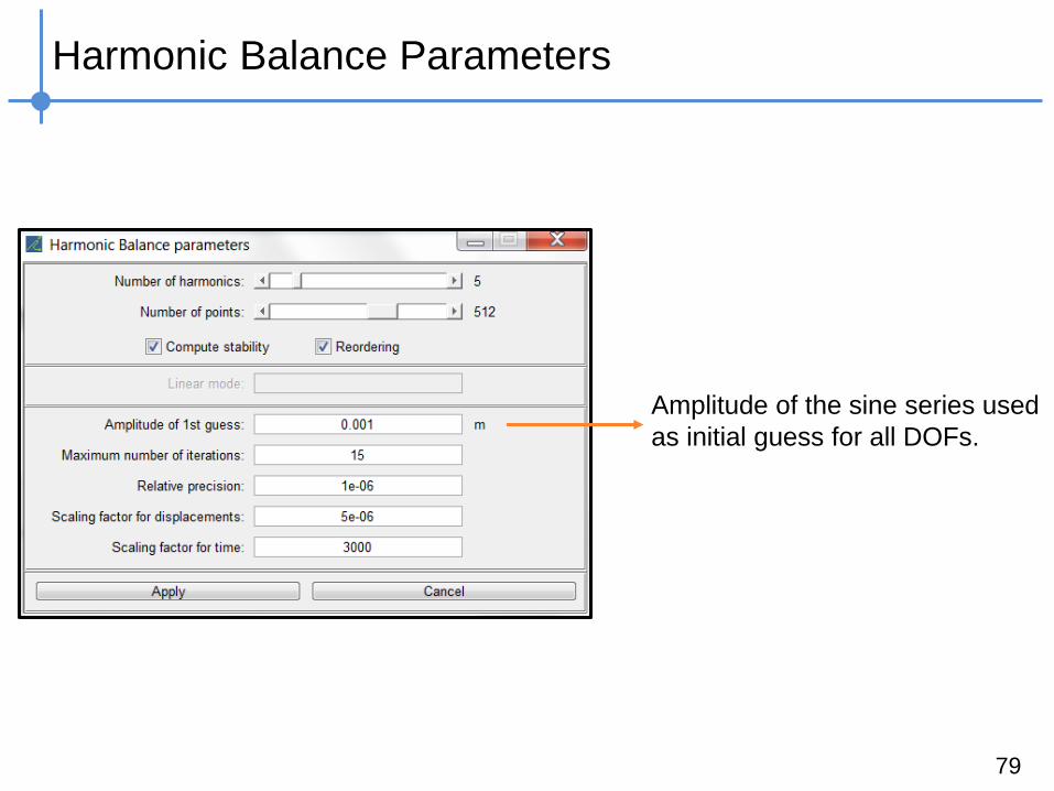
Harmonic Balance Parameters
79
Amplitude of the sine series used
as initial guess for all DOFs.
Page 80
Harmonic Balance Parameters
80
The Newton-Raphson procedure
fails if this number of iterations is
exceeded.
Page 81
Harmonic Balance Parameters
81
The Newton-Raphson procedure
stops if the relative error is
smaller than this precision.
Page 82
Harmonic Balance Parameters
82
Because the frequency (e.g.,
30Hz = 188rad/s) and the
amplitude (e.g., 0.001m) have
different orders of magnitude,
time and displacements have to
be rescaled to avoid ill
conditioning.
Page 83
Harmonic Balance Method: In Summary
Adaptations of the method improve its performance (alternating
time-frequency method, chain rule, …) – not discussed here.
83
Efficient
Harmonic coefficients
available
Less accurate
Many harmonics are
sometimes required
PROS CONS
Filtering
Page 84
Computation of Periodic Solutions: In Summary
Periodic solutions of nonlinear structures can be computed with
time-domain (shooting, orthogonal collocation) or frequency-
domain method (harmonic balance).
The differences between these methods lie in their accuracy
and execution time.
Without adaptation, however, the harmonic balance:
- Fails at computing periodic reponses in severe nonlinear
regimes (need for continuation procedure).
- Does not indicate if the solutions can be observed
experimentally or not (need for a stability analysis).
84
Page 85
Different Ways to Model Nonlinear Structures
Computation of Branches
of Periodic Solutions
85
Page 86
Computation of Branches of Periodic Solutions
86
Numerical methods to go from
single periodic solutions…
y
Frequency
… to a
branch of periodic solutions
y
Frequency
Page 87
Mathematical Definition of a Branch of Periodic Solutions
Let us consider a function 𝑭:𝑹𝑛+1 → 𝑹𝑛. A branch is a set of
solutions 𝑭 𝒙, 𝜆 = 𝟎, where 𝒙 are the state variables and 𝜆 is a
system parameter.
The branch can be represented in a 2D plane through the
evolution of a representative variable 𝑦 = 𝑦(𝒙) w.r.t. 𝜆. 87
y
Parameter 𝜆
𝐹 = 0
Page 88
Types of Branch
In this course, the branch is composed by solutions of the
harmonic balance equation for a nonlinear system:
Nonlinear Frequency Response Curves
Forced and damped system
Nonlinear Normal Modes
Unforced and undamped system 88
𝐡 𝐳, 𝜔 : 𝐑𝑛𝑧+1 → 𝑹𝑛𝑧
Fourier coefficients (= state variables)
Frequency (= system parameter)
Page 89
Sequential Continuation – A Straightforward Approach
Increase the period and use the previously computed periodic
solution as an initial guess for the next computation.
89
Amplitude
𝜔
Previous solution as prediction
𝛥𝜔
Optimization with fixed frequency
Solutions of the branch
Page 90
Sequential Continuation – Scheme
If HB method is already implemented, sequential continuation is
programmed in a few lines.
90
Initial solution
𝐳𝑖 = 𝐳0
Next frequency
𝜔𝑖 = 𝜔𝑖−1 + 𝛥𝜔
New iteration
𝐳𝑖
Convergence
𝐡(𝐳𝑖 , 𝜔𝑖) = 𝟎?
Yes
𝐳𝑖 = 𝐳𝑖−1
No
Correction
(Newton-Raphson,
fminunc, etc.)
Page 91
Sequential Continuation Fails at Turning Points
0.02
1
0.1 𝑠𝑖𝑛(𝜔𝑡)
1
1
Amplitude
Frequency 𝜔
Reference
𝛥𝜔 < 0 𝛥𝜔 > 0
91
Page 92
A New Continuation Scheme
In order to pass through turning points, both the state 𝐳 and the
parameter 𝜔 should vary. This is done through a 2-step
procedure:
92
Amplitude
Frequency 𝜔
Prediction 1
Page 93
A New Continuation Scheme
In order to pass through turning points, both the state 𝐳 and the
parameter 𝜔 should vary. This is done through a 2-step
procedure:
93
Amplitude
Frequency 𝜔
Prediction 1
Corrections 2
Page 94
Predictor Step
Different predictors can be considered:
where 𝐗 = 𝐳 𝜔 𝑇 denotes the unknown vector.
Secant predictor
94
𝐗𝑝𝑟𝑒𝑑𝑖 = 𝐗𝑖−1 + 𝑠𝑖𝐭𝑖
Amp.
Frequency 𝜔
𝑠𝑖
Stepsize
𝐭𝑖
Unit vector
𝐭𝑖 =𝐗𝑖−1 − 𝐗𝑖−2
𝐗𝑖−1 − 𝐗𝑖−2
Page 95
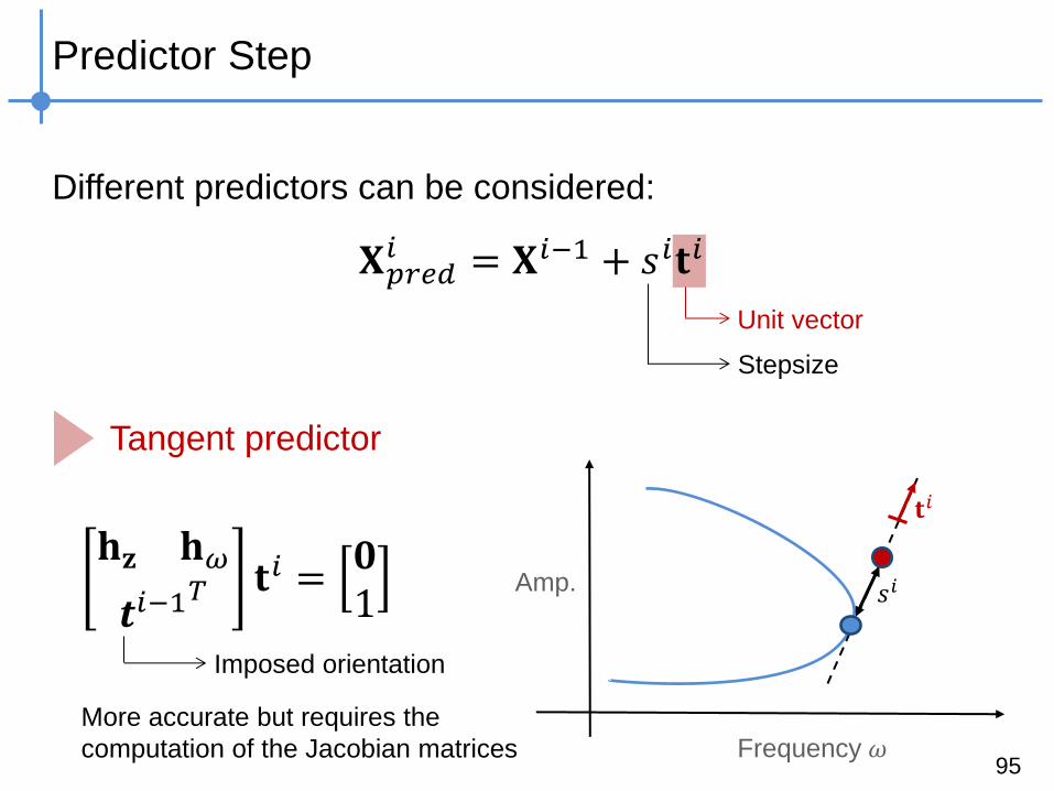
Predictor Step
Different predictors can be considered:
Tangent predictor
95
Amp.
Frequency 𝜔
𝑠𝑖
𝐡𝐳 𝐡𝜔
𝒕𝑖−1𝑇 𝐭𝑖 =
𝟎1
𝐭𝑖
More accurate but requires the
computation of the Jacobian matrices
Imposed orientation
𝐗𝑝𝑟𝑒𝑑𝑖 = 𝐗𝑖−1 + 𝑠𝑖𝐭𝑖
Stepsize
Unit vector
Page 96
Corrector Step
We are looking for a solution of 𝐡 𝐳,𝜔 = 𝟎, with
Two possibilities:
Fix the parameter 𝜔 and only optimize 𝑧.
Cf. sequential continuation
Add another equation to the system.
Pseudo-arclength and Moore-Penrose schemes
96
𝐡 𝐳, 𝜔 : 𝐑𝑛𝑧+1 → 𝑹𝑛𝑧
Page 97
Pseudo-arclength Corrector Step
With the pseudo-arclength scheme, a solution is sought in the
perpendicular direction w.r.t. the prediction.
97
Amp.
Frequency 𝜔
Page 98
Pseudo-arclength Corrector Step
With the pseudo-arclength scheme, a solution is sought in the
perpendicular direction w.r.t. the prediction.
with
98
𝒛 𝑗+1𝑖 = 𝒛 𝑗
𝑖 + 𝚫𝐳 𝑗
𝜔 𝑗+1𝑖 = 𝜔 𝑗
𝑖 + Δ𝜔 𝑗
𝐡𝐳 𝐳 𝑗𝑖 , 𝜔 𝑗 𝐡𝜔 𝐳 𝑗
𝑖 , 𝜔 𝑗
𝐭𝐳𝑖 t𝜔
𝑖
𝚫𝐳 𝐣
𝛥𝜔 𝑗=
−𝐡 𝐳 𝑗𝑖 , 𝜔 𝑗
0
𝑖 = continuation iteration
(𝑗) = corrector iteration
Orthogonality condition
Taylor series expansion
Page 99
Other Correctors
Other corrector definitions can also be used.
With the Moore-Penrose scheme for instance, the correction
direction is updated at each corrector step.
99
Amp.
Frequency 𝜔
Page 100
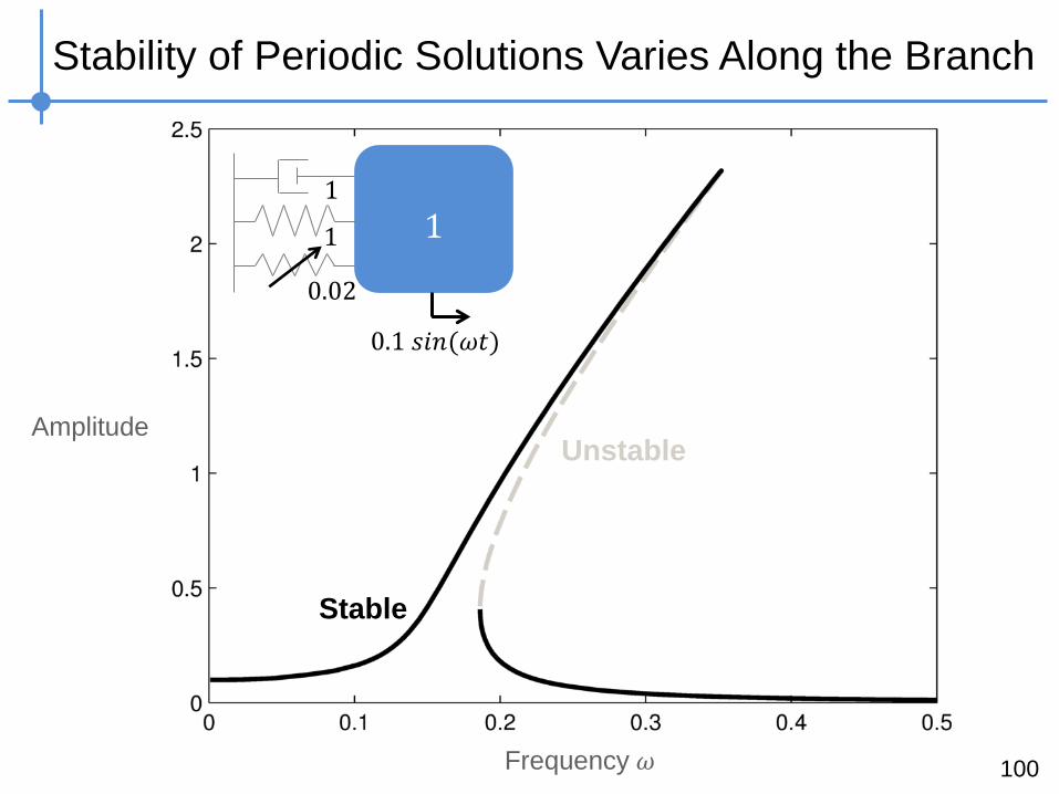
Stability of Periodic Solutions Varies Along the Branch
100
0.02
1
0.1 𝑠𝑖𝑛(𝜔𝑡)
1
1
Amplitude
Frequency 𝜔
Stable
Unstable
Page 101
Periodic Solutions Can be Stable or Unstable
101
Amplitude
Frequency 𝜔
Floquet exponents
(see next lectures)
Page 102
Periodic Solutions Can be Stable or Unstable
102
Amplitude
Frequency 𝜔
Floquet exponents
(see next lectures)
Page 103
Periodic Solutions Can be Stable or Unstable
103
Amplitude
Frequency 𝜔
Floquet exponents
(see next lectures)
Page 104
Periodic Solutions Can be Stable or Unstable
104
Amplitude
Frequency 𝜔
Floquet exponents
(see next lectures)
Page 105
Periodic Solutions Can be Stable or Unstable
105
Amplitude
Frequency 𝜔
Floquet exponents
(see next lectures)
Page 106
Periodic Solutions Can be Stable or Unstable
106
Amplitude
Frequency 𝜔
Floquet exponents
(see next lectures)
Page 107
Periodic Solutions Can be Stable or Unstable
107
Amplitude
Frequency 𝜔
Floquet exponents
(see next lectures)
Page 108
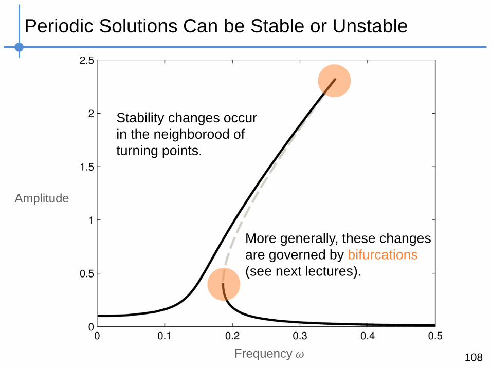
Periodic Solutions Can be Stable or Unstable
108
Amplitude
Frequency 𝜔
More generally, these changes
are governed by bifurcations
(see next lectures).
Stability changes occur
in the neighborood of
turning points.
Page 109
Influence of the Stepsize
Stepsize is a key parameter for the continuation procedure.
109
𝑿𝑝𝑟𝑒𝑑𝑖 = 𝑿𝑖−1 + 𝑠𝑖𝐭𝑖
Amp.
Frequency 𝜔
𝑠𝑖
Stepsize
𝐭𝑖
Unit vector
Page 110
Small Stepsize
Small number of corrections
Good resolution for the branch
Slow continuation procedure
110
Amplitude
Frequency 𝜔
Page 111
Large Stepsize
Fast continuation procedure
Large number of corrections
Poor resolution for the branch
111
Amplitude
Frequency 𝜔
Page 112
Stepsize Strategy
Fixed stepsize
Adaptative stepsize
where 𝑀 is the iteration number for the current correction,
and 𝑀∗ is the optimal iteration number.
112
𝑠𝑖 = constant
𝑠𝑖 =𝑀∗
𝑀𝑠𝑖−1
Page 113
Influence of Harmonic Balance Parameters
With the harmonic balance method, the displacements are
approximated with Fourier series.
Fourier coefficients 𝐳 are computed with the discrete Fourier
transform:
113
𝐱 𝑡 = 𝐜0𝐱 + 𝐬𝑘
𝐱 sin 𝑘𝜔𝑡 + 𝐜𝑘𝐱 cos(𝑘𝜔𝑡)
𝑁𝐻
𝑘=1
𝐳
𝐳 = 𝚪+(𝑁)𝐱
Number of harmonics
Number of time samples (power of 2)
Page 114
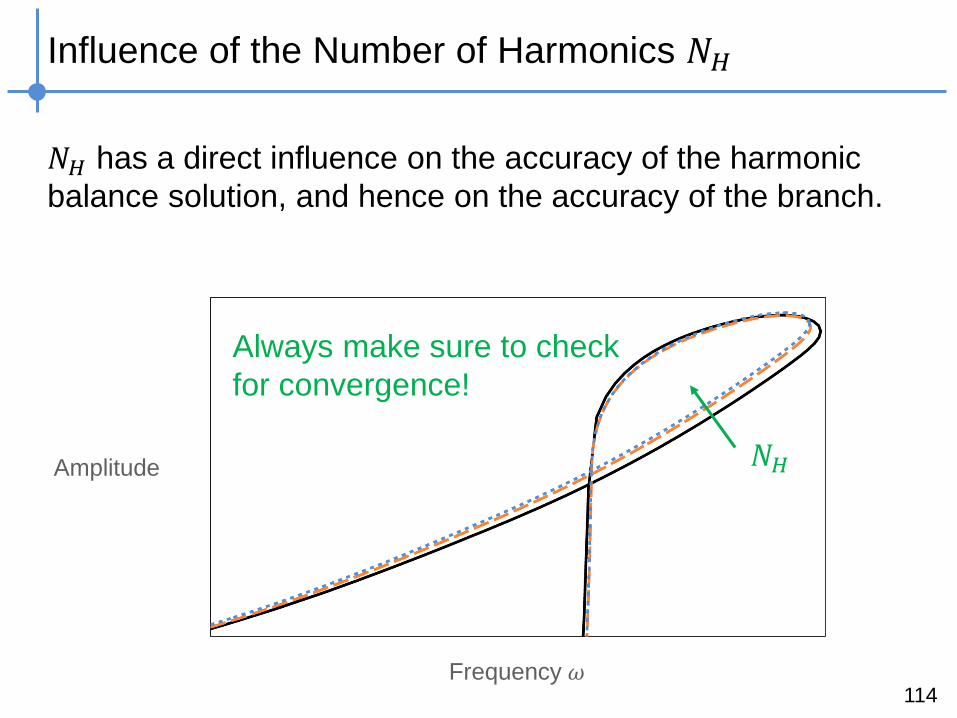
Influence of the Number of Harmonics 𝑁𝐻
𝑁𝐻 has a direct influence on the accuracy of the harmonic
balance solution, and hence on the accuracy of the branch.
114
Amplitude
Frequency 𝜔
𝑁𝐻
Always make sure to check
for convergence!
Page 115
Influence of the Number of Time Samples 𝑁
𝑁 has a direct influence on the discrete Fourier transform, and
the accuracy of the alternating frequency/time-domain method.
115
Amplitude
Frequency 𝜔
Page 116
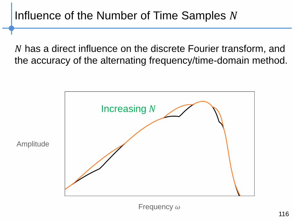
Influence of the Number of Time Samples 𝑁
𝑁 has a direct influence on the discrete Fourier transform, and
the accuracy of the alternating frequency/time-domain method.
116
Increasing 𝑁
Amplitude
Frequency 𝜔
Page 117
Influence of the Number of Time Samples 𝑁
𝑁 has a direct influence on the discrete Fourier transform, and
the accuracy of the alternating frequency/time-domain method.
117
Increasing 𝑁
Amplitude
Frequency 𝜔
Page 118
Influence of the Number of Time Samples 𝑁
𝑁 has a direct influence on the discrete Fourier transform, and
the accuracy of the alternating frequency/time-domain method.
118
Increasing 𝑁
Amplitude
Frequency 𝜔
Always make sure to check
for convergence!
Page 119
Continuation: In Summary
Sequential continuation can be easily implemented to represent
the evolution of the periodic solutions w.r.t. to the frequency 𝜔
but it fails at turning points.
Continuation schemes based on predictor/corrector steps give
the evolution of the periodic solutions in both stable and
unstable regions.
HB and continuation parameters have to be carefully selected
to ensure accuracy and good resolution of the branches.
119


![Nonlinear vibrations of piles in viscoelastic foundations€¦ · Nonlinear vibrations of piles in viscoelastic foundations ... with pioneer the work of Hetenyi [1] ... Euler beams](https://static.documents.pub/doc/80x56/5b49d2347f8b9aa82c8baddd/nonlinear-vibrations-of-piles-in-viscoelastic-foundations-nonlinear-vibrations.jpg)


