Introduction Long wave regime Random bathymetry modulating statistics Nonlinear Water Waves in Random Bathymetry Walter Craig Department of Mathematics & Statistics Mathematical Topics in Oceanography (Water waves) 2007 SIAM Conference on Analysis of PDE December 10-12, 2007 Mesa, Arizona Walter Craig McMaster University Nonlinear Water Waves in Random Bathymetry
Transcript
Introduction Long wave regime Random bathymetry modulating statistics
Nonlinear Water Waves in Random Bathymetry
Walter Craig
Department of Mathematics & Statistics
Mathematical Topics in Oceanography (Water waves)2007 SIAM Conference on Analysis of PDE
December 10-12, 2007Mesa, Arizona
Walter Craig McMaster University
Nonlinear Water Waves in Random Bathymetry
Introduction Long wave regime Random bathymetry modulating statistics
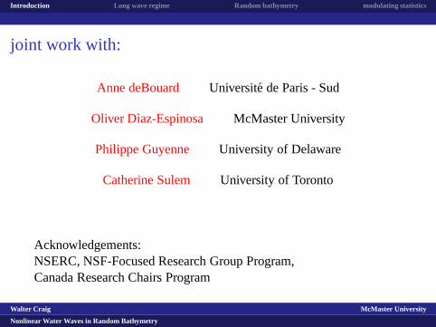
joint work with:
Anne deBouard Universite de Paris - Sud
Oliver Dıaz-Espinosa McMaster University
Philippe Guyenne University of Delaware
Catherine Sulem University of Toronto
Acknowledgements:NSERC, NSF-Focused Research Group Program,Canada Research Chairs Program
Walter Craig McMaster University
Nonlinear Water Waves in Random Bathymetry
Introduction Long wave regime Random bathymetry modulating statistics
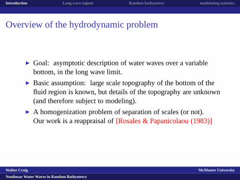
Overview of the hydrodynamic problem
Goal: asymptotic description of water waves over a variablebottom, in the long wave limit.
Basic assumption: large scale topography of the bottom of thefluid region is known, but details of the topography are unknown(and therefore subject to modeling).
A homogenization problem of separation of scales (or not).Our work is a reappraisal of[Rosales & Papanicolaou (1983)]
Walter Craig McMaster University
Nonlinear Water Waves in Random Bathymetry
Introduction Long wave regime Random bathymetry modulating statistics
Overview of the hydrodynamic problem: conclusions
1. Periodic bottom topography; the problem homogenizes fullytogive a KdV equation with effective coefficients[Craig, Guyenne,Nicholls & Sulem (2005)]
2. Random bottom topography given by a stationary ergodicprocess which is mixing,i.e. which decorrelates with spatialdistance.
3. There remainrealization dependent effectsin the equations asimportant as the nonlinearity and the dispersion, given by acanonical processσβ∂XBω(X) (white noise).
4. The solution has bothtransmitted(nonlinear) andscattered(linear) components. Skewness of the statistics of the randomprocess can stabilize or destabilize solutions.
Walter Craig McMaster University
Nonlinear Water Waves in Random Bathymetry
Introduction Long wave regime Random bathymetry modulating statistics
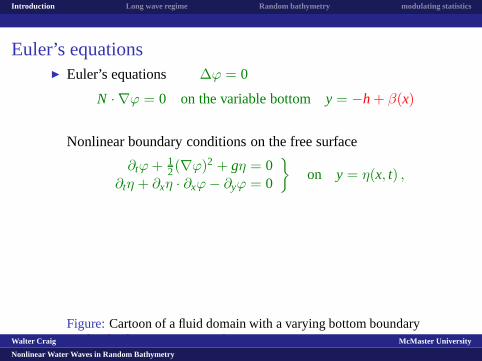
Euler’s equations Euler’s equations ∆ϕ = 0
N · ∇ϕ = 0 on the variable bottom y = −h + β(x)
Nonlinear boundary conditions on the free surface
∂tϕ + 12(∇ϕ)2 + gη = 0
∂tη + ∂xη · ∂xϕ − ∂yϕ = 0
on y = η(x, t) ,
Figure:Cartoon of a fluid domain with a varying bottom boundaryrandomly about a constant valueWalter Craig McMaster University
Nonlinear Water Waves in Random Bathymetry
Introduction Long wave regime Random bathymetry modulating statistics
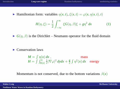
G(η, β) is the Dirichlet – Neumann operator for the fluid domain
Conservation laws
M =∫
η(x) dx , massH =
∫ ∫ ηb(x)
12|∇ϕ|2 dydx+ g
2
∫
η2(x) dx energy
Momentum is not conserved, due to the bottom variationsβ(x)
Walter Craig McMaster University
Nonlinear Water Waves in Random Bathymetry
Introduction Long wave regime Random bathymetry modulating statistics
Scaling regime long wave scaling regime:
X = εx , β(x) = εβ′(X/ε)
εξ′(X) = ξ(x) , ε2η′(X) = η(x)
Hamiltonian for this problem (Boussinesq regime)
H(η′, β′; ε) = (2)12
∫
(h + εβ′(X/ε) − ε2(
β′D tanh(hD)β′)
(X/ε))|DXξ′|2 dX
+12
∫
gη′2 + ε2(ξ′Dη′DXξ′ − h3
3ξ′D4
Xξ′) dX + O(ε3)
Walter Craig McMaster University
Nonlinear Water Waves in Random Bathymetry
Introduction Long wave regime Random bathymetry modulating statistics
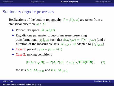
Stationary ergodic processes
Realizations of the bottom topographyβ = β(x, ω) are taken from astatistical ensembleω ∈ Ω
Probability space(Ω,M, P)
Ergodic one parameter group of measure preservingtransformationsτyy∈R such thatβ(x, τyω) = β(x− y, ω) (and afiltration of the measurable sets,My, y ∈ R adapted toτyy∈R)
Case 1:periodicβ(x + p) = β(x)
Case 2:mixing conditions
|P(A∩ τy(B)) − P(A)P(B)| < ϕ(y)√
P(A)P(B) , (3)
for setsA ∈ My≤0 andB ∈ My≥0
Walter Craig McMaster University
Nonlinear Water Waves in Random Bathymetry
Introduction Long wave regime Random bathymetry modulating statistics
Mixing rateIn case 2, we require that the mixing rate satisfy
∫ ∞
0ϕ1/2(y) dy < +∞ (4)
Thevarianceof the processβ(x, ω) is defined to be
σ2β := 2
∫ ∞
0E(β(0, ω)β(0, τyω)) dy ,
LemmaIf β(x, ω) = ∂xγ(x, ω) for some stationary processγ ∈ C1 then
σβ = 0
Walter Craig McMaster University
Nonlinear Water Waves in Random Bathymetry
Introduction Long wave regime Random bathymetry modulating statistics
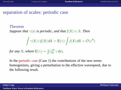
separation of scales: periodic case
TheoremSuppose thatγ(x) is periodic, and thatf (X) ∈ S. Then
∫
γ(X/ε)f (X) dX = E(γ)
∫
f (X) dX + O(εN)
for anyN, whereE(γ) = 1p(
∫ p0 γ dx).
In theperiodic case(Case 1) the contributions of the new termshomogenizes, giving a perturbation to the effective wavespeed, due tothe following result.
Walter Craig McMaster University
Nonlinear Water Waves in Random Bathymetry
Introduction Long wave regime Random bathymetry modulating statistics
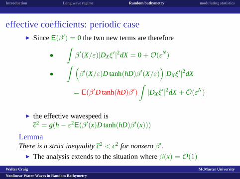
effective coefficients: periodic case SinceE(β′) = 0 the two new terms are therefore
•∫
β′(X/ε)|DXξ′|2dX = 0 + O(εN)
•∫
(
β′(X/ε)D tanh(hD)β′(X/ε))
|DXξ′|2dX
= E(β′D tanh(hD)β′)∫
|DXξ′|2dX + O(εN)
the effective wavespeed isc2 = g(h− ε2E(β′(x)D tanh(hD)β′(x)))
LemmaThere is a strict inequalityc2 < c2 for nonzeroβ′.
The analysis extends to the situation whereβ(x) = O(1)
Walter Craig McMaster University
Nonlinear Water Waves in Random Bathymetry
Introduction Long wave regime Random bathymetry modulating statistics
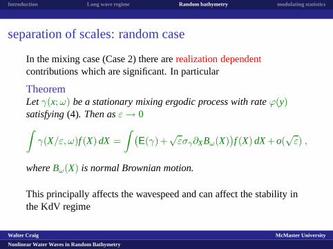
separation of scales: random case
In the mixing case (Case 2) there arerealization dependentcontributions which are significant. In particular
TheoremLetγ(x;ω) be a stationary mixing ergodic process with rateϕ(y)satisfying(4). Then asε → 0∫
γ(X/ε, ω)f (X) dX =
∫
(
E(γ)+√
εσγ∂XBω(X))
f (X) dX+o(√
ε) ,
whereBω(X) is normal Brownian motion.
This principally affects the wavespeed and can affect the stability inthe KdV regime
Walter Craig McMaster University
Nonlinear Water Waves in Random Bathymetry
Introduction Long wave regime Random bathymetry modulating statistics
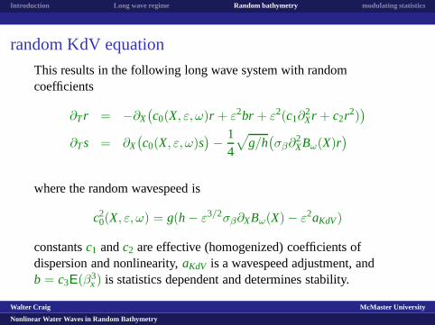
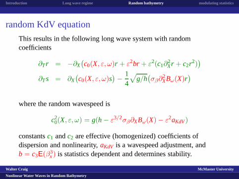
random KdV equation
This results in the following long wave system with randomcoefficients
∂Tr = −∂X(
c0(X, ε, ω)r + ε2br + ε2(c1∂2Xr + c2r2)
)
∂Ts = ∂X(
c0(X, ε, ω)s)
− 14
√
g/h(
σβ∂2XBω(X)r
)
where the random wavespeed is
c20(X, ε, ω) = g(h− ε3/2σβ∂XBω(X) − ε2aKdV)
constantsc1 andc2 are effective (homogenized) coefficients ofdispersion and nonlinearity,aKdV is a wavespeed adjustment, andb = c3E(β3
x) is statistics dependent and determines stability.
Walter Craig McMaster University
Nonlinear Water Waves in Random Bathymetry
Introduction Long wave regime Random bathymetry modulating statistics
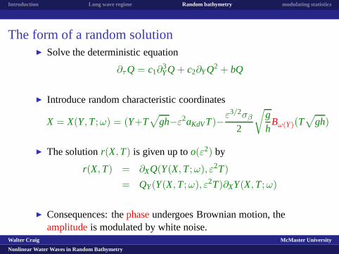
The form of a random solution Solve the deterministic equation
∂τ Q = c1∂3YQ + c2∂YQ2 + bQ
Introduce random characteristic coordinates
X = X(Y, T;ω) = (Y+T√
gh−ε2aKdVT)−ε3/2σβ
2
√
gh
Bω(Y)(T√
gh)
The solutionr(X, T) is given up too(ε2) by
r(X, T) = ∂XQ(Y(X, T;ω), ε2T)
= QY(Y(X, T;ω), ε2T)∂XY(X, T;ω)
Consequences: thephaseundergoes Brownian motion, theamplitudeis modulated by white noise.
Walter Craig McMaster University
Nonlinear Water Waves in Random Bathymetry
Introduction Long wave regime Random bathymetry modulating statistics
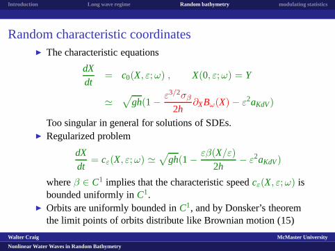
Random characteristic coordinates The characteristic equations
dXdt
= c0(X, ε;ω) , X(0, ε;ω) = Y
≃√
gh(1− ε3/2σβ
2h∂XBω(X) − ε2aKdV)
Too singular in general for solutions of SDEs. Regularized problem
dXdt
= cε(X, ε;ω) ≃√
gh(1− εβ(X/ε)
2h− ε2aKdV)
whereβ ∈ C1 implies that the characteristic speedcε(X, ε;ω) isbounded uniformly inC1.
Orbits are uniformly bounded inC1, and by Donsker’s theoremthe limit points of orbits distribute like Brownian motion (15)
Walter Craig McMaster University
Nonlinear Water Waves in Random Bathymetry
Introduction Long wave regime Random bathymetry modulating statistics
Scattering
The scattered wavefield is solved fors(X, T) by the method ofcharacteristics. SetT′ := T + (X − θ)/
√gh.
s(X, T) = s0(X +√
ghT)
+σβ
4h
∫ X+√
ghT
X∂2
XBω(θ)∂XQ(Y(θ, T′;ω), ε2T′) dθ
Notice the irregularity in the scattered wavefield due to themultiple derivatives of Brownian motion∂2
XBω(X) which interactwith the random solutionr(X, T;ω).
Walter Craig McMaster University
Nonlinear Water Waves in Random Bathymetry
Introduction Long wave regime Random bathymetry modulating statistics
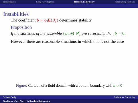
InstabilitiesThe coefficientb = c3E(β3
x) determines stability
PropositionIf the statistics of the ensemble(Ω,M, P) are reversible, thenb = 0
However there are reasonable situations in which this is notthe case
Figure:Cartoon of a fluid domain with a bottom boundary withb > 0
Walter Craig McMaster University
Nonlinear Water Waves in Random Bathymetry
Introduction Long wave regime Random bathymetry modulating statistics
Bottom variations on multiple scales Fluid domains bounded by a bottom with large scale as well as
small scale variations withE(β1(·, X)) = 0
β(x, X, ε, ω) = β0(X, ε) + β1(x, X, ε, ω)
Furthermore, the statistics of the bottom may vary
σ2β1
(X) = 2∫ ∞
0E(β1(0, X;ω)β1(0, X; τyω)) dy
Figure:Cartoon of a fluid domain with a random bottom boundarywith varying statistics
Walter Craig McMaster University
Nonlinear Water Waves in Random Bathymetry
Introduction Long wave regime Random bathymetry modulating statistics
Stationary arrays of mixing processes
TheoremLetγ(x, X;ω) be a smooth (inX) family of stationary mixing ergodicprocesses with uniform mixing rateϕ(y) satisfying(4). Define thelocal variance to be
σ2γ(X) =
∫ ∞
−∞E(γ(·, X;ω)γ(·, X; τyω)) dy
Then asε → 0∫
γ(X/ε, X;ω)f (X) dX =
∫
(
E(γ(·, X))+√
εσγ(X)∂XBω(X))
f (X) dX+o(ε1
whereBω(X) is normal Brownian motion.
Walter Craig McMaster University
Nonlinear Water Waves in Random Bathymetry
Introduction Long wave regime Random bathymetry modulating statistics
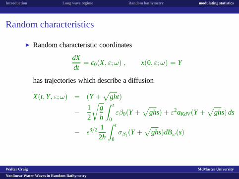
Random characteristics
Random characteristic coordinates
dXdt
= c0(X, ε;ω) , x(0, ε;ω) = Y
has trajectories which describe a diffusion
X(t, Y, ε;ω) = (Y +√
ght)
− 12
√
gh
∫ t
0εβ0(Y +
√
ghs) + ε2aKdV(Y +√
ghs) ds
− ǫ3/2 12h
∫ t
0σβ1(Y +
√
ghs)dBω(s)
Walter Craig McMaster University
Nonlinear Water Waves in Random Bathymetry
Introduction Long wave regime Random bathymetry modulating statistics


![Large-N Quantum Field Theories and Nonlinear Random Processes [ArXiv: 1009.4033 , 1011.2664 ]](https://static.documents.pub/doc/80x56/56812c0e550346895d907b44/large-n-quantum-field-theories-and-nonlinear-random-processes-arxiv-10094033-5685b19b23bb7.jpg)
