Board of Governors of the Federal Reserve System

International Finance Discussion Papers

Number 1013

January 2011

Nonlinearities in the Oil Price-Output Relationship

Lutz Kilian

and

Robert J. Vigfusson

NOTE: International Finance Discussion Papers are preliminary materials circulated to stimulate discussion and critical comment. References in publications to International Finance Discussion Papers (other than an acknowledgment that the writer has had access to unpublished material) should be cleared with the author or authors. Recent IFDPs are available on the Web at www.federalreserve.gov/pubs/ifdp/.

0  

Nonlinearities in the Oil Price-Output Relationship

Lutz Kilian Robert J. Vigfusson

University of Michigan Federal Reserve Board CEPR

November 28, 2010

Abstract: It is customary to suggest that the asymmetry in the transmission of oil price shocks to real output is well established. Much of the empirical work cited as being in support of asymmetries, however, has not directly tested the hypothesis of an asymmetric transmission of oil price innovations. Moreover, many of the papers quantifying these asymmetric responses are based on censored oil price VAR models which recently have been shown to be invalid. Other studies are based on dynamic correlations in the data that do not shed light on the central question of whether the structural responses of real output triggered by positive and negative oil price innovations are asymmetric. Recently, a number of new methodologies have been introduced and applied to the problem of testing and quantifying asymmetric responses of U.S. real economic activity to positive and negative oil price innovations. Our objective is to put this literature in perspective, to contrast it with more traditional approaches, to highlight directions for further research, and to reconcile some seemingly conflicting results reported in the literature. JEL Classification: C32, E37, Q43 Keywords: Oil prices, energy prices, net increase, shocks, propagation, transmission,vector autoregression Acknowledgements: The views in this paper are solely the responsibility of the authors and should not be interpreted as reflecting the views of the Board of Governors of the Federal Reserve System or of any other person associated with the Federal Reserve System. We thank Ron Alquist, Christiane Baumeister, James Hamilton, Ana María Herrera and four anonymous referees for helpful comments. Correspondence to: Lutz Kilian, Department of Economics, 611 Tappan Street, Ann Arbor, MI 48109-1220, USA. Email: lkilian@umich.edu.

1  

1. Introduction

There is an ongoing debate in the macroeconomic literature about whether unexpected increases

in the price of oil cause recessions in oil-importing countries (see, e.g., Kilian 2008; Hamilton

2009). Standard theoretical models of the transmission of exogenous oil price shocks that imply

symmetric responses to oil price increases and decreases cannot explain large declines in

aggregate economic activity in response to positive oil price shocks. In contrast, less

conventional models that imply asymmetries in the response of aggregate real output to positive

and to negative oil price shocks have the ability to explain both larger recessions in response to

unexpected oil price increases and smaller economic expansions in response to unexpected

declines in the price of oil. Proponents of the view that positive oil price shocks have been the

major cause of recessions in the United States therefore inevitably appeal to the presence of

asymmetries in the transmission of oil price shocks. This makes the question of how asymmetric

the responses of real output are to oil price shocks central for the larger question of what lessons

to draw from the historical evidence of the 1970s and 1980s. This question also is paramount

when assessing the effects of major unexpected declines in the price of oil, as occurred in 1986

and 1998, for example, or, more recently, in late 2008.

It is customary to suggest that the asymmetry in the transmission of oil price shocks to

real output is well established. Much of the empirical work cited as being in support of

asymmetries, however, has not directly tested the hypothesis of an asymmetric transmission of

oil price innovations. In fact, many of the papers quantifying these asymmetric responses are

based on precisely the censored oil price VAR methodology that Kilian and Vigfusson (2009)

proved to be invalid. Other studies are based on dynamic correlations in the data that do not shed

light on the central question of whether the structural responses of real output triggered by

positive and negative oil price innovations are asymmetric.

Recently, there has been renewed interest in developing empirical methodologies aimed

at establishing and quantifying asymmetries of the response of real output depending on the sign

of oil price innovations. One problem is how to detect asymmetric response functions. The

problem is not that there have not been earlier attempts to test for asymmetries, but that the

simple diagnostic tests commonly used in the literature dating back to the 1990s are not

informative about the degree of asymmetry of the response functions of real economic activity.

A more suitable impulse-response based test of the null of symmetric response functions has

2  

recently been developed by Kilian and Vigfusson (2009). At the same time, there has been

increasing recognition of the importance of using fully specified structural models in

constructing estimates of asymmetric impulse responses to oil price innovations (see, e.g., Kilian

and Vigfusson 2009, Elder and Serletis 2010). The new econometric models proposed in the

recent literature differ in how much parametric structure they impose in estimating these

response functions. They also tend to produce different empirical results.

Our objective is to put this recent literature in perspective, to contrast it with more

traditional approaches, to highlight directions for further research, and to reconcile some

seemingly conflicting results reported in the literature. The remainder of the paper is organized

as follows. Section 2 reviews the theoretical rationale for asymmetric responses of real economic

activity to oil price shocks. In section 3 we discuss the key modeling choices that affect the

strength of the empirical evidence in favor of asymmetries. Section 4 focuses on the

encompassing regression approach employed by Kilian and Vigfusson (2009) and Herrera,

Lagalo, and Wada (2010) to quantify potentially asymmetric responses. Section 5 reviews the

GARCH-in-mean VAR model designed by Elder and Serletis (2010) to quantify the effect of oil

price uncertainty on real economic activity. Section 6 investigates the related conjecture by

Hamilton (2010) that incorporating asymmetries into joint forecasting models for real GDP

growth and the price of oil helps reduce the out-of-sample mean squared prediction error

(MSPE) of cumulative real GDP growth forecasts. We conclude in Section 7.

2. The Theoretical Rationale for Asymmetric Responses of Real Output

It is useful to review the theoretical rationale for asymmetric responses of real output to oil price

innovations before discussing the empirical evidence. Standard theoretical models of the

transmission of oil price shocks have focused on the implications of fluctuations in the price of

imported crude oil. The most immediate effect of an unexpected increase in the price of imported

crude oil is a reduction in the purchasing power of domestic households, as income is being

transferred abroad. It is important for the argument that it is the price of imported crude oil that

increases because an increase in the price of domestically produced crude oil by itself would

merely cause a redistribution of income rather than a reduction of domestic income in the

aggregate. This direct effect of an increase in the real price of oil imports is symmetric in oil

price increases and decreases. An unexpected increase in the real price of oil will cause

3  

aggregate income to fall by as much as an unexpected decline in the real price of oil of the same

magnitude will cause aggregate income to increase.

The rationale for asymmetric responses of real output to oil price innovations hinges on

the existence of additional indirect effects of unexpected changes in the real price of oil. There

are three main explanations of such effects in the literature. First, it has been stressed that oil

price shocks are relative price shocks that can be viewed as allocative disturbances which cause

sectoral shifts throughout the economy (see, e.g., Hamilton 1988). For example, the case has

been made that reduced expenditures on energy-intensive durables, such as automobiles, in

response to unexpectedly high real oil prices may cause a reallocation of capital and labor away

from the automobile sector. As the dollar value of such purchases may be large relative to the

value of the energy they use, even relatively small changes in the relative price of oil can have

potentially large effects on demand. A similar reallocation may occur within the same sector as

consumers switch toward more energy-efficient durables. If capital and labor are sector specific

or product specific and cannot be moved easily to new uses, these intersectoral and intrasectoral

reallocations will cause labor and capital to be unemployed, resulting in cutbacks in real output

and employment that go beyond the changes in households’ purchasing power triggered by

unexpectedly high oil prices. The same effect may arise if unemployed workers simply wait for

conditions in their sector to improve.

The reallocation effect arises every time the relative price of oil changes unexpectedly,

regardless of the direction of the oil price change. In the case of an unexpected real oil price

increase, the reallocation effect will reinforce the recessionary effects of the loss of purchasing

power, allowing the model to generate a much larger recession than in standard linear models. In

the case of an unexpected real oil price decline, the reallocation effect will partially offset the

increased expenditures driven by the gains in purchasing power, causing a smaller economic

expansion than implied by a linear model. This means that in the presence of a reallocation

effect, the responses of real output to oil are necessarily asymmetric in unanticipated oil price

increases and unanticipated oil price decreases.

The quantitative importance of this channel depends on the extent of expenditure

switching in response to real oil price shocks and on how pervasive frictions in capital and labor

markets are. There is general agreement that the domestic automobile sector is most susceptible

to the reallocation effect. For example, Edelstein and Kilian (2009) have suggested that the

4  

magnitude of the reallocation effect depends primarily on the size of the domestic automobile

industry (as measured by shares in employment and real output) as well as on the extent to which

households substitute imported cars for domestic cars. A more extensive study of the U.S.

automobile sector is provided in Ramey and Vine (2010). Related evidence for the 2007/08

recession has also been presented in Hamilton (2009).

A second explanation of asymmetric response functions focuses on the effects of

uncertainty about the future price of oil on investment decisions. To the extent that the cash flow

from an irreversible investment project depends on the price of oil, real options theory implies

that, all else equal, increased uncertainty about the price of oil causes firms to delay investments,

causing investment expenditures to drop to the extent that unexpected changes in the price of oil

are associated with increased uncertainty about the future price of oil (see, e.g., Bernanke 1983,

Pindyck 1991). As in models of the reallocation effect, the relevant oil price variable in these

models is the real price of oil. Uncertainty in practice is measured by the expected volatility of

the real price of oil over the relevant investment horizon. Exactly the same reasoning applies to

purchases of energy-intensive consumer durables such as cars. Because any unexpected change

in the real price of oil may be associated with higher expected volatility, whether the real price of

oil goes up or down, this uncertainty effect may serve to amplify the effects of unexpected oil

price increases and to offset the effects of unexpected oil price declines, much like the

reallocation effect, resulting in asymmetric responses of real output. The quantitative importance

of this channel depends on how important the real price of oil is for investment and durables

purchase decisions and on the share of such expenditures in aggregate spending. For example, it

seems intuitive that uncertainty about the price of oil would be important for decisions about oil

drilling in Texas, but less obvious that it will be quite as important for other sectors of the

economy such as textile production or information technology.1

A closely related argument has been made in Edelstein and Kilian (2009) who observed

that increased uncertainty about the prospects of staying employed in the wake of unexpected

changes in the real price of oil could cause an increase in precautionary savings (or equivalently

a reduction in consumer expenditures). In this interpretation, uncertainty may affect not merely                                                             1 Bernanke (1983) also suggests that the magnitude of the uncertainty effect will depend on the how certain consumers are about the persistence of changes in the real price of oil. Recent evidence in Anderson, Kellogg and Sallee (2010) based on Michigan consumer survey data, however, suggests that U.S. consumers have consistently employed a no-change forecast of the real price of oil which treats all unexpected changes in the real price of oil as permanent.

5  

energy-intensive consumer durables such as cars, but other consumer expenditures as well. This

argument is logically distinct from the observation that households will smooth their

consumption to the extent that unexpectedly higher real oil prices are associated with an

increased likelihood of becoming unemployed. The key difference is that consumption

smoothing motives are symmetric in unexpected oil price increases and decreases, whereas

precautionary motives are not.

As a third explanation it has been suggested that the response of the Federal Reserve to

oil price shocks is responsible for the depth of the recessions following positive oil price shocks

(see, e.g., Bernanke, Gertler and Watson 1997). The premise is that the Federal Reserve responds

to incipient or actual inflationary pressures associated with unexpected real oil price increases by

raising the interest rate, thereby amplifying the economic contraction. The asymmetry arises

because the Federal Reserve does not respond as vigorously to unexpected declines in the real

price of oil. There is no theoretical model underlying this explanation of asymmetry and indeed

earlier studies have imposed this asymmetry hypothesis in estimation rather than testing it with

the exception of Balke, Brown and Yücel (2002) who concluded that monetary policy alone

cannot account for the asymmetry in the responses of real output. More generally, the notion that

policy makers should respond to oil price shocks in recent years has been shown to be at odds

with economic theory, and the empirical evidence in support of such a link has been shown to be

fragile and to suffer from identification problems and inconsistent estimates (see, e.g., Hamilton

and Herrera 2004; Carlstrom and Fuerst 2006; Herrera and Pesavento 2009, Nakov and Pescatori

2010; Kilian and Lewis 2010).

We conclude that of the three main explanations for asymmetric responses in real output

only the reallocation effect and the uncertainty effect are firmly grounded in economic theory.

Both models imply that an unexpected increase in the real price of oil will cause a negative

response of real output that is larger in absolute terms than the positive response of real output to

an unexpected decline in the real price of oil of the same magnitude. At issue is not so much

whether these theoretical models are correct, but how quantitatively important the asymmetry

implied by these models is for the response of U.S. aggregate real economic activity.

Broadly speaking, there have been two strategies for evaluating these economic models.

One strategy exemplified by Kilian and Vigfusson (2009) has been to specify an econometric

model that can capture asymmetric responses to positive and negative oil price innovations

6  

building on Mork (1989). This approach is not derived from any specific economic model, but

may be used to provide a semiparametric approximation to potentially asymmetric responses

generated by a variety of models. The other strategy has been to model one specific source of

asymmetric responses. A good example is Elder and Serletis (2010), who focus on the

uncertainty effect on real output at the expense of abstracting from other asymmetric

transmission channels. Obviously, the latter approach allows the use of more parametric structure

which helps improve the precision of the estimates and the power of tests of the symmetry null.

On the other hand, it is not clear how to interpret these estimates, if there are multiple sources of

asymmetric responses and the results may be sensitive to the specific parameterization of oil

price uncertainty.

In addition, a number of authors have suggested alternative asymmetric model

specifications that combine asymmetries with additional nonlinearities. The best known example

is the net oil price increase specification of Hamilton (1996, 2003, 2009, 2010). These models

were introduced in recognition of the fact that conventional asymmetric models building on the

distinction between oil price increases and oil price decreases do not appear to fit the U.S. data

(see, e.g., Hooker 1996). The net oil price increase specification has been motivated on the basis

of (untested) behavioral arguments rather than economic theory. A joint test of the asymmetries

and the additional nonlinearities implicit in the approach proposed by Hamilton may be

conducted based on an alternative version of the test proposed by Kilian and Vigfusson (2009).

The approach of Elder and Serletis (2010), in contrast, is not designed to evaluate the

econometric model proposed by Hamilton.

3. Model Specification Issues

There are a number of model specification issues that arise in testing the null hypothesis of

symmetric response functions and in quantifying the degree of asymmetry of the estimated

response functions, regardless of the modeling approach. These modeling choices explain many

of the differences in the empirical results reported in the literature and hence deserve some

discussion.

Which Price of Oil to Use?

Empirical results, for example, can be sensitive to the choice of oil price measure. Leading

candidates for the oil price series include the price of West Texas Intermediate crude oil, the U.S

7  

producer price of crude oil, and the U.S. refiners’ acquisition cost available for imported crude

oil, for domestic crude oil, and for a composite of domestic and imported crude oil. There is no

general consensus on which price of oil to use.

Hamilton (2010) makes the case that, for the purpose of testing for asymmetries in the

transmission of oil price shocks to U.S. real GDP, the U.S. producer price of crude oil is a better

proxy than the refiners’ acquisition cost for imported crude oil because the producer price is

more highly correlated with the price of gasoline. This argument has some merit, but, taking this

argument to its logical conclusion, we should not be using the price of oil at all, but rather the

retail price of gasoline, which itself is a good proxy for the retail price of energy faced by

consumers and firms (see Edelstein and Kilian 2009). This is indeed the approach taken in the

empirical work of Edelstein and Kilian (2009), in Ramey and Vine (2010) and in some of the

results shown in Hamilton (2009).2

On the other hand, traditionally, oil price shocks have been associated with events in the

global oil market. The usual view has been that these foreign shocks were the cause of domestic

economic declines. As discussed in section 2, it is essential for the economic reasoning

underlying the baseline linear model of the transmission of oil price shocks that we focus on the

price of imported crude oil. After all, typical macroeconomic models of the transmission of oil

price shocks are specified in terms of the price of imported crude oil, not the retail price of

gasoline. This line of reasoning suggests that taking the price of imported crude oil as the starting

point, as in Kilian and Vigfusson (2009), also has merits. To illustrate this point consider the

limiting case of an autarchic economy in which all oil is produced domestically. In that case,

there would be no reason to expect aggregate purchasing power to change in response to an

unexpected increase in the price of oil, with the implication that a change in the price of oil of

given magnitude would be equally recessionary, regardless of sign. It would no longer be the

case that unexpected oil price increases are more recessionary than unexpected oil price declines

of the same magnitude.

To further complicate matters, Mork (1989) cautions against the use of the U.S. producer

price of oil favored by Hamilton for a different reason. His concern is that this oil price has been

subject to government regulation and may not be representative of true market prices. Mork

                                                            2 It has been shown that retail gasoline prices may evolve quite differently from the price of crude oil in the short run (see Kilian 2010).

8  

(1989, p. 741) observes that “during the price controls of' the 1970s, this index is misleading

because it reflects only the controlled prices of domestically produced oil. However, since the

price control system closely resembled a combined tax/ subsidy scheme for domestic and

imported crude oil, the marginal cost of crude to U.S. refiners can be approximated by the

composite (for domestic and imported) refiner acquisition cost (RAC) for crude oil.”

Thus, there is unlikely to be one price of oil that is the right choice for all purposes. We

certainly agree with the sentiment in Hamilton (2010) that it is worthwhile to assess the

sensitivity of the test results with respect to alternative oil price measures. To the extent that

different oil price measures yield similar test results, our confidence in these results would

increase. If evidence of asymmetry were to vanish with minor changes in the data, on the other

hand, caution would be called for.

Which Sample Period to Use?

Another important modeling choice is the sample period. Empirical models of the response of

U.S. real output to oil price shocks have been fit on a number of different sample periods with

different results. Understanding which specifications are appropriate and which are not therefore

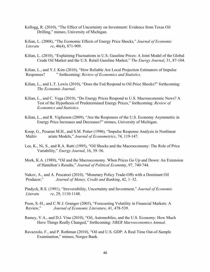
is important. One possibility is to base the model in question on data for the nominal WTI price

of crude oil prior to 1973, as shown in Figure 1. This price series is essentially identical to the

U.S. producer price index for the same period. It is immediately evident that the nominal price of

oil is adjusted only at discrete intervals during that period. As is well known, this pattern is the

result of government regulation. Because the nominal oil price data are generated by a discrete-

continuous choice model, conventional dynamic regressions models are not appropriate for

constructing the responses of real output to oil price shocks during the pre-1973 period. One way

of illustrating this problem is by fitting a random walk model with drift to these data and plotting

randomly generated draws from the fitted model against the actual data. Figure 1 shows one such

sequence. Figure 1 illustrates that the fitted time series model – like any conventional time series

model – is unable to replicate the discontinuous adjustment process underlying the pre-1973

nominal oil price data. This is true even allowing for leptokurtic error distributions. In other

words, standard time series processes are inappropriate for these data and impulse responses

constructed from such models are invalid.

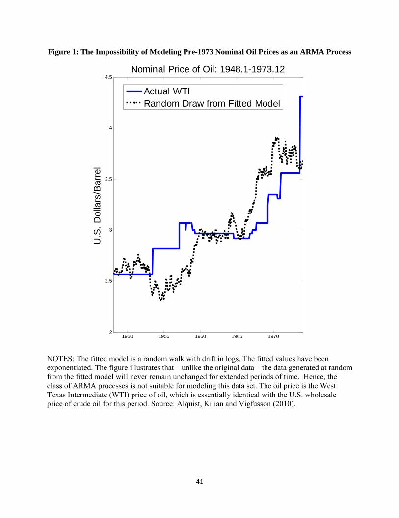
This problem may be ameliorated by deflating the nominal price of oil, which renders the

oil price data continuous and more amenable to VAR analysis. For example, one could fit a

9  

standard time series model to the pre-1973 data shown in the left panel of Figure 2 and construct

the implied responses of real output. Additional problems arise, however, when combining oil

price data generated by a discrete-continuous choice process with oil price data from the post-

1973 era that are fully continuous. This approach is obviously inadvisable when dealing with

nominal oil price data because these data cannot be represented as a standard time series process

for the pre-1973 subsample and are not homogenous over time. Perhaps less obviously, the

approach of combing pre- and post-1973 data is equally unappealing when dealing with dynamic

regressions involving the real price of oil.

The problem is not only that the dynamic process governing the real price of oil is not

homogenous over time, as can be seen by comparing the left and right panels of Figure 2, but

that the nature and speed of the feedback from U.S. macroeconomic aggregates to the real price

of oil differs by construction. For example, it can be shown that the responses to real oil price

innovations are systematically different in pre- and post-1973 data.3 In particular, the real output

responses tend to be systematically larger in pre-1973 data. The same instability arises in the

predictive regressions commonly used to test for lagged nonlinear feedback from the real of price

of oil to real GDP growth (see, e.g., Balke, Brown and Yücel 2002). The p-value for the null

hypothesis that there is no break in 1973.Q4 in the coefficients of this predictive regression is

0.001. Given this evidence of instability, combining pre- and post-1973 real oil price data is not a

valid option. Regression estimates of the relationship between the real price of oil and domestic

macroeconomic aggregates obtained from the entire post-war period are not informative about

the strength of these relationships in post-1973 data.4 It is therefore essential that we restrict the

analysis to the post-1973 period in assessing the evidence for asymmetric real output responses.

This is one point where our views differ from Hamilton (2010) who favors extending the sample

back to 1949.

This point is not just academic. As the analysis in Herrera, Lagalo and Wada (2010)

                                                            3 This result is expected. Hamilton (2003) showed that oil price innovation prior to 1973 were driven by oil supply shocks, whereas Kilian (2008) demonstrated that oil price innovations after 1973 have been dominated by oil demand shocks. Because oil demand and oil supply shocks have different effects on U.S. real GDP the dynamic correlations between oil price innovations and U.S. real GDP growth should be different across these subsamples. 4 This situation is analogous to that of combining real exchange rate data for the pre- and post-Bretton Woods periods in studying the speed of mean reversion toward purchasing power parity. Clearly, the speed of adjustment toward purchasing power parity will differ if one of the adjustment channels is shut down, as was the case under the fixed exchange rate system, than when both prices and exchange rates are free to adjust as was the case under the floating rate system. Thus, regressions on long time spans of real exchange rate data produce average estimates that by construction are not informative about the speed of adjustment in the Bretton Woods system.

10  

illustrates, the evidence of asymmetries using the full sample appears to be driven in large part

by the inclusion of pre-1973 data. Herrera et al. show that there is much less evidence of

asymmetric responses of aggregate industrial production based on post-1973 data, consistent

with the findings for aggregate real GDP in Kilian and Vigfusson (2009) based on post-1973

data. It is, of course, possible that this difference in results merely reflects the reduction in power

from working with a shorter sample, but this does not mean that using pre-1973 data is a valid

option. It is equally possible that this difference in results reflects the structural change in the

underlying time series process in 1973. Either way, the evidence for the post-1973 period is the

only evidence we have to go by and earlier results in the literature based on longer time series

have to be viewed with caution.

Nominal Price of Oil versus Real Price of Oil

Another key difference between existing studies relates to whether the price of oil is specified in

real or in nominal terms. Although an increasing number of empirical studies of the post-1973

data have focused on the real price of oil, many other studies have relied on the nominal price of

oil. One argument sometimes made in support of computing the responses of real output to

nominal price shocks is that in the pre-1973 period the nominal price of oil often remained

frozen for extended periods in which case fluctuations in the real price simply reflect inflation

adjustments that are endogenous to the U.S. economy (see Figures 1 and 2). This means that

innovations in the real price of oil during the pre-1973 period are not necessarily indicative of

exogenous shocks in the oil market. This argument is correct, but does not justify the use of the

nominal price of oil for constructing impulse responses for pre-1973 data because the standard

dynamic regression models from which these responses are computed are not appropriate for

discrete-continuous oil price data, as discussed above. More importantly, it does not justify the

use of the nominal price of oil for the post-1973 period. After 1973, one would expect inflation

innovations to be immediately reflected in the nominal price of oil to the extent that the nominal

price of oil is free to adjust to inflation pressures. As discussed above, this conclusion is more

likely to apply to some oil price measures than to others because of the continued regulation of

the domestic price of oil in the United States. In the absence of regulation, a positive U.S.

monetary disturbance, for example, would be expected to raise the nominal dollar price of oil

and U.S. consumer prices to the same extent, leaving the real price of oil unaffected (see Gillman

and Nakov 2009; Alquist, Kilian and Vigfusson 2010). This argument would hold even if the

11  

nominal price of imported crude oil were set by OPEC. Thus, there is good reason to expect

innovations to the real price of oil in the post-1973 period to reflect real demand and real supply

shocks in the crude oil market.

The focus on real oil price innovations also makes sense because the theoretical models

that imply asymmetries in the transmission of oil price shocks are expressed in terms of the real

price of oil, as discussed in section 2. This is why Kilian and Vigfusson (2009) specified their

model in terms of the real price of oil, as have many other studies including Mork (1989), Lee,

Ni and Ratti (1995), Elder and Serletis (2010), and Herrera, Lagalo and Wada (2010). Hamilton

(2010) makes the counterargument that it is conceivable that consumers of refined oil products

choose to respond to changes in the nominal price of oil rather than the real price of oil, perhaps

because the nominal price of oil is more visible. There is no direct empirical evidence in favor of

this behavioral argument which is at odds with theoretical models of the transmission of oil price

shocks.5 Rather the case for this specification, if there is one, has to be based on the fit of

models estimated at the aggregate level, as in Herrera et al., for example, or on the predictive

success of such models, which explains the emphasis Hamilton (2010) puts on studying

predictive relationships in the data. We will return to this question in section 6.

Nonlinearity versus Asymmetry

Even proponents of using the nominal price in empirical models of the transmission of oil price

shocks have concluded that there is no stable dynamic relationship between percent changes in

the nominal price of oil and in U.S. macroeconomic aggregates. There is evidence from in-

sample fitting exercises, however, of a predictive relationship between suitable nonlinear

transformations of the nominal price of oil and U.S. real output, in particular. The most

successful of these transformations is the net oil price increase measure of Hamilton (2003). Let

ts denote the nominal price of oil in logs and the difference operator. Then the 3-year nominal

                                                            5 Direct evidence in this context refers to microeconomic evidence from structural models at the firm, plant or household level. One example would be evidence of nonlinear adjustment in consumer sentiment in response to oil price innovations. Although Edelstein and Kilian (2009) and Ramey and Vine (2010) have documented adjustments in U.S. consumer sentiment in response to retail energy price innovations, their analysis is based on linear regression models and cannot be used to motivate the use of nonlinear models based on net oil price increases. The same caveat applies to the evidence in Ramey and Vine (2010) on the responses of key indicators for the U.S. automobile industry to various measures of energy price shocks. Both papers transform retail energy price data to allow for time-variation, but the type of nonlinearity considered in these two papers is fundamentally different from that in Mork (1989) or Hamilton (1996, 2003), the focus is on retail energy prices rather than the price of oil, and no allowance is made for asymmetric responses. Thus, this evidence cannot be used as a motivation for using nonlinear models based on net oil price increases.

12  

net oil price increase is defined as: 

, ,3 *max 0, ,net yrt t ts s s

where *ts is the highest oil price in the preceding 3 years. This transformation involves three

distinct ideas. One is that consumers in oil-importing economies respond to increases in the price

of oil only if the increase is large relative to the recent past. If correct, the same logic by

construction should apply to decreases in the price of oil, suggesting a net change transformation

that is symmetric in increases and decreases. The second idea implicit in Hamilton’s definition is

that consumers do not respond to net decreases in the price of oil, allowing us to omit the net

decreases from the model. In other words, consumers respond asymmetrically to net oil price

increases and net oil price decreases and they do so in a very specific fashion. The third idea is

that what matters for the transmission of oil price shocks is the nominal rather than the real price

of oil.

It is important to stress that the net oil price increase is not tightly linked to any of the

theoretical models discussed in section 2, which imply the existence of an asymmetry in the

response of real output to real oil price increases and decreases. First, there is general agreement

that asymmetric model specifications that do not involve the additional nonlinearity proposed by

Hamilton (1996, 2003) such as Mork’s (1989) real oil price increase variable

( 0)t t tr r I r ,

where ( )I denotes the indicator function and tr the log of the real price of oil, are not supported

by the data.6 The additional nonlinear structure embodied in Hamilton’s (2003) net oil price

increase measure, however, is not a feature of the theoretical models discussed in section 2, but

is based on purely behavioral arguments. Second, the theoretical models of section 2 do not

imply that (net) oil price decreases should receive zero weight. They only imply that they should

receive less weight than increases of the same magnitude. Third, the use of the nominal price of

oil is not consistent with economic theory and requires a behavioral motivation. Nevertheless,

Hamilton’s nominal net oil price increase variable has become one of the leading specifications

                                                            6 Although the empirical results in Mork (1989) continue to be cited as evidence of asymmetry, the substance of his results was overturned in Hooker (1996) and Hamilton (1996). Moreover, Kilian and Vigfusson (2009) show that even the original statistical test used by Mork (1989) does not reject the null of symmetric slopes when using data for 1973.II-2007.IV. Qualitatively, similar results are obtained using the recently developed impulse-response based tests.

13  

in the literature on predictive relationships between the price of oil and the U.S. economy.

Hamilton (2010) interprets this relationship as capturing nonlinear changes in consumer

sentiment in response to nominal oil price increases.

The behavioral rationale for the net oil price increase measure, of course, a priori applies

equally to the nominal price of oil and the real price of oil. While Hamilton (2003) applied this

transformation to the nominal price of oil, several other studies have recently explored models

that apply the same transformation to the real price of oil (see, e.g., Kilian and Vigfusson 2009;

Alquist, Kilian, and Vigfusson 2010; Herrera, Lagalo and Wada 2010). In that case, we define

analogously: , ,3 *max 0, .net yr

t t tr r r

Lag Structure

A final question is how many lags to include in the dynamic models used to study the

transmission of oil price shocks. Hamilton (2010) favors more parsimonious models than Kilian

and Vigfusson (2009) with only four quarterly lags. Greater parsimony may make sense in fitting

a predictive model, which is Hamilton’s objective, but makes less sense in estimating the

underlying structural model, which is the objective in Kilian and Vigfusson (2009). Moreover, as

discussed in Hamilton (2010) it is not clear a priori which lag order specification is appropriate

in the context of the Kilian and Vigfusson model. In the current paper, we report results for

models with four lags for ease of comparison. Our main test results based on the real PPI of oil

are essentially identical when using six lags, suggesting that this question is not a central issue.

4. General Tests of the Hypothesis of Symmetric Response Functions

An important question is how to test for the symmetry of the response functions of real output.

Kilian and Vigfusson (2009) proposed a new and conceptually simple impulse-response based

Wald test for this purpose that distinguishes between oil price shocks of different magnitudes and

encompasses all channels of transmission discussed in section 2. This test is built on the

observation that under the null of symmetric response function, the vector of impulse responses

to a positive oil price innovation should be equal to the vector of impulse responses to a negative

oil price innovation except for its sign such that the sum of these vectors is equal to a vector of

zeros. Here we focus on a version of this test designed for models involving the 3-year net oil

price increase.

14  

Slope-Based Tests versus Impulse-Response Based Tests

Kilian and Vigfusson’s approach differs from the traditional approach of conducting a Wald test

of 0 : 0, 1,..., 4,iH i based on the regression:

4 4 4, ,3

1 1 1

net yrt i t i i t i i t i t

i i iy s y s u

, (1)

where ty denotes U.S. real GDP, or an equivalent regression for the real price of oil. Kilian and

Vigfusson’s central point is not that this OLS slope-based test is not powerful enough (indeed

that test tends to reject the null of symmetric slopes, so lack of power is not an obvious concern).

Rather their point is that the slope-based test focuses on the wrong null hypothesis. Testing the

null hypothesis of symmetric response functions requires a test based on impulse responses

rather than slopes. The impulse-response based test proposed in Kilian and Vigfusson (2009) is

superior to traditional tests in that it actually tests the null hypothesis of interest to economists.

The slope-based test does not.

As Kilian and Vigfusson demonstrate using actual data, the impulse-response based test

may reject the null of symmetric response functions, when the null of symmetric slopes is not

rejected; it also may fail to reject the null of symmetric response functions, when the null of

symmetric slopes is rejected. This result is intuitive, given that the impulse responses are highly

nonlinear functions of the slope parameters. Thus, the results of slope-based tests are neither

necessary nor sufficient for testing the symmetry of the impulse-response functions of real

output, and it does not make sense to compare the power of this test with the power of slope-

based tests, except to say that the impulse-response based tests may generate stronger rejections

of symmetry than the slope-based test for the same data, as demonstrated in Herrera, Lagalo and

Wada (2010), for example.

In addition, Kilian and Vigfusson demonstrate that the degree of asymmetry of the

response functions is in general highly dependent on the magnitude of the unexpected change in

the price of oil. It is easily possible, for example, for a linear symmetric model to provide a good

approximation to the response functions except for the most extreme oil price innovations, as we

will illustrate in the next section. Slope-based tests do not distinguish between shocks of

different magnitude, which shows that they are inherently unsuitable for evaluating the degree of

asymmetry of the response functions.

15  

This point illustrates the importance of being explicit about the objective of testing for

asymmetry. Our objective and indeed the explicit objective of the related macroeconomic

literature, as outlined in section 2, has been to test implications of structural models for the

transmission of oil price shocks, as embodied in the model’s structural impulse responses

functions. Using all implications of the structural models in question is appropriate in that

context. Hamilton’s objective, in contrast, is finding out whether there is a predictive relationship

between the price of oil and real GDP. We agree with Hamilton that the nature of this predictive

relationship is a distinct subject from the question of the causal effects of oil price shocks on real

output, but that does not detract from the points made in Kilian and Vigfusson who never

considered the problem of prediction in their paper, but focused on testing the structural

relationships in the data. We will return to the topic of prediction in section 6.

Alternative Tests of the Null of Symmetric Slopes

Although slope-based tests are not designed to assess the degree of asymmetry of the responses

of real output to oil price innovations, they have been used extensively as tests of the null

hypothesis that the data generating process is linear and symmetric. It is therefore useful to

understand the tradeoffs between alternative types of slope-based tests that one might implement.

The most common test in the literature is due to Balke et al. (2002) who proposed testing

0 : 0, 1,..., 4,iH i based on model (1), as discussed earlier. Note that this model includes

regressors not included in the predictive model proposed by Hamilton (2003, 2010): 4 4

, ,3

1 1

net yrt i t i i t i t

i iy y s u

, (1 )

which imposes the restriction 0, 0,i i in estimation. It may seem that we could

alternatively use model (1 ) instead of model (1) to test 0 : 0, 1,..., 4.iH i This test constitutes

the second slope-based test to be included in our comparison.

Yet another slope-based test has recently been proposed by Kilian and Vigfusson (2009).

Their analysis shows that if we start with a structural representation of the data generating

process for real GDP and the price of oil motivated by exactly the same economic reasoning that

led earlier researchers to specify the predictive regression (1), then the dynamic relationship

between the price of oil and real output by construction will include contemporaneous oil price

variables on the right-hand side. This means that under the null of a symmetric structural model

16  

there is an additional restriction that can be imposed in testing. This insight suggests a third

slope-based test that involves fitting 4 4 4

, ,3

0 1 0

net yrt i t i i t i i t i t

i i iy s y s u

(1 )

and testing 0 : 0, 0,..., 4.iH i rather than 0 : 0, 1,..., 4,iH i where we have relied on the

nominal price of oil to maintain notational consistency. Note that model (1 ) follows directly

from the unrestricted fully specified structural model discussed in Kilian and Vigfusson (2009)

and that models (1) and (1 ) can be derived from special cases of this structural model after

imposing additional restrictions.7

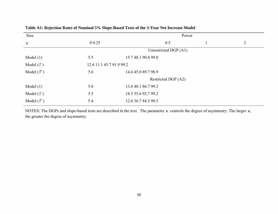
As shown in the appendix, tests based on model (1 ) will suffer from excessive size if the

maintained assumption 0, 0,i i is violated. This size distortion persists asymptotically

because censoring the oil price regressor renders the OLS estimator of i inconsistent except in

the unlikely case that 0, 0.i i Hence, if any 0,i the tests based on models (1) or (1 )

will have more accurate size than the test based on model (1 ). Only if the restriction holds that

there is no feedback at all from oil price declines to real GDP in population (and that there is no

feedback from oil price increases that do not exceed recent peak levels) does the test based on

model (1 ) have accurate size and more power than alternative slope-based tests. Hence, it is

possible for a test based on model (1 ) to generate stronger rejections of the null of symmetric

slopes, but such evidence is equally compatible with a size distortion arising from 0i for some

i and with improved power arising from 0, 0.i i We cannot infer which test is more

appropriate from the empirical results. We can say, however, that economic theory does not

imply that 0, 0.i i The models reviewed in section 2 imply that the feedback from

declines in the real price of oil is weaker than the feedback from increases in the real price of oil,

not that it is zero. Virtually all asymmetric models therefore will be characterized by

0, 0,i i and even small departures from 0, 0,i i will render the OLS estimator of i

inconsistent and misleading (see Kilian and Vigfusson 2009). Nor can this issue be resolved by

statistical testing. The fact that a statistical test of 0 : 0, 0,iH i typically does not reject the

                                                            7 OLS estimation of model (1 ) is based on the premise that the error tu is uncorrelated with .ts This is not an additional assumption, but a direct implication of the existence of a structural model in which the price of energy is predetermined with respect to real GDP. Model (1) does not require that assumption because it is not structural.

17  

null of zero slopes, does not imply that this null is actually true or that it is safe to impose that

restriction in estimation. Hence, in cases when a test based on (1 ) provides stronger rejections

than the other tests on the same data set, it is unclear whether this outcome reflects size

distortions or higher power.

As to the choice between tests based on models (1) and (1 ), it can be shown that the

slope-based test of the joint null of linearity and symmetry based on model (1 ) may have higher

power against departures from 0 : 0,iH 0 ,..., 4,i than the conventional test based on model

(1), which omits the contemporaneous regressors. This point has been illustrated in the context of

Mork’s (1989) asymmetric specification in Kilian and Vigfusson (2009). Depending on the

values of the parameters of the omitted contemporaneous regressors, however, it is also possible

that the test based on model (1) may have higher power than the test based on model (1 ). The

power ranking will differ in general, depending on the data set and model specification. For the

three-year net oil price increase specification studied in the appendix, the test based on model (1)

has slightly higher power, given comparable size.

As expected given this evidence, the differences between using the slope-based tests for

model (1) and for model (1 ) tend to be small for the 3-year net increase specification

considered. In this context, Hamilton (2010) mistakenly claims that the slope-based test based on

model (1 ), as implemented in Kilian and Vigfusson (2009) for the real price of oil, fails to reject

the null of symmetric slopes for real GDP. Hamilton suggests that this test result is at odds with

the rest of the literature and therefore likely to be wrong. Actually, however, Kilian and

Vigfusson found results rather similar to the previous literature. For example, they found no

evidence that the linear model is rejected in favor of the asymmetric model of Mork (1989),

consistent with the substantive findings in Hooker (1996) and Hamilton (1996). Moreover, their

test rejected the linear model at the 5% level in favor of a model including the 3-year net oil

price increase, much like Balke, Brown and Yücel (2002) and Hamilton (2003, 2010) did. In

fact, Kilian and Vigfusson use this example to illustrate the differences between standard slope-

based tests (which reject symmetry in the slopes) and impulse-response based tests (which do not

reject symmetry in the response functions). Thus, Hamilton’s claim that Kilian and Vigfusson

presented evidence based on slope-based tests that the predictive relationship is linear (and his

conclusion that this alleged difference in results is driven by a number of changes in the model

specification relative to previous studies) is not supported by the facts.

18  

This does not mean, of course, that modeling choices such as the choice of sample period

or whether the price of oil is expressed in real or in nominal terms cannot in some cases affect

the degree of statistical significance. We have already discussed each of these modeling choices

in detail. What Hamilton’s (2010) results show is that the rejection of the null of symmetric

slopes reported in Kilian and Vigfusson (2009) is robust to a variety of alternative model

specifications. We agree with Hamilton that given some alternative modeling choices one can

reject the null of symmetric slopes at even higher significance levels than at the 5% level

reported in Kilian and Vigfusson. The rejection decision is the same across all specifications,

however, making this distinction moot.8 More importantly, all of these results are tangential to

the question at hand because the results of slope-based tests are not informative about the degree

of asymmetry in the response functions of real GDP, which is why Kilian and Vigfusson (2009)

caution against the use of any slope-based test, whether the traditional test or the modified test.

They are relevant only to the separate question posed by Hamilton (2010) of whether there is

nonlinear predictability from the price of oil to real GDP growth. There is no way of inferring

“cause” and “effect” from such predictive correlations, of course, which is why we focus on

structural impulse response analysis.

How to Model and Compute Nonlinear Structural Impulse Responses

Hamilton (2010) does not disagree with the conclusion in Kilian and Vigfusson (2009) that

earlier estimates of the responses of real output to oil price shocks were invalid. In fact, he fully

agrees with Kilian and Vigfusson’s point that fundamental changes are needed in the way that

potentially nonlinear models of impulse responses ought to be specified, estimated, and tested.

There are four distinct contributions in Kilian and Vigfusson (2009) that must be viewed

in conjunction. First, Kilian and Vigfusson establish that impulse response estimates from VAR

models involving censored oil price variables are inconsistent even when equation (1) is

correctly specified. Specifically, they demonstrate that asymmetric models of the transmission of

oil price shocks cannot be represented as censored oil price VAR models and are fundamentally

misspecified whether the data generating process is symmetric or asymmetric. This

                                                            8 It should be noted that the three-year net oil price increase specification was originally selected by Hamilton (2003) on the basis of Bayesian model selection methods applied to data that overlap substantially with the sample on which the slope-based test of this specification is based. This introduces an element of data mining that is not reflected in standard asymptotic critical values (see, e.g., Inoue and Kilian 2004). Following the related literature our analysis ignores this caveat.

19  

misspecification renders the parameter estimates inconsistent and inference invalid. Second, they

show that standard approaches to the construction of structural impulse responses used in this

literature are invalid, even when applied to correctly specified models. Instead, Kilian and

Vigfusson proposed a modification of the procedure discussed in Koop, Pesaran and Potter

(1996). Third, Kilian and Vigfusson demonstrate that standard slope-based tests for asymmetry

based on single-equation models are neither necessary nor sufficient for judging the degree of

asymmetry in the structural response functions, which is the question of ultimate interest to users

of these models. Kilian and Vigfusson proposed a direct test of the latter hypothesis which

requires the model to be correctly specified and the nonlinear responses to be correctly

simulated, as discussed in points 1 and 2. Fourth, using this test, they showed empirically that

there is no statistically significant evidence of asymmetry in the response functions for U.S. real

GDP using data for 1973.Q2-2007.Q4.

The Relationship with Balke, Brown and Yücel (2002)

Hamilton’s (2010) discussion may give the impression that the central idea of Kilian and

Vigfusson is already contained in Balke, Brown and Yücel (2002). This is not the case. Balke,

Brown and Yücel certainly deserve credit for being the first researchers to have recognized that

censored oil price VAR models are inherently misspecified, but their solution to this problem is

different from that in Kilian and Vigfusson (2009) in several dimensions. It is important to make

these differences explicit. First, Balke et al. do not explain why impulse response estimates from

censored oil price models are invalid nor do they establish that these estimates are inconsistent,

which helps explain why the use of censored oil price VAR models has remained standard to

this day.9

Second, the structure and the identifying assumptions of Balke et al.’s model differ from

the rest of the literature. Abstracting from nonessential variables, the model used in Balke et al.

can be written as:10

                                                            9 The full extent of their analysis of the problems with censored oil price VAR models is a statement that censored oil price VAR models “are not completely suitable for an examination of asymmetry” and that “it is not at all clear how to interpret a negative Hamilton innovation”. 10 The original specification in Balke et al. included additional macroeconomic aggregates, given their focus on separately identifying monetary policy reactions to the price of oil. For further discussion of this approach see Kilian and Lewis (2010). Under standard identifying assumptions, the inclusion of additional variables in the VAR model does not affect the asymptotic properties of the response of real GDP to oil price innovations, but it may affect the accuracy of the response estimates in small samples. Here we abstract from these small-sample issues and focus on the more fundamental differences between the analysis in Balke et al. (2002) and in Kilian and Vigfusson (2009).

20  

, ,31 11, 12, 1

1 0 1

, ,32 21, 22, 2

1 1 1

p p pnet yr

t i t i i t i i t i ti i i

p p pnet yr

t i t i i t i i t i ti i i

s B s B y s e

y B s B y s e

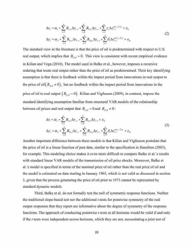
(2)

The standard view in the literature is that the price of oil is predetermined with respect to U.S.

real output, which implies that 12,0 0.B This view is consistent with recent empirical evidence

in Kilian and Vega (2010). The model used in Balke et al., however, imposes a recursive

ordering that treats real output rather than the price of oil as predetermined. Their key identifying

assumption is that there is feedback within the impact period from innovations in real output to

the price of oil 12,0 0 ,B but no feedback within the impact period from innovations in the

price of oil to real output 21,0 0 .B Kilian and Vigfusson (2009), in contrast, impose the

standard identifying assumption familiar from structural VAR models of the relationship

between oil prices and real output that 12,0 0B and 21,0 0 :B

1 11, 12, 11 1

, ,32 21, 22, 2

0 1 0

p p

t i t i i t i ti i

p p pnet yr

t i t i i t i i t i ti i i

r B r B y e

y B r B y r e

(3)

Another important difference between these models is that Kilian and Vigfusson postulate that

the price of oil is a linear function of past data, similar to the specification in Hamilton (2003),

for example. This modeling choice makes it even more difficult to compare Balke et al.’s results

with standard linear VAR models of the transmission of oil price shocks. Moreover, Balke et

al.’s model is specified in terms of the nominal price of oil rather than the real price of oil and

the model is estimated on data starting in January 1965, which is not valid as discussed in section

3, given that the process generating the price of oil prior to 1973 cannot be represented by

standard dynamic models.

Third, Balke et al. do not formally test the null of symmetric response functions. Neither

the traditional slope-based test nor the additional t-tests for pointwise symmetry of the real

output responses that they report are informative about the degree of symmetry of the response

functions. The approach of conducting pointwise t-tests at all horizons would be valid if and only

if the t-tests were independent across horizons, which they are not, necessitating a joint test of

21  

these restrictions that takes account of the covariance terms. Moreover, a joint test also

eliminates the size distortions that arise from the repeated application of t-tests across multiple

horizons which cause spurious rejections of the symmetry null (see, e.g., Kilian and Vega 2010).

For these three reasons, the evidence in Balke et al. cannot be compared directly with the

evidence in Kilian and Vigfusson (2009) and is not dispositive about the degree of asymmetry in

the response functions of U.S. real economic activity to oil price innovations.

The Evidence from Impulse-Response Based Tests

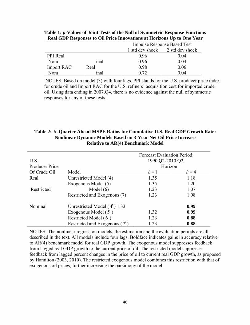
With these clarifications in mind, it is time to focus on the empirical evidence. Table 1 updates

the results in Kilian and Vigfusson (2009) for U.S. real GDP growth. There are a number of

differences in the specification. First, the sample period is set to 1974.Q1-2009.Q4. This takes

account of the structural break in the predictive relationship in 1973.IV and facilitates a clean

comparison of alternative oil price series. Second, for expository purposes we focus on the U.S.

producer price index favored by Hamilton and the U.S. refiners’ acquisition cost for imported

crude oil used in Kilian and Vigfusson (2009). Third, we show results for both the nominal and

real price of oil. Fourth, we focus on a model with four lags rather than the six lags used in

Kilian and Vigfusson (2009). The latter two changes are intended to facilitate the comparison

with Hamilton’s preferred model specification.

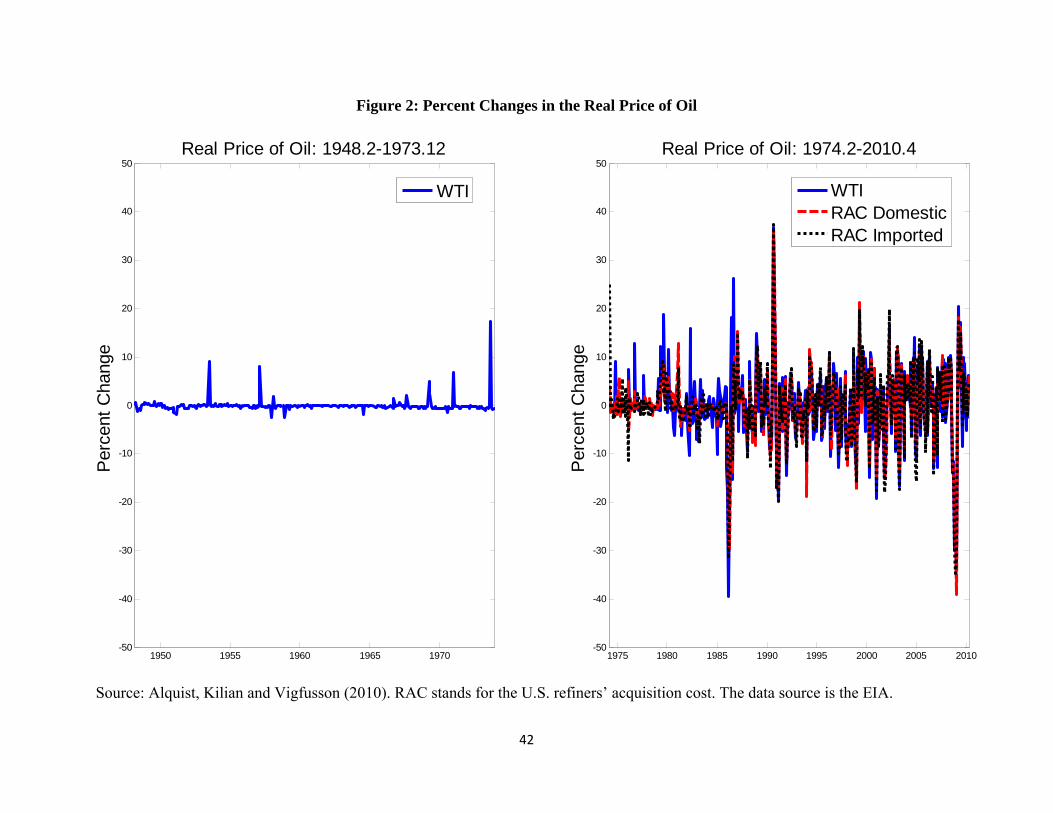
Table 1 shows that there is no statistically significant evidence against the null of

symmetric responses to unexpected oil price increases and unexpected oil price decreases for

shocks of typical magnitude. For the real PPI, for example, the p-value of the impulse-response

based test is 0.90. Qualitatively similar results are obtained whether the price of oil is specified in

real or in nominal terms. The benchmark of one-standard deviation shocks is representative of

about two thirds of all oil price innovations that occurred historically. Only when we focus on

much larger two-standard deviation shocks is there statistically significant evidence of

asymmetry with a p-value of 0.04 for both the real and the nominal PPI. Shocks of this

magnitude or larger have historically occurred with a probability of only 5%. The actual

estimates of the underlying response functions are shown in Figure 3. These estimates have been

normalized such that under the symmetry null the two response functions should coincide

22  

exactly. Similar results are obtained for the refiners’ acquisition cost for crude oil imports.11

The results in Table 1 for two-standard deviation shocks differ from those reported in

Kilian and Vigfusson (2009) for a sample period ending in 2007.Q4. That study found no

evidence against the null of symmetric responses for one- as well as two-standard deviation

shocks. It can be shown that the difference in results is mainly driven by the extended sample

period. As discussed in section 6, there is reason to be cautious in interpreting the post-2007.Q4

results, which are likely to be driven by the financial crisis. If we exclude data after 2007.Q4

from the estimation period, all evidence of asymmetric responses vanishes, even in response to

two-standard deviation shocks.

The analysis for U.S. real GDP growth in Kilian and Vigfusson (2009) has recently been

complemented by additional evidence based on the same impulse-response based test applied to

U.S. industrial production. Herrera, Lagalo and Wada (2010) investigate not only aggregate data,

but industrial production data disaggregated by sector. Their sample period roughly corresponds

to that underlying Table 1. Herrera et al.’s baseline model utilizes the real price of oil.

It is important to understand that a priori there is no reason for the results for industrial

production to match the results for real GDP. One reason is that the share of the service sector in

U.S. real GDP has greatly increased in recent decades. To the extent that the economic models

implying asymmetric responses of real output are designed for the industrial sector, one would

expect weaker evidence of asymmetric responses for aggregate real GDP than for aggregate

industrial production. A second reason is that asymmetric responses may be important at the

sectoral level without necessarily dominating aggregate real economic activity. That is why

disaggregate analysis is valuable in assessing the empirical content of economic models of the

transmission of oil price shocks. At the same time, disaggregate analysis involving a large

number of sectors necessitates the use of critical values that are robust against data mining.

Herrera, Lagalo and Wada (2010) show that there appears to be considerable evidence of

asymmetric responses even after accounting for data mining when the model is estimated on the

full sample including pre-1973 data. That evidence, however, weakens considerably when

discarding the pre-1973 data, as we did in Table 1. The results in Herrera et al. for aggregate

monthly industrial production are remarkably similar to those in Table 1. In both cases, the

                                                            11 Increasing the lag order to six increases the p-values somewhat. For the real PPI, for example, the p-values increase to 0.96 for the one-standard deviation oil price innovation and to 0.15 for the two-standard deviation oil price innovation.

23  

impulse-response based test suggests that there is statistically significant evidence of

asymmetries only in response to very large oil price innovations, but not in response to oil price

innovations of more typical magnitude. Their p-values for responses up to one year are 0.80 and

0.09 compared with 0.90 and 0.04 in Table 1. Thus, the additional evidence for aggregate

industrial production in Herrera, Lagalo and Wada (2010) is broadly consistent with the results

in Table 1 for aggregate real GDP growth.

One important difference is that Herrera et al.’s analysis shows in which sectors the

asymmetry originates. Their results illustrate that the impulse-response based test is powerful

enough to detect departures from the null of symmetric responses to one-standard deviation

shocks within a year. In particular, for oil price innovations of typical magnitude there is no

evidence of asymmetric responses in aggregate industrial production based on , ,3 ,net yrtr but

there is statistically significant evidence (even after accounting for data mining) against the

symmetry null at the disaggregate level for sectors such as chemicals, transit equipment,

petroleum and coal, plastics and rubber, primary metal, and machinery, but interestingly not for

motor vehicles. This evidence confirms that there can be considerable heterogeneity in the degree

of asymmetry across sectors. It suggests that the failure to reject the null of symmetric responses

at the aggregate level may simply mean that asymmetries at the sectoral level are not strong

enough to be detected in the aggregate data.

For oil price innovations corresponding to two-standard deviation shocks, Herrera,

Lagalo and Wada (2010) find somewhat stronger evidence against the null of symmetric

responses, but at the aggregate level the evidence remains somewhat mixed with at best a

marginal rejection at the 10% level at a horizon of one year (not accounting for data mining). At

the disaggregate level, significant rejections are found in sectors such as plastics and rubber,

chemicals and transit equipment, which is to be expected as these industries are known to be

energy intensive, but again not for motor vehicles. None of these rejections for two-standard

deviation shocks is significant after controlling for data mining, however, which may reflect a

loss of power, as large oil price innovations are rare in the data and the resulting responses are

less precisely estimated.

Overall, we conclude that the evidence in favor of asymmetries is mixed. For a one-

standard deviation shock the response functions of U.S. real economic activity appear to be well

approximated by those of a linear symmetric VAR model. This means that the linear symmetric

24  

model can be expected to provide a good approximation in modeling the responses of real output

to innovations in the real price of oil in most situations. For very large innovations in the price of

oil there is evidence that the aggregate responses are asymmetric in that the expansion triggered

by negative oil price innovations is smaller than predicted by a linear model. An interesting

question for future research will be to determine to what extent that asymmetry is associated with

specific expenditure components, building on Edelstein and Kilian (2007, 2009).

It should also be stressed that the nature of the nonlinearity that the impulse-response

based test detects in response to very large oil price innovations is based on the net increase

measure developed by Hamilton (1996, 2003) using purely behavioral arguments. It therefore

does not provide any support for the reallocation effect or the uncertainty effect discussed in

section 2. In fact, if we replaced the net increase measure by a more conventional measure of oil

price increases – as defined in Mork (1989) – that is consistent with economic theory, all

rejections of the symmetry null hypothesis would vanish. Thus, the economic nature of the

apparently asymmetric response to very large oil price innovations remains to be investigated.

One way of approaching this question would be to focus on consumer sentiment data as in

Edelstein and Kilian (2009).

Finally, we have to keep in mind that these test results are tentative only. There are

indications that the evidence in favor of asymmetries in response to large oil price innovations

may be spurious. The sensitivity of the test results to the inclusion of data from the 2008

financial crisis suggests that the evidence in favor of asymmetric responses could reflect

overfitting resulting from the use of a quadratic loss function in conjunction with a relatively

short sample. The concern is that the coincidence of a financial crisis following a large net oil

price increase may cause the model to attribute the effects of the financial crisis on real GDP to

the earlier net oil price increases. Given the unusual decline in real GDP during this episode, the

ability to fit this one episode greatly improves the overall fit of the net increase model. Longer

samples will be required to resolve this question.

5. Tests of the Uncertainty Effect

Although the uncertainty effect has played a prominent role in discussions of asymmetric

responses of real output for two decades, the first study to provide a fully specified model of this

transmission mechanism is Elder and Serletis (2010). In contrast, earlier studies such as Lee, Ni,

25  

and Ratti (1995) and Ferderer (1996) focused on single-equation models of the effect of oil price

uncertainty on real output in which the price of oil is treated as exogenous. That approach is

consistent with theoretical models of the uncertainty effect such as Bernanke (1983) who treats

the price of oil as exogenous with respect to the U.S. economy, but inconsistent with the modern

view that the real price of oil contains an important endogenous component (see Kilian 2008).

Moreover, earlier empirical studies of the uncertainty effect used data from the pre-1973 period,

making the empirical results difficult to interpret.

Elder and Serletis’ baseline model is a VAR(4) model for real GDP growth and the

percent change in the real price of oil with GARCH-in-mean. The oil price measure is the

composite U.S. refiners’ acquisition cost. The model is estimated on post-1974 data. Oil prices

are treated as predetermined with respect to real economic activity. Rather than testing the

symmetry of the response functions directly, as proposed in Kilian and Vigfusson (2009), Elder

and Serletis test the null of no feedback from the one-quarter ahead conditional variance of the

real price of oil in the conditional mean equation. They report that information criteria favor the

model including this term. The presence of GARCH-in-mean effects implies that the response of

real output in this model is asymmetric in unexpected oil price increases and decreases. It also

implies that the degree of asymmetry will in general depend on the magnitude of the shock.

Elder and Serletis report shocks normalized to one standard deviation of the unconditional

distribution of the percent change of the real price of oil (rather than one standard deviation of

the unconditional regression residual).

They provide evidence that increased oil price volatility exacerbates the negative

response of real economic activity to an unexpected increase in the real price of oil, while

dampening the positive response to an unexpected decline in the real price of oil. One of their

striking findings is that the net effect of a unexpected drop in the real price of oil is to cause a

recession. This is not in accordance with the underlying economic theory, which predicts a net

positive effect on real output. Elder and Serletis attribute this result to sampling error. It is

difficult to compare the impulse response estimates in Elder and Serletis to those in Kilian and

Vigfusson because the magnitude of the oil price shock differs and because Elder and Serletis do

not provide a formal test of the symmetry of the response functions, but if we take their point

estimates at face value, there appears to be strong evidence of asymmetric responses.

One possibility is that their results for U.S. real GDP and for U.S. industrial production

26  

are stronger than the results in Kilian and Vigfusson (2009) and Herrera, Lagalo and Wada

(2010) for similar sample periods because their approach is more parametric and therefore has

greater power to detect departures from linearity. A useful exercise for future research would be

to evaluate data generated from the asymmetric model estimated in Elder and Serletis using the

methodology of Kilian and Vigfusson (2009) to determine whether that procedure has the power

to detect the underlying departures from the null of symmetric responses. If it did, this would

cast doubt on the findings in Elder and Serletis. If it did not, the power argument would seem

compelling.

Such a finding would raise the additional question of how plausible it is that the

uncertainty effect is so large. There is reason to be skeptical. The only study to date to provide

formal empirical evidence of an uncertainty effect at the firm level is Kellogg (2010) who

analyzed the investment decisions of oil companies in Texas. Kellogg showed that competitive

oil companies, all else equal, significantly reduce their drilling of oil wells in response to

increased expected oil price volatility. This finding makes sense given the overriding importance

of the price of oil for the cash flow of oil producers. A similar argument may be plausible for

purchases of automobiles, but the share of the automobile sector is relatively small in the U.S.

economy, and more generally energy prices constitute a small determinant of the cash flow of

investment projects. This is clearly an area that deserves further study.

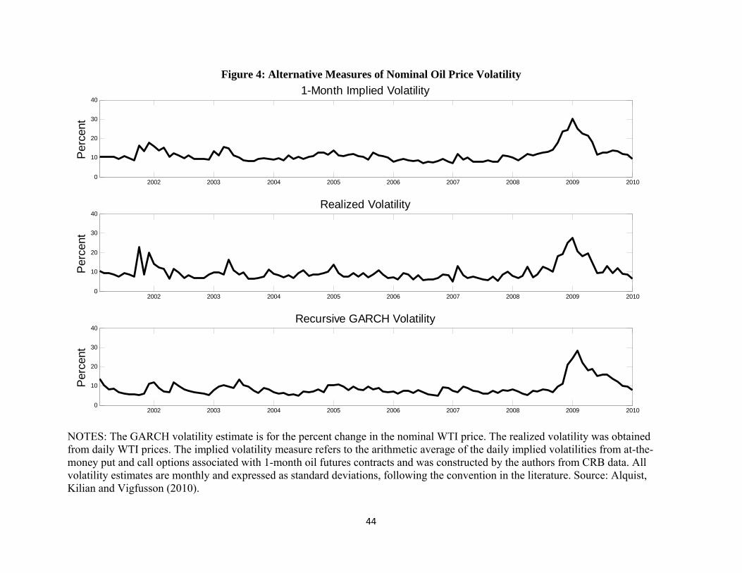
An alternative explanation is that the parametric GARCH-in-mean VAR model is

misspecified. One limitation of this approach, acknowledged by the authors, is that it is not clear

that the conditional variance implied by the GARCH model is the appropriate measure of oil

price uncertainty. To illustrate this point consider three alternative measures of expected oil price

volatility. The upper panel of Figure 4 shows the 1-month implied volatility time series for

2001.1-2009.12, computed from daily CRB data. The next panel plots a realized volatility

estimate constructed from daily percent changes in the nominal WTI price of (see, e.g.,

Bachmeier, Li and Liu 2008). The bottom panel shows the 1-month-ahead conditional variance

obtained from recursively estimated Gaussian GARCH(1,1) models.12

Although all three measures agree that by far the largest volatility peak occurred near the

                                                            12 The initial estimation period is 1974.1-2000.12. The estimates are based on the percent change in the nominal WTI price; the corresponding results for the real WTI price are almost indistinguishable at the 1-month horizon.

27  

end of 2008, there are systematic differences that are likely to affect estimates of the uncertainty

effect. For example, the implied volatility measure peaks in December 2008, whereas GARCH

volatility only peaks in January 2009. This ranking is consistent with the view that implied

volatility is the most forward-looking volatility measure and GARCH volatility the most

backward looking volatility estimate. A similar pattern can be observed during the volatility

spikes of 2001/02 and 2003. On this basis, one would be hard pressed to make the case that

uncertainty about the future price of oil continued to increase in early 2009, as suggested by the

GARCH estimate in Figure 4. Poon and Granger (2003), among others, have shown that implied

volatility typically is a better real time predictor of future price volatility than is GARCH

volatility. The fundamental problem is that GARCH volatility is inherently backward looking,

whereas investors’ expectations tend to be forward looking. Even implied volatility may not be a

good predictor of price volatility, however, given its reliance on oil futures prices which Alquist,

Kilian and Vigfusson (2010) showed to be of limited use in forecasting the price of oil.

Moreover, the assumptions used in constructing implied volatility measures may not hold in

practice.

In addition, a good case can be made that the market’s uncertainty about the future price

of oil may actually fall during sharp oil price declines, making price volatility a poor measure of

the uncertainty about future oil prices. For example, as the OPEC regime collapsed in 1986, the

likelihood of future supply disruptions caused by OPEC evaporated removing a major source of

uncertainty about the future price of oil. There was no reason to extrapolate from the observed

price volatility in 1986 to future volatility if the collapse of OPEC is viewed as a one-time event.

Finally, there is reason to believe that investors in the oil industry respond to the risk that

the real price of oil will fall below a pre-specified level corresponding to the marginal cost of

production rather than to oil price volatility because upside risk in the form of higher oil prices

should not prevent the investment from going ahead. Similarly, investors outside the oil sector

will be primarily concerned with the risk of energy prices rising above a pre-specified level. The

construction of such oil price risk measures is discussed in Alquist, Kilian and Vigfusson (2010).

Clearly, different forms of risk will be relevant for different sectors of the economy suggesting

that generic oil price volatility measures may not be appropriate.

A second and more fundamental concern is that the relevant measure of oil price

volatility in the theoretical models described by Bernanke (1983) and Pindyck (1991) is not the

28  

one-quarter ahead volatility of the real price of oil used by Elder and Serletis. Rather the relevant

volatility measure is the volatility of the real price of oil at horizons relevant to purchase and

investment decisions, which is typically measured in years or even decades rather than days or

months, making all standard measures of short-term price volatility inappropriate. Measuring the

volatility of the real price of oil at longer forecast horizons is inherently difficult given how short

the available time series are, and indeed researchers in practice have typically asserted rather

than measured these shifts in longer-horizon real price volatility. Elder and Serletis (2010)

effectively treat measures of the short-horizon oil price volatility as a proxy for longer-horizon

volatility, which may or may not be appropriate.

One problem with using standard monthly or quarterly GARCH model to quantify

changes in the longer-term expected volatility of the real price of oil is that GARCH forecasts of

the conditional variance quickly revert to their time-invariant unconditional expectation, as the

forecasting horizon increases. If the economically relevant longer-term volatility is constant by

construction, it cannot explain variation in real activity over time. If investment projects take

time to implement before they start generating a cash flow, this weakens and possibly eliminates

the feedback from the current uncertainty to investment decisions.

It may seem that if there is increased uncertainty about the real price of oil that we expect

to be resolved next quarter, then firms affected by this price should necessarily postpone their

investment decisions, even if there is no change in the longer-term oil price uncertainty. Upon

reflection that conclusion is not self-evident. For example, consider a company deciding whether

to build a plant to produce a new SUV. The company’s profits depend on the price of oil in that

demand for this vehicle will decline if the price of oil increases. Suppose that if the company

decides to build the plant today, it will take four quarters to start production and for the cash flow

from selling the SUVs to start. Also take as given that the investment is supposed to amortize

itself within five years. To the extent that our forecast of the conditional variance converges back

to the unconditional variance within four quarters, an unexpected increase in the conditional

variance of the price of oil today will not affect this investment decision (because the cash flow

from the investment that depends on the price of oil does not start within that horizon). More

generally, even if the predictable variation in the conditional variance is more persistent and will

affect expected oil price volatility for a few additional quarters, the overall effect is likely to be

small considering the long horizon for which the cash flow arises (quarters 5 through 24 in the

29  

example) and the tendency for GARCH forecasts of the conditional variance to revert to the

unconditional variance at short horizons.

This reasoning suggests that additional survey data on the distribution of long-run

forecasts and beliefs about future oil prices at long horizons would be helpful in refining tests of

the uncertainty hypothesis.13 Some progress in this direction may be expected from ongoing

work conducted by Anderson, Kellogg and Sallee (2010) based on Michigan survey consumer

expectations of 5-year-ahead gasoline prices.

One could indeed make the case that the GARCH-in-mean model specified by Elder and

Serletis (2010) is more likely to capture the reallocation effect of Hamilton (1988) than the

uncertainty effect of Bernanke (1983) in that it effectively measures volatility in the current real

price of oil (indicative of relative price changes) rather than the expected price of oil at the

horizons relevant to investment decisions. If so, we should be able to show in more detail how

oil price uncertainty affects employment flows at the sectoral, firm and plant level. This is a

question already investigated by Davis and Haltiwanger (2001), except that this earlier work was

based on censored oil price VAR models of the type shown to be invalid in Kilian and Vigfusson

(2009). Further studies using updated time series data and state-of-the-art methods of estimation

and inference appear promising avenues for research.

A third concern with the model specification of Elder and Serletis is that it leaves no

room for other forms of nonlinearity such as the nonlinear adjustment implied by Hamilton’s net

increase measure. If we believe that such nonlinearities matter (or for that matter that there are

other sources of asymmetries not formally modeled), then the GARCH-in-mean VAR model will

be misspecified, making it difficult to determine what the estimated responses of real economic

activity represent.

A final concern is how to reconcile the disaggregate results in Elder and Serletis for U.S.

real consumption with those in Edelstein and Kilian (2009) who showed that a linear symmetric

model does quite well in explaining the historical evolution of U.S. consumption in both 1979

and 1986. One difference is that Edelstein and Kilian (2009) allow for nonlinearities related to

                                                            13 In rare cases, the relevant forecast horizon may be short enough for empirical analysis. For example, Kellogg (2010) makes the case that for the purpose of drilling oil wells in Texas, as opposed to Saudi Arabia, a forecast horizon of only 18 months is adequate. Even at that horizon, however, there are no oil-futures options price data that would allow the construction of implied volatility measures. Kellogg (2010) therefore converts the one-month volatility to 18-month volatilities based on the term structure of oil futures. That approach relies on the assumption that oil futures prices are reliable predictors of future oil prices.

30  

the evolution of the share of energy in consumption, whereas Elder and Serletis do not. Another

difference is that Edelstein and Kilian focused on retail energy prices rather than the price of oil.

An interesting question, considered in ongoing research, is to what extent the apparent

asymmetry in the consumption responses in Elder and Serletis (2010) may be caused by omitted

nonlinearities linked to the time-varying expenditure share on energy or by the choice of the

energy price series.14

6. Out-of-Sample Prediction of Real GDP Growth with Asymmetric Models

The lack of evidence in Kilian and Vigfusson (2009) against the symmetry of the response

functions does not necessarily imply that the reduced-form model is linear or that model (1) is

misspecified. Rather the analysis in Kilian and Vigfusson demonstrates that the outcome of tests

of the symmetry of coefficients in predictive regressions models is not informative about the

degree of asymmetry in the response functions. Hamilton (2010) agrees with Kilian and

Vigfusson as far as impulse response analysis from censored oil price VAR models is concerned,

but suggests that nonlinear models such as model (1) may still be useful for out-of-sample

forecasting. This is a legitimate conjecture that we explore in some detail in this section.

The fundamental difference between impulse response analysis and out-of-sample

forecasting is that in the latter context parsimony may be more important than specifying the

model correctly. Thus, models that are suitable for impulse response analysis need not be

suitable for out-of-sample forecasting. It is important to keep in mind that the question of

whether nonlinear models improve forecast accuracy also is distinct from the question of

whether there is a nonlinear predictive relationship in population, which is the question that

Hamilton (2003) focused on. As is well known, the in-sample fit of nonlinear predictive models

selected using tests such as the slope-based tests discussed earlier does not guarantee gains in

out-of-sample forecast accuracy.

How to construct a suitable nonlinear forecasting model for real GDP growth is still an

open question. Hamilton (2003) suggested that the predictive relationship between oil prices and

U.S. real GDP is nonlinear in that (a) oil price increases matter only to the extent that they

                                                            14 A closely related point has recently been made by Ramey and Vine (2010), who propose to adjust the real price of gasoline for the cost of gasoline shortages induced by regulation. They also consider defining energy price shocks in terms of unanticipated changes in Michigan consumer sentiment regarding car buying conditions. As in Edelstein and Kilian’s work, these adjustments allow us to convert a nonlinear regression relationship into a linear regression model.

31  

exceed the maximum oil price in recent years and that (b) oil price decreases do not matter at all.

This view was based on the in-sample fit of a single-equation predictive model of the form (1 ).

Even granting the presence of such asymmetries in the forecasting model, one point of

contention in the literature is whether the forecasting model should be specified as in Hamilton

(2003), or rather as model (1), as in Balke, Brown and Yücel (2002), for example. The latter

specification encompasses the linear reduced-form model as a special case. Kilian and Vigfusson

prove that dropping the lagged percent changes from model (1) will cause an inconsistency of

the OLS estimates, except in the theoretically implausible case that there is no lagged feedback

from percent changes in the price of oil to real GDP. Hamilton, in contrast, argues in effect that

0, .i i Hamilton (2010) suggests that the potentially misspecified nonlinear predictive

regression model (1 ) that omits the lagged percent changes in the price of oil is preferred for

out-of-sample forecasting given its greater parsimony compared with model (1). Below we

explore the merits of imposing 0, ,i i not only in the context of single-equation models

designed for one-step ahead forecasting, but for multivariate nonlinear dynamic forecasting

models.

A second point of contention is whether nonlinear forecasting models should be specified

in terms of the nominal price of oil or the real price of oil. For linear models, a strong economic

case can be made for using the real price of oil. For nonlinear models, the situation is less clear,

as noted by Hamilton (2010). Because the argument for using net oil price increases is

behavioral, one specification appears as reasonable as the other. Below we therefore consider

models for real as well as nominal oil prices.

A third issue that arises only in constructing iterated forecasts for higher horizons is how

to specify the process governing the price of oil. The case can be made that treating this process

as exogenous with respect to real GDP might help reduce the out-of-sample MSPE, even if that

restriction is incorrect. Below we therefore consider specifications with and without imposing

exogeneity.

In Table 2, we investigate whether there are MSPE reductions associated with the use of

the 3-year net increase in the producer price of crude oil, which is the oil price specification

favored by Hamilton (2003, 2010), at horizons of one and four quarters. In this table, we focus

on models with four lags rather than six lags as in Kilian and Vigfusson’s (2009) impulse

response analysis. This reflects the well-known fact that out-of-sample forecasting in practice

32  

tends to call for greater parsimony than the analysis of population impulse responses. Evaluating

a model designed with one purpose in mind in light of a different objective does not make much

sense. Another reason for choosing four lags for the forecasting model is that it nests the AR(4)

benchmark model for real GDP growth which can be shown to be the most accurate linear

forecasting model. This specification also makes our analysis compatible with Hamilton’s (2003,

2010) preferred model specification for prediction and facilitates direct model comparisons.

Our starting point is an unrestricted multivariate nonlinear forecasting model based on the

real price of oil:

4 4

1 11, 12, 1,1 14 4 4

, ,32 21, 22, 2,

1 1 1

t i t i i t i ti i

net yrt i t i i t i i t i t

i i i

r B r B y e

y B r B y r e

(4)

An analogous nonlinear forecasting model may be constructed based on the nominal price of oil: 4 4

1 11, 12, 1,1 14 4 4

, ,32 21, 22, 2,

1 1 1

t i t i i t i ti i

net yrt i t i i t i i t i t

i i i

s B s B y e

y B s B y s e

( 4 )

In addition, we consider a restricted version of models (4) and ( 4 ) which imposes the

hypothesis that the price of oil is exogenous with respect to real GDP growth 12,( 0, ),iB i

resulting in:

4

1 11, 1,14 4 4

, ,32 21, 22, 2,

1 1 1

t i t i ti

net yrt i t i i t i i t i t

i i i

r B r e

y B r B y r e

(5)

and

4

1 11, 1,14 4 4

, ,32 21, 22, 2,

1 1 1

t i t i ti

net yrt i t i i t i i t i t

i i i

s B s e

y B s B y s e

( 5 )

Alternatively, we may restrict the feedback from lagged percent changes in the price of oil, as

33  

suggested by Hamilton (2003). After imposing 21, 0, ,iB i the baseline nonlinear forecasting

model reduces to:

4 4

1 11, 12, 1,1 14 4

, ,32 22, 2,

1 1

t i t i i t i ti i

net yrt i t i i t i t

i i

r B r B y e

y B y r e

(6)

and 4 4

1 11, 12, 1,1 14 4

, ,32 22, 2,

1 1

t i t i i t i ti i

net yrt i t i i t i t

i i

s B s B y e

y B y s e

  ( 6 )

Finally, we can combine the restrictions 12, 0, ,iB i and 21, 0, ,iB i resulting in the

forecasting models:

4

1 11, 1,14 4

, ,32 22, 2,

1 1

t i t i ti

net yrt i t i i t i t

i i

r B r e

y B y r e

(7)

and 4

1 11, 1,14 4

, ,32 22, 2,

1 1

t i t i ti

net yrt i t i i t i t

i i

s B s e

y B y r e

  ( 7 )

Note that, at the one-quarter horizon, real GDP growth forecasts from model ( 6 ) and ( 7 ) only

depend on the second equation, which is equivalent to using Hamilton’s model (1 ).

All models are estimated recursively by least squares, as is standard in the literature. The

forecasts are constructed by Monte Carlo integration based on 10,000 draws. Our baseline results

employ the PPI used in Hamilton (2003). Additional results for other oil price series and model

specifications are discussed at the end of this section. We start with raw data for January 1974

(which is when the EIA started collecting RAC data) to avoid both the well-documented

structural change in the predictive relationship in late 1973 and to avoid having to make ad hoc

assumptions about backdating the oil price data. This facilitates a clean comparison of alternative

34  

oil price measures and implies that the estimation period starts in 1975.Q2. The initial estimation

period ends in 1990.Q1 (right before the invasion of Kuwait in August of 1990) and the forecast

evaluation ends in 2010.Q2. Table 2 displays the MSPE ratios for all eight models by horizon.

All results are normalized relative to an AR(4) benchmark model for real GDP growth.

The key results can be summarized as follows: First, no nonlinear model in Table 2 is

more accurate than the benchmark AR(4) model at the one-quarter horizon. This includes

Hamilton’s single-equation model (1 ). Second, although model (1 ) performs poorly at the one-

quarter horizon, model ( 7 ) which combines Hamilton’s assumptions with that of exogenous oil

prices and embeds all these assumptions in a multivariate dynamic framework, yields gains in

accuracy relative to the benchmark model at the one-year horizon. The reduction in MSPE is

12%. The main reason for this gain in accuracy is the greater parsimony from omitting the

lagged percent changes in the nominal price of oil; the imposition of exogeneity only plays a

minor role. Third, there are no gains in accuracy relative to the benchmark model from

specifying nonlinear models in the real price of oil, regardless of the additional restrictions

imposed.

An obvious question of interest is to what extent the nonlinearities improve our ability to

forecast major economic downturns in the U.S. In Figure 5 we focus on the model that performs

best in Table 2. The upper panel of Figure 5 shows that the 3-year net oil price increase model

( 7 ) based on the nominal PPI is quite successful in forecasting the downturn of 2008 and the

subsequent recovery four quarters ahead. There are indications, however, that this forecast

success arises for the wrong reasons. In particular, if these forecasts are to be believed, the

financial crisis played almost no role in the economic decline of 2008/09, which does not seem

plausible. Figure 5 illustrates that the net increase model has a tendency to predict major

economic declines anytime the net price of oil increases substantially. In many cases those

predictions proved incorrect. A case in point is the 2005/06 episode. The ability to forecast the

extreme decline of 2008/09, however, under a quadratic loss function more than compensates for

these earlier forecasting errors and accounts for the higher average forecast accuracy of the four-

quarter ahead model. Without that episode, the ranking would be reversed.

The lower panel of Figure 5 shows that the nonlinear model ( 7 ) produces systematically

less accurate forecasts than the AR(4) benchmark model for real GDP growth throughout most of

the evaluation period. By early 2008, very few analysts would have had the courage to stick with

35  

the prediction of a sharp decline in real GDP over the next year, given the previous large forecast

misses of the nonlinear model in 2005-06 and given its persistent underperformance compared

with the AR(4) benchmark model for real GDP growth. Only starting in 2009.Q1, the recursive

MSPE of model ( 7 ) drops below that of the benchmark model, highlighting how sensitive the

results are to one extreme episode in the data. This finding reinforces the concerns with

overfitting we already expressed in section 4 when discussing the in-sample fit of the model.

In Table 2 we focused on the PPI because that is the price upon which Hamilton’s earlier

in-sample analysis in favor of a nonlinear predictive relationship between the price of oil and

U.S. real GDP was based. Table 3 extends the analysis of one-quarter-ahead forecasts to a

variety of oil price measures, alternative lag orders and real as well as nominal prices. A robust

finding across all specifications is that model (1 ) is less accurate out of sample than the AR

model for real GDP growth, except during the recent financial crisis period. This conclusion is

robust to the choice of lag order, to the choice of oil price series, and to the use of nominal or

real oil prices. To the extent that some of the 20 model specifications considered beats the AR

benchmark on the full evaluation sample, this result as well is driven entirely by the financial

crisis episode. Moreover, there is no consistent pattern as to which specifications work well.

Finally, we note that models based on the PPI that appear to fit the data well based on in-sample

predictive analysis (such as then slope-based tests discussed earlier) do not perform well in out-

of-sample forecasting.

Even leaving aside these concerns, it is useful to discuss what we would learn from

evidence of forecasting success. First, forecasting success tells us nothing about the direction of

causality or the transmission of oil price innovations. For example, it is conceivable that the price

of oil as well as U.S. real GDP could be driven by a third variable such as global real activity

(see Ravazzolo and Rothman 2010). Second, the nature of the nonlinearity embodied in the

forecasting model (7 ) and the use of the nominal price of oil cannot be motivated based on the

economic models discussed in section 2. Third, one of the reasons for the apparent success of

some nonlinear forecasting models may very well be the use of information about the long-run.

An interesting question is whether alternative model specifications that embody information

about the long-run would be as successful or perhaps more successful than the class of models

we considered here. Fourth, the fact that the average out-of-sample forecast accuracy is highly

dependent on one episode in the data suggests that the forecast evaluation period may be too

36  

short for reliable rankings.

7. Conclusion

The problem of how to test the null of symmetric responses of U.S. real economic activity to oil

price innovations has been solved only very recently. Kilian and Vigfusson (2009) proposed a

statistical test of this hypothesis based on a class of econometric models that encompasses all

standard theoretical explanations of asymmetric responses or, alternatively, can be modified to

test alternative explanations of asymmetries not based on economic theory. Preliminary evidence

based on these models revealed no evidence against the null of symmetric response functions in

U.S. real GDP data.

Additional results in this paper based on an extended data set that includes observations

until 2009.Q4 showed some evidence of asymmetry in the response of real GDP to very large

shocks, but none in response to shocks of typical magnitude. Herrera, Lagalo and Wada (2010)

provided related evidence for U.S. aggregate industrial production based on the same

econometric approach. Their findings are broadly consistent with the results for real GDP. They

found stronger evidence of asymmetric responses at the sectoral level, however, than in the

aggregate data. In short, the econometric methodology developed in Kilian and Vigfusson

indicates that most of the time the linear symmetric model provides a good approximation in

modeling the responses of real output to innovations in the real price of oil. What evidence for an

asymmetric response there is appears limited to uncommonly large innovations in the real price

of oil. There are indications, however, that even this limited evidence may be spurious. If we

exclude data after 2007.Q4 from the estimation period, all evidence of asymmetric responses

vanishes. The sensitivity of the test result to one very unusual episode in the data may reflect the

use of a quadratic loss function and a relatively short sample. Longer samples will be required to

resolve this question.

In related work, Elder and Serletis (2010) proposed an alternative econometric model that

imposes additional parametric structure in an effort to isolate one of the nonlinear transmission

mechanisms discussed in the literature. As we discussed, this approach has both advantages and

disadvantages compared with the semiparametric approach of Kilian and Vigfusson (2009).

Although the estimates in Elder and Serletis are suggestive of strong asymmetries in the

transmission of oil price innovations, formal tests of the degree of asymmetry of their response

function estimates are not yet available. A natural approach would be to adapt the impulse-

37  

response based test of Kilian and Vigfusson (2009) for this purpose. For now a fair summary of

this empirical literature is that the evidence on the degree of asymmetry of the responses of U.S.

real output may be highly dependent on what parametric structure we impose.

We also investigated the view recently expressed in Hamilton (2010) that we should

focus on the problem of jointly forecasting real GDP growth and the price of oil out-of-sample

rather than testing the structural economic models proposed in the literature. We showed that the

forecasting success of nonlinear asymmetric models depends in general on the model

specification, horizon, and evaluation period. We stressed that there are reasons to be skeptical of

the apparent forecasting success of some nonlinear models of real GDP growth during 2008-10.

For example, we showed that the one-step ahead nonlinear forecasting model favored by

Hamilton (2010) based on extensive in-sample model specification searches is less accurate out

of sample than a linear AR model for real GDP growth, except during the recent financial crisis

period. This conclusion is robust to the choice of lag order, to the choice of oil price series, and

to the use of nominal or real oil prices.

We also noted the difficulties of explaining the forecasting success based on existing

economic models of asymmetries and of giving these results a causal interpretation. In particular,

we cautioned economists against confusing predictive correlations with evidence of “cause” and

“effect” (also see Cooley and LeRoy 1985). The predictive correlations studied by Hamilton

(2003, 2010) in particular do not shed light on the macroeconomic effects of oil price shocks. As

such, we disagree with Hamilton’s (2010) claim that structural impulse responses are simply

conditional forecasts plotted as a function of the horizon.15 Similarly, we need to distinguish

between overall variation in the price of oil and unpredictable variation in the price of oil. A

common misconception is to equate a large cumulative increase in the price of oil with a large oil

price innovation. The consequences of extraordinary events in oil markets can only be studied

with the help of historical decompositions based on structural models, not by inspecting dynamic

                                                            15 In this regard, Hamilton (2010) provides additional evidence based on nonlinear local projections (LP) in the spirit of Jorda (2005, 2009), but his analysis ignores precisely the concerns articulated in Kilian and Vigfusson (2009) that such local projections depend on recent history and on the magnitude of the innovation . The need for Monte Carlo integration methods in these models is also discussed at length in Jorda (2005, p. 168). Moreover, Hamilton’s local projections are not designed to capture structural responses. This would require a consistent estimate of the structural impact multiplier matrix from an external structural model such as the model proposed by Kilian and Vigfusson (see, e.g., Jorda (2009) and Kilian and Kim (2010), equations (5)-(7)). Nor can the slope-based test that Hamilton reports for the LP be interpreted as a test of the symmetry of the impulse response. In short, Hamilton’s LP analysis does not shed any new light on the macroeconomic effects of oil price innovations.

38  

co-movement in the data. There is no substitute for structural econometric modeling in

quantifying possibly nonlinear effects of unexpected oil price shifts.

All three lines of research reviewed in this paper suggest ample opportunities for further

research. Although much progress has been made in recent years in studying asymmetries in the

relationship between the price of oil and U.S. real economic activity, many uncertainties remain.

We conclude that the study of asymmetric effects of oil price innovations on domestic real

activity is likely to remain an active area of research for years to come.

References

Alquist, R., Kilian, L., and R.J. Vigfusson (2010), “Forecasting the Price of Oil,” prepared for: G. Elliott and A. Timmermann (eds.), Handbook of Economic Forecasting, 2, Am sterdam: North-Holland. Anderson, S., Kellogg, R., and J. Sallee (2010), “What Do Consumers Know (or Think They

Know) About the Price of Gasoline?” mimeo, University of Michigan. Bachmeier, L., Li, Q., and D. Liu (2008), “Should Oil Prices Receive So Much Attention? An Evaluation of the Predictive Power of Oil Prices for the US Economy,” Economic Inquiry , 46, 528-539. Balke, N.S., Brown, S.P.A., and M.K. Yücel (2002), “Oil Price Shocks and the U.S. Economy: Where Does the Asymmetry Originate?” Energy Journal, 23, 27‐52. Bernanke, B.S. (1983), “Irreversibility, Uncertainty, and Cyclical Investment,” Quarterly Journal of Economics, 98, 85‐106. Bernanke, B.S., Gertler, M., and M. Watson (1997), “Systematic Monetary Policy and the Effects of Oil Price Shocks,” Brookings Papers on Economic Activity, 1, 91‐142. Carlstrom, C.T., and T.S. Fuerst (2006), “Oil Prices, Monetary Policy and Counterfactual Experim ents,” Journal of Money, Credit and Banking, 38, 1945-1958. Cooley, T.F., and S. LeRoy (1985), “Atheoretical Macroeconometrics: A Critique,” Journal of Monetary Economics, 16, 283-308. Davis, S.J., and J. Haltiwanger (2001), “Sectoral Job Creation and Destruction Responses to Oil Price Changes,” Journal of Monetary Economics, 48, 465-512. Edelstein, P., and L. Kilian (2007), “The Response of Business Fixed Investment to Energy Price Changes: A Test of Some Hypotheses about the Transmission of Energy Price Shocks,” B.E. Journal of Macroeconomics, 7(1). Edelstein, P., and L. Kilian (2009), “How Sensitive are Consumer Expenditures to Retail Energy

39  

Prices?” Journal of Monetary Economics, 56, 766-779. Elder, J., and A. Serletis (2010), “Oil Price Uncertainty,” Journal of Money, Credit and Banking, 42, 1138-1159 Ferderer, J.P. (1996), “Oil Price Volatility and the Macroeconomy: A Solution to the Asymmetry Puzzle,” Journal of Macroeconomics, 18, 1‐16. Gillman, M., and A. Nakov (2009), “Monetary Effects on Nominal Oil Prices,” North American Journal of Economics and Finance, 20, 239-254. Hamilton, J.D. (1988), “A Neoclassical Model of Unemployment and the Business Cycle,” Journal of Political Economy, 96, 593‐617. Hamilton, J. D. (1996). “This is What Happened to the Oil Price–Macroeconomy Relationship,”

Journal of Monetary Economics, 38, 215–220. Hamilton, J. D. (2003) “What is an Oil Shock?” Journal of Econometrics, 113, 363–398. Hamilton, J.D. (2009), “Causes and Consequences of the Oil Shock of 2007-08,” Brookings

Papers on Economic Activity, 1, Spring, 215-261. Hamilton, J.D. (2010), “Nonlinearities and the Macroeconomic Effects of Oil Prices,” forthcoming: Macroeconomic Dynamics. Hamilton, J.D., and A.M. Herrera (2004), “Oil Shocks and Aggregate Economic Behavior: The Role of Monetary Policy: Comment,” Journal of Money, Credit, and Banking, 36, 265 ‐286. Herrera, A.M., Lagalo, L.G., and T. Wada (2010), “Oil Price Shocks and Industrial Production: Is the Relationship Linear?” forthcoming: Macroeconomic Dynamics. Herrera, A.M., and E. Pesavento (2009), “Oil Price Shocks, Systematic Monetary Policy, and the ‘Great Moderation’,” Macroeconomic Dynamics, 13, 107-137. Hooker, M.A. (1996), “What Happened to the Oil Price‐Macroeconomy Relationship?” Journal of Monetary Economics, 38, 195‐213. Inoue, A., and L. Kilian (2004), “In-Sample or Out-of-Sample Tests of Predictability: Which One Should We Use?” Econometric Reviews, 23, 371-402. Jordà, Ò. (2005), “Estimation and Inference of Impulse Responses by Local Projections,” American Economic Review, 95, 161-182. Jordà, Ò. (2009), “Simultaneous Confidence Regions for Impulse Responses,” Review of Economics and Statistics, 91, 629-647.

40  

Kellogg, R. (2010), “The Effect of Uncertainty on Investment: Evidence from Texas Oil Drilling,” mimeo, University of Michigan. Kilian, L. (2008), “The Economic Effects of Energy Price Shocks,” Journal of Economic Literatu re, 46(4), 871-909. Kilian, L. (2010), “Explaining Fluctuations in U.S. Gasoline Prices: A Joint Model of the Global

Crude Oil Market and the U.S. Retail Gasoline Market,” The Energy Journal, 31, 87-104. Kilian, L., and Y.J. Kim (2010), “How Reliable Are Local Projection Estimators of Impulse Responses? ” forthcoming: Review of Economics and Statistics. Kilian, L., and L.T. Lewis (2010), “Does the Fed Respond to Oil Price Shocks?” forthcoming: The Economic Journal. Kilian, L., and C. Vega (2010), “Do Energy Prices Respond to U.S. Macroeconomic News? A

Test of the Hypothesis of Predetermined Energy Prices,” forthcoming: Review of Economics and Statistics.

Kilian, L., and R. Vigfusson (2009), “Are the Responses of the U.S. Economy Asymmetric in Energy Price Increases and Decreases?” mimeo, University of Michigan. Koop, G., Pesaran M.H., and S.M. Potter (1996), “Impulse Response Analysis in Nonlinear Multiv ariate Models,” Journal of Econometrics, 74, 119‐147. Lee, K., Ni, S., and R.A. Ratti (1995), “Oil Shocks and the Macroeconomy: The Role of Price

Variability,” Energy Journal, 16, 39–56. Mork, K.A. (1989), “Oil and the Macroeconomy. When Prices Go Up and Down: An Extension of Hamilton’s Results,” Journal of Political Economy, 97, 740‐744. Nakov, A., and A. Pescatori (2010), “Monetary Policy Trade-Offs with a Dominant Oil Producer,” Journal of Money, Credit and Banking, 42, 1–32. Pindyck, R.S. (1991), “Irreversibility, Uncertainty and Investment,” Journal of Economic Literatu re, 29, 1110‐1148. Poon, S.-H., and C.W.J. Granger (2003), “Forecasting Volatility in Financial Markets: A Review,” Journal of Economic Literature, 41, 478-539. Ramey, V.A., and D.J. Vine (2010), “Oil, Automobiles, and the U.S. Economy: How Much Have Things Really Changed,” forthcoming: NBER Macroeconomics Annual. Ravazzolo, F., and P. Rothman (2010), “Oil and U.S. GDP: A Real Time Out-of-Sample Examination,” mimeo, Norges Bank.

41  

1950 1955 1960 1965 19702

2.5

3

3.5

4

4.5Nominal Price of Oil: 1948.1-1973.12

U.S

. D

olla

rs/B

arre

l

Actual WTIRandom Draw from Fitted Model

Figure 1: The Impossibility of Modeling Pre-1973 Nominal Oil Prices as an ARMA Process

NOTES: The fitted model is a random walk with drift in logs. The fitted values have been exponentiated. The figure illustrates that – unlike the original data – the data generated at random from the fitted model will never remain unchanged for extended periods of time. Hence, the class of ARMA processes is not suitable for modeling this data set. The oil price is the West Texas Intermediate (WTI) price of oil, which is essentially identical with the U.S. wholesale price of crude oil for this period. Source: Alquist, Kilian and Vigfusson (2010).

42  

1950 1955 1960 1965 1970-50

-40

-30

-20

-10

0

10

20

30

40

50Real Price of Oil: 1948.2-1973.12

Per

cent

Cha

nge

1975 1980 1985 1990 1995 2000 2005 2010-50

-40

-30

-20

-10

0

10

20

30

40

50

Per

cent

Cha

nge

Real Price of Oil: 1974.2-2010.4

WTI WTIRAC DomesticRAC Imported

Figure 2: Percent Changes in the Real Price of Oil Source: Alquist, Kilian and Vigfusson (2010). RAC stands for the U.S. refiners’ acquisition cost. The data source is the EIA.

43  

0 1 2 3 4 5 6 7 8-2.5

-2

-1.5

-1

-0.5

0

0.5

Quarters

Per

cent

1 Std Dev Oil Price Innovation

-I(-)I()

0 1 2 3 4 5 6 7 8-2.5

-2

-1.5

-1

-0.5

0

0.5

Quarters

Per

cent

2 Std Dev Oil Price Innovations

-I(-2*)

I(2*)

Figure 3: Responses of Real GDP Based on Innovations in the Real Price of Oil Price U.S. Producer Price Index for Crude Oil

NOTES: The estimation period is 1974.Q1-2009.Q4. All estimates are based on model (3). Similar results are obtained with other oil price measures. ( )I denotes the response function of real GDP to a positive one-standard deviation oil price innovation.

44  

2002 2003 2004 2005 2006 2007 2008 2009 20100

10

20

30

401-Month Implied Volatility

Per

cent

2002 2003 2004 2005 2006 2007 2008 2009 20100

10

20

30

40

Per

cent

Realized Volatility

2002 2003 2004 2005 2006 2007 2008 2009 20100

10

20

30

40Recursive GARCH Volatility

Per

centFigure 4: Alternative Measures of Nominal Oil Price Volatility

NOTES: The GARCH volatility estimate is for the percent change in the nominal WTI price. The realized volatility was obtained from daily WTI prices. The implied volatility measure refers to the arithmetic average of the daily implied volatilities from at-the-money put and call options associated with 1-month oil futures contracts and was constructed by the authors from CRB data. All volatility estimates are monthly and expressed as standard deviations, following the convention in the literature. Source: Alquist, Kilian and Vigfusson (2010).

45  

1992 1994 1996 1998 2000 2002 2004 2006 2008 2010-10

-5

0

5

10

Per

cent

(A

nnua

l Rat

es)

Recursive Forecasts from Nonlinear Model and Realizations

ActualNonlinear Forecast Based on 3-Year Net Oil Price Increase

1992 1994 1996 1998 2000 2002 2004 2006 20080

0.5

1

1.5

2Recursive MSPE Ratio of Nonlinear Model Relative to AR(4) Benchmark

MS

PE

Rat

io

Figure 5: Nonlinear Forecasts from Model ( 7 ) of Cumulative Real GDP Growth Four Quarters Ahead U.S. Producer Price Index for Crude Oil

NOTES: The nonlinear forecasting model is a suitably restricted VAR(4) model for real GDP growth and the percent change in the nominal PPI for crude oil augmented by four lags of the corresponding 3-year nominal net oil price increase. This is the model with the lowest MSPE in Table 2.

46  

Table 1: p-Values of Joint Tests of the Null of Symmetric Response Functions Real GDP Responses to Oil Price Innovations at Horizons Up to One Year

Impulse Response Based Test 1 std dev shock 2 std dev shock PPI Real 0.96 0.04 Nom inal 0.96 0.04 Import RAC Real 0.98 0.06 Nom inal 0.72 0.04

NOTES: Based on model (3) with four lags. PPI stands for the U.S. producer price index for crude oil and Import RAC for the U.S. refiners’ acquisition cost for imported crude oil. Using data ending in 2007.Q4, there is no evidence against the null of symmetric responses for any of these tests.

Table 2: h -Quarter Ahead MSPE Ratios for Cumulative U.S. Real GDP Growth Rate: Nonlinear Dynamic Models Based on 3-Year Net Oil Price Increase

Relative to AR(4) Benchmark Model

U.S. Producer Price

Forecast Evaluation Period: 1990.Q2-2010.Q2 Horizon

Of Crude Oil Model 1h 4h Real Unrestricted Model (4) 1.35 1.18 Exogenous Model (5) 1.35 1.20 Restricted Model (6) 1.23 1.07 Restricted and Exogenous (7) 1.23 1.08 Nominal Unrestricted Model ( 4 ) 1.33 0.99 Exogenous Model (5 ) 1.32 0.99 Restricted Model (6 ) 1.23 0.88 Restricted and Exogenous ( 7 ) 1.23 0.88

NOTES: The nonlinear regression models, the estimation and the evaluation periods are all described in the text. All models include four lags. Boldface indicates gains in accuracy relative to AR(4) benchmark model for real GDP growth. The exogenous model suppresses feedback from lagged real GDP growth to the current price of oil. The restricted model suppresses feedback from lagged percent changes in the price of oil to current real GDP growth, as proposed by Hamilton (2003, 2010). The restricted exogenous model combines this restriction with that of exogenous oil prices, further increasing the parsimony of the model.

47  

Table 3: One-Quarter Ahead MSPE Ratios for U.S. Real GDP Growth Based on Model (1 )

Forecast Evaluation Period 1990.Q2-2007.Q4 1990.Q2-2010.Q2 2008.Q1-2010.Q2 Real Nom inal Real Nom inal Real Nom inal Specification (I) (II) (III) (IV) (V) (VI) MSPE Relative to AR(4) Benchmark Four Lags: Import RAC 1.11 1.22 0.91 1.02 0.50 0.60 Composite RAC 1.50 1.58 1.16 1.26 0.48 0.60 Domestic RAC 1.55 1.50 1.23 1.23 0.57 0.69 PPI 1.63 1.58 1.23 1.23 0.42 0.53 WTI 1.24 1.01 1.04 0.92 0.63 0.74 MSPE Relative to AR(6) Benchmark Six Lags: Import RAC 1.40 1.49 1.10 1.18 0.45 0.52 Composite RAC 2.80 3.30 2.04 2.41 0.47 0.55 Domestic RAC 2.18 2.09 1.66 1.63 0.57 0.66 PPI 2.05 2.11 1.53 1.59 0.43 0.51 WTI 1.32 1.12 1.08 0.97 0.60 0.67

NOTES: Reductions in the MSPE relative to the benchmark are shown in boldface. The estimation period starts in 1975.Q2 and 1975.Q4, respectively, owing to the data constraints discussed earlier. All MSPE ratios are expressed relative to the corresponding AR model for real GDP growth. Model (1 ) is the nonlinear forecasting model favored by Hamilton (2010). In contrast, model (1) estimated using the real import RAC would be the one-step ahead forecasting model implied by structural model employed in Kilian and Vigfusson (2009). For completeness, we note that the recursive MSPE ratio for the latter model with six lags is 1.10 on the evaluation period 1990.Q2-2010.Q2. Hamilton (2010) reports an MSPE ratio of 0.87 for the same model for the evaluation period 1990.Q2-2010.Q2. The difference in result is due to the use of additional pre-1974 data in Hamilton’s regression. It can be shown that after excluding the financial crisis period Hamilton’s regression estimated on his data yields an MSPE ratio of 1.08 and the same regression estimated on our data yields an MSPE ratio of 1.41.

48  

Appendix: The Size and Power Properties of Slope-Based Tests of the Net Increase Model

This appendix compares the size and power properties of three alternative slope-based tests of

the net increase model. We consider two data generating processes. Model (A1) is an

unrestricted multivariate nonlinear forecasting model based on the real price of oil:

4 4

1 11, 12, 1,1 14 4 4

, ,32 21, 22, 2,

0 1 0

t i t i i t i ti i

net yrt i t i i t i i t i t

i i i

r B r B y e

y B r B y r e

(A1)

Model (A2) imposes the additional restrictions of 0 0 and 21, 0 :iB i

4 4

1 11, 12, 1,1 14 4

, ,32 22, 2,

1 1

t i t i i t i ti i

net yrt i t i i t i t

i i

r B r B y e

y B y r e

(A2)

The fact that we focus on the real price of oil rather than the nominal price is immaterial for the

purpose of our simulation study. The data generating processes (DGPs) used in the size

simulations are based on the least-squares parameter estimates obtained from fitting models (A1)

and (A2) to U.S. data after imposing 0. The parameter estimates for the power simulations

are obtained from fitting (A1) and (A2) to the same data after imposing 1. In generating the

pseudo data under the alternative we impose 0.25,0.5,1, 2 . The larger , the greater is the

degree of asymmetry. The innovations in the DGP are treated as Gaussian white noise for

expository purposes. All pseudo data sets are of the same length as the original data.

For each pseudo data set, we employ the three versions of the slope-based test of the null

of symmetry described in section 3. Table A1 summarizes the rejection rates for

0,0.25,0.5,1, 2 . The nominal size is 5%. Under the unrestricted structural DGP, the test

based on model (1 ) suffers from substantial size distortions. It rejects the null of symmetry too

often. The reason for this size distortion is that the OLS estimates of i are inconsistent due to

the censoring of the oil price regressors unless 21, 0 0,iB i as shown in Kilian and Vigfusson

(2009). In other words, these size distortions persist asymptotically. The other two tests have

accurate size because they do not impose that 21, 0, 0.iB i Adjusting for the size distortions of

49  

the test based on model (1 ) has substantially lower power than the other two tests for all 0.

As expected, the size problems of the test based on model (1 ) vanish when considering

the restricted structural DGP (A2). If 21, 0 ,iB i the analysis in Kilian and Vigfusson (2009)

shows that Hamilton’s predictive regression will consistently estimate 0.i i Moreover, the

test based on model (1 ) will be more efficient than a test based on a regression that includes

additional irrelevant regressors, making it more powerful. Table (A1) confirms that for the

restricted DGP all three tests have accurate size, but the test based on model (1 ) has higher

power than the other two tests.

As to the choice between tests based on models (1) and (1 ), Hamilton (2010) argues that

it seems unlikely that another test could have higher power than a test based on (1) because OLS

estimation of the regression model produces asymptotically efficient estimates of the predictive

regression parameters under i.i.d. Gaussian errors. Leaving aside the issue that there is no reason

for the regression errors to be i.i.d. Gaussian in practice, both tests are based on OLS estimation,

so the choice of the estimation method is a non-issue. Instead, what determines the relative

power of tests based on models (1) and (1 ) is the contemporaneous conditional correlation

between the oil price variables and real GDP growth, which may differ for each data set and

model specification. For the specification of interest here, Table A1 suggests that the test based

on model (1) will have slightly higher power than a test based on model (1 ) under both DGPs.

50  

Table A1: Rejection Rates of Nominal 5% Slope-Based Tests of the 3-Year Net Increase Model

Size Power

0 0.25 0.5 1 2

Unrestricted DGP (A1)

Model (1) 5.5 15.7 48.1 90.8 99.0

Model (1 ) 12.6 11.1 45.7 91.9 99.2

Model (1 ) 5.6 14.6 45.0 89.7 98.9

Restricted DGP (A2)

Model (1) 5.6 13.6 40.1 86.7 99.2

Model (1 ) 5.5 18.5 55.6 92.7 99.2

Model (1 ) 5.4 12.6 36.7 84.5 98.5

NOTES: The DGPs and slope-based tests are described in the text. The parameter controls the degree of asymmetry. The larger , the greater the degree of asymmetry.