Hindawi Publishing CorporationDiscrete Dynamics in Nature and SocietyVolume 2008, Article ID 904824, 16 pagesdoi:10.1155/2008/904824

Research ArticleNonlocal Boundary Value Problems forElliptic-Parabolic Differential and DifferenceEquations

Allaberen Ashyralyev1 and Okan Gercek2

1 Department of Mathematics, Fatih University, 34500 Buyukcekmece, Istanbul, Turkey2 Vocational School, Fatih University, 34500 Buyukcekmece, Istanbul, Turkey

Correspondence should be addressed to Okan Gercek, ogercek@fatih.edu.tr

Received 30 June 2008; Accepted 17 September 2008

Recommended by Yong Zhou

The abstract nonlocal boundary value problem −d2u(t)/dt2 + Au(t) = g(t), 0 < t < 1, du(t)/dt −Au(t) = f(t), 1 < t < 0, u(1) = u(−1) + μ for differential equations in a Hilbert space H withthe self-adjoint positive definite operator A is considered. The well-posedness of this problem inHolder spaces with a weight is established. The coercivity inequalities for the solution of boundaryvalue problems for elliptic-parabolic equations are obtained. The first order of accuracy differencescheme for the approximate solution of this nonlocal boundary value problem is presented. Thewell-posedness of this difference scheme in Holder spaces is established. In applications, coercivityinequalities for the solution of a difference scheme for elliptic-parabolic equations are obtained.

Copyright q 2008 A. Ashyralyev and O. Gercek. This is an open access article distributed underthe Creative Commons Attribution License, which permits unrestricted use, distribution, andreproduction in any medium, provided the original work is properly cited.

1. Introduction

It is known that various problems in fluid mechanics and other areas of engineering, physics,and biological systems lead to partial differential equations of variable types. Methods ofsolutions of nonlocal boundary value problems for partial differential equations of variabletype have been studied extensively by many researchers (see, e.g., [1–4] and the referencesgiven therein).

The nonlocal boundary value problem

−d2u(t)dt2

+Au(t) = g(t), 0 < t < 1,

du(t)dt

−Au(t) = f(t), −1 < t < 0,

u(1) = u(−1) + μ

(1.1)

2 Discrete Dynamics in Nature and Society

for differential equations in a Hilbert spaceH with the self-adjoint positive definite operatorA is considered.

Let us denote by Cα0,1([−1, 1],H), 0 < α < 1 the Banach space obtained by completion

of the set of all smoothH-valued function ϕ(t) on [−1, 1] in the norm

‖ϕ‖Cα0,1([−1,1],H) = ‖ϕ‖C([−1,1],H) + sup

−1<t<t+τ<0

(−t)α‖ϕ(t + τ) − ϕ(t)‖Hτα

+ sup0<t<t+τ<1

(1 − t)α(t + τ)α‖ϕ(t + τ) − ϕ(t)‖Hτα

,

(1.2)

and denote by Cα0,1([0, 1],H), 0 < α < 1 the Banach space obtained by completion of the set

of all smoothH-valued function ϕ(t) on [0, 1] in the norm

‖ϕ‖Cα0,1([0,1],H) = ‖ϕ‖C([0,1],H) + sup

0<t<t+τ<1

(1 − t)α(t + τ)α‖ϕ(t + τ) − ϕ(t)‖Hτα

, (1.3)

finally denote by Cα0 ([−1, 0],H), 0 < α < 1 the Banach space obtained by completion of the

set of all smoothH-valued function ϕ(t) on [−1, 0] in the norm

‖ϕ‖Cα0 ([−1,0],H) = ‖ϕ‖C([−1,0],H) + sup

−1<t<t+τ<0

(−t)α‖ϕ(t + τ) − ϕ(t)‖Hτα

. (1.4)

Here C([a, b],H) stands for the Banach space of all continuous functions ϕ(t) defined on[a, b]with values inH equipped with the norm

||ϕ||C([a,b],H) = maxa≤t≤b

‖ϕ(t)‖H. (1.5)

A function u(t) is called a solution of problem (1.1) if the following conditions are satisfied.

(i) u(t) is twice continuously differentiable on the segment (0, 1] and continuouslydifferentiable on the segment [−1, 1]; the derivatives at the endpoints of the segmentare understood as the appropriate unilateral derivatives.

(ii) The element u(t) belongs to the domain D(A) of A for all t ∈ [−1, 1], and thefunction Au(t) is continuous on the segment [−1, 1].

(iii) u(t) satisfies the equations and the nonlocal boundary condition (1.1).

A solution of problem (1.1) defined in this manner will henceforth be referred to as asolution of problem (1.1) in the space C(H) = C([−1, 1],H).

We say that problem (1.1) is well-posed in C(H), if there exists a unique solution u(t)in C(H) of problem (1.1) for any g(t) ∈ C([0, 1],H), f(t) ∈ C([−1, 0],H), and μ ∈ D(A), andthe following coercivity inequality is satisfied:

‖u′′‖C([0,1],H) + ‖u′‖C([−1,0],H) + ‖Au‖C(H) ≤M[‖g‖C([0,1],H) + ‖f‖C([−1,0],H) + ‖Aμ‖H], (1.6)

whereM is independent of μ, f(t), and g(t).

A. Ashyralyev and O. Gercek 3

Problem (1.1) is not well-posed in C(H) [5]. The well-posedness of the boundaryvalue problem (1.1) can be established if one considers this problem in certain spaces F(H)of smoothH-valued functions on [−1, 1].

A function u(t) is said to be a solution of problem (1.1) in F(H) if it is a solution of thisproblem in C(H) and the functions u′′(t) (t ∈ 0, 1]), u′(t) (t ∈ −1, 1]) and Au(t) (t ∈ −1, 1])belong to F(H).

As in the case of the space C(H), we say that problem (1.1) is well-posed in F(H), ifthe following coercivity inequality is satisfied:

‖u′′‖F([0,1],H) + ‖u′‖F([−1,0],H) + ‖Au‖F(H) ≤M[‖g‖F([0,1],H) + ‖f‖F([−1,0],H) + ‖Aμ‖H

], (1.7)

whereM is independent of μ, f(t), and g(t).If we set F(H) equal to Cα

0,1(H) = Cα0,1([−1, 1],H) (0 < α < 1), then we can establish

the following coercivity inequality.

Theorem 1.1. Suppose μ ∈ D(A). Then the boundary value problem (1.1) is well-posed in a Holderspace Cα

0,1(H) and the following coercivity inequality holds:

‖u′′‖Cα0,1([0,1],H) + ‖u′‖Cα

0 ([−1,0],H) + ‖Au‖Cα0,1(H)

≤M[

1α(1 − α)

[‖f‖Cα

0 ([−1,0],H) + ‖g‖Cα0,1([0,1],H)

]+ ‖Aμ‖H

].

(1.8)

HereM is independent of f(t), g(t), and μ.

The proof of this assertion follows from the scheme of the proof of the theorem onwell-posedness of paper [5] and is based on the following formulas:

u(t) =(I − e−2A1/2

)−1[(e−tA

1/2 − e−(−t+2)A1/2)u0

+(e−(1−t)A

1/2 − e−(t+1)A1/2)u1]+(I − e−2A1/2

)−1

×(e−(1−t)A

1/2 − e−(t+1)A1/2)∫1

0A−1/22−1

(e−(1−s)A

1/2 − e−(s+1)A1/2)g(s)ds

−∫1

0A−1/22−1

(e−(t+s)A

1/2 − e−|t−s|A1/2)g(s)ds, 0 ≤ t ≤ 1,

u(t) = etAu0 +∫ t

0e(t−s)Af(s)ds, −1 ≤ t ≤ 0,

u0 =(I + e−2A

1/2+A1/2

(I − e−2A1/2

)− 2e−(A

1/2+A))−1

×[e−A

1/2[2∫−1

0e−(1+s)Af(s)ds +

∫1

0A−1/2

(e−(1−s)A

1/2 − e−(s+1)A1/2)g(s)ds

]+ 2e−A

1/2μ

]

+(I − e−2A1/2

)(I + e−2A

1/2+A1/2

(I − e−2A1/2

)− 2e−(A

1/2+A))−1

×[−A−1/2f(0) +

∫1

0A−1/2e−sA

1/2g(s)ds

]

(1.9)

4 Discrete Dynamics in Nature and Society

for the solution of problem (1.1) and on the estimates

∥∥∥(I − e−2A1/2

)−1∥∥∥H→H

≤M,

∥∥∥(I + e−2A

1/2+A1/2

(I − e−2A1/2

)− 2e−(A

1/2+A))−1∥∥∥

H→H≤M,

∥∥∥A1/2(I + e−2A

1/2+A1/2

(I − e−2A1/2

)− 2e−(A

1/2+A))−1∥∥∥

H→H≤M,

∥∥∥(A1/2)αe−tA1/2∥∥∥H→H

≤ t−α, t > 0, 0 ≤ α ≤ 1,

‖Aαe−tA||H→H ≤ t−α, t > 0, 0 ≤ α ≤ 1.

(1.10)

Remark 1.2. The nonlocal boundary value problem for the elliptic-parabolic equation

du(t)dt

+Au(t) = f(t), 0 < t < 1,

−d2u(t)dt2

+Au(t) = g(t), −1 < t < 0,

u(1) = u(−1) + μ

(1.11)

in a Hilbert space H with a self-adjoint positive definite operator A is considered in paper[6]. The well-posedness of this problem in Holder spaces Cα(H) without a weight wasestablished under the strong condition on μ.

Now, the applications of this abstract results are presented.First, the mixed boundary value problem for the elliptic-parabolic equations

ga − utt − (a(x)ux)x + δu = g(t, x), 0 < t < 1, 0 < x < 1,

ut + (a(x)ux)x − δu = f(t, x), −1 < t < 0, 0 < x < 1,

u(t, 0) = u(t, 1), ux(t, 0) = ux(t, 1), −1 ≤ t ≤ 1,

u(1, x) = u(−1, x) + μ(x), 0 ≤ x ≤ 1,

u(0+, x) = u(0−, x), ut(0+, x) = ut(0−, x), 0 ≤ x ≤ 1

(1.12)

is considered. Problem (1.12) has a unique smooth solution u(t, x) for a(x) ≥ a > 0 (x ∈(0, 1)), and g(t, x) (t ∈ 0, 1], x ∈ [0, 1]), f(t, x) (t ∈ [−1, 0], x ∈ 0, 1]) the smooth functions andδ = const > 0. This allows us to reduce the mixed problem (1.12) to the nonlocal boundaryvalue problem (1.1) in the Hilbert space H = L2[0, 1] with a self-adjoint positive definiteoperator A defined by (1.12).

A. Ashyralyev and O. Gercek 5

Theorem 1.3. The solutions of the nonlocal boundary value problem (1.12) satisfy the coercivityinequality

‖utt‖Cα0,1([0,1],L2[0,1]) + ‖ut‖Cα

0 ([−1,0],L2[0,1]) + ‖u‖Cα0,1([−1,1],W2

2 [0,1])

≤M[

1α(1 − α)

[‖g‖Cα

0,1([0,1],L2[0,1]) + ‖f‖Cα0 ([−1,0],L2[0,1])

]+ ‖μ‖W2

2 [0,1]

],

(1.13)

whereM is independent of f(t, x), g(t, x), and μ(x).

The proof of Theorem 1.3 is based on the abstract Theorem 1.1 and the symmetryproperties of the space operator are generated by problem (1.12).

Second, letΩ be the unit open cube in the n-dimensional Euclidean space Rn (0 < xk <

1, 1 ≤ k ≤ n)with boundary S, Ω = Ω ∪ S. In [−1, 1] ×Ω, the boundary value problem for themultidimensional elliptic-parabolic equation

−utt −n∑

r=1

(ar(x)uxr )xr = g(t, x), 0 < t < 1, x ∈ Ω,

ut +n∑

r=1

(ar(x)uxr )xr = f(t, x), −1 < t < 0, x ∈ Ω,

u(t, x) = 0, x ∈ S, − 1 ≤ t ≤ 1; u(1, x) = u(−1, x) + μ(x), x ∈ Ω,

u(0+, x) = u(0−, x), ut(0+, x) = ut(0−, x), x ∈ Ω

(1.14)

is considered. Problem (1.14) has a unique smooth solution u(t, x) for ar(x) ≥ a > 0 (x ∈ Ω)and g(t, x) (t ∈ (0, 1), x ∈ Ω), f(t, x) (t ∈ (−1, 0), x ∈ Ω), the smooth functions. This allowsus to reduce the mixed problem (1.14) to the nonlocal boundary value problem (1.1) in theHilbert space H = L2(Ω) of all the integrable functions defined on Ω, equipped with thenorm

‖f‖L2(Ω) ={∫

· · ·∫

x∈Ω|f(x)|2dx1 · · ·dxn

}1/2

(1.15)

with a self-adjoint positive definite operator A defined by (1.14).

Theorem 1.4. The solution of the nonlocal boundary value problem (1.14) satisfies the coercivityinequality

‖utt‖Cα0,1([0,1],L2(Ω)) + ‖ut‖Cα

0 ([−1,0],L2(Ω)]) + ‖u‖Cα0,1([−1,1],W2

2 (Ω))

≤M[

1α(1 − α)

[‖g‖Cα

0,1([0,1],L2(Ω)) + ‖f‖Cα0 ([−1,0],L2(Ω))

]+ ‖μ‖W2

2 (Ω)

],

(1.16)

whereM is independent of f(t, x), g(t, x), and μ(x).

6 Discrete Dynamics in Nature and Society

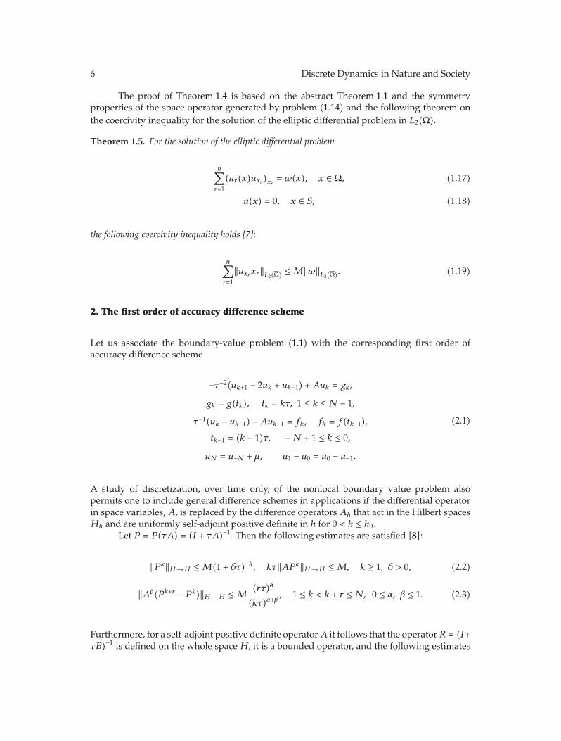
The proof of Theorem 1.4 is based on the abstract Theorem 1.1 and the symmetryproperties of the space operator generated by problem (1.14) and the following theorem onthe coercivity inequality for the solution of the elliptic differential problem in L2(Ω).

Theorem 1.5. For the solution of the elliptic differential problem

n∑

r=1

(ar(x)uxr )xr = ω(x), x ∈ Ω, (1.17)

u(x) = 0, x ∈ S, (1.18)

the following coercivity inequality holds [7]:

n∑

r=1

‖uxrxr‖L2(Ω) ≤M||ω||L2(Ω). (1.19)

2. The first order of accuracy difference scheme

Let us associate the boundary-value problem (1.1) with the corresponding first order ofaccuracy difference scheme

−τ−2(uk+1 − 2uk + uk−1) +Auk = gk,

gk = g(tk), tk = kτ, 1 ≤ k ≤N − 1,

τ−1(uk − uk−1) −Auk−1 = fk, fk = f(tk−1),

tk−1 = (k − 1)τ, −N + 1 ≤ k ≤ 0,

uN = u−N + μ, u1 − u0 = u0 − u−1.

(2.1)

A study of discretization, over time only, of the nonlocal boundary value problem alsopermits one to include general difference schemes in applications if the differential operatorin space variables, A, is replaced by the difference operators Ah that act in the Hilbert spacesHh and are uniformly self-adjoint positive definite in h for 0 < h ≤ h0.

Let P = P(τA) = (I + τA)−1. Then the following estimates are satisfied [8]:

‖Pk‖H→H ≤M(1 + δτ)−k, kτ‖APk‖H→H ≤M, k ≥ 1, δ > 0, (2.2)

‖Aβ(Pk+r − Pk)‖H→H ≤M (rτ)α

(kτ)α+β, 1 ≤ k < k + r ≤N, 0 ≤ α, β ≤ 1. (2.3)

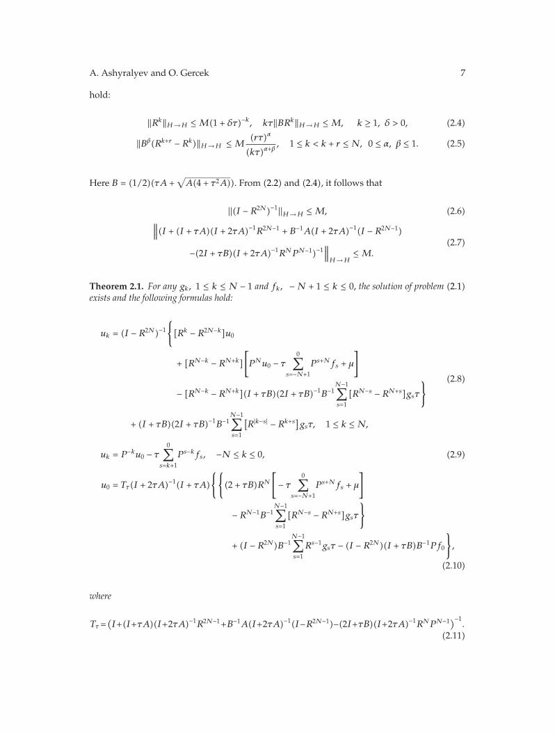
Furthermore, for a self-adjoint positive definite operatorA it follows that the operatorR = (I+τB)−1 is defined on the whole spaceH, it is a bounded operator, and the following estimates

A. Ashyralyev and O. Gercek 7

hold:

‖Rk‖H→H ≤M(1 + δτ)−k, kτ‖BRk‖H→H ≤M, k ≥ 1, δ > 0, (2.4)

‖Bβ(Rk+r − Rk)‖H→H ≤M (rτ)α

(kτ)α+β, 1 ≤ k < k + r ≤N, 0 ≤ α, β ≤ 1. (2.5)

Here B = (1/2)(τA +√A(4 + τ2A)). From (2.2) and (2.4), it follows that

||(I − R2N)−1||H→H ≤M, (2.6)∥∥∥(I + (I + τA)(I + 2τA)−1R2N−1 + B−1A(I + 2τA)−1(I − R2N−1)

−(2I + τB)(I + 2τA)−1RNPN−1)−1∥∥∥H→H

≤M.(2.7)

Theorem 2.1. For any gk, 1 ≤ k ≤ N − 1 and fk, −N + 1 ≤ k ≤ 0, the solution of problem (2.1)exists and the following formulas hold:

uk = (I − R2N)−1{

[Rk − R2N−k]u0

+ [RN−k − RN+k]

[

PNu0 − τ0∑

s=−N+1

Ps+Nfs + μ

]

− [RN−k − RN+k](I + τB)(2I + τB)−1B−1N−1∑

s=1

[RN−s − RN+s]gsτ

}

+ (I + τB)(2I + τB)−1B−1N−1∑

s=1

[R|k−s| − Rk+s]gsτ, 1 ≤ k ≤N,

(2.8)

uk = P−ku0 − τ0∑

s=k+1

Ps−kfs, −N ≤ k ≤ 0, (2.9)

u0 = Tτ(I + 2τA)−1(I + τA)

{{

(2 + τB)RN

[

− τ0∑

s=−N+1

Ps+Nfs + μ

]

− RN−1B−1N−1∑

s=1

[RN−s − RN+s]gsτ

}

+ (I − R2N)B−1N−1∑

s=1

Rs−1gsτ − (I − R2N)(I + τB)B−1Pf0

}

,

(2.10)

where

Tτ =(I+(I+τA)(I+2τA)−1R2N−1+B−1A(I+2τA)−1(I−R2N−1)−(2I+τB)(I+2τA)−1RNPN−1)−1.

(2.11)

8 Discrete Dynamics in Nature and Society

Proof. By [8, 9],

uk = (I − R2N)−1{

[Rk − R2N−k]ξ + [RN−k − RN+k]ψ

− [RN−k − RN+k](I + τB)(2I + τB)−1B−1N−1∑

s=1

[RN−s − RN+s]gsτ

}

+ (I + τB)(2I + τB)−1B−1N−1∑

s=1

[R|k−s| − Rk+s]gsτ, 1 ≤ k ≤N,

(2.12)

is the solution of the boundary value difference problem

−τ−2(uk+1 − 2uk + uk−1) +Auk = gk,

gk = g(tk), tk = kτ, 1 ≤ k ≤N − 1,

u0 = ξ, uN = ψ,

(2.13)

uk = P−kξ − τ0∑

s=k+1

Ps−kfs, −N ≤ k ≤ 0 (2.14)

is the solution of the inverse Cauchy problem

τ−1(uk − uk−1) −Auk−1 = fk, fk = f(tk−1),

tk−1 = (k − 1)τ, −N + 1 ≤ k ≤ 0, u0 = ξ.(2.15)

Exploiting (2.12), (2.14), and the formulas

ψ = u−N + μ, ξ = u0, (2.16)

we obtain formulas (2.8) and (2.9). For u0, using (2.8), (2.9), and the formula

u1 − u0 = u0 − u−1, (2.17)

we obtain the operator equation

(I − R2N)−1{

[R − R2N−1]u0 + [RN−1 − RN+1]

×[

PNu0 − τ0∑

s=−N+1

Ps+Nfs + μ

]

− [RN−1 − RN+1](I + τB)(2I + τB)−1B−1N−1∑

s=1

[RN−s − RN+s]gsτ

}

+ (I + τB)(2I + τB)−1B−1N−1∑

s=1

[Rs−1 − R1+s]gsτ = 2u0 − Pu0 + τPf0.

(2.18)

A. Ashyralyev and O. Gercek 9

The operator

I + (I + τA)(I + 2τA)−1R2N−1 + B−1A(I + 2τA)−1(I − R2N−1) − (2I + τB)(I + 2τA)−1RNPN−1

(2.19)

has an inverse

Tτ=(I+(I+τA)(I+2τA)−1R2N−1+B−1A(I+2τA)−1(I−1R2N−1)−(2I+τB)(I+2τA)−1RNPN−1

)−1,

(2.20)

and the following formula

u0 = Tτ(I + τA)(I + 2τA)−1{{

(2 + τB)RN

[

− τ0∑

s=−N+1

Ps+Nfs + μ

]

− RN−1B−1N−1∑

s=1

[RN−s − RN+s]gsτ

}

+ (I − R2N)B−1N−1∑

s=1

Rs−1gsτ − (I − R2N)(I + τB)B−1Pf0

}

(2.21)

is satisfied. This concludes the proof of Theorem 2.1.

Let Fτ(H) = F([a, b]τ ,H) be the linear space of mesh functions ϕτ = {ϕk}Nb

Nadefined on

[a, b]τ = {tk = kh, Na ≤ k ≤ Nb, Naτ = a, Nbτ = b} with values in the Hilbert space H.Next on Fτ(H)we denote byC([a, b]τ ,H) andCα

0,1([−1, 1]τ ,H), Cα0,1([−1, 0]τ ,H), Cα

0 ([0, 1]τ ,H)(0 < α < 1) Banach spaces with the norms

‖ϕτ‖C([a,b]τ ,H) = maxNa≤k≤Nb

‖ϕk‖H,

‖ϕτ‖Cα0,1([−1,1]τ ,H) = ‖ϕτ‖C([−1,1]τ ,H) + sup

−N≤k<k+r≤0‖ϕk+r − ϕk‖E (−k)

α

rα

+ sup1≤k<k+r≤N−1

‖ϕk+r − ϕk‖E ((k + r)τ)α(N − k)αrα

,

‖ϕτ‖Cα0 ([−1,0]τ ,H) = ‖ϕτ‖C([−1,0]τ ,H) + sup

−N≤k<k+r≤0‖ϕk+r − ϕk‖E (−k)

α

rα,

‖ϕτ‖Cα0,1([0,1]τ ,H) = ‖ϕτ‖C([0,1]τ ,H) + sup

1≤k<k+r≤N−1‖ϕk+r − ϕk‖E ((k + r)τ)α(N − k)α

rα.

(2.22)

The nonlocal boundary value problem (2.1) is said to be stable in F([−1, 1]τ ,H) if we havethe inequality

‖uτ‖F([−1,1]τ ,H) ≤M[‖fτ‖F([−1,0]τ ,H) + ‖gτ‖F([0,1]τ ,H) + ‖μ‖H], (2.23)

whereM is independent of not only fτ , gτ , μ but also τ .

10 Discrete Dynamics in Nature and Society

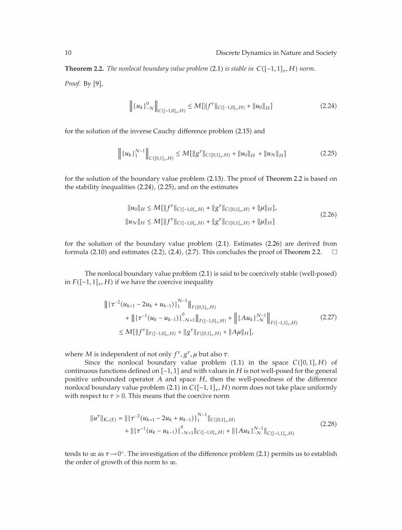
Theorem 2.2. The nonlocal boundary value problem (2.1) is stable in C([−1, 1]τ ,H) norm.

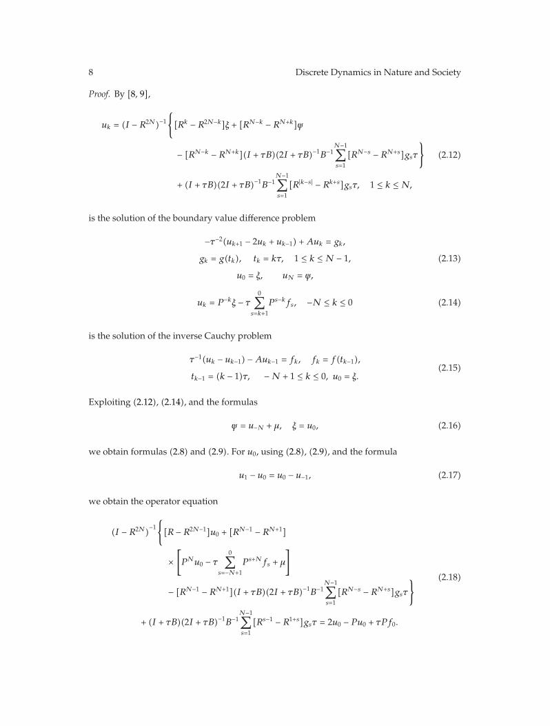
Proof. By [9],

∥∥∥{uk}0−N∥∥∥C([−1,0]τ ,H)

≤M[‖fτ‖C([−1,0]τ ,H) + ‖u0‖H] (2.24)

for the solution of the inverse Cauchy difference problem (2.15) and

∥∥∥{uk}N−11

∥∥∥C([0,1]τ ,H)

≤M[‖gτ‖C([0,1]τ ,H) + ‖u0‖H + ‖uN‖H] (2.25)

for the solution of the boundary value problem (2.13). The proof of Theorem 2.2 is based onthe stability inequalities (2.24), (2.25), and on the estimates

‖u0‖H ≤M[‖fτ‖C([−1,0]τ ,H) + ‖gτ‖C([0,1]τ ,H) + ‖μ‖H],

‖uN‖H ≤M[‖fτ‖C([−1,0]τ ,H) + ‖gτ‖C([0,1]τ ,H) + ‖μ‖H](2.26)

for the solution of the boundary value problem (2.1). Estimates (2.26) are derived fromformula (2.10) and estimates (2.2), (2.4), (2.7). This concludes the proof of Theorem 2.2.

The nonlocal boundary value problem (2.1) is said to be coercively stable (well-posed)in F([−1, 1]τ ,H) if we have the coercive inequality

∥∥{τ−2(uk+1 − 2uk + uk−1)}N−11

∥∥F([0,1]τ ,H)

+∥∥{τ−1(uk − uk−1)}0−N+1

∥∥F([−1,0]τ ,H) +

∥∥∥{Auk}N−1−N

∥∥∥F([−1,1]τ ,H)

≤M[‖fτ‖F([−1,0]τ ,H) + ‖gτ‖F([0,1]τ ,H) + ‖Aμ‖H],

(2.27)

whereM is independent of not only fτ , gτ , μ but also τ .Since the nonlocal boundary value problem (1.1) in the space C([0, 1],H) of

continuous functions defined on [−1, 1] andwith values inH is not well-posed for the generalpositive unbounded operator A and space H, then the well-posedness of the differencenonlocal boundary value problem (2.1) in C([−1, 1]τ ,H) norm does not take place uniformlywith respect to τ > 0. This means that the coercive norm

‖uτ‖Kτ (E) = ‖{τ−2(uk+1 − 2uk + uk−1)}N−11 ‖C([0,1]τ ,H)

+ ‖{τ−1(uk − uk−1)}0−N+1‖C([−1,0]τ ,H) + ‖{Auk}N−1−N ‖C([−1,1]τ ,H)

(2.28)

tends to∞ as τ→ 0+. The investigation of the difference problem (2.1) permits us to establishthe order of growth of this norm to ∞.

A. Ashyralyev and O. Gercek 11

Theorem 2.3. Assume that μ ∈ D(A) and f0 ∈ D(I + τB). Then for the solution of the differenceproblem (2.1) we have the almost coercivity inequality

‖uτ‖Kτ (E) ≤M[‖Aμ‖H + ‖(I + τB)f0‖H+min

{ln

1τ, 1 + | ln ‖A‖H→H |

}[‖fτ‖C([−1,0]τ ,H) + ‖gτ‖C([0,1]τ ,H)]],

(2.29)

whereM is independent of not only fτ , gτ , μ but also τ .

Proof. By [9],

‖{τ−1(uk − uk−1)}0−N+1‖C([−1,0]τ ,H) + ‖{Auk}0−N‖C([−1,0]τ ,H)

≤M[min

{ln

1τ, 1 + | ln ‖A‖H→H |

}‖fτ‖C([−1,0]τ ,H) + ‖Au0‖H

] (2.30)

for the solution of the inverse Cauchy difference problem (2.15) and

∥∥∥{τ−2(uk+1 − 2uk + uk−1)}N−11

∥∥∥C([0,1]τ ,H)

+∥∥∥{Auk}N−1

1

∥∥∥C([0,1]τ ,H)

≤M[min

{ln

1τ, 1 + | ln ‖A‖H→H |

}‖gτ‖C([0,1]τ ,H) + ‖Au0‖H + ‖AuN‖H

] (2.31)

for the solution of the boundary value problem (2.13). Then the proof of Theorem 2.3 is basedon the almost coercivity inequalities (2.30), (2.31), and on the estimates

‖Au0‖H ≤M[‖Aμ‖H + ‖(I + τB)f0‖H+min

{ln

1τ, 1 + | ln ‖A‖H→H |

}[‖fτ‖C([−1,0]τ ,H) + ‖gτ‖C([0,1]τ ,H)]],

‖AuN‖H ≤M[‖Aμ‖H + ‖(I + τB)f0‖H+min

{ln

1τ, 1 + | ln ‖A‖H→H |

}[‖fτ‖C([−1,0]τ ,H) + ‖gτ‖C([0,1]τ ,H)]]

(2.32)

for the solution of the boundary value problem (2.1). The proof of these estimates follows thescheme of papers [8, 9] and relies on formula (2.10) and on estimates (2.2), (2.4), and (2.7).This concludes the proof of Theorem 2.3.

Theorem 2.4. Let the assumptions of Theorem 2.3 be satisfied. Then the boundary value problem (2.1)is well-posed in a Holder space Cα

0,1([−1, 1]τ ,H) and the following coercivity inequality holds:

‖{τ−2(uk+1 − 2uk + uk−1)}N−11 ‖Cα

0,1([0,1]τ ,H)

+∥∥∥{Auk}N−1

−N∥∥∥Cα

0,1([−1,1]τ ,H)+ ‖{τ−1(uk − uk−1)}0−N+1‖Cα

0 ([−1,0]τ ,H)

≤M[‖Aμ‖H + ‖(I + τB)f0‖H +

1α(1 − α) [‖f

τ‖Cα0 ([−1,0]τ ,H) + ‖gτ‖Cα

0,1([0,1]τ ,H)]],

(2.33)

whereM is independent of not only fτ , gτ , μ but also τ and α.

12 Discrete Dynamics in Nature and Society

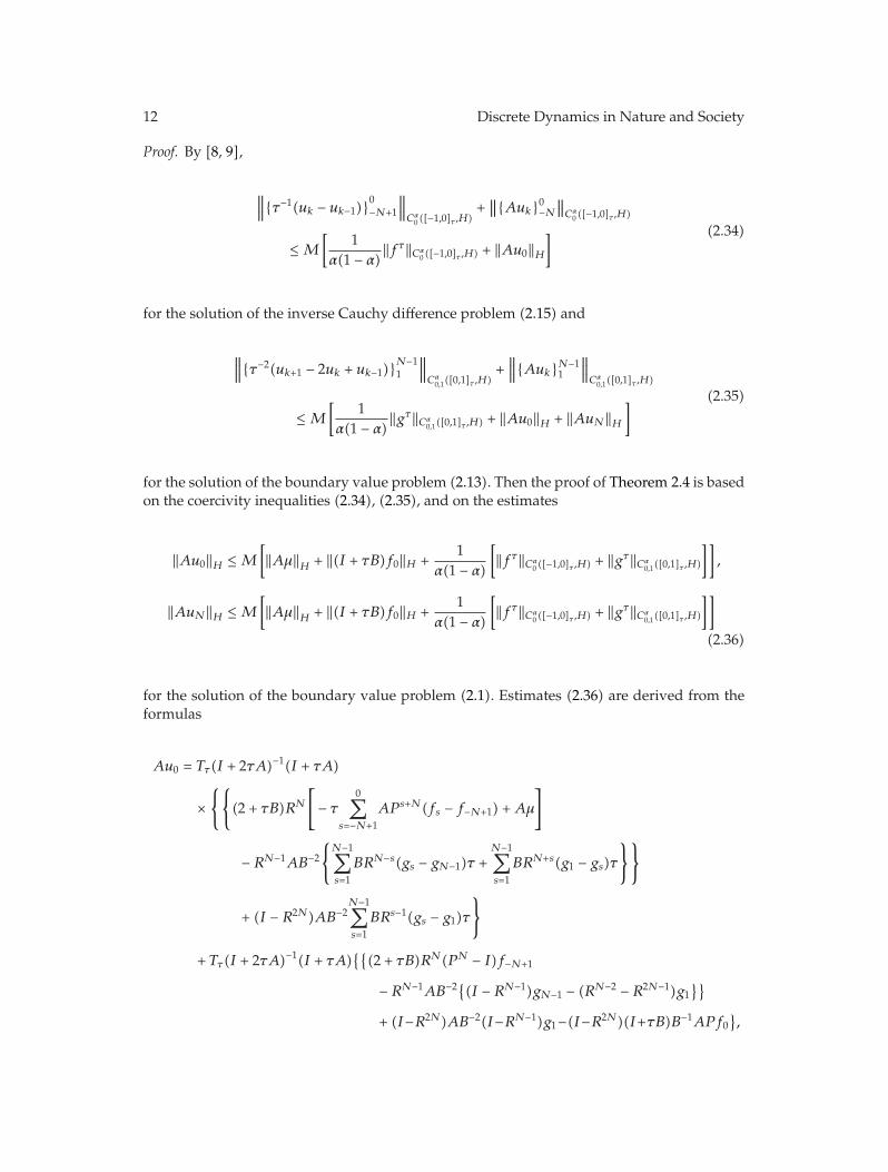
Proof. By [8, 9],

∥∥∥{τ−1(uk − uk−1)}0−N+1

∥∥∥Cα

0 ([−1,0]τ ,H)+∥∥{Auk}0−N

∥∥Cα

0 ([−1,0]τ ,H)

≤M[

1α(1 − α)‖f

τ‖Cα0 ([−1,0]τ ,H) + ‖Au0‖H

] (2.34)

for the solution of the inverse Cauchy difference problem (2.15) and

∥∥∥{τ−2(uk+1 − 2uk + uk−1)}N−11

∥∥∥Cα

0,1([0,1]τ ,H)+∥∥∥{Auk}N−1

1

∥∥∥Cα

0,1([0,1]τ ,H)

≤M[

1α(1 − α)‖g

τ‖Cα0,1([0,1]τ ,H) + ‖Au0‖H + ‖AuN‖H

] (2.35)

for the solution of the boundary value problem (2.13). Then the proof of Theorem 2.4 is basedon the coercivity inequalities (2.34), (2.35), and on the estimates

‖Au0‖H ≤M[‖Aμ‖H + ‖(I + τB)f0‖H +

1α(1 − α)

[‖fτ‖Cα

0 ([−1,0]τ ,H) + ‖gτ‖Cα0,1([0,1]τ ,H)

]],

‖AuN‖H ≤M[‖Aμ‖H + ‖(I + τB)f0‖H +

1α(1 − α)

[‖fτ‖Cα

0 ([−1,0]τ ,H) + ‖gτ‖Cα0,1([0,1]τ ,H)

]]

(2.36)

for the solution of the boundary value problem (2.1). Estimates (2.36) are derived from theformulas

Au0 = Tτ(I + 2τA)−1(I + τA)

×{{

(2 + τB)RN

[

− τ0∑

s=−N+1

APs+N(fs − f−N+1) +Aμ

]

− RN−1AB−2{N−1∑

s=1

BRN−s(gs − gN−1)τ +N−1∑

s=1

BRN+s(g1 − gs)τ}}

+ (I − R2N)AB−2N−1∑

s=1

BRs−1(gs − g1)τ}

+ Tτ(I + 2τA)−1(I + τA){{

(2 + τB)RN(PN − I)f−N+1

− RN−1AB−2{(I − RN−1)gN−1 − (RN−2 − R2N−1)g1}}

+ (I−R2N)AB−2(I−RN−1)g1−(I−R2N)(I+τB)B−1APf0},

A. Ashyralyev and O. Gercek 13

AuN = PN{

Tτ(I + 2τA)−1(I + τA)

×{{

(2 + τB)RN

[

− τ0∑

s=−N+1

APs+N(fs − f−N+1) +Aμ

]

− RN−1AB−2{N−1∑

s=1

BRN−s(gs − gN−1)τ +N−1∑

s=1

BRN+s(g1 − gs)τ}}

+ (I − R2N)AB−2N−1∑

s=1

BRs−1(gs − g1)τ}}

− τ0∑

s=−N+1

APs+N(fs − f−N+1) +Aμ + (PN − I)f−N+1

+ PN{Tτ(I + 2τA)−1(I + τA){{(2 + τB)RN(PN − I)f−N+1

− RN−1AB−2{(I − RN−1)gN−1 − (RN−2 − R2N−1)g1}}+ (I − R2N)AB−2(I − RN−1)g1 − (I − R2N)(I + τB)B−1APf0}}

(2.37)

for the solution of problem (2.1) and estimates (2.2), (2.4), and (2.7). This concludes the proofof Theorem 2.4.

Now, the applications of this abstract result to the approximate solution of themixed boundary value problem for the elliptic-parabolic equation (1.14) are considered. Thediscretization of problem (1.14) is carried out in two steps. In the first step, the grid sets

Ωh = {x = xm = (h1m1, . . . , hnmn), m = (m1, . . . , mn), 0 ≤ mr ≤Nr, hrNr = 1, r = 1, . . . , n},

Ωh = Ωh ∩Ω, Sh = Ωh ∩ S(2.38)

are defined. To the differential operator A generated by problem (1.14) we assign thedifference operator Ax

hby the formula

Axhu

hx = −

n∑

r=1

(ar(x)uhxr

)

xr ,jr(2.39)

acting in the space of grid functions uh(x), satisfying the conditions uh(x) = 0 for all x ∈ Sh.With the help of Ax

hwe arrive at the nonlocal boundary-value problem

−d2uh(t, x)dt2

+Axhu

h(t, x) = gh(t, x), 0 < t < 1, x ∈ Ωh,

duh(t, x)dt

−Axhu

h(t, x) = fh(t, x), −1 < t < 0, x ∈ Ωh,

14 Discrete Dynamics in Nature and Society

uh(−1, x) = uh(1, x) + μh(x), x ∈ Ωh,

uh(0+, x) = uh(0−, x), duh(0+, x)dt

=duh(0−, x)

dt, x ∈ Ωh

(2.40)

for an infinite system of ordinary differential equations.In the second step problem (2) is replaced by the difference scheme (2.1):

−uhk+1(x) − 2uh

k(x) + uh

k−1(x)

τ2+Ax

huhk(x) = gh

k(x),

ghk(x) = gh(tk, x), tk = kτ, 1 ≤ k ≤N − 1, Nτ = 1, x ∈ Ωh,

uhk(x) − uhk−1(x)τ

−Axhuhk−1(x) = f

hk(x),

fhk (x) = fh(tk, x), tk−1 = (k − 1)τ, −N + 1 ≤ k ≤ −1, x ∈ Ωh,

uh−N(x) = uhN(x) + μh(x), x ∈ Ωh,

uh1(x) − uh0(x) = uh0(x) − uh−1(x), x ∈ Ωh.

(2.41)

Based on the number of corollaries of the abstract theorems given above, to formulate theresult, one needs to introduce the space L2h = L2(Ωh) of all the grid functions ϕh(x) ={ϕ(h1m1, . . . , hnmn)} defined on Ωh, equipped with the norm

‖ϕh‖L2(Ωh) =

(∑

x∈Ωh

|ϕh(x)|2h1 · · ·hn)1/2

. (2.42)

Theorem 2.5. Let τ and |h| =√h21 + · · · + h2n be sufficiently small numbers. Then the solutions of

the difference scheme (2.41) satisfy the following stability and almost coercivity estimates:

∥∥∥{uhk}N−1−N

∥∥∥C([−1,1]τ ,L2h)

≤M[∥∥∥{fhk }

−1−N+1

∥∥∥C([−1,0]τ ,L2h)

+∥∥∥{ghk}

N−11

∥∥∥C([0,1]τ ,L2h)

+ ‖μh‖L2h

],

∥∥∥{τ−2

(uhk+1 − 2uhk + u

hk−1

)}N−11

∥∥∥C([0,1]τ ,L2h)

+∥∥∥{τ−1

(uhk − uhk−1

)}0−N+1

∥∥∥C([−1,0]τ ,L2h)

+∥∥∥{uhk}

N−1−N

∥∥∥C([−1,1]τ ,W2

2h)

≤M[‖μh‖W2

2h+ τ‖fh0 ‖W1

2h+ ln

1τ + |h|

[∥∥∥{fhk }−1−N+1

∥∥∥C([−1,0]τ ,L2h)

+∥∥∥{ghk}

N−11

∥∥∥C([0,1]τ ,L2h)

]],

(2.43)

whereM is independent of τ, h, μh(x), and ghk(x), 1 ≤ k ≤N − 1, fh

k,−N + 1 ≤ k ≤ 0.

A. Ashyralyev and O. Gercek 15

The proof of Theorem 2.5 is based on the abstract Theorems 2.2, 2.3, on the estimate

min{ln

1τ, 1 + | ln ‖Ax

h‖L2h →L2h |}

≤M ln1

τ + |h| (2.44)

as well as the symmetry properties of the difference operator Axhdefined by formula (2.39)

in L2h, along with the following theorem on the coercivity inequality for the solution of theelliptic difference problem in L2h.

Theorem 2.6. For the solution of the elliptic difference problem,

Axhu

h(x) = ωh(x), x ∈ Ωh, (2.45)

uh(x) = 0, x ∈ Sh, (2.46)

the following coercivity inequality holds [7]:

n∑

r=1

∥∥∥(uh)xrxr ,jr∥∥∥L2h

≤M||ωh||L2h. (2.47)

Theorem 2.7. Let τ and |h| be sufficiently small numbers. Then the solutions of the difference scheme(2.41) satisfy the following coercivity stability estimates:

∥∥∥{τ−2

(uhk+1 − 2uhk + u

hk−1

)}N−11

∥∥∥Cα

0,1([0,1]τ ,L2h)

+∥∥∥{τ−1

(uhk − uhk−1

)}0−N+1

∥∥∥Cα

0 ([−1,0]τ ,L2h)+∥∥∥{uhk}

N−1−N

∥∥∥Cα

0,1([−1,1]τ ,W22h)

≤M[‖μh‖W2

2h+ τ‖fh0 ‖W1

2h+

1α(1 − α)

[∥∥∥{fhk }−1−N+1

∥∥∥Cα

0 ([−1,0]τ ,L2h)+∥∥∥{ghk}

N−11

∥∥∥Cα

0,1([0,1]τ ,L2h)

]],

(2.48)

whereM is independent of τ, h, μh(x), and ghk (x), 1 ≤ k ≤N − 1, fhk ,−N + 1 ≤ k ≤ 0.

The proof of Theorem 2.7 is based on the abstract Theorem 2.4, the symmetryproperties of the difference operator Ax

hdefined by formula (2.39), and on Theorem 2.6 on

the coercivity inequality for the solution of the elliptic difference equation (2.45) in L2h.Note that in a similar manner the difference schemes of the first order of accuracy with

respect to one variable for approximate solutions of the boundary value problem (1.12) canbe constructed. Abstract theorems given above permit us to obtain the stability, the almoststability, and the coercive stability estimates for the solution of these difference schemes.

Acknowledgment

The authors would like to thank Professor P. E. Sobolevskii (Jerusalem, Israel) for his helpfulsuggestions to the improvement of this paper.

16 Discrete Dynamics in Nature and Society

References

[1] D. Bazarov and H. Soltanov, Some Local and Nonlocal Boundary Value Problems for Equations of Mixed andMixed-Composite Types, Ylim, Ashgabat, Turkmenistan, 1995.

[2] S. N. Glazatov, “Nonlocal boundary value problems for linear and nonlinear equations of variabletype,” Sobolev Institute of Mathematics SB RAS, no. 46, pp. 26, 1998.

[3] S. G. Krein, Linear Differential Equations in a Banach Space, Nauka, Moscow, Russia, 1967.[4] M. S. Salakhitdinov, Equations of Mixed-Composite Type, Fan, Tashkent, Uzbekistan, 1974.[5] A. Ashyralyev and H. Soltanov, “On elliptic-parabolic equations in a Hilbert space,” in Proceeding of

the IMM of CS of Turkmenistan, pp. 101–104, Ashgabat, Turkmenistan, 1995.[6] A. Ashyralyev, “A note on the nonlocal boundary value problem for elliptic-parabolic equations,”

Nonlinear Studies, vol. 13, no. 4, pp. 327–333, 2006.[7] P. E. Sobolevskiı, On Difference Methods for the Approximate Solution of Differential Equations, Voronezh

State University Press, Voronezh, Russia, 1975.[8] P. E. Sobolevskiı, “The theory of semigroups and the stability of difference schemes,” inOperator Theory

in Function Spaces (Proc. School, Novosibirsk, 1975), pp. 304–337, Nauka, Novosibirsk, Russia, 1977.[9] P. E. Sobolevskiı, “The coercive solvability of difference equations,” Doklady Akademii Nauk SSSR, vol.

201, no. 5, pp. 1063–1066, 1971.

Submit your manuscripts athttp://www.hindawi.com

Hindawi Publishing Corporationhttp://www.hindawi.com Volume 2014

MathematicsJournal of

Hindawi Publishing Corporationhttp://www.hindawi.com Volume 2014

Mathematical Problems in Engineering

Hindawi Publishing Corporationhttp://www.hindawi.com

Differential EquationsInternational Journal of

Volume 2014

Applied MathematicsJournal of

Hindawi Publishing Corporationhttp://www.hindawi.com Volume 2014

Probability and StatisticsHindawi Publishing Corporationhttp://www.hindawi.com Volume 2014

Journal of

Hindawi Publishing Corporationhttp://www.hindawi.com Volume 2014

Mathematical PhysicsAdvances in

Complex AnalysisJournal of

Hindawi Publishing Corporationhttp://www.hindawi.com Volume 2014

OptimizationJournal of

Hindawi Publishing Corporationhttp://www.hindawi.com Volume 2014

CombinatoricsHindawi Publishing Corporationhttp://www.hindawi.com Volume 2014

International Journal of

Hindawi Publishing Corporationhttp://www.hindawi.com Volume 2014

Operations ResearchAdvances in

Journal of

Hindawi Publishing Corporationhttp://www.hindawi.com Volume 2014

Function Spaces

Abstract and Applied AnalysisHindawi Publishing Corporationhttp://www.hindawi.com Volume 2014

International Journal of Mathematics and Mathematical Sciences

Hindawi Publishing Corporationhttp://www.hindawi.com Volume 2014

The Scientific World JournalHindawi Publishing Corporation http://www.hindawi.com Volume 2014

Hindawi Publishing Corporationhttp://www.hindawi.com Volume 2014

Algebra

Discrete Dynamics in Nature and Society

Hindawi Publishing Corporationhttp://www.hindawi.com Volume 2014

Hindawi Publishing Corporationhttp://www.hindawi.com Volume 2014

Decision SciencesAdvances in

Discrete MathematicsJournal of

Hindawi Publishing Corporationhttp://www.hindawi.com

Volume 2014 Hindawi Publishing Corporationhttp://www.hindawi.com Volume 2014

Stochastic AnalysisInternational Journal of