1. INTRODUCTIONThe complex electromagnetic behavior of metamaterials—artificial periodic structures with features smaller than the va-cuumwavelength—has been extensively investigated over thepast decade. An effective medium description of such struc-tures is indispensable for their analysis and design, and theexisting literature on this subject is vast. The approachesinclude retrieval via S parameters, extensions of classical mix-ing formulas for small inclusions, analysis of dipole lattices,and special current-driven models. Reviews and referencesare available in [1–3], and a recent summary can be foundin the introductions of [4,5]; see also [1–3,6–8].
The proposed homogenization theory yields an extendedsecond-order material tensor that contains not only the usual36 local material parameters, but also additional ones quanti-fying nonlocality rigorously. The local part of the tensor re-lates the mean values of the coarse-grained fields, while thenonlocal part relates these mean values to variations of thefields. This extended tensor is a key novelty of the proposedtheory and a major extension of the recently publishedmethodology [5].
Our point of departure is the traditional formulation ofMaxwell’s equations in terms of four “microscopic” fields e,d, h, and b; their coarse-grained counterparts E, D, H, andB need to be properly defined. Alternative formulations withfewer fields are available, due most notably to Landau andLifshitz [9] and Agranovich and Ginzburg [10]; see also [2].The four-field formulation, however, is universally acceptedin engineering and widely used in applied physics due to anumber of advantages. It treats intrinsic magnetism, whenit exists (at low frequencies), in a very natural way; it avoidsunnecessary nonlocality; and it yields simple local boundaryconditions without additional surface currents.
Besides, there is a certain elegance in treating two pairsof fields in a symmetric fashion [11]. If so, it is quite naturalto wonder why the same averaging procedure should not be
applied to all four microscopic fields. But, for intrinsicallynonmagnetic materials (h ¼ b), this would imply H ¼ B, lead-ing to a paradox: no magnetic effects despite the overwhelm-ing evidence to the contrary (all references on metamaterialscited above deal with magnetism in one way or another;see also [12]).
For Maxwell’s equations and standard boundary conditionsto be honored, the coarse-grained fields H and B must be ob-tained from the microscopic h and b via different procedures.Indeed, H must have tangential continuity across all inter-faces, whereas B must have normal continuity. Thisresolves the paradox arising in the four-field formulation.Specific interpolation procedures producing fields with the re-quired types of continuity are discussed in [5] and in Section 3.
The proposed theory has several distinguishing features:(i) The material is characterized by an extended parametermatrix with the usual 6 × 6 diagonal block and an off-diagonalblock that quantifies nonlocality. This generalizes the tradi-tional local treatment. (ii) The procedure is applicable to anycell size, not necessarily very small relative to the wavelength.(iii) The methodology is based on a direct field analysis in asingle lattice cell, in contrast with S-parameter retrieval pro-cedures [13–16], where the effective parameters are inferredfrom reflection and transmission coefficients of a metamater-ial slab. (iv) There are no adjustable or fitting parameters andno artificial averaging rules contrived to arrive at a desiredresult, such as magnetic permeability μ ≠ 1. Nontrivial mag-netic behavior, if present, follows logically from the method.(v) The coarse-grained fields are defined to satisfy Maxwell’sequations and interface boundary conditions exactly. (vi) Themethod can take advantage of any available (semi)analyticalor numerical approximations of the electromagnetic field in agiven lattice cell. (vii) The approximations made and the re-spective errors are clearly and explicitly identified and quan-tified not only in the asymptotic “big-O” sense but numericallyas well. (viii) The model of nonlocality resulting from the
2956 J. Opt. Soc. Am. B / Vol. 28, No. 12 / December 2011 Igor Tsukerman
theory can be incorporated into existing methods and soft-ware for field simulation. However, this subject is beyondthe scope of the present paper and will be analyzed elsewhere.(ix) The theory is minimalistic, with only a few fundamentalpremises at its core; see Section 2.
Of a very large number of homogenization methods in theexisting literature, two need to be mentioned separately: onedue to its very wide acceptance and the other one due to itsspecial relevance to the present paper. In one most commonprocedure, effective parameters of a metamaterial slab are“retrieved” from transmission/reflection data (i.e., from theS parameters) [13–16]. Being essentially an inverse problem,this parameter retrieval has some inherent ill-posedness thatmanifests itself in the multiplicity of solutions, due to the am-biguity of branches of the inverse trigonometric functions in-volved. Parameters retrieved for slabs of varying thickness(let alone shape) are not always consistent. More fundamen-tally, the retrieval procedure does not by itself explain whysuch consistency should be expected; obviously, there mustbe an underlying reason for it. That deeper reason is the de-finition of material parameters as relations between the (pairsof) coarse-grained fields.
The existing approach most closely related to the metho-dology of the present paper is due to the insight of Smithand Pendry, who suggested different averaging proceduresfor different fields in the cell [7]. This idea, subsequently ela-borated in [17], stemmed from the analogy with finite differ-ence schemes on staggered grids. The present paper, alongwith [5], provides an expanded and substantially more rigor-ous foundation for this physical insight, as well as a muchmore comprehensive description of the behavior of the fieldsin terms of the extended material tensor comprising local andnonlocal parameters. The exposition below starts with a gen-eral description of the key concepts, followed by some tech-nical details, implementation and examples.
2. PROPOSED THEORY: KEY CONCEPTSSince material parameters are linear relations between thecoarse-grained fields, a natural plan is to define these fieldsclearly and then establish a linear mapping between the ðH;EÞand ðB;DÞ pairs. The motivation for any effective medium the-ory is that the microscopic fields vary too rapidly to be easilydescribed and analyzed; one may say that they have “too manydegrees of freedom” (DOF). An obvious idea is to split thefields up into coarse-grained (capital letters) and fast (tildeletters) components; e.g., b ¼ Bþ b∼. For reasons articulatedbelow, this splitting should satisfy several conditions:
1. By definition, the coarse-grained fields must vary muchless rapidly than the total fields. Nevertheless, the formermust approximate the latter, in a certain well-defined sense,everywhere in space.
2. The coarse-grained fields must satisfy Maxwell’s equa-tions and interface boundary conditions.
3. The fast and coarse components must be semide-coupled. That is, the fast components may depend on thecoarse ones, but the coarse fields must not depend, or maydepend only very weakly, on the fast ones.
4. There exists a linear relation (map) between the pairs ofcoarse-grained fields ðE;HÞ and ðD;BÞ that is independent ofthe incident waves (at least to a given level of approximation).
The requirements above define not a single method but aframework from which conceptually similar but not fullyequivalent homogenization methods could be obtained bymaking these requirements more specific.
The rationale for each of the conditions above is as follows.The first one represents, from the physical perspective, thevery essence of homogenization. From a more mathematicalviewpoint of analysis and simulation, one might accept aweaker requirement that the coarse fields could be describedwith much fewer DOF but would not necessarily have to varyless rapidly than the total fields. For example, the field in aperiodic structure can in many cases be described by a verylimited number of Bloch waves with judiciously chosen wavevectors (see, e.g., [18] for some illuminating examples); thisfact may be effectively used in semianalytical and numericalmethods, such as the generalized finite element method[19–21], discontinuous Galerkin methods [22], and flexible lo-cal approximation methods (FLAME) [23–25]. Nevertheless,the focus of this paper is on physical, not numerical, methods.
Pointwise approximation of the microscopic fields by thecoarse ones is in general not feasible and not required, as ra-pid local field oscillations due to the resonance effects in me-tamaterial cells are definitely of interest. Instead, we assumethat the coarse-grained fields are close to the real ones at thecell boundary, where the fields vary more smoothly. Inside thecell, the coarse-grained fields are defined by interpolationfrom the boundary values.
Although the second requirement (coarse-grained fieldssatisfying Maxwell’s equations) seems to be self-evident, manyexisting methods pay surprisingly little attention to it and mayactually violate it. In particular, coarse fields defined viasimple volume averaging do not satisfy Maxwell’s boundaryconditions. We shall return to this important point later.
The rationale for the third requirement (weak coupling)is that, if both components were to be coupled strongly, thetwo-scale problem would not be any simpler than the originalone involving the total field.
The fourth requirement is, for now, open ended and needsto be made more specific. Let us assume that, for a given mi-croscopic field ðe;d;bÞ, the coarse-grained fields ðE;D;B;HÞsatisfying conditions 1–3 above have been defined in someway. The central question then is to relate the pairs ofcoarse-grained fields. The generalized “material parameter” is,mathematically, a linear map L:ðE;HÞ → ðD;BÞ from the func-tional space of fields ðE;HÞ to the functional space of ðD;BÞ.The dimensionality of this map depends on the coarse-grainedinterpolations chosen. A high-dimensional linear map couldbe of use in numerical procedures but does not offer muchphysical insight. One critical question then is whether a goodlow-dimensional approximation of this linear map can befound. A formal linear-algebraic answer to this question is wellknown: the best approximation of a given rectangular matrixby a matrix of rank m is via the highest m singular values andthe respective singular vectors (see, e.g., [26] or [27] for themathematical details). The error of this approximation isequal to the mþ 1st singular value. One may note a concep-tual similarity with the well-known principal component ana-lysis (PCA); see, e.g., [28] for an elementary tutorial.
Although the PCA analogy is instructive, it does not providea direct connection with the physical parameters such as ε orμ. Our objective is still to find new bases in which the material
Igor Tsukerman Vol. 28, No. 12 / December 2011 / J. Opt. Soc. Am. B 2957
map L could be “compressed” to a low-dimensional form, butthe bases we are seeking are physical rather than formally al-gebraic. More specifically, in this physical basis the first fewcomponents of the coarse-grained fields E, H, D, B are to betheir mean values, and the subsequent components—the de-viations from the mean. Such bases and the respective matrixrepresentation of the map L will be called canonical and aredescribed in Section 3 in detail.
3. PROPOSED THEORY: DETAILSA. EquationsConsider a periodic structure composed of materials thatare assumed to be (i) intrinsically nonmagnetic (which is trueat sufficiently high frequencies [9]) and (ii) satisfy a linearlocal constitutive relation d ¼ εe. For simplicity, we assumea cubic lattice with cells of size a. Maxwell’s equations forthe microscopic fields are, in the frequency domain and withthe expð−iωtÞ phasor convention, ∇ × e ¼ iωc−1b, ∇ × b ¼−iωc−1d. As in [5], small letters b, e, d, etc., denote the “micro-scopic”—i.e., true physical—fields that in general vary rapidlyin space (but still on the scale ⪆10nm, so that the intrinsicpermittivity is physically meaningful). Capital letters referto smoother fields that vary on the scale coarser than the lat-tice cell size. These coarse-grained fields B, H, E, and D mustbe defined in such a way that the boundary conditions are ho-nored. Simple cell averaging does not satisfy this condition [5].To understand why, consider, say, the “microscopic”magneticfield, for simplicity just a function of one coordinate, bðxÞ, at amaterial/air interface x ¼ 0. For intrinsically nonmagneticmedia, this field is continuous across the interface; i.e.,bð0−Þ ¼ bð0þÞ. Since the field fluctuates in the material, thereis no reason for its value at x ¼ 0þ to be equal to its cell aver-age over 0 ≤ x ≤ a, except by coincidence. Thus, if this cellaverage is used to define the B field, its normal componentat the interface will almost always be discontinuous, whichis nonphysical. As a rough, “zero-order,” approximation, thesenonphysical field jumps across the interface could be ne-glected. This may indeed be possible in the absence of reso-nances or for vanishingly small cell sizes. However, neglecting
strong field fluctuations in other cases would eliminate thevery resonance effects that we wish to capture.
The general stages of the method are shown in Fig. 1. Thefield in the lattice cell is approximated with a superposition ofseveral modes (e.g., Bloch waves in the periodic case). Eachof these modes is then “coarse grained” by two complemen-tary interpolation procedures, div-conforming for the ðD;BÞfields and curl-conforming for ðE;HÞ (Subsection 3.B). The ex-tended material tensor is then found as a linear map betweenthese field pairs.
B. Coarse-Grained Fields: Interpolation and ContinuityConditionsThis is a key point, where we depart from more traditionalmethods of field averaging. The coarse-grained E and H fieldsare produced from the “microscopic” ones, e and b, by an in-terpolation that respects tangential continuity across all inter-faces. The coarse-grained D and B fields are produced from dand b by another interpolation, one that preserves normalcontinuity.
Tangentially continuous interpolation is effected by vector-ial functions like the one shown in Fig. 2, in a 2D rendition forsimplicity. The circulation of this function is equal to onealong one edge (in the figure, the vertical edge shared by twoadjacent lattice cells) and zero along all other edges of thelattice. To shorten all interpolation-related expressions, inthis section, the lattice cell is normalized to the unit cube
½0; 1�3; i.e., a ¼ 1. Then a formal expression for four x-directedfunctions w is w1−4 ¼ xfyz; ð1 − yÞz; yð1 − zÞ; ð1 − yÞð1 − zÞg.Another eight functions of this kind are obtained by the cyclicpermutation of coordinates in the expression above. For eachlattice cell, there are 12 such interpolating functions alto-gether (one per edge). Each function wα has unit circulationalong edge αðα ¼ 1; 2;…12Þ and zero circulations along allother edges. All of them are vectorial interpolating functions,bilinear with respect to the spatial coordinates. (In [5] thesefunctions were defined in the cell scaled to ½−1; 1�3 rather thanto ½0; 1�3, and therefore the algebraic expressions differ.)
The coarse-grained E and H fields can then be representedby interpolation from the edges into the volume of the cell asfollows:
Fig. 1. (Color online) Key parts of the proposed methodology.Two types of interpolation are used to obtain the coarse-grained fieldswith tangential and normal continuity. The electromagnetic field in-side the cell, with all its microstructure, is approximated as a super-position of basis modes. Material parameters are linear relationshipsbetween the pairs of coarse-grained fields.
Fig. 2. (Color online) (From [5].) 2D analog of the vectorial interpo-lation function wα (in this case, associated with the central verticaledge shared by two adjacent cells). The tangential continuity of thisfunction is evident from the arrow plot; its circulation is equal to oneover the central edge and to zero over all other edges.
2958 J. Opt. Soc. Am. B / Vol. 28, No. 12 / December 2011 Igor Tsukerman
E ¼X12
α¼1
½e�αwα; H ¼X12
α¼1
½b�αwα; ð1Þ
where ½e�α ¼Rα e · dl is the circulation of the (microscopic) e
field along edge α, similarly for ½b�α. In the calculation of thecirculations, integration along the edge is always assumed tobe in the positive direction of the respective coordinate axis.
Now consider the second kind of interpolation that pre-serves the normal continuity and produces the D, B fieldsfrom d and b. A typical interpolating function (a 2D rendition,again for simplicity) is shown in Fig. 3. The flux of this func-tion through a face shared by two adjacent cells is equal toone; the flux through all other faces is zero. Two such func-tions in the x direction are (as before, for the cell size normal-ized to unity) v1−2 ¼ xfx; 1 − xg, and another four functionsv3−6, in the y and z directions, are expressed similarly. Thesesix functions can be used to define the coarse-grainedD and Bfields by interpolation from the six faces into the volume ofthe unit cell:
D ¼X6
β¼1
½½d��βvβ; B ¼X6
β¼1
½½b��βvβ; ð2Þ
where ½½d��β ¼Rβ d · dS is the flux of d through face
βðβ ¼ 1; 2;…; 6Þ; similarly for the b field. In the calculation offluxes, it is convenient to take the normal to any face in thepositive direction of the respective coordinate axis (ratherthan in the outward direction).
The coarse-grained E and H fields so defined have 12 DOFin any given lattice cell—mathematically, they lie in the12-dimensional functional space spanned by functions wα.This space was denoted withWcurl in [5]: the “W” honors Whit-ney [29], and “curl” indicates fields whose curl is a regularfunction rather than a general distribution. This implies, inphysical terms, the absence of equivalent surface currents andthe tangential continuity of the fields involved.
Similarly, D and B within any lattice cell lie in the six-dimensional functional space Wdiv spanned by functions vβ.Importantly, it can be shown that the div and curl spaces arecompatible in the following sense:
∇ ×Wcurl⊂Wdiv: ð3Þ
That is, the curl of any function fromWcurl [i.e., the curl of anycoarse-grained field E or H Eq. (1)] lies in Wdiv. Because of
this compatibility of interpolations, the coarse-grained fieldssatisfy Maxwell’s equations exactly [5]:
∇ × E ¼ iωc−1B; ∇ ×H ¼ −iωc−1D: ð4Þ
By construction, they also satisfy the proper continuityconditions at all interfaces.
To recap the ideas, Fig. 4 schematically illustrates the inter-polation procedures and the linear-algebraic part of the pro-posed method. The simplified 1D rendition shows only the xaxis, the tangential (y; z) components of E, H, and the normal(x) component of D, B. Other components (not shown) maybe discontinuous at cell boundaries and at material interfaces.The linear operator L relating the pairs of coarse-grainedfields is, in general, multidimensional, commensurate withthe dimensions of the interpolation spaces chosen. As we shallsee, L has a 6 × 6 (or smaller) matrix block in a suitable “ca-nonical” basis; this block relates the field averages of ðD;BÞ tothe field averages of ðE;HÞ. The remainder of the matrix re-lates the field averages to field variations over the cell andcan be viewed as a manifestation of nonlocality (see Section 4for further details).
C. Approximating FunctionsThe actual microscopic fields in the material are not fixedand not known; they need to be approximated by introducingsuitable basis functions (BFs) [5]. Examples include Blochwaves in the periodic case, plane waves, and spherical harmo-nics. For a nonvanishing cell size, the field has an infinitenumber of DOF; thus, as a matter of principle, its representa-tion in a finite basis is approximate. Nevertheless, the relevantbehavior of the fields can be captured very well by relativelysmall bases [18]. By expanding the bases, one can representthe fieldsmore accurately, at the expenseof higher complexity.A small number of BF corresponds to local material para-meters, a moderately higher number—to nonlocal ones, anda large number falls under the umbrella of numerical simula-tion. This viewpoint unifies local, nonlocal, and numerical
treatment of electromagnetic characteristics ofmetamaterials.In the periodic case, the most natural basis modes are
Bloch waves traveling in different directions (the approxima-tion accuracy for the field in general depends on the number
Fig. 3. (Color online) (From [5].) 2D analog of the vectorial interpo-lation function vβ (in this case, associated with the central verticaledge). The normal continuity of this function is evident from the arrowplot; its flux is equal to one over the central edge and zero over allother edges. Fig. 4. (Color online) Linear relation between the coarse-grained
fields. E, H are interpolated to ensure tangential continuity; D, Bare normally continuous (1D rendition for simplicity). Operator Lis, in general, multidimensional. In a canonical basis, L contains a6 × 6 submatrix of local electrodynamic parameters.
Igor Tsukerman Vol. 28, No. 12 / December 2011 / J. Opt. Soc. Am. B 2959
of basis modes chosen). If the structure is not necessarily per-iodic, one may note that tangential components of the electricor, alternatively, magnetic field on the cell boundary definethe field inside the cell uniquely, except for the special casesof interior resonances. To specify the basis, it is thus sufficientto consider the boundary values in lieu of the values inside ofthe cell. A natural set of approximating functions can thus beobtained by setting the tangential components of E or H onthe cell boundary as low-order polynomials and using thatas Dirichlet conditions for Maxwell’s equations within thecell. This alternative to Bloch modes will be explored in moredetail in the future.
More formally, let the electromagnetic field be approxi-mated as a linear combination of some basis waves (modes)ψα [5]:
Ψeh ¼X
αcαψeh
α þ δeh; Ψdb ¼X
αcαψdb
α þ δdb: ð5Þ
In general,Ψ and all ψα are six-component vectors comprisingboth microscopic fields; e.g., Ψeh ≡ fΨe;Ψhg, etc. The δs areapproximation errors that will tend to decrease as moremodes are included in the expansion.
D. Canonical BasisBy construction of the coarse-grained interpolants, the Eand H fields, taken together within a lattice cell, lie in a 24-dimensional linear space (12 edge-based DOF for each field),while the D and B fields together lie in a 12-dimensional space(six face-based DOF for each field). Therefore, a linear rela-tionship between these pairs of fields is, technically, a mapfrom a complex 24-dimensional space to a 12-dimensionalone. For a given pair of bases in these spaces, this map is de-scribed by a 24 × 12 complex matrix and can be viewed as ageneralized material tensor. However, there is one importantcaveat and a necessary amendment.
The caveat is that there exist linear relationships betweenthe above-mentioned DOF that follow directly from Maxwell’sequations, regardless of the content of the lattice cell. For ex-ample, Faraday’s law relates the edge circulations of the elec-tric field over any face of the cell and the magnetic fluxthrough the same face. Such Maxwell dependencies needto be eliminated before the generalized material tensor issought. This could be done in a formal linear-algebraic way;however, to stay closely connected with physical parameters,let us define a natural, “canonical,” set of DOF as follows.
Boundary averages of the coarse fields, i.e., hE × ni∂Ω,hH × ni∂Ω, hnðD · nÞi∂Ω, hnðB · nÞi∂Ω. To reiterate, it is the tan-gential components of E, H and the normal componentsof D, B that are being averaged. The coarse-grained fieldsinside the cell are produced by low-order Whitney-like inter-polation of the boundary values, and it is easier to use bound-ary averages of these fields as a proxy for their volumeaverages. There are six DOF in this category altogetherfor the ðE;HÞ pair (three Cartesian components for each meanfield) and six DOF for the ðD;BÞ pair.
Boundary averages of a subset of first partial deriva-tives of ðE;HÞ: h∂Ex=∂yi∂Ω, h∂Ey=∂zi∂Ω, h∂Ez=∂xi∂Ω, andsimilarly for H.
Boundary averages of a subset of second partialderivatives of ðE;HÞ.
Several comments are in order with regard to this choice ofDOF (i) We are generally interested in expressing the meanvalues of ðD;BÞ, but not their derivatives, in terms of ðE;HÞand (if necessary) of the variations of ðE;HÞ within the cell.Hence the derivatives of ðE;HÞ are included into considera-tion, while those of ðD;BÞ do not have to be. (ii) The DOF can-not simultaneously contain, say, h∂Ex=∂yi∂Ω and h∂Ey=∂xi∂Ω,because their difference constitutes h∇ × Eiz and is directlyrelated to Bz via Faraday’s law regardless of the content ofthe lattice cell. However, it is possible to use linear combina-tions independent of the curl and symmetrize the derivatives:h∂Ex=∂yþ ∂Ey=∂xi∂Ω, etc. (iii) Considerations regarding thesecond derivatives are similar but more involved. In particu-lar, the Laplacian of the field on the cell boundary is related,via the wave equation, to the field itself. Thus, including allsecond derivatives in the set of DOF may be redundant. (iv) Itis clear from the above that the choice of the additional “non-local” DOF is not unique. Different choices will lead to meth-ods that are conceptually similar but differ in the particularways of quantifying nonlocality. Thus we have a spectrumof methods—a framework—rather than a single method.(v) Some DOF may vanish due to symmetry. For example,if the lattice cell is symmetric with respect to x, the x deriva-tives of the fields need not be included.
E. Generalized Material TensorWe are now in a position to describe the algorithmic stages forobtaining the generalized material tensor:
1. Choose a set of N approximating modes, and computethese modes using any analytical, semianalytical, or numericaltools available.
2. Choose a set of MEH and MDB DOF for the ðE;HÞ andðD;BÞ pairs, respectively, as described in the previous subsec-tion. The DOF will, in general, include the mean values of thetangential components of E, H and of the normal componentsof D, B; in addition, the mean values of some derivativesof E, H may be included. By increasing the number of DOF,one trades higher accuracy for a greater level of nonlocality inthe characterization of the material. Typically for 3D pro-blems,MDB ¼ 6 (three mean values for each of the two fields)butMEH ≥ 6 (nonlocal DOF may be included in addition to themean values).
3. For each mode m ¼ 1; 2;…M , compute its respectiveDOF (the mean boundary values of the tangential componentsof E, H for this mode, etc.) Assemble the DOF for the E, Hfields into the mth column of matrix WEH and the DOF forthe D, B fields into themth column of matrixWDB. Ultimately,matrix WEH is of dimension MEH × N and matrix WDB isMDB × N (typically 3 × N).
4. Find the extended material tensor η as a solution of (ingeneral) the least-squares problem
ηWEH ¼l:s: WDB ⇒ η ¼ WDBWEHþ; ð6Þ
where “þ” indicates the Moore–Penrose pseudoinverse [26].In contrast with the procedure of [5], the matrices in Eq. (6)are not position dependent. Another beneficial difference with[5] is that the pseudoinverse turns into a regular inverse ifWEH is a square matrix, i.e., if the number of DOF MEH isequal to the number of basis modes N .
2960 J. Opt. Soc. Am. B / Vol. 28, No. 12 / December 2011 Igor Tsukerman
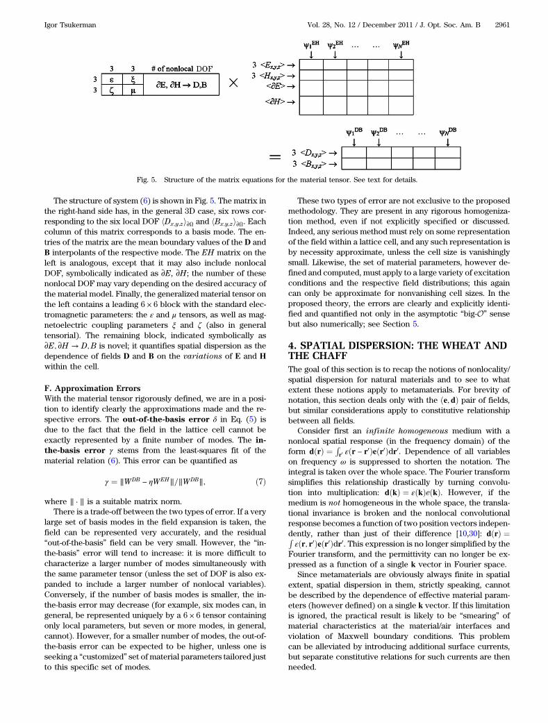
The structure of system (6) is shown in Fig. 5. The matrix inthe right-hand side has, in the general 3D case, six rows cor-responding to the six local DOF hDx;y;zi∂Ω and hBx;y;zi∂Ω. Eachcolumn of this matrix corresponds to a basis mode. The en-tries of the matrix are the mean boundary values of the D andB interpolants of the respective mode. The EH matrix on theleft is analogous, except that it may also include nonlocalDOF, symbolically indicated as ∂E, ∂H; the number of thesenonlocal DOF may vary depending on the desired accuracy ofthe material model. Finally, the generalized material tensor onthe left contains a leading 6 × 6 block with the standard elec-tromagnetic parameters: the ε and μ tensors, as well as mag-netoelectric coupling parameters ξ and ζ (also in generaltensorial). The remaining block, indicated symbolically as∂E; ∂H → D;B is novel; it quantifies spatial dispersion as thedependence of fields D and B on the variations of E and Hwithin the cell.
F. Approximation ErrorsWith the material tensor rigorously defined, we are in a posi-tion to identify clearly the approximations made and the re-spective errors. The out-of-the-basis error δ in Eq. (5) isdue to the fact that the field in the lattice cell cannot beexactly represented by a finite number of modes. The in-the-basis error γ stems from the least-squares fit of thematerial relation (6). This error can be quantified as
γ ¼ ∥WDB − ηWEH∥=∥WDB∥; ð7Þ
where ∥ · ∥ is a suitable matrix norm.There is a trade-off between the two types of error. If a very
large set of basis modes in the field expansion is taken, thefield can be represented very accurately, and the residual“out-of-the-basis” field can be very small. However, the “in-the-basis” error will tend to increase: it is more difficult tocharacterize a larger number of modes simultaneously withthe same parameter tensor (unless the set of DOF is also ex-panded to include a larger number of nonlocal variables).Conversely, if the number of basis modes is smaller, the in-the-basis error may decrease (for example, six modes can, ingeneral, be represented uniquely by a 6 × 6 tensor containingonly local parameters, but seven or more modes, in general,cannot). However, for a smaller number of modes, the out-of-the-basis error can be expected to be higher, unless one isseeking a “customized” set of material parameters tailored justto this specific set of modes.
These two types of error are not exclusive to the proposedmethodology. They are present in any rigorous homogeniza-tion method, even if not explicitly specified or discussed.Indeed, any serious method must rely on some representationof the field within a lattice cell, and any such representation isby necessity approximate, unless the cell size is vanishinglysmall. Likewise, the set of material parameters, however de-fined and computed, must apply to a large variety of excitationconditions and the respective field distributions; this againcan only be approximate for nonvanishing cell sizes. In theproposed theory, the errors are clearly and explicitly identi-fied and quantified not only in the asymptotic “big-O” sensebut also numerically; see Section 5.
4. SPATIAL DISPERSION: THE WHEAT ANDTHE CHAFFThe goal of this section is to recap the notions of nonlocality/spatial dispersion for natural materials and to see to whatextent these notions apply to metamaterials. For brevity ofnotation, this section deals only with the ðe;dÞ pair of fields,but similar considerations apply to constitutive relationshipbetween all fields.
Consider first an infinite homogeneous medium with anonlocal spatial response (in the frequency domain) of theform dðrÞ ¼ R
r0 εðr − r0Þeðr0Þdr0. Dependence of all variableson frequency ω is suppressed to shorten the notation. Theintegral is taken over the whole space. The Fourier transformsimplifies this relationship drastically by turning convolu-tion into multiplication: dðkÞ ¼ εðkÞeðkÞ. However, if themedium is not homogeneous in the whole space, the transla-tional invariance is broken and the nonlocal convolutionalresponse becomes a function of two position vectors indepen-dently, rather than just of their difference [10,30]: dðrÞ ¼Rεðr; r0Þeðr0Þdr0. This expression is no longer simplified by the
Fourier transform, and the permittivity can no longer be ex-pressed as a function of a single k vector in Fourier space.
Since metamaterials are obviously always finite in spatialextent, spatial dispersion in them, strictly speaking, cannotbe described by the dependence of effective material param-eters (however defined) on a single k vector. If this limitationis ignored, the practical result is likely to be “smearing” ofmaterial characteristics at the material/air interfaces andviolation of Maxwell boundary conditions. This problemcan be alleviated by introducing additional surface currents,but separate constitutive relations for such currents are thenneeded.
Fig. 5. Structure of the matrix equations for the material tensor. See text for details.
Igor Tsukerman Vol. 28, No. 12 / December 2011 / J. Opt. Soc. Am. B 2961
Still, in many publications, material parameters are derivedfor a single wave—either a Bloch wave or a wave generated bysome special auxiliary sources [4,6,8]—and then dependenceof these parameters on the wave vector k is investigated. Thisapproach raises further questions, in addition to the lack oftranslational invariance noted above. First, fundamentally,electromagnetic parameters cannot be defined only fromwaves propagating in the bulk [5]. This is so because a gaugingtransformation may change the relationships between thefields while leaving Maxwell’s equations unchanged [5,31].It is through the boundary conditions on the material/air(or material/dielectric) interfaces that the d and h fields aregauged uniquely.
Second, a natural definition of material parameters for asingle Bloch wave propagating in the bulk of an intrinsicallynonmagnetic metamaterial yields only a trivial result forthe effective magnetic permeability, and hence artificialmagnetism cannot be explained. To elaborate, consider anx-polarized Bloch wave traveling in the z direction (e.g.,[24,32]):
eBðzÞ ¼ EPERðzÞ expðiKBzÞxiωc−1bBðzÞ ¼ yðE0
PERðzÞ þ iKBEPERðzÞÞ expðiKBzÞ: ð8Þ
Here “PER” indicates a cell-periodic factor and KB is theBloch wavenumber. For this Bloch wave to mimic a planewave in an equivalent effective medium, the dispersion rela-tion and the wave impedance must be
ω2μeffεeff ¼ K2B; ð9Þ
ðμeff=εeffÞ12 ¼ heBi=hbBi ¼ ω=KB: ð10Þ
Cell averaging h·i eliminates E0PER and leaves only the dc
component in EPER. From the two conditions above, it followsimmediately that μeff ¼ 1.
Third, even if all the complications above are somehowcircumvented, a single Bloch or plane wave still does not carryenough information identifying the whole 6 × 6 materialparameter matrix, so the problem is badly underdetermined.Recognizing that, Fietz and Shvets [4] consider a collection oftest waves that allows one to set up a system of equationsfor all parameters. A critique of these approaches can be
found in [33] but is not directly relevant in the context ofthe present paper.
All of this is not to say that “spatial dispersion” is an invalidnotion for metamaterials. To the contrary, the theory pro-posed in this paper does lead to its precise andmathematicallyquantifiable definition. The message here is that “spatial dis-persion” is a loaded expression that should be used with ex-treme care and with accurate definitions; it cannot be blindlytransplanted from the analysis of natural materials to metama-terials. For natural media, the material parameters are extra-
neous to the Maxwell model (they come from measurementssupported by theoretical considerations), so a reasonableparticular form of k dependence can just be postulated.In contrast, the Maxwell model for metamaterials (with givenintrinsic characteristics of all natural components involved) iscompletely self-contained and does not include any extra-neous parameters. “Spatial dispersion” in metamaterials re-mains a heuristic notion or even a figure of speech unless anduntil the effective parameters are clearly and rigorously
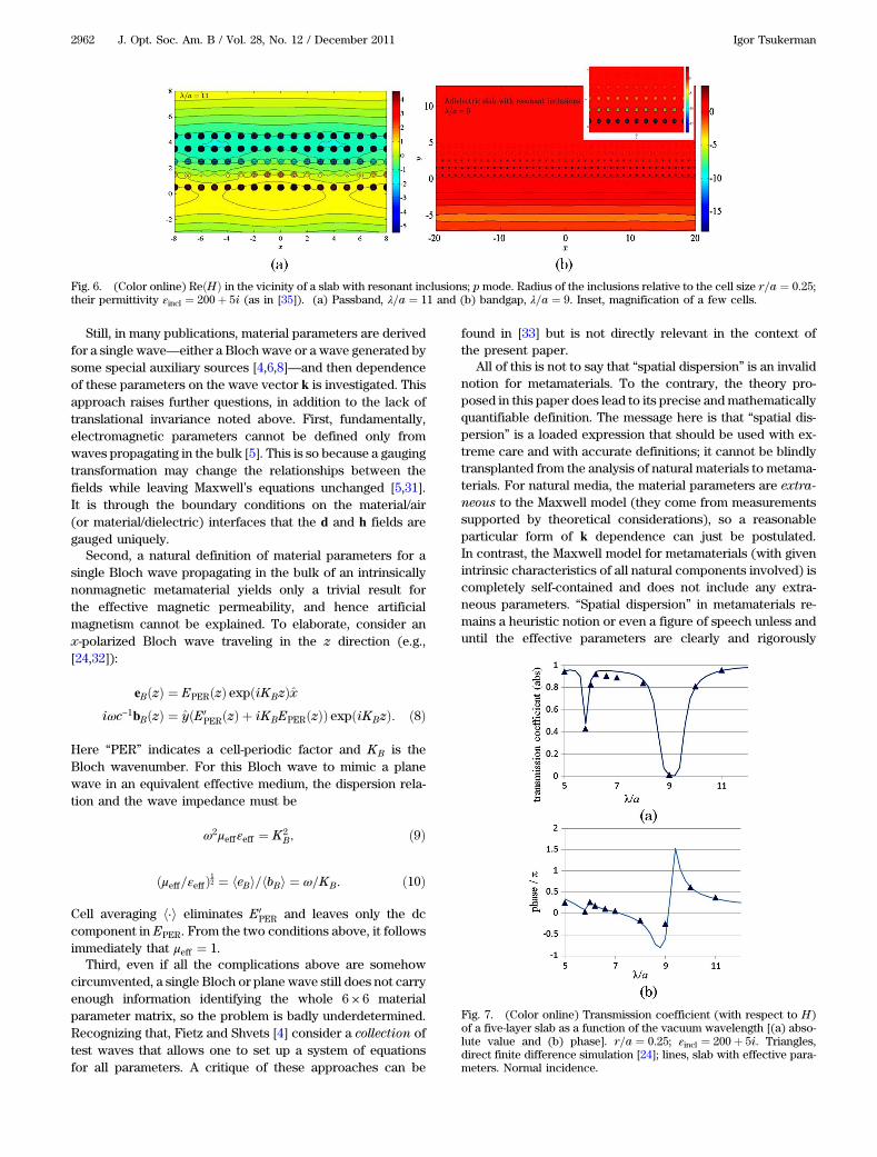
Fig. 6. (Color online) ReðHÞ in the vicinity of a slab with resonant inclusions; pmode. Radius of the inclusions relative to the cell size r=a ¼ 0:25;their permittivity εincl ¼ 200þ 5i (as in [35]). (a) Passband, λ=a ¼ 11 and (b) bandgap, λ=a ¼ 9. Inset, magnification of a few cells.
Fig. 7. (Color online) Transmission coefficient (with respect to H)of a five-layer slab as a function of the vacuum wavelength [(a) abso-lute value and (b) phase]. r=a ¼ 0:25; εincl ¼ 200þ 5i. Triangles,direct finite difference simulation [24]; lines, slab with effective para-meters. Normal incidence.
2962 J. Opt. Soc. Am. B / Vol. 28, No. 12 / December 2011 Igor Tsukerman
defined. This, in turn, requires a precise definition of thecoarse-grained fields.
5. APPLICATION EXAMPLES
A. Single Inclusion with Interior ResonancesThis example involves high-permittivity inclusions withstrong resonance effects. The setup and parameters are verysimilar to the ones in [34,35], where a special asymptoticmethod was developed and additional adjustable parameterswere needed [35]. The methodology of the present paperhandles this case with ease and without any additional as-sumptions or parameters.
The lattice cell contains a high-permittivity cylindrical in-clusion (εincl ¼ 200þ 5i); its radius relative to the cell size
is r=a ¼ 0:25; the normalized vacuum wavelength λ=a variesfrom 5 to 12. Most interesting is the H mode (p mode), wherethe electric field cuts across the cylinders and strong reso-nances can be induced.
The effective medium theory developed here agrees verywell with “brute force” finite difference simulations, whereall inclusions are represented directly. As in [5], the propaga-tion of waves through a homogeneous “effective parameter”slab is compared with the numerical simulation of this propa-gation through the actual metamaterial. Highly accurate finitedifference “FLAME” schemes [23–25] were used for the nu-merical simulation. Figure 6 illustrates the distribution ofthe real part of the magnetic field for normal incidence in thepassband, λ=a ¼ 11, and in the bandgap, λ=a ¼ 9. Figure 7demonstrates that the transmission coefficient for the slabwith effective parameters is very close, both in the absolutevalue and phase, to the “true” coefficient from the FLAME si-mulation. The effective parameters plotted in Fig. 8 exhibit anelectric resonance near λ=a ∼ 5:5 and a strong magnetic reso-nance around λ=a ∼ 9. As should be expected by symmetryconsiderations, the magnetoelectric coupling in this exampleis zero (numerically, it is at the round-off error level). The in-the-basis error γ Eq. (7) is below 10% for λ=a ⪆ 5 and under 5%for λ=a ⪆ 9, as shown in Fig. 9.
B. Particle Trimer with Interior ResonancesA second example involves a trimer of nanoparticles with thesame high value of the dielectric permittivity as before,ε ¼ 200þ 5i, but with a twice smaller radius r=a ¼ 0:125.The H mode (p polarization) is again of greater interestdue to the interior resonances in the trimer. The particlesare centered at points ð−0:05;−0:2Þ, ð0:2; 0:15Þ, ð−0:2; 0:175Þwithin the lattice cell normalized to unit size. The basis modesare eight Bloch waves traveling in the directions ϕm ¼ mπ=4(m ¼ 0; 1;…; 7) relative to the x axis. Two such modes, forλ=a ¼ 4:6 and 8, with αm ¼ π=4 are displayed in Fig. 10 asan example.
The choice of the nonlocal DOF for H comes from the fol-lowing considerations. The x and y derivatives of H are pro-portional to Dy and Dx and hence (on the boundary) to Ey andEx, respectively. These DOF would therefore be redundantbecause the electric field is already included in the local
Fig. 8. (Color online) Effective parameters of the metamaterial withresonant inclusions.
Fig. 9. (Color online) In-the-basis error γ for the metamaterial withresonant inclusions.
Fig. 10. (Color online) Examples of Bloch modes in a nanoparticle trimer. r=a ¼ 0:125; εincl ¼ 200þ 5i for all three particles. (a) λ=a ¼ 4:6 and(b) λ=a ¼ 8. The jagged contour lines are only an artifact of the grid-based drawing; the FLAME solution [23–25] itself is very accurate.
Igor Tsukerman Vol. 28, No. 12 / December 2011 / J. Opt. Soc. Am. B 2963
set of DOF. With regard to second derivatives, including both∂2H=∂x2 and ∂2H=∂y2 would be redundant, as the waveequation on the boundary makes the sum of these derivativesproportional to H itself; but H is already included as a localDOF. With all this in mind, two nonlocal DOF were used:∂2H=∂x∂y and ð∂2H=∂x2 − ∂2H=∂y2Þ. The material tensor isthen represented by a 3 × 5 matrix. Its rows correspond toDx, Dy, and B; its columns 1–3 correspond to Ex, Ey, andH; and its columns 4 and 5 correspond to the two nonlocalDOF defined above. Note that the use of second derivativesas DOF implies second-order Whitney-like interpolation ana-logous to the first-order one described in Subsection 3.B.
It is instructive to examine the plots of local effectiveparameters in conjunction with the in-the-basis error γ andwith the nonlocal parameters (Figs. 11 and 12). In the bandgap(shaded areas in the figures), γ increases sharply because thepropagating Bloch waves, used as basis modes in the homo-genization procedure, approximate the fields in the gap verypoorly. This could be rectified by replacing the travelingwaves with evanescent ones in the basis, but that is not ourprimary interest here.
The magnitude of γ is also high (∼0:4) for λ=a ∼ 3. This im-plies that the effective parameters for such short wavelengthsmay be used as qualitative measures at best. The accuracy canbe improved by expanding the set of nonlocal DOF; in otherwords, accuracy can be traded for the level of nonlocality inthe material model adopted.
The imaginary parts of εxx, εyy, and μ are very close to zerooutside the bandgap. Within the gap, their values (includingsmall negative ones) are unreliable because the error γ is high.In the wavelength ranges where γ is low or moderate, the local
and nonlocal parameters together provide a meaningful char-acterization of the metamaterial. In particular, the level ofspatial dispersion is quantified by the matrix norms of thefourth and fifth columns of the extended material tensor(Fig. 11). From the plots, one may conclude that a purely localmodel is qualitatively correct for λ=a ⪆ 4 (but outside thebandgap) and quantitatively correct for λ=a ⪆ 7. To turn qua-litative analysis into quantitative (say, for λ=a ¼ 3:5), oneneeds reliable tools of electrodynamic simulation with nonlo-cality taken into account. Such tools—currently in their initialstages of development—will be discussed elsewhere.
6. CONCLUSIONThe proposed homogenization theory unifies local and nonlo-cal material parameters in an extended tensor. The leadingblock (6 × 6 in the general case of 3D electrodynamics) of thistensor relates the mean values of the coarse-grained ðE;HÞand ðD;BÞ pairs and contains the standard set of parameters:the permittivity and permeability tensors, as well as the mag-netoelectric coupling, if present. The nonlocal block of theextended tensor relates the mean values of ðD;BÞ to the var-iations/derivatives of E, H. By expanding the set of nonlocalDOF, one can increase the accuracy of the material model atthe expense of its higher complexity (higher level of nonlocal-ity). In principle, there is a quasi-continuous spectrum of mod-els, from local ones with a small number of DOF (up to 36) tononlocal ones and to fully numerical ones (a very large num-ber of DOF for the latter). This point of view unifies the local,nonlocal, and numerical treatment of metamaterials.
The consolidation of local and nonlocal parameters in thegeneralized tensor suggests that all these parameters are in-terrelated. This puts into a proper perspective, e.g., the recentexperimental work of Gompf et al., showing that spatial dis-persion can mimic chirality [36,37].
The theory of this paper stems from a few fundamentalprinciples—most importantly, that the coarse-grained fieldsmust satisfy Maxwell’s equations and boundary conditionsand that material parameters are, by definition, linear mapsbetween the coarse-grained fields. Consequently, the E andH fields are produced by an interpolation that preserves tan-gential continuity (Sections 3 and 5), while forD and B normalcontinuity is maintained.
Two types of approximation errors are clearly identified.(These errors are present in any rigorous homogenizationprocedure.) The first type, out-of-the-basis error, is present be-cause the field in a finite-size lattice cell has infinitely manyDOF and cannot be exactly represented by a finite number ofmodes. The second type, in-the-basis error, is due to the factthat a large number of different modes cannot, in general, con-form to a smaller number of material parameters. Ways ofreducing these errors are identified.
The proposed theory does not involve any heuristic as-sumptions or artificial averaging rules. The effective param-eters are defined directly via field analysis in the lattice cell,in contrast with methods where these parameters are ob-tained from reflection/transmission data or other indirect con-siderations. Nontrivial magnetic behavior, if present, followslogically from the method. Illustrative examples of resonantstructures are presented.
Fig. 11. (Color online) Diamonds, in-the-basis error γ for the particletrimer; triangles, the matrix norm of column 4 of the material tensor;circles, same for column 5. (Columns 4 and 5 characterize the nonlo-cal response.)
Fig. 12. (Color online) Effective parameters of the particle trimer:solid lines, real parts; dashed lines, imaginary parts; diamonds, εxx;triangles, εyy; squares, μ.
2964 J. Opt. Soc. Am. B / Vol. 28, No. 12 / December 2011 Igor Tsukerman
ACKNOWLEDGMENTSI thank Vadim Markel, Dmitry Golovaty, Graeme Milton,Boris Shoykhet, Sergey Bozhevolnyi, and Ralf Hiptmair forvery helpful and insightful comments and conversations. I amgrateful to Anders Pors for implementing the method in 3D[38] and for asking pointed questions that helped to crystallizethe ideas of the present paper. Special thanks to RalfVogelgesang and Bruno Gompf for a very detailed discussionof their recent experimental work in connection with theproposed theory.†To the memory of J. Douglas Lavers
REFERENCES1. A. K. Sarychev and V. M. Shalaev, Electrodynamics of Metama-
terials (World Scientific, 2007).2. C. R. Simovski, “On material parameters of metamaterials
(review),” Opt. Spectrosc. 107, 726–753 (2009).3. C. R. Simovski and S. A. Tretyakov, “On effective electro-
magnetic parameters of artificial nanostructured magneticmaterials,” Photon. Nanostr. 8, 254–263 (2010).
4. C. Fietz and G. Shvets, “Homogenization theory for simplemetamaterials modeled as one-dimensional arrays of thin polar-izable sheets,” Phys. Rev. B 82, 205128 (2010).
5. I. Tsukerman, “Effective parameters of metamaterials: arigorous homogenization theory via Whitney interpolation,”J. Opt. Soc. Am. B 28, 577–586 (2011).
6. A. Alù, “Restoring the physical meaning of metamaterial consti-tutive parameters,” Phys. Rev. B 83, 081102(R) (2011).
7. D. R. Smith and J. B. Pendry, “Homogenization of metamaterialsby field averaging,” J. Opt. Soc. Am. B 23, 391–403 (2006).
8. M. G. Silveirinha, “Metamaterial homogenization approach withapplication to the characterization of microstructured compo-sites with negative parameters,” Phys. Rev. B 75, 115104 (2007).
9. L. D. Landau and E. M. Lifshitz, Electrodynamics of Continuous
Media (Pergamon, 1984).10. V. M. Agranovich and V. L. Ginzburg, Crystal Optics with Spa-
tial Dispersion, and Excitons, 2nd ed. (Springer-Verlag, 1984).11. A.Bossavit,ComputationalElectromagnetism:VariationalFor-
mulations, Complementarity, EdgeElements (Academic, 1998).12. W. Cai, U. K. Chettiar, H.-K. Yuan, V. C. de Silva, A. V. Kildishev,
V. P. Drachev, and V. M. Shalaev, “Metamagnetics with rainbowcolors,” Opt. Express 15, 3333–3341 (2007).
13. D. R. Smith, S. Schultz, P. Markoš, and C. M. Soukoulis, “Deter-mination of effective permittivity and permeability of metama-terials from reflection and transmission coefficients,” Phys. Rev.B 65, 195104 (2002).
14. X. Chen, B.-I. Wu, J. A. Kong, and T. M. Grzegorczyk, “Retrievalof the effective constitutive parameters of bianisotropic meta-materials,” Phys. Rev. E 71, 046610 (2005).
15. Z. Li, K. Aydin, and E. Ozbay, “Determination of the effectiveconstitutive parameters of bianisotropic metamaterials from re-flection and transmission coefficients,” Phys. Rev. E 79, 026610(2009).
16. X. Chen, T. M. Grzegorczyk, B.-I. Wu, J. Pacheco, and J. A. Kong,“Robust method to retrieve the constitutive effective parametersof metamaterials,” Phys. Rev. E 70, 016608 (2004).
17. R. Liu, T. J. Cui, D. Huang, B. Zhao, and D. R. Smith, “Descriptionand explanation of electromagnetic behaviors in artificial meta-materials based on effective medium theory,” Phys. Rev. E 76,026606 (2007).
18. C. Scheiber, A. Schultschik, O. Bíró, and R. Dyczij-Edlinger,“A model order reduction method for efficient band structurecalculations of photonic crystals,” IEEE Trans. Magn. 47,1534–1537 (2011).
19. I. Babuška and J. M. Melenk, “The partition of unity method,” Int.J. Num. Meth. Eng. 40, 727–758 (1997).
20. A. Plaks, I. Tsukerman, G. Friedman, and B. Yellen, “Generalizedfinite element method for magnetized nanoparticles,” IEEETrans. Magn. 39, 1436–1439 (2003).
21. I. Babuška and R. Lipton, “Optimal local approximationspaces for generalized finite element methods with applicationto multiscale problems,” Multiscale Model. Simul. 9, 373–406(2011).
22. R. Hiptmair, A. Moiola, and I. Perugia, “Error analysis of Trefftz-discontinuous Galerkin methods for the time-harmonic Maxwellequations,” preprint IMATI-CNR Pavia, http://www‑dimat.unipv.it/perugia/PREPRINTS/TDGM.pdf (2011).
23. I. Tsukerman, “A class of difference schemes with flexible localapproximation,” J. Comp. Phys. 211, 659–699 (2006).
24. I. Tsukerman, Computational Methods for Nanoscale Applica-
tions: Particles, Plasmons and Waves (Springer, 2007).25. I. Tsukerman and F. Čajko, “Photonic band structure computa-
tion using FLAME,” IEEE Trans. Magn. 44, 1382–1385 (2008).26. G. H. Golub and C. F. Van Loan, Matrix Computations (Johns
Hopkins Univ., 1996).27. J. W. Demmel, Applied Numerical Linear Algebra (SIAM, 1997).28. J. Shlens, “A tutorial on principal component analysis,” http://
www.snl.salk.edu/~shlens/pca.pdf (2009).29. H. Whitney, Geometric Integration Theory (Princeton Univ.,
1957).30. V. A. Markel, Radiology and Bioengineering, University of
31. A. P. Vinogradov, “On the form of constitutive equations inelectrodynamics,” Phys. Usp. 45, 331–338 (2002).
32. I. Tsukerman, “Negative refraction and the minimum lattice cellsize,” J. Opt. Soc. Am. B 25, 927–936 (2008).
33. V. A. Markel, “On the current-driven model in the classicalelectrodynamics of continuous media,” J. Phys. 22, 485401(2010).
34. D. Felbacq and G. Bouchitté, “Theory of mesoscopic magnetismin photonic crystals,” Phys. Rev. Lett. 94, 183902 (2005).
35. D. Felbacq, B. Guizal, G. Bouchitté, and C. Bourel, “Resonanthomogenization of a dielectric metamaterial,” Microw. Opt.Technol. Lett. 51, 2695–2701 (2009).
36. B. Gompf, J. Braun, T. Weiss, H. Giessen, M. Dressel, andU. Hübner, “Periodic nanostructures: spatial dispersion mimicschirality,” Phys. Rev. Lett. 106, 185501 (2011).
37. B. Gompf, Physikalisches Institut, Universität Stuttgart, Pfaffen-waldring 57 Stuttgart 70550, Germany, and R. Vogelgesang, Max-Planck Institute for Solid State Research, Heisenbergstrasse 1Stuttgart 70569, Germany (private communication, 2011).
38. A. Pors, I. Tsukerman, and S. I. Bozhevolnyi, “Effective consti-tutive parameters of plasmonic metamaterials: homogenizationby dual field interpolation,” Phys. Rev. E 84, 016609 (2011).
Igor Tsukerman Vol. 28, No. 12 / December 2011 / J. Opt. Soc. Am. B 2965