Nonparametric Data-Driven Algorithms for Multiproduct

Inventory Systems with Censored Demand

Cong Shi, Weidong ChenIndustrial and Operations Engineering, University of Michigan, Ann Arbor, MI 48109, {shicong, aschenwd}@umich.edu

Izak DuenyasTechnology and Operations, Ross School of Business, University of Michigan, Ann Arbor, MI 48109, duenyas@umich.edu

We propose a nonparametric data-driven algorithm called DDM for the management of stochastic periodic-

review multi-product inventory systems with a warehouse-capacity constraint. The demand distribution is

not known a priori and the firm only has access to past sales data (often referred to as censored demand

data). We measure performance of DDM through regret, the difference between the total expected cost of

DDM and that of an oracle with access to the true demand distribution acting optimally. We characterize

the rate of convergence guarantee of DDM. More specifically, we show that the average expected T -period

cost incurred under DDM converges to the optimal cost at the rate of O(1/√T ). Our asymptotic anal-

ysis significantly generalizes approaches used in Huh and Rusmevichientong (2009) for the uncapacitated

single-product inventory systems. We also discuss several extensions and conduct numerical experiments to

demonstrate the effectiveness of our proposed algorithm.

Key words : inventory, multi-product, censored demand, nonparametric algorithms, asymptotic analysis

Received July 2014; revisions received February 2015, June 2015, September 2015; accepted December

2015.

1. Introduction

The study of stochastic multi-product inventory systems dates back to Veinott (1965). Most, if

not all, of the papers on stochastic multi-product inventory systems assume that the stochastic

future demand is given by a specific exogeneous random variable, and the inventory decisions are

made with full knowledge of the future demand distribution. However, in practice, the demand

distribution is usually not known a priori. Even with past demand data (often censored) collected,

the selection of the most appropriate distribution and its parameters remains difficult (see Huh and

Rusmevichientong (2009), Huh et al. (2011), Besbes and Muharremoglu (2013) for more discussions

on censored demand in inventory systems).

Model overview and research issue. In our periodic-review multi-product lost-sales inventory

system over a finite horizon of T periods, the demands across periods t= 1, . . . T are (i.i.d.) random

1

Shi, Chen, and Duenyas: Nonparametric Algorithms for Multiproduct Inventory Systems 2

vectors Dt (with each component representing a different product), respectively. There is a joint

warehouse-capacity constraint M imposed on the total number of products that can be held in

inventory. The firm has no access to the true underlying demand distribution a priori, and can

only observe sales data (i.e., censored demand) over time. We develop a nonparametric data-driven

adaptive inventory control policy π = (yt | t≥ 1) where the decision yt represents the order-up-to

level in period t. We measure performance of our proposed policy π through regret denoted by

RT , C(π)−C(π∗), where C(π) is the total expected cost of π and C(π∗) is the total expected cost

of a clairvoyant optimal policy π∗ with access to the true underlying demand distribution a priori.

The research question is to devise an effective nonparametric data-driven policy π that drives the

average regret RT/T to zero with a fast convergence rate.

Main results and contributions. We propose a nonparametric data-driven algorithm called

DDM for stochastic multi-product inventory systems with a warehouse-capacity constraint. We

characterize the rate of convergence guarantee of DDM. More specifically, we show that the average

regret RT converges to zero at the rate of O(1/√T ). Our algorithm DDM is a stochastic gradi-

ent descent type of algorithm, similar in spirit to Burnetas and Smith (2000), Kunnumkal and

Topaloglu (2008) and Huh and Rusmevichientong (2009). The work closest to ours is Huh and

Rusmevichientong (2009) who studied an uncapacitated inventory system with a single product.

The novelty of our work lies in both algorithmic design and performance analysis of DDM. First,

unlike the uncapacitated single-product case, the gradient estimator in DDM could be sometimes

indeterminable in the presence of a warehouse-capacity constraint on multiple products. Second,

the projection step in DDM has to factor in both positive inventory carry-over of all products

and the warehouse-capacity constraint. To maintain feasibility of the solution in each step, we

solve two additional optimization problems. The optimization problems can be efficiently solved by

greedy algorithms, but the solution structure makes the asymptotic performance analysis invari-

ably harder than that in the uncapacitated single-product case (where no optimization procedures

are needed). The key technical challenge in our analysis is to derive an upper bound of the distance

between the target order-up-to level and the actual implemented order-up-to level (due to the

warehouse-capacity constraint and positive inventory carry-over from previous periods). Note that

the upper bound on this distance function is almost immediate in the uncapacitated single-product

case while the development of an upper bound is significantly more complex in our multi-product

setting. Third, we relate the inventory process to a GI/G/1 queue. We then develop a stochastic

dominance argument and invoke a classical result on the expected busy period in GI/G/1 queue

due to Loulou (1978).

We compare the computational performance of DDM with several existing parametric and non-

parametric approaches in the literature. Our results show that DDM outperforms these benchmark

Shi, Chen, and Duenyas: Nonparametric Algorithms for Multiproduct Inventory Systems 3

algorithms in terms of both consistency and convergence rate. We also consider two interesting

extensions, one with a more general warehouse-capacity constraint where different products may

have different dimension or sizes, and the other one with discrete demand and order quantities.

Relevant literature. Our work is relevant to the following research streams.

Multi-product stochastic inventory systems. There is a large body of literature devoted to various

classes of such problems. In this paper, we focus our attention on the classical stochastic multi-

product inventory systems under a warehouse-capacity constraint, first studied by Veinott (1965).

He provided conditions that ensure that the base-stock ordering policy is optimal in a periodic-

review inventory system with a finite horizon. Subsequently, Ignall and Veinott (1969) showed that

in the stationary demand case, a myopic ordering policy is optimal under certain mild conditions.

Beyer et al. (2001, 2002) established the optimality of myopic policies in backlogged systems with

separable costs by appealing to the sufficient condition provided by Ignall and Veinott (1969),

which was further extended by Choi et al. (2005) under a relaxed demand assumption. Our work

focuses on a nonparametric variant in which the demand distribution is not known a priori.

Nonparametric inventory systems. Burnetas and Smith (2000) developed a gradient descent type

algorithm for ordering and pricing when inventory is perishable; they showed that the average profit

converges to the optimal but did not establish the rate of convergence. Huh and Rusmevichientong

(2009) proposed gradient descent based algorithms for lost-sales systems with censored demand.

Subsequently, Huh et al. (2009) proposed algorithms for finding the optimal base-stock policy

in lost-sales inventory systems with positive lead time. Huh et al. (2011) applied the concept

of Kaplan-Meier estimator to devise another data-driven algorithm for censored demand. Other

nonparametric approaches in the inventory literature include sample average approximation (SAA)

(e.g., Kleywegt et al. (2002), Levi et al. (2007, 2015)) which uses the empirical distribution formed

by uncensored samples drawn from the true distribution. Concave adaptive value estimation (e.g.,

Godfrey and Powell (2001), Powell et al. (2004)) successively approximates the objective cost

function with a sequence of piecewise linear functions. The bootstrap method (e.g., Bookbinder and

Lordahl (1989)) estimates the newsvendor quantile of the demand distribution. The infinitesimal

perturbation approach (IPA) is a sampling-based stochastic gradient estimation technique that has

been used to solve stochastic supply chain models (see, e.g., Glasserman (1991)). Maglaras and Eren

(2015) employed maximum entropy distributions to solve a stochastic capacity control problem.

For parametric approaches, such as Bayesian learning (see, e.g., Lariviere and Porteus (1999),

Chen and Plambeck (2008)) or operational statistics (see, e.g., Liyanage and Shanthikumar (2005),

Chu et al. (2008)) in stochastic inventory systems, we refer readers to Huh and Rusmevichientong

(2009) for an excellent discussion of the key differences between nonparametric and parametric

Shi, Chen, and Duenyas: Nonparametric Algorithms for Multiproduct Inventory Systems 4

approaches. Our paper contributes to the literature by studying multi-product inventory systems

under a warehouse-capacity constraint, which is significantly more complex to analyze.

Online convex optimization. The aim of online convex optimization is to minimize the cumulative

loss function defined over a convex compact set with online learning process since the optimizer

does not know the (convex) objective function a priori (see Hazan (2015), Shalev-Shwartz (2012) for

an overview). Zinkevich (2003) has shown that the average T -period cost using a gradient descent

based algorithm converges to the optimal cost at the rate of O(1/√T ). This result was further

extended by Flaxman et al. (2005) in a bandit setting. Under additional technical assumptions,

a modified algorithm by Hazan et al. (2006) achieves a faster convergence rate O(logT/T ). Our

problem differs from the conventional online convex optimization problems in that the target levels

(or the iterates) may not be achieved due to policy-dependent dynamic inventory constraints.

Stochastic approximation. The proposed gradient descent type of algorithm also resembles the

ones used in the Stochastic Approximation (SA) literature (see Nemirovski et al. (2009) and refer-

ences therein), which should be carefully contrasted with ours. First, SA algorithms aim to solve

a single-stage stochastic optimization problem by making successive experiments while the cost of

experiments is ignored. On the other hand, our algorithm aims to minimize the cumulative loss

suffered along the learning progress for a multi-stage closed-loop stochastic optimization problem.

Putting into context, SA focuses on measuring the terminal regret E[Π(yT )−Π(y∗)], whereas our

algorithm focuses on measuring the cumulative loss over time E[∑T

t=1 (Π(yt)−Π(y∗))]. Second,

in the analysis of robust SA algorithms with general convex costs, the step size is chosen to be

O(1/√t) to obtain a convergence rate of O(1/

√t) in the terminal regret criterion by appropriately

averaging the iterate solutions. The standard robust SA approaches cannot be adapted to our

setting where the iterates cannot move “freely” due to policy-driven dynamic inventory constraints.

General notation. For any real vectors x,y ∈Rn, y≥ x means component-wise greater or equal

to; x+ = (max{xi,0})ni=1; |x|= (|xi|)ni=1; the join operator x∨y = (max{xi, yi})ni=1; the meet opera-

tor x∧y = (min{xi, yi})ni=1; for any integers t and s with t≤ s, x[t,s] =∑s

j=t xj and x[t,s) =∑s−1

j=t xj;

|| · || or || · ||2 means 2-norm; || · ||1 means 1-norm. The notation , means “is defined as”.

2. Multi-Product Stochastic Inventory Systems

We consider a stochastic T -period n-product inventory system under a warehouse-capacity con-

straint M (e.g., Ignall and Veinott (1969), Beyer et al. (2001)). The firm has no knowledge of

the true underlying demand distribution a priori, but can observe past sales data (i.e., censored

demand data), and make adaptive inventory decisions based on the available information.

Shi, Chen, and Duenyas: Nonparametric Algorithms for Multiproduct Inventory Systems 5

Random demand and regularity assumptions. For each period t= 1, . . . , T and each product

i= 1, . . . n, we denote the demand of product i in period t by a random variable Dit. For notational

convenience, we use Dt = (D1t , . . . ,D

nt ) to denote the random demand vector in period t, and

dt = (d1t , . . . , d

nt ) to denote their realizations.

Assumption 1. We make the following assumptions and regularity conditions on demand.

(a) For each product i, Dit is i.i.d. across time period t.

(b) For each product i and for each period t, Dit is independent (but not necessarily identically

distributed) of Djs for all j 6= i and s= 1, . . . , T .

(c) For each product i and for each period t, Dit is a continuous random variable defined on a finite

support [0,M ], whose CDF FDi(·) is differentiable and density F ′Di

(x)> 0 for all x∈ [0,M ].

(d) For each product i and for each period t, E[Dit]≥ l for some real number l > 0.

Assumptions 1(a) and 1(b) assume some form of stationarity of demand, which is predominant

in the nonparametric learning literature (see, e.g., Levi et al. (2007), Huh et al. (2009, 2011), Huh

and Rusmevichientong (2009), Besbes and Muharremoglu (2013)). Assumption 1(c) ensures the

per-period cost function defined in (3) is differentiable, finite-valued and strictly (jointly) convex,

which guarantees a unique minimizer. Assumption 1(d) rules out degenerate demands.

System dynamics and objectives. Let ft denote the information collected up to the beginning of

period t, which includes all the realized demands and past decisions. A feasible closed-loop policy π

is a sequence of functions yt = πt(xt, ft), t= 1, . . . , T , mapping beginning inventory xt and ft (state)

into ending inventory yt (decision) while satisfying yt ≥ xt and the warehouse-capacity constraint

(see Bertsekas (2000) for discussions on closed-loop optimization problems). Note that when the

demand distribution is known a prior, it suffices to consider policies of the form yt = πt(xt), due

to the assumed across-time independence of demands (see Bertsekas and Shreve (2007)).

Given a feasible policy π, we describe the sequence of events below. (Note that xπt , yπt and qπt ’s

are functions of π; for ease of presentation, we make their dependence on π implicit.)

(a) At the beginning of period t, the firm observes the starting inventory xt = (x1t , . . . , x

nt ).

(b) The firm decides to order qt = (q1t , . . . , q

nt )≥ 0, and the ending inventory yt = xt + qt, where

yt = (y1t , . . . , y

nt ). We assume instantaneous replenishment. The total inventory level is restricted

by a warehouse-capacity constraint (see Ignall and Veinott (1969)), i.e.,

yt ∈ Γ,

{yt ∈Rn+ :

n∑i=1

yit ≤M

}. (1)

Shi, Chen, and Duenyas: Nonparametric Algorithms for Multiproduct Inventory Systems 6

(c) The demand Dt is realized, denoted by dt, which is satisfied to the maximum extent using on-

hand inventory. Unsatisfied demand units are lost, and the firm only observes the sales quantity

(or censored demand), i.e., min(dit, yit) for each product i in period t. The state transition can

be written as xt+1 = (xt + qt−dt)+ = (yt−dt)

+.

(d) The production, overage and underage costs at the end of period t is then c · qt + h · (yt −

dt)+ + p · (dt − yt)

+, where c = (c1, . . . , cn), h = (h1, . . . , hn) and p = (p1, . . . , pn) are the per-

unit purchasing, holding and lost-sales penalty cost vectors, respectively. We note that the cost

minimization model with lost-sales assumes that p≥ c (see Zipkin (2000)) since the firm loses

revenue and goodwill from the sale and the revenue has to be greater than the production cost.

(Our approach also works for time-invariant random purchasing cost vector.)

Assuming the salvage value of any left-over product at the end of planning horizon equals its

production cost, the total expected cost incurred by π can be written as

C(π) = E

[T∑t=1

c · (yt−xt) + h · (yt−Dt)+ + p · (Dt−yt)

+

]−E[c ·xT+1], (2)

= −c ·x1 +T∑t=1

E[c ·yt + (h− c) · (yt−Dt)

+ + p · (Dt−yt)+],

where the second equality follows from xt+1 = (yt−dt)+ and some simple algebra. If the underlying

distribution Dt is given a priori, the stochastic inventory control problem specified above can be

formulated using dynamic programming (see Beyer et al. (2001)) with state variables xt, control

variables yt (with xt ≤ yt ∈ Γ), random disturbances Dt, and state transition xt+1 = (yt−dt)+. It

turns out that this problem is in fact “myopically” solvable, which is discussed next.

Clairvoyant optimal policy. We first characterize the clairvoyant optimal policy where the

distribution of Dt is known a priori. We define Π(·) to be the per-period expected cost function,

Π(a) = Πt(a),E[c ·a + (h− c) · (a−Dt)

+ + p · (Dt−a)+]. (3)

Let y∗ be a unique critical (deterministic) vector defined by

y∗ , arg mina∈Γ:a≥0

Π(a). (4)

Theorem 1. Under Assumption 1, when the demand distribution is known a priori, ordering up

to y∗ defined in (4) in each period is optimal, with expected per-period cost Π(y∗).

Although not central to our main focus, the proof of Theorem 1 is quite involved, which relies

on verifying a sufficient condition called substitute property provided by Ignall and Veinott (1969)

Shi, Chen, and Duenyas: Nonparametric Algorithms for Multiproduct Inventory Systems 7

to establish the optimality of myopic policy. We relegate the full detailed proof to the Electronic

Companion.

3. Nonparametric Data-Driven Inventory Control Policies

When the firm has no knowledge of the true underlying distribution of Dt a priori, we aim to find a

provably good adaptive data-driven inventory control policy that makes the total expected system

costs close to the optimal strategy. The proposed data-driven algorithm DDM maintains a vector

triplet of sequences (zt, yt,yt)t≥0. The first sequence (zt)t≥0 represents the constraint-free target

inventory levels where the warehouse storage constraint is waived. The second sequence (yt)t≥0

represents the target inventory levels when the warehouse storage constraint is taken into account.

However, the target inventory levels (yt)t≥0 may not be always feasible due to warehouse capacity

constraint and positive inventory carry-over. Thus, we use the third sequence (yt)t≥0 to represent

the actual implemented inventory levels after ordering.

We first present a compact description of our data-driven multi-product algorithm (DDM).

Data-Driven Multi-product Algorithm (DDM).

Step 0. (Initialization.) Set the initial inventory levels y0 = y0 = z0 to be any values within Γ and

then set the initial values t= 0, τ0 = 0 and k= 0.

For each period t= 0, . . . , T − 1, repeat the following steps:

Step 1. (Setting the constraint-free and constrained target inventory levels.)

Case 1: If yt ≥ yt (i.e., yit ≥ yit for all i = 1, . . . , n), the algorithm updates the constraint-free

target inventory levels zt+1 by

zt+1 = yt− ηtGt(yt), where ηt =

(γM√

n ·maxi{pi− ci, hi}

)1√t

for some γ > 0 (5)

for each product i= 1, . . . , n, and the ith component of Gt is defined as

Git(yt) =

hi, if yit >dit,

−(pi− ci), if yit ≤ dit.(6)

Note that γ = 1 for achieving the tightest theoretical bound.

Then the algorithm sets the constrained target inventory levels yt+1 by solving

yt+1 = arg minw∈Γ||w− zt+1||2. (7)

Shi, Chen, and Duenyas: Nonparametric Algorithms for Multiproduct Inventory Systems 8

Record the break point τk := t and increase the value k by 1.

Case 2: Else if yt � yt (i.e., there exists an i such that yit < yit), the algorithm keeps both the

constraint-free and constrained target inventory levels unchanged, i.e., zt+1 = zt and yt+1 = yt.

Step 2. (Solving for the actual implemented target inventory levels.)

Define the set J and its complement as

J ,{i : xit+1 > y

it+1

}, J ,

{i : xit+1 ≤ yit+1

}. (8)

For each product i∈ J , we set the actual implemented levels

yit+1 = xit+1, if xit+1 > yit+1. (9)

If J 6= ∅, then we set the actual implemented levels yt+1 by solving

min∑i∈J

(yit+1− yit+1)2 s.t.∑i∈J

yit+1 ≤M −∑j∈J

xjt+1, yit+1 ≥ xit+1, ∀ i∈ J . (10)

This concludes the description of the algorithm.

3.1. Algorithm Overview of DDM and Properties

Step 1: (Stochastic Gradient Descent). Let T = {τ0, τ1, . . . , τm} with τm ≤ T , which is the

set of break points of DDM. In each period τk + 1 (k = 1, . . . ,m), we update the constraint-free

target levels zt+1 by a stochastic gradient descent step. Conceptually, we update the minimizer

along the negative direction of the true gradient of Π(·). However, since the true cost function

Π(·) is not available to us (without knowing the underlying demand distribution), we can only

rely on the observed sales data dt to provide us an estimator of the true gradient of Π(yt) at the

points yt. The estimator Git(yt) defined in (5) can be computed using the sales (censored demand)

data observed by the firm in period t ∈ T . When t ∈ T , we have yit ≥ yit for all i= 1, . . . , n. Hence,

the event {yit ≤ dit} is equivalent to the case where the ending inventory in period t is at most

yit− yit, which is an observable event; the event {yit >dit} is equivalent to the case where the ending

inventory in period t is strictly greater than yit − yit, which is also observable. In this case, Gt

defined in (6) is an unbiased estimator of the true gradient ∇Π(yt) at yt, i.e., E[Gt(yt)] =∇Π(yt),

where the expectation is taken over the demand in period t. On the other hand, when t /∈ T , Git(yt)

may be indeterminable because the actual implemented inventory levels could fall below the target

order-up-to levels. To be more specific, when yit < yit and yit ≤ dt, the firm only observes the stockout

Shi, Chen, and Duenyas: Nonparametric Algorithms for Multiproduct Inventory Systems 9

but not the lost-sales quantity. Therefore, the firm cannot distinguish between yit ≤ dt < yit and

yit < yit ≤ dt, and hence cannot determine the value of Git(yt). In periods when t /∈ T , we keep the

target order-up-to levels unchanged.

We then carry out a greedy projection of the constraint-free target inventory levels zt+1 onto the

warehouse storage constraint set Γ via (7), more specifically,

minn∑i=1

(yit+1− zit+1)2 s.t.n∑i=1

yit+1 ≤M, yit+1 ≥ 0, ∀ i. (11)

We also make two simple observations that will be useful in Section 4. (a) A simple observation leads

to the lower and upper bounds of zit+1 for each product i, i.e., yit− ηthi ≤ zit+1 ≤ yit + ηt(pi− ci). In

fact, zit+1 has to hit one of the two boundaries. (b) Another important observation is that when the

product i in the first step updates its constraint-free target level zit+1 through a positive direction,

i.e., zit+1 = yit + ηt(pi − ci) ≥ yit ≥ 0, we must have yit+1 ≤ zit+1. To see this, suppose otherwise

yit+1 > zit+1, we can decrease yit+1 to zit+1, thereby strictly improving the objective value of (11)

while maintaining feasibility. On the other hand, when the product i in the first step updates its

constraint-free target level zit+1 through a negative direction, we have zit+1 = yit − ηthi ≤ yit, Thus,

this leads to the following property that will be useful in the performance analysis,

yit+1 ≤ yit + ηt(pi− ci), ∀ i= 1, . . . , n. (12)

Step 2: (Maintaining Feasibility). The target inventory levels yt+1 derived in the second

step may not be achievable or implementable, due to the physical inventory carry-over and the

warehouse capacity constraint. We then need to carry out an additional optimization procedure as

follows. This step tries to order as many products as possible to reach the target level, and it is

easy to solve quantitatively but hard to analyze. First we divide all the products into two groups,

namely, the set J and its complement as defined in (8). We then have the following two cases.

Case 1. For each product i∈ J , i.e., the beginning inventory level of product i is already greater

than its target level. It is natural to not order any more product i and hence we follow (9).

Case 2. Now we focus on the set J 6= ∅. Since the remaining inventory space now becomes

M−∑

j∈J xjt+1, we solve the optimization problem (10) to determine the actual implemented levels

yt+1. Note that the optimization problem is well-defined since

M −∑j∈J

xjt+1 =M −∑j∈J

(yjt − djt)+ ≥M −∑j∈J

yjt ≥ 0,

where the inequality follows from the fact that the algorithm keeps yt ∈ Γ.

Shi, Chen, and Duenyas: Nonparametric Algorithms for Multiproduct Inventory Systems 10

The optimization (10) attempts to raise our inventory level as close as possible to the target

inventory level yit+1 for each product i ∈ J ; however, it is possible that some of the products in

J cannot hit the target level due to inventory constraints. Since we minimize the 2-norm type of

objective function, it can be readily verified that the optimization (10) makes the shortfalls defined

as yit+1− yit+1 as even as possible across the products in the set J .

Note that if the optimal objective value of (10) is equal to 0, then the algorithm goes to Case 1 in

the next period and updates the target inventory levels. Otherwise it goes to Case 2 and maintains

the target inventory levels; while maintaining these target levels, the inventory levels within J are

decreasing and more inventory space is freed over time, and the shortfalls will decrease to zero.

4. Performance Analysis of the Nonparametric Data-Driven Algorithm

The regret of our data-driven algorithm, denoted by RT , is defined as the difference between the

optimal clairvoyant cost (given the demand distribution a priori) and the cost incurred by our

data-driven algorithm (which learns the demand distribution over time). That is, for any T ≥ 1,

RT ,E

[T∑t=1

Π(yt)

]−

T∑t=1

Π(y∗),

where yt are the actual implemented order-up-to levels of our nonparametric (closed-loop) algo-

rithm DDM, and y∗ is the clairvoyant optimal solution in (4).

Theorem 2 below states the main result in this paper.

Theorem 2. Under Assumption 1, the average regret RT/T of our data-driven algorithm DDM

approaches 0 at the rate of 1/√T . That is, there exists some constant K, such that for any T ≥ 1,

1

TRT ,

1

TE

[T∑t=1

Π(yt)

]−Π(y∗)≤ K√

T,

where yt are actual implemented order-up-to levels of our nonparametric (closed-loop) algorithm

DDM, and y∗ is the clairvoyant optimal solution in (4).

It is known that in the general convex case (without assuming smoothness and strong convexity),

this rate of O(1/√T ) is unimprovable (see, e.g., Theorem 3.2. of Hazan (2015)). Our key contribu-

tion here is to establish this best possible rate even with inventory and capacity constraints (i.e.,

the iterates cannot move “freely” due to policy-driven dynamic inventory constraints).

Then the proof of Theorem 2 is the direct consequence of the following two key lemmas.

Shi, Chen, and Duenyas: Nonparametric Algorithms for Multiproduct Inventory Systems 11

Lemma 1. For any T ≥ 1, there exists a constant K1 ∈R such that

∆1(T ) =E

[T∑t=1

Π(yt)−T∑t=1

Π(y∗)

]≤K1

√T ,

where yt are target order-up-to levels of DDM, and y∗ is the clairvoyant optimal solution in (4).

Lemma 2. For any T ≥ 1, there exists some constant K2 ∈R such that

∆2(T ) =E

[T∑t=1

Π(yt)−T∑t=1

Π(yt)

]≤K2

√T ,

where yt and yt are actual implemented and target order-up-to levels of DDM, respectively.

4.1. Bound on ∆1 - Online Convex Optimization (Proof of Lemma 1)

The proof of Lemma 1 builds upon the ideas and techniques used in online convex optimization

(see, e.g., Zinkevich (2003) and Flaxman et al. (2005)). It is shown the cost function Π(·) is

jointly convex, and G(·) is an unbiased estimator of the true expected gradient of Π(·) under

censored demand within the set of breakpoints. In addition, this gradient estimator is bounded, i.e.,

||G(·)||22 ≤ n(maxi{pi− ci, hi})2. We relegate the proof of Lemma 1 to the Electronic Companion.

4.2. Bound on ∆2 - Stochastic Dominance and a GI/G/1 Queue (Proof of Lemma 2)

The main focus of this paper is to establish the result in Lemma 2. First we derive a bound of the

gap between the cost functions associated with the actual implemented level yt and the desired

target level yt, using the distance function |yt− yt|.

Lemma 3. The difference in cost functions

E[Π(yt)−Π(yt)]≤E [(h∨ (p− c)) · |yt− yt|] .

Given Lemma 3, we need to develop an upper bound on the distance function |yt− yt|, which is

the crux of our performance analysis. Lemmas 4 and 5 below play a major role in the development

of such an upper bound. Their proof strategy relies heavily on the construction of DDM and also

the structural properties of optimization problems (10) and (11), which is quite involved.

Lemma 4 below provides an upper bound on the distance function for products in the set J in

which the beginning inventory level already exceeds the target order-up-to level.

Shi, Chen, and Duenyas: Nonparametric Algorithms for Multiproduct Inventory Systems 12

Lemma 4. In each period t+ 1, we bound the distance function for all i∈ J ,{i : xit+1 > y

it+1

}.

∑i∈J

|yit+1− yit+1| ≤∑i∈J

∣∣yit− yit∣∣+ ηt

∑i∈J

hi +∑j∈J

(pj − cj

)−∑i∈J

dit.

Lemma 5 below provides an upper bound on the distance function for products in the complement

set J in which the beginning inventory level is below the target order-up-to level. If this is the case

for all products, i.e., all products belong to J , then the target levels can always be achieved. If not,

we solve (10) to re-distribute our target levels such that the difference between the target level and

the actual implemented level is as even as possible across different products.

Lemma 5. In each period t+ 1, we bound the distance function for all i ∈ J ,{i : xit+1 ≤ yit+1

}as

follows. If J = ∅, we have∑

i∈J |yit+1− yit+1|= 0. Otherwise, if J 6= ∅, we have

∑i∈J

|yit+1− yit+1| ≤∑i∈J

∣∣yit− yit∣∣+ ηt∑i∈J

(pi− ci)−∑j∈J

djt .

With the upper bounds on the distance function in two mutually exclusive sets J and J obtained

from Lemmas 4 and 5, we provide an overarching upper bound in Lemma 6.

Lemma 6. In each period t+ 1, we bound the sum of distance functions as follows.

n∑i=1

|yit+1− yit+1| ≤

(n∑i=1

∣∣yit− yit∣∣+ ηt

(n∑i=1

(hi + 2

(pi− ci

)))− minj=1,...,n

djt

)+

.

Next, we wish to find a stochastic process that can be used to bound the sum of distance func-

tions. It is now convenient to introduce the notion of stochastic order and convex order (see Shaked

and Shanthikumar (2007)). Consider two random variables X and Y . X is said to be stochastically

smaller than Y (denoted by X ≤st Y ) if P(X >x)≤ P(Y > x),∀x∈R. Also, X is said to be smaller

than Y in the convex order (denoted as X ≤cx Y ) if E[φ(X)]≤E[φ(Y )] for all convex functions φ :

R→R, provided the expectations exist. Note that convex order is weaker, i.e., X ≤st Y ⇒X ≤cx Y .

Next, corresponding to the sum of distance functions, we consider a stochastic process (Zt | t≥ 0)

Zt+1 =

[Zt +

St√t− Dt

]+

, Z0 = 0,

where St ,∑n

i=1 (hi + 2(pi− ci)) , and Dt is a random variable satisfying Dt ≤stDjt , ∀j.

Shi, Chen, and Duenyas: Nonparametric Algorithms for Multiproduct Inventory Systems 13

Lemma 7. The total expected distance function

E

[T∑t=1

n∑i=1

|yit− yit|

]≤E

[T∑t=1

Zt

],

where Zit+1 is a stochastic process defined above.

We observe that the stochastic process Zt is very similar to a GI/G/1 queue, except that the

service time is scaled by 1/√t in each period t. Now consider a GI/G/1 queue (Wn | n≥ 0) defined

by the following Lindley’s equation: W0 = 0, and

Wt+1 = [Wt +St− Dt]+, (13)

where the sequences St and Dt consist of independent and identically distributed random variables.

Let τ0 = 0, τ1 = inf{t≥ 1 :Wt = 0} and for k ≥ 1, τk+1 = inf{t > τk :Wt = 0}. Let Bk = τk − τk−1.

The random variable Wt is the waiting time of the tth customer in the GI/G/1 queue, where the

inter-arrival time between the tth and t+ 1th customers is distributed as Dt, and the service time

is distributed as St. Then, Bk is the length of the kth busy period. Let ρ= E[S1]/E[D1] represent

the system utilization. It is well-known that in a GI/G/1 queue, if ρ≤ 1, then the queue is stable

and the random variable Bk is independent and identically distributed. Note that this stability

condition ρ≤ 1 can always be satisfied by appropriately scaling the units of cost parameters.

We invoke the following result from Loulou (1978) to bound E[B], the expected busy period of

a GI/G/1 queue with inter-arrival distribution Dn and service distribution Sn.

Theorem 3 (Loulou 1978). Let Xn = Sn−Dn, and α=−E[X1]. Let σ2 be the variance of X1.

If E[X31 ] = β <∞, and ρ< 1,

E[B]≤ σ

αexp

(6β

σ3+α

σ

).

We can now obtain an upper bound on our expected busy period E[B] for the stochastic process

Wt defined in (13), by setting X1 =∑n

i=1 (hi + 2(pi− ci))− D1 (whose expectation is negative since

ρ≤ 1).

With the explicit form of E[B], Lemma 8 gives the upper bound of our distance function below.

The idea is to connect the upper-bounding stochastic process (which evolves as a GI/G/1 queue)

with the expected busy period of this queue (where there exists an explicit upper bound that does

not depend on the time horizon T ).

Lemma 8. The total expected distance function

E

[T∑t=1

n∑i=1

|yit− yit|

]≤ 2E[B]S

√T ,

Shi, Chen, and Duenyas: Nonparametric Algorithms for Multiproduct Inventory Systems 14

where E[B]≤ σα

exp(

6βσ3

+ ασ

), and S =

∑n

i=1 (hi + 2(pi− ci)) .

The proof of Lemma 2 then follows from Lemma 3 and Lemma 8, with their proofs provided in

the Electronic Companion.

5. Extensions

Improving the convergence rate. If we change Assumption 1(c) slightly to enforce a uniform

lower bound δ > 0 on the density of demand, i.e., F ′Di

(x)≥ δ > 0 for all x∈ [0,M ] and all i= 1, . . . , n,

and also change the step size ηt = O(1/t) in the algorithm, one can readily show that the cost

function is δ-strongly convex, and the rate of convergence of DDM can be improved to O(logT/T ).

Different product dimensions or sizes. Our basic model (defined in Section 2) assumes that

all products have exactly the same dimension or sizes. However, in general, different products may

have different dimension or sizes. Let v1, v2, . . . , vn denote the sizes of the different products, and

yt ∈ Γ,

{yt ∈Rn+ :

n∑i=1

viyit ≤M

}, (14)

By a simple cost tranformation, we show in the Electronic Companion that our algorithm DDM

(now defined in terms of transformed variables) and its performance analysis remain the same.

Discrete demand and order quantities. In practice, the demand and ordering quantities are

often integers. We provide a modified algorithm (denoted by DDM-Discrete) in the Electronic

Companion to handle such discrete cases, which achieves the same convergence rate O(1/√T ) with

the aid of lost-sales indicators (i.e., the firm knows whether lost-sales has occurred in each period).

6. Numerical Experiments

We compare the performance of DDM with several existing parametric and nonparametric

approaches in the literature (briefly described below). Our results show that DDM outperforms

these benchmark algorithms in terms of both consistency and convergence rate. We relegate the

detailed experimental setup and numerical results (figures) to the Electronic Companion.

1. Algorithm a1 (Known Distribution): Clairvoyant Optimal Policy.

2. Algorithm a2 (Uncensored): Uncensored SAA. This is a sample average approximation

(SAA) algorithm with uncensored demand (a hypothetical situation). The target inventory

level is the quantile of the empirical demand distribution using uncensored demand data.

3. Algorithm b1 (Parametric): MLE Censored. Assuming the correct parametric form has

been pre-specified, this parametric policy uses censored demand data to construct maximum

likelihood estimators (MLE) for the parameters in the demand distribution.

Shi, Chen, and Duenyas: Nonparametric Algorithms for Multiproduct Inventory Systems 15

4. Algorithm c1 (Nonparametric): Burnetas-Smith (B-S) Policy. The B-S policy is a

nonparametric policy which was developed by Burnetas and Smith (2000).

5. Algorithm c2 (Nonparametric): CAVE Policy. The CAVE policy, developed by Godfrey

and Powell (2001), is a nonparametric approach by approximating the underlying objective

function using a series of piecewise linear functions.

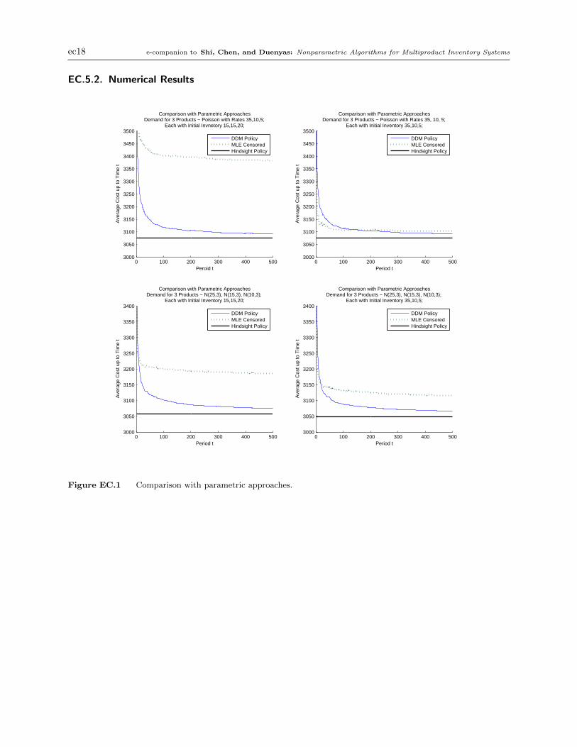
Comparison with parametric MLE algorithms. The numerical results are presented in Figure

EC.1. Our results indicate that DDM performs very well, and is consistent (i.e., it converges to the

optimal solution). In contrast, MLE Censored is significantly slower than DDM, and also suffers

from inconsistency, i.e., it often fails to converge to the optimal solution. This is due to a spiral-

down effect. More specifically, if the initial inventory level is lower than the optimal target level,

the censored demand is likely to give an even lower estimate in the next period (because the firm

cannot observe the lost-sales quantity). Then the target inventory level will be set lower and lower,

resulting in divergent cost. The consistency of MLE Censored hinges on the (almost) perfect initial

estimation of target levels, which is often impractical. In fact, in three of the examples in Figure

EC.1, the MLE Censored algorithm did not converge; in the only one where it did converge, we

actually picked starting target levels close enough to the optimal levels so that it would converge,

which of course would not be possible in practice.

Comparison with nonparametric algorithms. The numerical results are presented in Figure

EC.2. Our results show that DDM consistently outperforms both the B-S policy and the CAVE

policy. We also find out that the B-S policy has an extremely slow convergence rate while the CAVE

policy is much faster but still slower than DDM. Figure EC.2 also displays the performance of the

Uncensored SAA policy (assuming the uncensored demand information). It is interesting to note

that the DDM policy performs very close to the Uncensored SAA policy in all of our examples.

Extreme cases with uneven lost-sales penalty costs. DDM performs consistently very well

for extreme cases with some pathological parameters (see Figure EC.3).

Supplemental Material

An electronic companion to this paper is available at http://or.journal.informs.org/.

Acknowledgments

The authors are grateful to the area editor Professor Chung-Piaw Teo, the anonymous associate editor, and

the three anonymous referees for their detailed comments and suggestions, which have helped to significantly

improve both the content and the exposition of this paper. We thank Huseyin Topaloglu for sharing the CAVE

implementation. This research is partially supported by NSF grants CMMI-1362619 and CMMI-1451078.

Shi, Chen, and Duenyas: Nonparametric Algorithms for Multiproduct Inventory Systems 16

References

Bertsekas, D. P. 2000. Dynamic Programming and Optimal Control . 2nd ed. Athena Scientific.

Bertsekas, D. P., S. E. Shreve. 2007. Stochastic Optimal Control: The Discrete-Time Case. Athena Scientific.

Besbes, O., A. Muharremoglu. 2013. On implications of demand censoring in the newsvendor problem. Management Science

59(6) 1407–1424.

Beyer, D., S. P. Sethi, R. Sridhar. 2001. Stochastic multi-product inventory models with limited storage. Journal of Optimization

Theory and Applications 111 553–588.

Beyer, D., S. P. Sethi, R. Sridhar. 2002. Average-cost optimality of a base-stock policy for a multi-product inventory model with

limited storage. G. Zaccour, ed., Decision & Control in Management Science, Advances in Computational Management

Science, vol. 4. Springer US, 241–260.

Bookbinder, J. H., A. E. Lordahl. 1989. Estimation of inventory re-order levels using the bootstrap statistical procedure. IIE

Transactions 21(4) 302–312.

Boyd, S., L. Vandenberghe. 2004. Convex Optimization. Cambridge University Press, New York, NY, USA.

Burnetas, A. N., C. E. Smith. 2000. Adaptive ordering and pricing for perishable products. Operations Research 48(3) 436–443.

Chen, L., E. L. Plambeck. 2008. Dynamic inventory management with learning about the demand distribution and substitution

probability. Manufacturing & Service Operations Management 10(2) 236–256.

Choi, J., J. J. Cao, H. E. Romeijn, J. Geunes, S. X. Bai. 2005. A stochastic multi-item inventory model with unequal replen-

ishment intervals and limited warehouse capacity. IIE Transactions 37(12) 1129–1141.

Chu, L. Y., J. G. Shanthikumar, Z.-J. M. Shen. 2008. Solving operational statistics via a bayesian analysis. Operations Research

Letters 36(1) 110 – 116.

Flaxman, A. D., A. T. Kalai, H. B. McMahan. 2005. Online convex optimization in the bandit setting: Gradient descent without

a gradient. Proceedings of the Sixteenth Annual ACM-SIAM Symposium on Discrete Algorithms. SODA ’05, 385–394.

Glasserman, P. 1991. Gradient Estimation Via Perturbation Analysis. Kluwer international series in engineering and computer

science: Discrete event dynamic systems, Springer.

Godfrey, G. A., W. B. Powell. 2001. An adaptive, distribution-free algorithm for the newsvendor problem with censored

demands, with applications to inventory and distribution. Management Science 47(8) 1101–1112.

Hazan, E. 2015. Introduction to online convex optimization. Book Draft. Computer Science, Princeton University. Available

at http://ocobook.cs.princeton.edu/OCObook.pdf.

Hazan, E., A. Kalai, S. Kale, A. Agarwal. 2006. Logarithmic regret algorithms for online convex optimization. In 19th COLT .

499–513.

Huh, W. H., P. Rusmevichientong. 2009. A non-parametric asymptotic analysis of inventory planning with censored demand.

Mathematics of Operations Research 34(1) 103–123.

Huh, W. H., P. Rusmevichientong, R. Levi, J. Orlin. 2011. Adaptive data-driven inventory control with censored demand based

on kaplan-meier estimator. Operations Research 59(4) 929–941.

Huh, W. T., G. Janakiraman, J. A. Muckstadt, P. Rusmevichientong. 2009. An adaptive algorithm for finding the optimal

base-stock policy in lost sales inventory systems with censored demand. Mathematics of Operations Research 34(2)

397–416.

Ignall, E., A. F. Veinott. 1969. Optimality of myopic inventory policies for several substitute products. Management Science

15(5) 284–304.

Kleywegt, A. J., A. Shapiro, T. Homem-de Mello. 2002. The sample average approximation method for stochastic discrete

optimization. SIAM J. on Optimization 12(2) 479–502.

Kunnumkal, S., H. Topaloglu. 2008. Using stochastic approximation methods to compute optimal base-stock levels in inventory

control problems. Operations Research 56(3) 646–664.

Shi, Chen, and Duenyas: Nonparametric Algorithms for Multiproduct Inventory Systems 17

Lariviere, M. A., E. L. Porteus. 1999. Stalking information: Bayesian inventory management with unobserved lost sales.

Management Science 45(3) 346–363.

Levi, R., G. Perakis, J. Uichanco. 2015. The data-driven newsvendor problem: New bounds and insights. Operations Research

63(6) 1294–1306.

Levi, R., R. O. Roundy, D. B. Shmoys. 2007. Provably near-optimal sampling-based policies for stochastic inventory control

models. Mathematics of Operations Research 32(4) 821–839.

Liyanage, L. H., J. G. Shanthikumar. 2005. A practical inventory control policy using operational statistics. Operations Research

Letters 33(4) 341 – 348.

Loulou, R. 1978. An explicit upper bound for the mean busy period in a GI/G/1 queue. Journal of Applied Probability 15(2)

452–455.

Maglaras, C., S. Eren. 2015. A maximum entropy joint demand estimation and capacity control policy. Production and

Operations Management 24(3) 438–450.

Nemirovski, A., A. Juditsky, G. Lan, A. Shapiro. 2009. Robust stochastic approximation approach to stochastic programming.

SIAM J. on Optimization 19(4).

Powell, W., A. Ruszczynski, H. Topaloglu. 2004. Learning algorithms for separable approximations of discrete stochastic

optimization problems. Mathematics of Operations Research 29(4) 814–836.

Shaked, M., J. G. Shanthikumar. 2007. Stochastic Orders. Springer Series in Statistics, Physica-Verlag.

Shalev-Shwartz, S. 2012. Online learning and online convex optimization. Found. Trends Mach. Learn. 4(2) 107–194.

Veinott, Jr., A. F. 1965. Optimal policy for a multi-product, dynamic, nonstationary inventory problem. Management Science

12(3) pp. 206–222.

Zinkevich, M. 2003. Online convex programming and generalized infinitesimal gradient ascent. Tom Fawcett, Nina Mishra, eds.,

Proceedings of the 20th International Conference on Machine Learning (ICML). AAAI Press, Cambridge, MA, USA,

928–936.

Zipkin, P. 2000. Foundations of Inventory Management . McGraw-Hill, New York.

Brief Bio:

Cong Shi is an assistant professor in the Department of Industrial and Operations Engineering

at the University of Michigan. His research lies in stochastic optimization and online learning theory

with applications to inventory and supply chain management, and revenue management. He won

first prize in the 2009 George Nicholson Student Paper Competition.

Weidong Chen is a Ph.D. candidate in the Department of Industrial and Operations Engineer-

ing at the University of Michigan. His research lies in stochastic optimization and online learning

theory with applications to inventory and supply chain management, and revenue management.

Izak Duenyas is the Donald C. Cook Professor of Business Administration and Professor

of Technology and Operations at the Ross School of Business. His recent research interests are

in pricing and revenue management, sourcing and procurement, and production, inventory and

capacity control.

e-companion to Shi, Chen, and Duenyas: Nonparametric Algorithms for Multiproduct Inventory Systems ec1

This page is intentionally blank. Proper e-companion title

page, with INFORMS branding and exact metadata of the

main paper, will be produced by the INFORMS office when

the issue is being assembled.

ec2 e-companion to Shi, Chen, and Duenyas: Nonparametric Algorithms for Multiproduct Inventory Systems

Electronic Companion to

“Nonparametric Data-Driven Algorithms for Multi-Product

Inventory Systems with Censored Demand”

Cong Shi∗, Weidong Chen∗, Izak Duenyas†

∗ Industrial and Operations Engineering, University of Michigan, {shicong, aschenwd}@umich.edu

† Technology and Operations, Ross School of Business, University of Michigan, duenyas@umich.edu

EC.1. Clairvoyant Optimal Policy – Proof of Theorem 1

Based on (3), we define a myopic feasible (closed-loop) policy π as a sequence of functions yt =

πt(xt), t = 1, . . . , T , mapping beginning inventory (state) xt into ending inventory (decision) yt,

which also “myopically” minimizes per-period cost Πt(·) with beginning inventory xt, i.e.,

yt(xt), arg mina∈Γ:a≥xt

Πt(a). (EC.1)

The above feasible policy π is myopic, because it only optimizes per-period cost in each period

(the immediate reward). This is in contrast with standard dynamic programming or approximate

dynamic programming approaches. To ease the presentation of establishing optimality of π, fol-

lowing Ignall and Veinott (1969), we keep xt, yt, Πt time-generic, i.e.,

y(x), arg mina∈Γ:a≥x

Π(a). (EC.2)

It is important to see that y(x) is the unique minimizer of (EC.2), due to Assumption 1 ensuring

strict (joint) convexity of Π(y) over the feasible region, and the fact that the constraint set is affine

(see Boyd and Vandenberghe (2004)).

Lemma EC.1. The optimization problem defined in (EC.2) has a unique minimizer y(x).

Proof of Lemma EC.1. Due to Assumption 1, the cost function Π(·) is differentiable and finite-

valued. The derivatives inside expectation are bounded, and also the expectation is a multiple

integration over finite ranges. Hence this guarantees the validity of interchange between differenti-

ation and expectation.

Next we argue that Π(·) are strictly (jointly) convex over the feasible region. For all i and j,

∂2Π(a)

∂(ai)2= (hi + pi− ci)F ′Di(a

i)> 0;∂2Π(a)

∂ai∂aj= 0,

e-companion to Shi, Chen, and Duenyas: Nonparametric Algorithms for Multiproduct Inventory Systems ec3

where Assumption 1(c) ensures F ′Di

(ai)> 0 for all ai ∈ [0,M ]. Hence, the Hessian matrix is positive

definte (with all strictly positive eigenvalues) over the entire feasible region, ensuring Π to be

strictly (jointly) convex.

Now consider the optimization problem (with a given starting inventory x) defined in (EC.2).

Since Π(y) is strictly (jointly) convex and the constraint set is affine, y(x) is the unique minimizer.

(See Boyd and Vandenberghe (2004) for discussions of unique minimizer in convex optimization

problems and also Example 5.4.). Q.E.D.

Next we shall show that the myopic policy π defined above is optimal. Ignall and Veinott (1969)

provided a sufficient condition called substitute property (together with two mild regularity assump-

tions) under which the myopic policy is optimal.

Definition EC.1 (Substitute property). For any inventory levels x, x∈ Γ,

if x≥ x, then y(x)−x≤ y(x)− x.

Definition EC.2 (Regularity conditions in Ignall and Veinott (1969)). The two reg-

ularity conditions in Ignall and Veinott (1969) are: (a) x ≤ x′ ≤ y(x) implies y(x) = y(x′) for

x,x′ ∈ Γ; (b) The state transition permits either pure, partial, or no backlogging (lost-sales).

The regularity condition (a) is satisfied by y(x) being the unique minimizer of (EC.2) by Lemma

EC.1, and the regularity condition (b) is immediate since we consider a standard lost-sales model.

We can now proceed to establish the optimality of myopic policies for the multi-product lost-

sales system by showing that the sufficient condition (substitute property) given above holds for

our system.

Proposition EC.1. Under Assumption 1, when the demand distribution is known a priori, the

myopic ordering policy defined in (EC.1) is optimal for the multi-product lost-sales inventory sys-

tems.

To prove Proposition EC.1, we need to derive several important properties of the myopic pol-

icy. Now consider the two possible starting inventory levels x and x, with x ≥ x. For notational

(superscript) convenience, we use θ instead of y∗ to be the global minimizer of Π(·) over Γ. Recall

that θ = y∗ , arg mina∈Γ Π(a), and also the myopic order-to-up level y(x) , arg mina∈Γ:a≥x Π(a).

For simplicity, we define the boundary of our warehouse storage constraint,

∂Γ,

{y ∈Rn+ :

n∑i=1

yi =M

}.

ec4 e-companion to Shi, Chen, and Duenyas: Nonparametric Algorithms for Multiproduct Inventory Systems

Note that y ∈ ∂Γ means that the total order-up-to levels have reached the total storage limit M .

If y /∈ ∂Γ, then the warehouse storage constraint is not tight.

Now denote the jth partial derivative of Π(·) by Π′j(·). We then develop some useful properties

of the myopic order-up-to levels y(·).

Lemma EC.2. Let x∈ Γ and θ be the global minimizer of Π(·) over Γ,

(i) xj ≥ θj⇒ yj(x) = xj.

(ii) xj ≤ θj⇒ yj(x)≤ θj.

Proof of Lemma EC.2. The proof is straightforward. Statement (i) holds because xj ≥ θj (the

starting inventory is higher than the global minimizer) for product j, it is sub-optimal to order any

more product j. Statement (ii) holds because if xj ≤ θj (the starting inventory is lower than the

global minimizer), it is sub-optimal to raise the inventory above the global minimizer. Q.E.D.

Lemma EC.3. Let x∈ Γ and θ be the global minimizer of Π(·) over Γ,

(i) θ ∈ ∂Γ⇒ y(x)∈ ∂Γ;

(ii) y(x) /∈ ∂Γ, xj ≤ θj⇒ yj(x) = θj.

In Lemma EC.3, statement (i) states that if the global minimizer occupies the entire storage

space, then the myopic order-up-to levels will also occupy the entire storage space. This is because

our myopic policy will always order as much as possible to approach the global minimizer. Statement

(ii) states that if the total myopic order-up-to level has not reached the storage limit M , then if

xj ≤ θj, the myopic policy will raise inventory level for product j to the global minimizer θj.

Proof of Lemma EC.3. We prove (i) by contradiction. Suppose that θ ∈ ∂Γ and y(x) /∈ ∂Γ, then

n∑i=1

θi =M andn∑i=1

yi(x)<M.

It is obvious that there exists at least one j such that yj(x)< θj. Since θ minimizes Π(·) over Γ, it

is clear that θ either reaches the global minimizer of Π(·) over the entire real line R or is smaller

than it due to the storage constraint, so the derivative Π′j(θ)≤ 0. Therefore, since Π(·) is strictly

convex,

Π′j(y(x))<Π′j(θ)≤ 0.

On the other hand, since y(x) /∈ ∂Γ and y(x) is a minimizer of Π(·) over set {y | y≥ x,y ∈ Γ}, it

is clear that y(x) either reaches θ or is greater than it because of the initial on-hand inventory, so

Π′j(y(x))≥ 0, which results in a contradiction, thereby proving (i).

To prove (ii), we observe from the contraposition of (i), i.e., y(x) /∈ ∂Γ⇒ θ /∈ ∂Γ. Then for any

product j, yj(x) is not restricted by the storage constraint, and thus if θj ≥ xj, then θj can always

be reached, implying that yj(x) = θj. This completes the proof. Q.E.D.

e-companion to Shi, Chen, and Duenyas: Nonparametric Algorithms for Multiproduct Inventory Systems ec5

Lemma EC.4. yj(x)>xj⇒Π′j(y(x)) = miniΠ′i(y(x))

Lemma EC.4 states that if a product is ordered, then the marginal cost of any additional ordering

must be equal across the products. Intuitively, if the marginal cost of ordering this product is

higher than others, we can always reduce the quantity of this product and order more of the other

products. The rigorous proof is as follows.

Proof of Lemma EC.4. We prove this result by contradiction. Suppose that there exists an i,

1 ≤ i ≤ n, such that Π′i(y(x)) < Π′j(y(x)). Then, for a sufficiently small ε > 0, (y1(x), ...yj(x) −

ε, ..., yi(x) + ε, ..., yn(x))∈ Γ, and we have

Π(y(x))−Π(y1(x), ...yj(x)− ε, ..., yi(x) + ε, ..., yn(x))

= ε(Π′j(y(x))−Π′i(y(x))) + o(ε2)> 0,

which contradicts to the fact that y(x) minimizes Π(·) over set {y | y≥ x,y ∈ Γ}. Q.E.D.

Now, we are ready to prove Proposition EC.1.

Proof of Proposition EC.1. To establish the optimality of myopic policies for the multi-product

lost-sales system, it suffices to verify that the substitute property (EC.1) holds, i.e., for any inven-

tory levels x, x∈ Γ, if x≥ x, then y(x)−x≤ y(x)− x.

We know that the myopic order-up-to levels yj(x) ≥ xj for any product j if x ∈ Γ. Similarly,

yj(x)≥ xj for any product j if x∈ Γ. Now if yj(x) = xj, then we have

0 = yj(x)−xj ≤ yj(x)− xj.

Thus, it suffices to prove that yj(x)≤ yj(x), whenever yj(x)>xj. We have to consider three cases

as follows.

Case (a). First, if both y(x) /∈ ∂Γ and yj(x) /∈ ∂Γ, then it follows from Lemma EC.2 and Lemma

EC.3 that

yj(x) = max{θj, xj}, yj(x) = max{θj, xj}, ∀ j.

Then yj(x) = yj(x) and the result follows immediately.

Case (b). Second, if y(x)∈ ∂Γ but yj(x) /∈ ∂Γ, then by Lemma EC.2 (ii) and Lemma EC.3 (ii),

we have yj(x)≤ θj = yj(x), and the result also follows immediately. It is impossible for the case

where y(x) /∈ ∂Γ and yj(x)∈ ∂Γ to happen. To see this, if such case exists, then we can always find

some j such that for xj > xj, yj(x)> yj(x). However, by Lemma EC.2 (ii) and Lemma EC.3 (ii),

we know that yj(x)≤ θj = yj(x), which results in a contradiction.

ec6 e-companion to Shi, Chen, and Duenyas: Nonparametric Algorithms for Multiproduct Inventory Systems

Case (c). Third, we need to analyze the remaining case where y(x)∈ ∂Γ and yj(x)∈ ∂Γ, i.e.,

n∑j=1

yj(x) =n∑j=1

yj(x) =M. (EC.3)

We partition all the products into three sets as follows,

Ia = {k : yk(x)>xk}, Ib = {k : yk(x) = xk ∩Π′k(yk(x)≤ 0}, Ic = {k : Π′k(y

k(x)> 0}.

Note that these three sets are disjoint and the union of them is exhaustive.

Now we focus on the set Ic first and let j ∈ Ic. Then we have yj(x)≥max{xj, θj}. By Lemma

EC.2, it is clear that yj(x) ≤max{xj, θj}. Hence, yj(x)− yj(x) ≤ 0 for all j ∈ Ic. Together with

(EC.3), we know thatn∑

j∈Ia∪Ib

(yj(x)− yj(x)

)≥ 0.

If ym(x) = ym(x) for all m ∈ Ia ∪ Ib, then the result follows immediately. Now consider the case

where there exists a product m ∈ Ia ∪ Ib such that ym(x) > ym(x). This implies that ym(x) >

ym(x)≥ xm ≥ xm ≥ 0. By Lemma EC.4, we have Π′m(y(x)) = miniΠ′i(y(x)). Moreover, due to the

strict convexity of Π(·), then we have

mini

Π′i(y(x)) = Π′m(y(x))>Π′m(y(x)). (EC.4)

To complete the proof, it suffices to show that for any product j ∈ Ia, yj(x)≥ yj(x). Now suppose

there exists a product n∈ Ia such that yn(x)< yn(x). It is clear that yn(x)> yn(x)≥ 0. By Lemma

EC.4, we have Π′n(y(x)) = miniΠ′i(y(x)). Moreover, due to the strict convexity of Π(·), then we

have

mini

Π′i(y(x)) = Π′n(y(x))>Π′n(y(x)). (EC.5)

Note that (EC.4) implies that Π′n(y(x))>Π′m(y(x)) but (EC.5) implies that Π′m(y(x))>Π′n(y(x)),

which results in a contradiction. This completes the proof. Q.E.D.

Equipped with Proposition EC.1, we are ready to prove Theorem 1.

Proof of Theorem 1. Proposition EC.1 fully characterizes the structural properties of optimal

policies as follows. Let y∗ be a unique critical (deterministic) vector defined by in (4). Then a

clairvoyant optimal policy π∗ is characterized as follows:

(a) If the beginning inventory level of product i is above its individual base-stock level (i.e., the

ith component of y∗), then this product is not ordered in the period.

(b) If this product i is ordered in the period, the ending inventory level (after ordering) does not

exceed its individual base-stock level (i.e., the ith component of y∗).

e-companion to Shi, Chen, and Duenyas: Nonparametric Algorithms for Multiproduct Inventory Systems ec7

(c) If there is enough storage space to bring all products (whose inventory levels are below their

individual base-stock levels) up to their base-stock levels, then such an order is optimal. Oth-

erwise, the ending inventory levels takes up all the available storage space.

Thus, the stationary multi-period inventory problem is analytically equivalent to the single-period

problem, and ordering up to y∗ in each period is also optimal for this problem. Clearly, once we

start below y∗, and order up to y∗, we remain at or below y∗ thereafter; in such a case, the expected

cost incurred in each period is Π(y∗). Q.E.D.

EC.2. Proof of Lemma 1 - Online Convex Optimization

Proof of Lemma 1. Due to convexity of the cost function Π(y), we have

E [Π(yt)−Π(y∗)]≤E [∇Π(yt)(yt−y∗)] . (EC.6)

Note that the subgradient ∇Π(yt) defines the supporting hyperplane of Π at the point yt.

For any period t∈ T , i.e., in the set of break points, we can obtain the upper bound of the second

moment difference between our target inventory level and the optimal target inventory level.

E||yt+1−y∗||2 ≤ E||zt+1−y∗||2 (EC.7)

= E||yt− ηtGt(yt)−y∗||2

= E||yt−y∗||2 + η2tE||Gt(yt)||2− 2ηtE[Gtn(yt)(yt−y∗)],

where the first inequality follows the optimization (7) and the Pythagorean Theorem since

||zt+1−y∗||2 = ||yt+1−y∗||2 + ||zt+1− yt+1||2

by property of the 2-norm projection; the first equality follows from the definition of zt+1; the

second equality follows from a simple binomial expansion.

We can also re-write E[Gt(yt)(yt−y∗)] by taking conditional expectation on the value of yt,

E [Gt(yt)(yt−y∗)] = E [E [Gt(yt)(yt−y∗)|yt]] (EC.8)

= E [E [Gt(yt)|yt] (yt−y∗)]

= E [∇Π(yt)(yt−y∗)] ,

where the first equality holds because y∗ does not relate with yt; the last equality follows from the

fact that Gt is an unbiased estimator of the true gradient ∇Π.

ec8 e-companion to Shi, Chen, and Duenyas: Nonparametric Algorithms for Multiproduct Inventory Systems

Combining (EC.7) and (EC.8), it is clear that

E[∇Π(yt)(yt−y∗)]≤ 1

2ηt

(E||yt−y∗||2−E||yt+1−y∗||2

)+ηt2E||Gt(yt)||2. (EC.9)

Without loss of generality, let T = {τ0, . . . , τk} with τ0 = 0 and τk = T . By the construction of DDM,

E

[T∑t=1

Π(yt)−T∑t=1

Π(y∗)

]=E

[k−1∑s=0

τs+1∑t=τs+1

(Π(yt)−Π(y∗))

]≤ M

l·E

[k∑s=1

(Π(yτs)−Π(y∗))

],

where the inequality follows from the fact that the time between any two consecutive break points

cannot exceed the time for a “fictitious” system with M inventory units for each product i= 1, . . . , n

to become empty along every sample path. The expectation of the latter (which is independent of

yt) is upper bounded by M/l.

It then suffices to bound the term E[∑k

s=1 (Π(yτs)−Π(y∗))]. Now, by summing both sides of

(EC.6) over periods τ1 to τk,

E

[k∑s=1

(Π(yτs)−Π(y∗))

]≤

k∑s=1

E [∇Π(yτs)(yτs −y∗)] (EC.10)

≤k∑s=1

(1

2ητs

(E||yτs −y∗||2−E||yτs+1−y∗||2

)+ητs2E||Gτs(yτs)||2

)

=k∑s=1

(1

2ητs

(E||yτs −y∗||2−E||yτs+1

−y∗||2)

+ητs2E||Gτs(yτs)||2

)

=1

2ητ1E||yτ1 −y∗||2− 1

2ητkE||yτk+1

−y∗||2 +1

2

k∑s=2

(1

ητs− 1

ητs−1

)E||yτs −y∗||2

+k∑s=1

ητsE||Gτs(yτs)||2

2

≤ 2M 2

(1

2ητ1+

1

2

k∑s=2

(1

ητs− 1

ητs−1

))+n(maxi{pi− ci, hi})2

2

k∑s=1

ητs

=M 2

ητk+n(maxi{pi− ci, hi})2

2

k∑s=1

ητs ,

where the first and second inequalities follows from (EC.6) and (EC.9), respectively; the first

equality holds since yτs+1 = yτs+1by the construction of DDM; the last inequality follows from the

fact that for any x,y ∈ Γ,

||x−y||22 ≤ ||x||22 + ||y||22 ≤ ||x||21 + ||y||21 ≤ 2M 2.

e-companion to Shi, Chen, and Duenyas: Nonparametric Algorithms for Multiproduct Inventory Systems ec9

Putting everything together, we have

E

[T∑t=1

Π(yt)−T∑t=1

Π(y∗)

]≤ M

l

(M 2

ηT+n(maxi{pi− ci, hi})2

2

k∑s=1

ητs

). (EC.11)

Note that we have chosen our step size “optimally” as

ηt =

(γM√

n ·maxi{pi− ci, hi}

)1√t

for some γ > 0,

so that

k∑s=1

ητs ≤T∑t=1

ηt =

(γM√

n ·maxi{pi− ci, hi}

) T∑t=1

1√t≤(

γM√n ·maxi{pi− ci, hi}

)2√T . (EC.12)

Plugging (EC.12) and ηT into (EC.11) yields the result with the constant term

K1 = (γ+ γ−1)M 2l−1√n ·max

i{pi− ci, hi}.

Note that putting γ = 1 gives the tightest bound. This completes the proof. Q.E.D.

EC.3. Proof of Lemma 2 - Stochastic Dominance and a GI/G/1 Queue

Proof of Lemma 3. By the definition of the per-period cost function in (3), it follows that

E[Π(yt)−Π(yt)]≤E [c · (yt− yt)] +E[(h− c) · (yt− yt)

+]

+E[p · (yt−yt)

+]

= E[h · (yt− yt)

+]

+E[(p− c) · (yt−yt)

+]≤E [(h∨ (p− c) · |yt− yt|] ,

where the last inequality follows from various operators defined at the end of Section 1. Q.E.D.

Proof of Lemma 4. Case 1. We first consider time period t ∈ T = {τ0, . . . , τk}, which belongs

to the set of break points in DDM. Due to the construction of DDM, we update the target levels

at t+ 1 only if t ∈ T . For each product i ∈ J , i.e., xit+1 > yit+1, we have yit+1 = xit+1 > yit+1 ≥ 0 by

(9). This implies that yit+1 > 0, and by the lost-sales system dynamics, we have

xit+1 = (yit− dt)+ = yit− dt > 0. (EC.13)

The next key step is to compare the target level yit+1 with the constraint-free target level zit+1.

First, notice that when yit − dit > 0, the algorithm updates the constraint-free target level in a

negative direction, i.e.,

zit+1 = yit− ηthi < yit. (EC.14)

ec10 e-companion to Shi, Chen, and Duenyas: Nonparametric Algorithms for Multiproduct Inventory Systems

Second, by the important property (12) of our algorithm, we have

yjt+1 ≤ yjt + ηt

(pj − cj

), ∀ j = 1, . . . , n.

Thus, the maximum positive displacement of yt+1 from yt (excluding the set J) is

∑j∈J

(yjt+1− y

jt

)≤∑j∈J

ηt(pj − cj

). (EC.15)

Now, to draw a relation between yit+1 and zit+1, there are two cases.

Subcase 1a. In the first case where∑n

j=1 yjt+1 ≥

∑n

j=1 yjt , we must have

∑i∈J

(zit+1− yit+1

)<∑i∈J

(yit− yit+1

)≤∑j∈J

(yjt+1− y

jt

)≤∑j∈J

ηt(pj − cj

), (EC.16)

where the first inequality follows from (EC.14); the second inequality follows from∑n

j=1 yjt+1 ≥∑n

j=1 yjt ; and the third inequality follows from (EC.15).

Subcase 1b. In the second case where∑n

j=1 yjt+1 <

∑n

j=1 yjt ≤M , the warehouse storage con-

straint is not tight (i.e., the constraint-free target levels are in the interior of Γ), and by the

optimization procedure (10), zjt+1 = yjt+1 for all j = 1, . . . , n. Thus, we have

zit+1− yit+1 = yit+1− yit+1 = 0, i= 1, . . . , n. (EC.17)

Combining the above two cases and using the relations (EC.16) and (EC.17), we can then obtain

an upper bound for our distance function as follows,

∑i∈J

|yit+1− yit+1| =∑i∈J

(xit+1− yit+1

)=∑i∈J

(yit− dit− yit+1

)≤∑i∈J

(yit− dit− zit+1

)+∑j∈J

ηt(pj − cj

)=∑i∈J

(yit− yit

)+ ηt

∑i∈J

hi +∑j∈J

(pj − cj

)−∑i∈J

dit,

≤∑i∈J

∣∣yit− yit∣∣+ ηt

∑i∈J

hi +∑j∈J

(pj − cj

)−∑i∈J

dit,

where the first equality follows from the fact that i∈ J and the construction of our algorithm (9);

the second equality is due to (EC.13); the first inequality follows from (EC.16) and (EC.17), and

the third equality follows from (EC.14). Now we have completed the proof for Case 1.

Case 2. We then consider time period t /∈ T , which does not belong to the set of break points

in DDM. According to the construction of DDM, the target order-up-to levels are kept unchanged,

e-companion to Shi, Chen, and Duenyas: Nonparametric Algorithms for Multiproduct Inventory Systems ec11

i.e., yit+1 = yit for all i= 1, . . . , n and for all t /∈ T . we can similarly obtain an upper bound for our

distance function as follows,

∑i∈J

|yit+1− yit+1| =∑i∈J

(xit+1− yit+1

)=∑i∈J

(yit− dit− yit+1

)=∑i∈J

(yit− dit− yit

)≤∑i∈J

∣∣yit− yit∣∣−∑i∈J

dit,

where the first equality follows from the fact that i ∈ J and the construction of our algorithm

(9); the second equality is due to (EC.13); the third equality follows from yit+1 = yit. Now we have

completed the proof for Case 2. Q.E.D.

Proof of Lemma 5. Case 1. We first consider time period t ∈ T = {τ0, . . . , τk}, which belongs

to the set of break points in DDM. Due to the construction of DDM, we update the target levels

at t+ 1 only if t ∈ T . For each product i ∈ J , i.e., xit+1 ≤ yit+1, recall that we need to solve the

optimization problem (10) to determine our actual implemented levels yt+1. That is,

min∑i∈J

(yit+1− yit+1)2 s.t.∑i∈J

yit+1 ≤M −∑j∈J

xjt+1, yit+1 ≥ xit+1, ∀ i∈ J .

It is straightforward to see that yit+1 ≥ yit+1 for each product j ∈ J . To see this, suppose otherwise

yit+1 < yit+1; we can always lower the value of yit+1 to yit+1 strictly improving the objective value

while maintaining feasibility.

Now there are three sub-cases.

Subcase 1a. The simplest case is when J = ∅, then (10) reduces to

minn∑i=1

(yit+1− yit+1)2 s.t.∑i∈J

yit+1 ≤M, yit+1 ≥ xit+1, ∀ i∈ J .

Since yt+1 ∈ Γ, we have yit+1 = yit+1 for each product i= 1, . . . , n, and thus the distance function is

zero for each product i= 1, . . . , n.

Subcase 1b. The second case is when upon solving yt+1, the warehouse storage constraint is

not tight, i.e., ∑i∈J

yit+1 <M −∑j∈J

xjt+1. (EC.18)

Then we claim that ∑i∈J

yit+1 <M −∑j∈J

xjt+1, (EC.19)

ec12 e-companion to Shi, Chen, and Duenyas: Nonparametric Algorithms for Multiproduct Inventory Systems

We argue the claim by contradiction. Suppose otherwise that

∑i∈J

yit+1 ≥M −∑j∈J

xjt+1 >∑i∈J

yit+1.

Then there must exist a product k such that ykt+1 < ykt+1, you can always increase ykt+1 by

ε,M −∑j∈J

xjt+1−∑i∈J

yit+1 > 0

to make the warehouse storage constraint tight, thereby strictly reducing the optimal objective

value. This contradicts the optimality of yt+1 in (10).

Thus, by (EC.18) and (EC.19), we have yit+1 = yit+1 for each product i ∈ J , and the distance

function is zero for each product i= 1, . . . , n.

Subcase 1c. The third case is much more involved. That is, upon solving yt+1, the warehouse

storage constraint becomes tight, i.e.,

∑i∈J

yit+1 =M −∑j∈J

xjt+1,

and the set J 6= ∅. We can then rewrite the optimization problem (10) as follows,

min∑i∈J

(yit+1− yit+1)2 s.t.∑i∈J

(yit+1− yit+1

)=∑i∈J

yit+1−M +∑j∈J

xjt+1, yit+1 ≥ xit+1, ∀ i∈ J .

We then bound the distance function as follows,

∑i∈J

∣∣yit+1− yit+1

∣∣ =∑i∈J

yit+1−M +∑j∈J

xjt+1 =∑i∈J

yit+1−M +∑j∈J

(yjt − djt)+

=∑i∈J

yit+1−M +∑j∈J

(yjt − djt) =∑i∈J

yit+1−

(M −

∑j∈J

yjt

)−∑j∈J

djt

≤∑i∈J

yit+1−∑i∈J

yit−∑j∈J

djt =∑i∈J

(yit+1− yit

)−∑j∈J

djt

≤∑i∈J

(yit + ηt(p

i− ci)− yit)−∑j∈J

djt

≤∑i∈J

(yit− yit

)+∑i∈J

ηt(pi− ci)−

∑j∈J

djt

≤∑i∈J

∣∣yit− yit∣∣+ ηt∑i∈J

(pi− ci)−∑j∈J

djt ,

where the first equality is because the warehouse storage constraint becomes tight; the second

equality is due to the system dynamics; the third equality is because j ∈ J implies that xjt+1 > 0,

e-companion to Shi, Chen, and Duenyas: Nonparametric Algorithms for Multiproduct Inventory Systems ec13

and hence the plus sign can be removed; the first inequality is due to the fact that

∑j∈J

yjt +∑j∈J

yjt =n∑j=1

yjt ≤M ;

and the second inequality follows from the important property (12) of our algorithm. Now we have

completed the proof for Case 1.

Case 2. We then consider time period t /∈ T , which does not belong to the set of break points

in DDM. Due to the construction of DDM, the target order-up-to levels are kept unchanged, i.e.,

yit+1 = yit for all i= 1, . . . , n and for all t /∈ T . Also, if t /∈ T , then the optimization problem (10) has

a nonzero objective value, which suggests that the warehouse storage constraint has to be tight.

We then similarly bound the distance function as follows,

∑i∈J

∣∣yit+1− yit+1

∣∣ =∑i∈J

yit+1−M +∑j∈J

xjt+1 =∑i∈J

yit+1−M +∑j∈J

(yjt − djt)+

=∑i∈J

yit+1−M +∑j∈J

(yjt − djt) =∑i∈J

yit+1−

(M −

∑j∈J

yjt

)−∑j∈J

djt

≤∑i∈J

yit+1−∑i∈J

yit−∑j∈J

djt =∑i∈J

(yit+1− yit

)−∑j∈J

djt

=∑i∈J

(yit− yit

)−∑j∈J

djt ≤∑i∈J

∣∣yit− yit∣∣−∑j∈J

djt ,

where we used the same arguments as in Subcase 1c and also the fact that yit+1 = yit for all i =

1, . . . , n if t /∈ T . Now we have completed the proof for Case 2. Q.E.D.

Proof of Lemma 6. By Lemma 4, we have

∑i∈J

|yit+1− yit+1| ≤

∑i∈J

∣∣yit− yit∣∣+ ηt

∑i∈J

hi +∑j∈J

(pj − cj

)−∑i∈J

dit

+

,

and by Lemma 5, we have

∑i∈J

|yit+1− yit+1| ≤

(∑i∈J

∣∣yit− yit∣∣+ ηt∑i∈J

(pi− ci)− minj=1,...,n

djt

)+

.

Combining the above two inequalities yields the result. Q.E.D.

Proof of Lemma 7. By Lemma 6, for each period t+ 1, the sum of distance functions

n∑i=1

|yit+1− yit+1| ≤

(n∑i=1

∣∣yit− yit∣∣+ ηt

n∑i=1

(hi + 2

(pi− ci

))− minj=1,...,n

djt

)+

.

ec14 e-companion to Shi, Chen, and Duenyas: Nonparametric Algorithms for Multiproduct Inventory Systems

In addition, we know that∑n

i=1 |yi0 − yi0|= 0 (since the policy starts with zero inventory). Thus,

by the definition of the stochastic process Zt+1, it is clear that∑n

i=1 |yit+1 − yit+1| ≤st Zt+1. This

implies that∑n

i=1 |yit+1− yit+1| ≤cx Zt+1, and then the result follows immediately. Q.E.D.

Proof of Lemma 8. By Lemma 7, it suffices to show that E[∑T

t=1Zt

]≤ 2E[B]S

√T . Recall that

Zt+1 =

[Zt +

St√t− Dt

]+

, Z0 = 0.

Let the random variable l(t) denote the index k in which Bk contains t, and it is clear that

Zt ≤t∑

s=1

Ss√s1[s∈Bl(t)

]a.s.

By summing Zt over periods 1 to T and taking expectation, we have

E

[T∑t=1

Zt

]≤ E

[T∑t=1

t∑s=1

Ss√s1[s∈Bl(t)

]]≤E

[T∑t=1

St√t

T∑s=1

1[s∈Bl(t)

]]

= E

[T∑t=1

St√tBl(t)

]=

T∑t=1

1√tE[B1]S ≤ 2E[B]S

√T .

This completes the proof. Q.E.D.

Proof of Lemma 2. Combining Lemma 3 and Lemma 8, we have

∆2(T ) = E

[T∑t=1

(Π(yt)−Π(yt))

]≤E

[T∑t=1

(h∨ (p− c)) · |yt− yt|

]

≤ maxi{pi− ci, hi}E

[T∑t=1

|yt− yt|

]= max

i{pi− ci, hi}E

[T∑t=1

n∑i=1

|yit− yit|

]≤ max

i{pi− ci, hi}

(2√TE[B]S

)=(

2maxi{pi− ci, hi}E[B]S

)√T .

Recall that E[B]≤ σαe

6β

σ3+ασ and S =

∑n

i=1 (hi + 2(pi− ci)) . Setting the constant

K2 = 2maxi{pi− ci, hi}σ

αe

6β

σ3+ασ

{n∑i=1

(hi + 2

(pi− ci

))}.

yields the result. This completes the proof. Q.E.D.

EC.4. Extensions

We present the detailed arguments to the following extensions of our model.

e-companion to Shi, Chen, and Duenyas: Nonparametric Algorithms for Multiproduct Inventory Systems ec15

EC.4.1. Different Product Dimensions or Sizes

We prove that by a cost transformation, this general model reduces to the basic model and hence

our results remain the same. We define new decision variables as follows,

yit = viyit, xit = vixit, qit = viqit,

for i= 1, . . . , n. In addition, we appropriately scale the demand and cost parameters as follows,

Dit = viDi

t, ci = ci/vi, hi = hi/vi, pi = pi/vi

for i = 1, . . . , n. With the above transformation, the cost of a feasible policy π under the new

warehouse-capacity constraint (14) can be transformed as follows,

C(π) = E

[T∑t=1

c · (yt−xt) + h · (yt−Dt)+ + p · (Dt−yt)

+

]−E[c ·xT+1], (EC.20)

= E

[T∑t=1

c · (yt− xt) + h · (yt− Dt)+ + p · (Dt− yt)

+

]−E[c · xT+1].

Moreover, it is clear that the new constraint defined in (14) is equivalent to

yt ∈ Γ,

{yt ∈Rn+ :

n∑i=1

yit ≤M

},

which has the same form as in the original constraint defined in (1). Hence, this more general

model has been reduced to the basic model. Our data-driven algorithm (now defined in terms of

transformed variables) and its performance analysis remain the same.

EC.4.2. Discrete Demand and Ordering Quantities

Data-Driven Multi-product Algorithm for Discrete Demands (DDM-Discrete).

Step 0. (Initialization.) Set the initial inventory levels y0 = y0 = y0 to be any non-negative integer

values within Γ and then set the initial values t= 0, τ0 = 0 and k= 0.

For each period t= 0, . . . , T − 1, repeat the following steps:

Step 1. (Setting the constraint-free and constrained target inventory levels.)

Case 1: If yt ≥ yt, the algorithm updates the constraint-free target inventory levels zt+1 by (5);

however, for each product i= 1, . . . , n, the ith component of Gt is defined as

Git(yt) =

−pi + cit + (hi + pi− ci) ·1(dit ≤ yit), if yit = byitc,

−pi + cit + (hi + pi− ci) ·1(dit ≤ yit− 1), if yit = dyite,(EC.21)

ec16 e-companion to Shi, Chen, and Duenyas: Nonparametric Algorithms for Multiproduct Inventory Systems

which is the right derivative of Π at byitc, i.e., the slope of Π at yit for the piece-wise linear cost.

Then the algorithm obtains an intermediate (continuous) target level yt+1 by solving yt+1 =

arg minw∈Γ ||w− zt+1||2. Then set the constrained (discrete) target inventory levels yt+1 by proba-

bilistic rounding. That is, if yit+1 is already an integer, set yit+1 = yit+1; otherwise, we flip a (biased)

coin with probability yit+1 − byit+1c of heads. Set yit+1 = dyit+1e if the outcome is head and set

yit+1 = byit+1c if the outcome is tail.

Record the break point τk := t+ 1 and increase the value k by 1.

Case 2: Else if yt � yt, the algorithm keeps both the constraint-free and constrained target

inventory levels unchanged, i.e., zt+1 = zt and yt+1 = yt.

Step 2. (Solving for the actual implemented target inventory levels.)

Define the set J and its complement as J ,{i : xit+1 > y

it+1

}and J ,

{i : xit+1 ≤ yit+1

}. For each

product i∈ J , we set the actual implemented levels yit+1 = xit+1 if xit+1 > yit+1.

If J 6= ∅, then we set the actual implemented levels yt+1 by solving

min∑i∈J

(yit+1− yit+1)2 s.t.∑i∈J

yit+1 ≤M −∑j∈J

xjt+1, yit+1 ≥ xit+1, y

it+1 ∈Z+, ∀ i∈ J . (EC.22)

This concludes the description of the algorithm.

Note that the key differences between DDM-Discrete and DDM are in Step 1 – defining a modified

gradient Gt, and probabilistic rounding. In order to establish our performance guarantee, we need

a lost-sales indicator for whether lost-sales has occurred in each period t, thereby determining the

value of 1(yit ≤ dit) . Without this indicator, it is not sufficient to obtain an unbiased estimator for

the right derivative of our cost function Π(·) by observing the past sales quantities. The decision

maker no longer has access to a local (stochastic) direction of cost improvement. For example, if

the computed target inventory level is 15.5 for some product i and we round it down to 15, even

an infinite number of sales observations would not allow the decision maker to obtain an estimate

of the slope of Πi(·) at 15.5. This is because if the demand turns out to be exactly 15, the unbiased

gradient should be hi since our target level 15.5 is higher than 15; however, if the demand turns out

to be 16, then the unbiased gradient should be −pi + ci. In both cases, we observe zero inventory

but cannot determine if the demand is strictly greater than 15 without a lost-sales indicator.

However, with access to this lost-sales indicator, we can construct such an estimator Gt defined in

(EC.21), which is unbiased when t∈ T . Then the proofs of bounds ∆1 and ∆2 are almost identical

to the ones used in DDM as long as the warehouse-capacity M is also an integer. Hence we are able

to extend our results to the discrete demand and inventory case as stated in the theorem below.

Theorem EC.1. Assume that the clairvoyant optimal solution in (EC.2) is unique in the discrete

demand case. With access to the lost-sales indicator, the average regret RT/T of our data-driven

e-companion to Shi, Chen, and Duenyas: Nonparametric Algorithms for Multiproduct Inventory Systems ec17

algorithm for discrete demand case (DDM-Discrete) approaches 0 at the rate of 1/√T . That is,

there exists some constant K, such that for any T ≥ 1,

1

TRT ,

1

TE

[T∑t=1

Π(yt)

]−Π(y∗)≤ K√

T.

To the best of our knowledge, the availability of the lost-sales indicator has been assumed in all

nonparametric studies that analyze newsvendor-type problems with an unknown discrete demand

distribution (see, e.g., Huh and Rusmevichientong (2009) and Besbes and Muharremoglu (2013)).

They showed that active exploration plays a much stronger role in the discrete case (compared to

the continuous case). However, the need for active exploration disappears as soon as a lost-sales

indicator (that records whether demand was censored or not) becomes available, in addition to the

censored demand samples. The access to this indicator allows the decision maker to obtain a noisy

signal about the potential need for an upward correction.

EC.5. Numerical Experiments

We present the setup of our numerical experiments and also the numerical results.

EC.5.1. Experimental Setup

For each experiment, we specify a (hindsight) demand distribution with cumulative distribution

function F (·). The lost-sales penalty cost pi for each product i is randomly drawn from the interval

[70,90] and the purchasing cost ci for each product i is randomly drawn from the interval [55,65].

We then set the holding cost hi = 0.02ci for each product i (see, e.g., Zipkin (2000)). To compare

the cost under each algorithm, we evaluate each algorithm on N = 200 randomly generated problem

instances. Each problem instance consists of independent demand samples and parameters over

a time horizon of 500 periods, unless specified otherwise. For each algorithm π, we compute the

average cost till period t, which is given by

1

N

N∑j=1

1

t

t∑s=1

Πj,s(yπj,s),

where the one-period cost Πj,s(y) in period s of the problem instance j is given by

Πj,s(y) =n∑i=1

ciyi,πj,s + (hi− ci)(yi,πj,s − dij,s)+ + pi(dij,s− yi,πj,s )+,

where dij,s is the demand realization for product i in period s of the problem instance j, and yi,πj,s

is the corresponding order-up-to level computed by each algorithm π.

ec18 e-companion to Shi, Chen, and Duenyas: Nonparametric Algorithms for Multiproduct Inventory Systems

EC.5.2. Numerical Results

0 100 200 300 400 5003000

3050

3100

3150

3200

3250

3300

3350

3400

3450

3500

Peroid t

Ave

rage

Cos

t up

to T

ime

tComparison with Parametric Approaches

Demand for 3 Products ~ Poisson with Rates 35,10,5; Each with Initial Invnetory 15,15,20;

0 100 200 300 400 5003000

3050

3100

3150

3200

3250

3300

3350

3400

3450

3500

Period t

Ave

rage

Cos

t up

to T

ime

t

Comparison with Parametric ApproachesDemand for 3 Products ~ Poisson with Rates 35, 10, 5;

Each with Initial Inventory 35,10,5;

0 100 200 300 400 5003000

3050

3100

3150

3200

3250

3300

3350

3400

Period t

Ave

rage

Cos

t up

to T

ime

t

Comparison with Parametric ApproachesDemand for 3 Products ~ N(25,3), N(15,3), N(10,3);

Each with Initial Inventory 15,15,20;

0 100 200 300 400 5003000

3050

3100

3150

3200

3250

3300

3350

3400

Period t

Ave

rage

Cos

t up

to T

ime

t

Comparison with Parametric ApproachesDemand for 3 Products ~ N(25,3), N(15,3), N(10,3);

Each with Initial Inventory 35,10,5;

DDM PolicyMLE CensoredHindsight Policy

DDM PolicyMLE CensoredHindsight Policy

DDM PolicyMLE CensoredHindsight Policy

DDM PolicyMLE CensoredHindsight Policy

Figure EC.1 Comparison with parametric approaches.

e-companion to Shi, Chen, and Duenyas: Nonparametric Algorithms for Multiproduct Inventory Systems ec19

0 100 200 300 400 5003100

3200

3300

3400

3500

3600

3700

3800

Period t

Ave

rage

Cos

t up

to T

ime

t

Comparison with Non−Parametric ApproachesDemand for 3 Products ~ Poisson with Rates 25, 15, 10; Initial Inventory 50, 0, 0

0 100 200 300 400 5003100

3200

3300

3400

3500

3600

3700

3800

Period t

Ave

rage

Cos

t up

to T

ime

t

Comparison with Non−Parametric ApproachesDemand for 3 Products ~ Poisson with Rates 30, 10, 10; Initial Inventory 50, 0, 0

0 100 200 300 400 5003000

3100

3200

3300

3400

3500

3600

3700

3800

Period t

Ave

rage

Cos

t up

to T

ime

t

Comparison with Non−Parametric ApproachesDemand for 3 Products ~ N(25,3), N(15,3), N(10,3); Initial Inventory 50, 0, 0

0 100 200 300 400 5003000

3100

3200

3300

3400

3500

3600

3700

3800

Period t

Ave

rage

Cos

t up

to T

ime

t

Comparison with Non−Parametric ApproachesDemand for 3 Products ~ N(30,3), N(10,3), N(10,3); Initial Inventory 50, 0, 0

Uncensored SAABS PolicyDDM PolicyCAVE PolicyHindsight Policy

Uncensored SAABS PolicyDDM PolicyCAVE PolicyHindsight Policy

Uncensored SAABS PolicyDDM PolicyCAVE PolicyHindsight Policy

Uncensored SAABS PolicyDDM PolicyCAVE PolicyHindsight Policy

Figure EC.2 Comparison with nonparametric approaches.

0 50 100 150 200 250 300 350 400 450 5003000

4000

5000

6000

7000

8000

9000

Period t

Ave

rage

Cos

t up

to T

ime

t

Extreme CasesDemand for 3 Products ~ Poisson with Rates 25,15,5

Uncensored SAABS PolicyDDM PolicyCAVE PolicyHindsight Policy

0 50 100 150 200 250 300 350 400 450 500

3000

4000

5000

6000

7000

8000

9000

Period t

Ave

rage

Cos

t up

to T

ime

t

Extreme CasesDemand for 3 Products ~ N(25,3), N(15,3), N(10,3)

Uncensored SAABS PolicyDDM PolicyCAVE PolicyHindsight Policy

Figure EC.3 Extreme cases with uneven lost-sales penalty costs p = [400,80,80].