Nonparametric Kernel Density Estimation Near the Boundary Peter Malec a,* , Melanie Schienle b a Institute for Statistics and Econometrics, Humboldt-Universit¨at zu Berlin, Spandauer Str. 1, D-10178 Berlin, Germany. b Institute for Empirical Economics, Leibniz University Hannover, K¨onigsworther Platz 1, D-30167 Hannover, Germany. Abstract Standard fixed symmetric kernel type density estimators are known to en- counter problems for positive random variables with a large probability mass close to zero. It is shown that, in such settings, alternatives of asymmetric gamma kernel estimators are superior, but also differ in asymptotic and fi- nite sample performance conditional on the shape of the density near zero and the exact form of the chosen kernel. Therefore, a refined version of the gamma kernel with an additional tuning parameter according to the shape of the density close to the boundary is suggested. A data-driven method for the appropriate choice of the modified gamma kernel estimator is also provided. An extensive simulation study compares the performance of this refined esti- mator to standard gamma kernel estimates and standard boundary corrected and adjusted fixed kernels. It is found that the finite sample performance of the proposed new estimator is superior in all settings. Two empirical appli- cations based on high-frequency stock trading volumes and realized volatility forecasts demonstrate the usefulness of the proposed methodology in prac- tice. Keywords: kernel density estimation, boundary correction, asymmetric kernel * Corresponding author. Address: Institute for Statistics and Econometrics, Humboldt- Universit¨ at zu Berlin, Spandauer Str. 1, D-10178 Berlin, Germany. Email: malecpet@hu- berlin.de. Phone: +49-(0)30-2093-5725. Fax: +49-(0)30-2093-5712. Email addresses: [email protected](Peter Malec), [email protected](Melanie Schienle) Preprint submitted to Computational Statistics & Data Analysis October 17, 2013
Transcript
Nonparametric Kernel Density Estimation Near the
Boundary
Peter Maleca,∗, Melanie Schienleb
aInstitute for Statistics and Econometrics, Humboldt-Universitat zu Berlin,Spandauer Str. 1, D-10178 Berlin, Germany.
bInstitute for Empirical Economics, Leibniz University Hannover,Konigsworther Platz 1, D-30167 Hannover, Germany.
Abstract
Standard fixed symmetric kernel type density estimators are known to en-counter problems for positive random variables with a large probability massclose to zero. It is shown that, in such settings, alternatives of asymmetricgamma kernel estimators are superior, but also differ in asymptotic and fi-nite sample performance conditional on the shape of the density near zeroand the exact form of the chosen kernel. Therefore, a refined version of thegamma kernel with an additional tuning parameter according to the shape ofthe density close to the boundary is suggested. A data-driven method for theappropriate choice of the modified gamma kernel estimator is also provided.An extensive simulation study compares the performance of this refined esti-mator to standard gamma kernel estimates and standard boundary correctedand adjusted fixed kernels. It is found that the finite sample performance ofthe proposed new estimator is superior in all settings. Two empirical appli-cations based on high-frequency stock trading volumes and realized volatilityforecasts demonstrate the usefulness of the proposed methodology in prac-tice.
Keywords: kernel density estimation, boundary correction, asymmetrickernel
∗Corresponding author. Address: Institute for Statistics and Econometrics, Humboldt-Universitat zu Berlin, Spandauer Str. 1, D-10178 Berlin, Germany. Email: [email protected]. Phone: +49-(0)30-2093-5725. Fax: +49-(0)30-2093-5712.
Preprint submitted to Computational Statistics & Data Analysis October 17, 2013
1. Introduction
There are many applications in particular in economics where densitiesof positive random variables are the object of interest or an essential modelingredient to be estimated from data. Compare, e.g., income data, finan-cial transaction data, volatility models, but also duration and survival timesdata. In a lot of these situations, however, appropriate functional forms areunknown or controversial, such that a nonparametric estimate is needed. Itis often the point estimates close to the boundary which are in the focus ofpractical interest and thus, require good precision.
For cases of densities where most of the data is concentrated away fromthe boundary, there is a huge literature on boundary correction techniquesof the standard symmetric fixed kernel density estimator. Such adjustmentsare needed at points close to the boundary, since fixed kernels might assignpositive weight outside the support yielding inconsistent results. Amongthese techniques count e.g. the cut- and normalized kernel (see Gasser andMuller, 1979), the reflection method (see Schuster, 1958) and the generalizedreflection estimator (see Karunamuni and Alberts, 2005).
If, however, the true density might have substantial mass close to theboundary, there are superior methods, such as the boundary kernel of Jones(1993). As this estimator could yield negative point estimates, this is cor-rected by Jones and Foster (1996) at some minor cost of performance (seeJones, 1993). In comparison, the combination of polynomial transformationfollowed by reflection as in Marron and Ruppert (1994) is much less flexible,working well exclusively at boundaries if the initial transformation is closeenough to the density shape near zero.
Nonparametric kernel density estimators with asymmetric kernels, suchas gamma kernels, have been introduced to improve upon the performanceof fixed kernels at the boundary. In particular for positive random variables,their flexible shape avoids the boundary consistency problem and directlyyields positive estimates by construction (see Chen, 2000). Moreover, in thisclass of nonnegative kernel density estimators, asymmetric kernels achievethe optimal rate of convergence in the sense of the mean integrated squarederror (MISE) (see, e.g., Scaillet, 2004; Chen, 2000). Furthermore, their vari-ance decreases the further points of estimation move away from the boundary.This leads to an advantage in situations of naturally unbalanced scattereddesign points in particular for densities with sparse areas (see, e.g., Chen,1999; Michels, 1992; Hagmann and Scaillet, 2007). As generally boundary
2
(a) Volume (b) Realized kernel
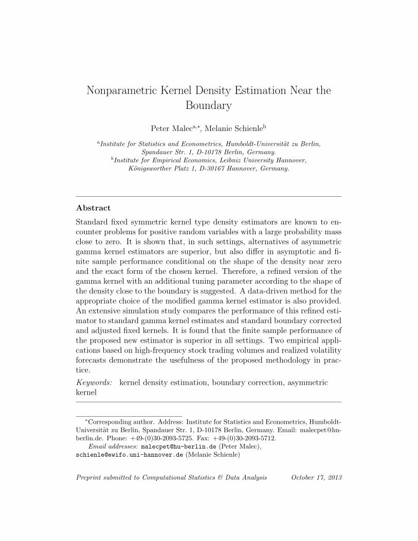
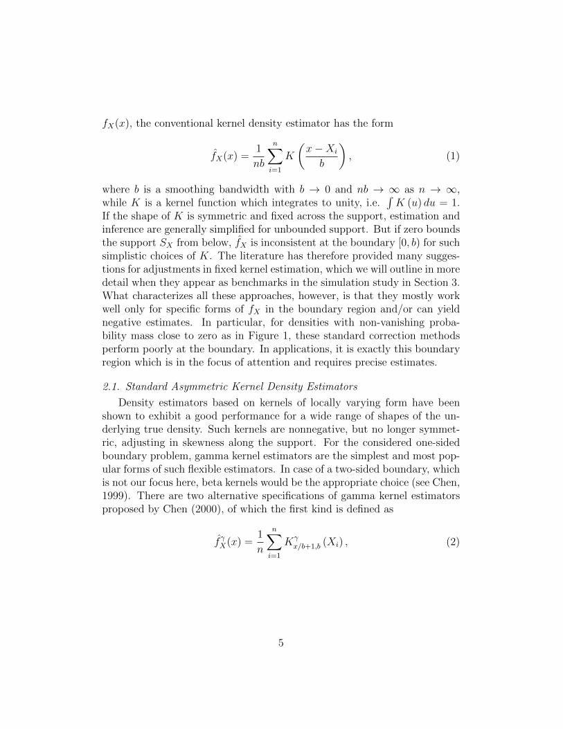
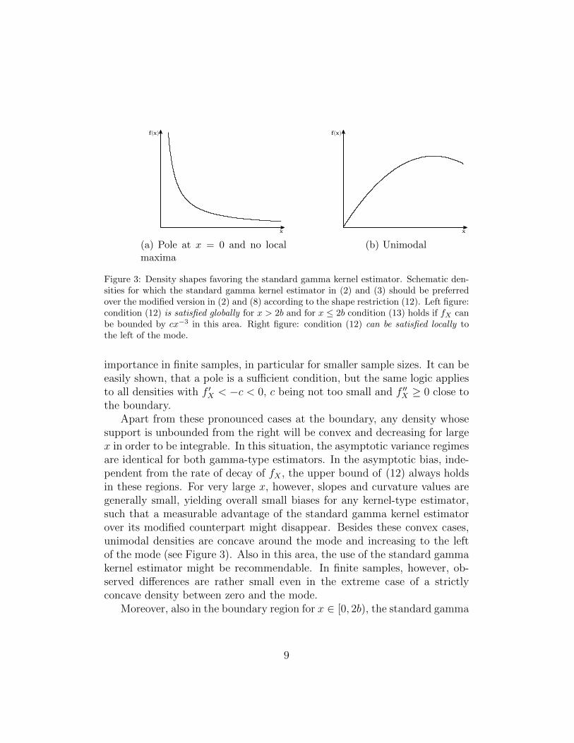
Figure 1: Histograms of intraday trading volumes and realized kernel estimates. We con-sider deseasonalized nonzero 15-Second trading volumes of Citigroup and realized kernelestimates for JP Morgan. Sample period: February 2009 (trading volumes), January 2006– December 2009 (realized kernel). For details on the seasonal adjustment of tradingvolumes and computation of the realized kernel, see Section 4.
and unequal design issues get increasingly severe for higher dimensions, theuse of gamma kernels especially pays off for multivariate density or regressionproblems (see Bouezmarni and Rombouts, 2010a). We also demonstrate thisin a simple multivariate setup as part of our simulation study. The effect be-comes very pronounced and therefore of particular relevance for the extremecase of functional data analysis (see Ferraty and Vieu, 2006; Quintela del Roet al., 2011; Ferraty et al., 2012).
We contribute to the extensive literature on kernel estimation near theboundary by clearly identifying design situations in which finite sample andasymptotic performance of gamma kernel estimates are distinctly superior toany competing fixed kernel adjusted estimates and thus, should be strictlypreferred. Such situations occur when the true f approaches the boundarywith a derivative f ′ significantly different from zero. Such density shapes nat-urally appear in high-frequency data, e.g., when studying aggregated tradingvolumes (see Figure 1), but also in many other applications, such as spectraldensity estimation of long memory time series or when modeling volatilitiesin particular on the intra-daily level (see, e.g., Robinson and Henry, 2003;Corradi et al., 2009).
But we also show that, depending on the underlying shape of the truedensity, the two existing gamma kernel estimators, the so-called standard
3
and modified version as introduced in Chen (2000), might differ substantiallyin boundary performance and still leave significant room for improvement.While in practice almost exclusively a modified gamma-type kernel estimatoris used, we find that, in particular for pole situations, the standard gamma-type estimator yields large performance advantages. We therefore introducea simple data-driven criterion identifying such extreme settings.
For all other design situations, we propose a refined gamma kernel esti-mator, which outperforms all existing estimators in a comprehensive finitesample study. The new estimator introduces a modification parameter ac-cording to the shape of f and its first two derivatives close to the boundary.For determining the appropriate specification of this refined gamma kernelestimator in practice, we also provide an automatic procedure.
Our two applications clearly demonstrate the significant impact of a de-sign dependent choice of gamma-type kernels on the overall estimation re-sults. For high-frequency stock trading volumes, we detect a pole situationand obtain an improved fit from the standard gamma kernel estimator asopposed to the generally applied modified one. In realized variance fore-casts, the new refined gamma kernel estimator is the only one which yieldsresults consistent with financial theory, while all other competing estimatorsproduce an unexpected bias.
2. Kernel Density Estimation at the Boundary
Throughout the paper, we study density estimation for the case that thesupport SX ⊂ R of an unknown density is bounded from one side. Withoutloss of generality, we take this bound to be a lower bound and equal to zero asin many applications like wage distributions, distributions of trading volumes,etc. Obtained results, however, can be easily generalized by appropriatetranslations and reflections at the y-axis. Note also that we restrict ourinitial theoretical exposition to the case of univariate densities for ease ofnotation. Multivariate extensions are then systematically straightforwardvia product kernels. We illustrate this in a simple simulation exercise in amultivariate setting in Section 3, which highlights the gains from using ourmethod in particular for higher dimensions.
For a random sample {Xi}ni=1 from a distribution with unknown density
4
fX(x), the conventional kernel density estimator has the form
fX(x) =1
nb
n∑i=1
K
(x−Xi
b
), (1)
where b is a smoothing bandwidth with b → 0 and nb → ∞ as n → ∞,while K is a kernel function which integrates to unity, i.e.
∫K (u) du = 1.
If the shape of K is symmetric and fixed across the support, estimation andinference are generally simplified for unbounded support. But if zero boundsthe support SX from below, fX is inconsistent at the boundary [0, b) for suchsimplistic choices of K. The literature has therefore provided many sugges-tions for adjustments in fixed kernel estimation, which we will outline in moredetail when they appear as benchmarks in the simulation study in Section 3.What characterizes all these approaches, however, is that they mostly workwell only for specific forms of fX in the boundary region and/or can yieldnegative estimates. In particular, for densities with non-vanishing proba-bility mass close to zero as in Figure 1, these standard correction methodsperform poorly at the boundary. In applications, it is exactly this boundaryregion which is in the focus of attention and requires precise estimates.
2.1. Standard Asymmetric Kernel Density Estimators
Density estimators based on kernels of locally varying form have beenshown to exhibit a good performance for a wide range of shapes of the un-derlying true density. Such kernels are nonnegative, but no longer symmet-ric, adjusting in skewness along the support. For the considered one-sidedboundary problem, gamma kernel estimators are the simplest and most pop-ular forms of such flexible estimators. In case of a two-sided boundary, whichis not our focus here, beta kernels would be the appropriate choice (see Chen,1999). There are two alternative specifications of gamma kernel estimatorsproposed by Chen (2000), of which the first kind is defined as
fγX(x) =1
n
n∑i=1
Kγx/b+1,b (Xi) , (2)
5
where Kγx/b+1,b denotes the density of the gamma distribution with shape
parameter x/b+ 1 and scale parameter b, i.e.
Kγx/b+1,b (u) =
ux/b exp(−u/b)bx/b+1 Γ(x/b+ 1)
. (3)
Consistency and asymptotic normality of the above estimator are straight-forward to derive under standard assumptions. See, e.g., Chen (2000) forthe pointwise and Hagmann and Scaillet (2007) for the uniform version. Fortime series observations, consistency can also be obtained under mixing as-sumptions as in Bouezmarni and Rombouts (2010b). In particular, for asufficiently smooth density fX ∈ C2(SX), it can be shown that bias and vari-ance vanish asymptotically for b→ 0 and nb→∞. Their asymptotic formsare
Bias{fγX(x)
}= b
{f ′X(x) +
1
2xf ′′X(x)
}+ o(b) , (4)
and
Var{fγX(x)
}≈
{fX(x)nbCb(x) if x/b→ κ,
fX(x)2√π
(xb)−1/2 n−1 ifx/b→∞,(5)
where κ is a nonnegative constant and Cb(x) = Γ(2κ+1)21+2κ Γ2(κ+1)
. Accordingly, theasymptotic mean squared error is
MSE{fγX(x)
}≈
{b2{f ′X(x) + 1
2xf ′′X(x)
}2+ fX(x)
nbCb(x) if x/b→ κ,
b2{f ′X(x) + 1
2xf ′′X(x)
}2+ fX(x)
2n√π
(xb)−1/2 ifx/b→∞.(6)
Note that the asymptotic variance decreases for large x, which is offset by anincreasing bias. In contrast to fixed kernel estimators, the asymptotic biascontains the first derivative of the density f ′X , which is due to the fact thatthe chosen flexible kernel shape has its mode rather than its mean at thepoint of estimation x. The modified gamma kernel estimator improves onthis for most of the support without generating convergence problems in theboundary region. In particular, it uses the pdf of a gamma distribution withshape parameter x/b and scale parameter b as kernel function in the interior
6
of the support. This distribution has mean x, but is unbounded for x ap-proaching zero. Therefore, the kernel function consists of two regimes, wherethe boundary form is chosen ad hoc, ensuring a smooth connection to thedesired interior shape, while avoiding unboundedness problems. Accordingto Chen (2000), the estimator is thus defined as
fγmX (x) =1
n
n∑i=1
Kγρb(x),b (Xi) , (7)
where
ρb(x) =
{14
(xb
)2+ 1 if x ∈ [0, 2b) ,
x/b if x ∈ [2b,∞) .(8)
Note that the estimator fixes the size of the boundary region to the areafrom 0 to 2b independent of the shape of the underlying true density. Theasymptotic bias of the modified gamma kernel estimator has the desiredleading term
Bias{fγmX (x)
}=
{ξb(x) bf ′X(x) + o(b) ifx ∈ [0, 2b) ,12xf ′′X(x) b+ o(b) if x ∈ [2b,∞) ,
(9)
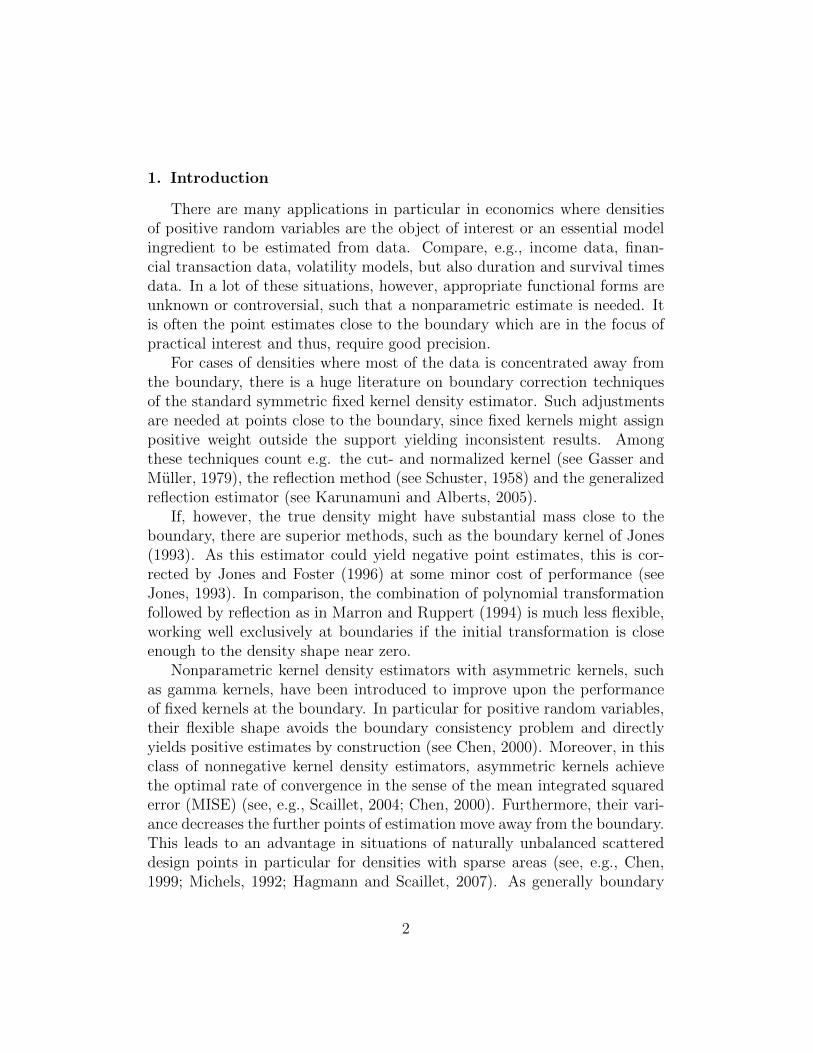
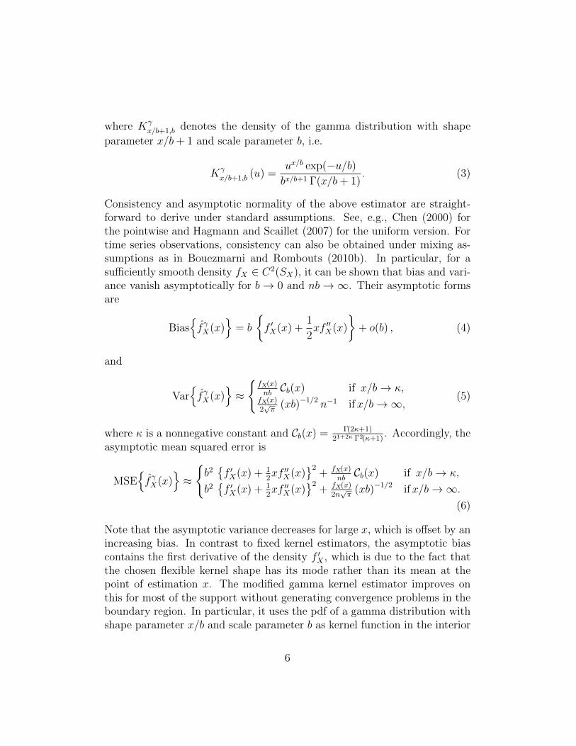
where ξb(x) = (1− x) {ρb(x)− x/b} / {1 + bρb(x)− x}, which is in [0, 1] givenstandard choices of b < 0.5 for all x ∈ [0, 2b) (see Figure 2). Its variancecan be shown to have the same structure as in (5) with modified constant
Cb(x) =Γ(2κ2+1)
21+2κ2 Γ2(κ2+1)and
MSE{fγmX (x)
}≈
{{ξb(x) bf ′X(x)}2 + fX(x)
nbCb(x) if x/b→ κ,{
12xf ′′X(x) b
}2+ fX(x)
2n√π
(xb)−1/2 ifx/b→∞.(10)
See Chen (2000) for details on the derivations.
2.2. Choice of Estimators for Different Density Shapes Near Zero
In general in the literature, the modified gamma kernel estimator has beenstrictly preferred over the standard gamma kernel version. Although a simplecomparison of their asymptotic variances reveals that the constant for themodified estimator, Cb, is strictly larger than its counterpart for the standard
7
(a) b = 0.0091 (b) b = 0.0396
Figure 2: ξb(x). Scale factor ξb(x) = (1− x) {ρb(x)− x/b} / {1 + bρb(x)− x} enteringasymptotic bias and variance of the modified gamma kernel estimator. Bandwidths oftwo DGPs from the simulation study in Section 3 are used.
gamma kernel, Cb, close to the boundary (for all κ < 1), the above choice hasbeen justified by the similarity of the modified gamma kernel to fixed kernelsin terms of asymptotic bias behavior as displayed in (9). However, whencarefully comparing the leading asymptotic bias terms of both gamma-typeestimators, we find that there are cases where it is asymptotically favorableto use the standard gamma kernel estimator. For all x > 2b, in the interiorof the support with
|0.5xf ′′X(x)| > |f ′X(x) + 0.5xf ′′X(x)| , (11)
the standard gamma kernel should be preferred over the modified version.This occurs, in particular, for areas where the density satisfies the shaperestrictions
0 < −f ′X(x)/f ′′X(x) < x . (12)
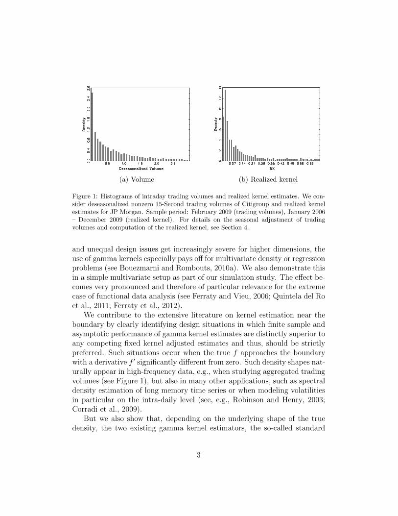
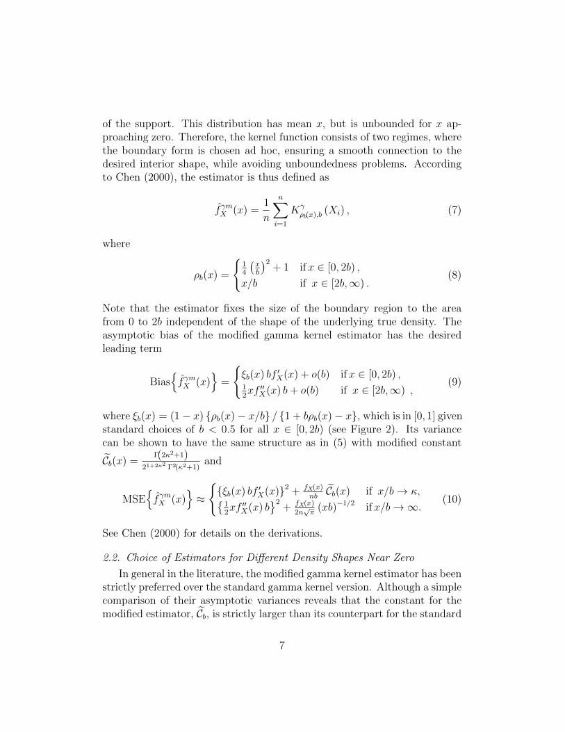
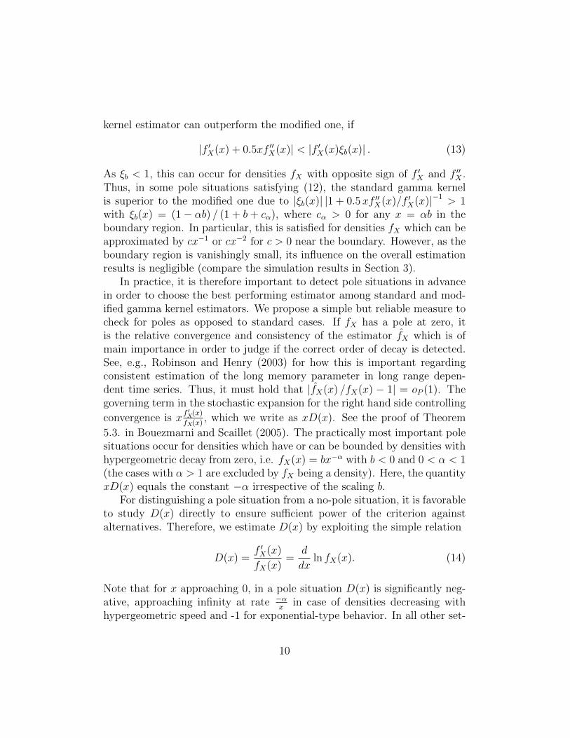
The lower bound is fulfilled for values x where f ′X and f ′′X have differentsigns, i.e. where the density fX is either decreasing and convex or where itis concave and increasing. In the first case, it can be shown that if fX hasa pole at zero, then trivially also the upper bound of (12) is satisfied. Ifadditionally fX does not have any local maxima, the standard gamma kernelshould be preferred over the modified version for the entire interior support(see Figure 3). Our simulation study below confirms that this is also of
8
f(x)
x
(a) Pole at x = 0 and no localmaxima
f(x)
x
(b) Unimodal
Figure 3: Density shapes favoring the standard gamma kernel estimator. Schematic den-sities for which the standard gamma kernel estimator in (2) and (3) should be preferredover the modified version in (2) and (8) according to the shape restriction (12). Left figure:condition (12) is satisfied globally for x > 2b and for x ≤ 2b condition (13) holds if fX canbe bounded by cx−3 in this area. Right figure: condition (12) can be satisfied locally tothe left of the mode.
importance in finite samples, in particular for smaller sample sizes. It can beeasily shown, that a pole is a sufficient condition, but the same logic appliesto all densities with f ′X < −c < 0, c being not too small and f ′′X ≥ 0 close tothe boundary.
Apart from these pronounced cases at the boundary, any density whosesupport is unbounded from the right will be convex and decreasing for largex in order to be integrable. In this situation, the asymptotic variance regimesare identical for both gamma-type estimators. In the asymptotic bias, inde-pendent from the rate of decay of fX , the upper bound of (12) always holdsin these regions. For very large x, however, slopes and curvature values aregenerally small, yielding overall small biases for any kernel-type estimator,such that a measurable advantage of the standard gamma kernel estimatorover its modified counterpart might disappear. Besides these convex cases,unimodal densities are concave around the mode and increasing to the leftof the mode (see Figure 3). Also in this area, the use of the standard gammakernel estimator might be recommendable. In finite samples, however, ob-served differences are rather small even in the extreme case of a strictlyconcave density between zero and the mode.
Moreover, also in the boundary region for x ∈ [0, 2b), the standard gamma
9
kernel estimator can outperform the modified one, if
|f ′X(x) + 0.5xf ′′X(x)| < |f ′X(x)ξb(x)| . (13)
As ξb < 1, this can occur for densities fX with opposite sign of f ′X and f ′′X .Thus, in some pole situations satisfying (12), the standard gamma kernelis superior to the modified one due to |ξb(x)| |1 + 0.5xf ′′X(x)/f ′X(x)|−1 > 1with ξb(x) = (1− αb) / (1 + b+ cα), where cα > 0 for any x = αb in theboundary region. In particular, this is satisfied for densities fX which can beapproximated by cx−1 or cx−2 for c > 0 near the boundary. However, as theboundary region is vanishingly small, its influence on the overall estimationresults is negligible (compare the simulation results in Section 3).
In practice, it is therefore important to detect pole situations in advancein order to choose the best performing estimator among standard and mod-ified gamma kernel estimators. We propose a simple but reliable measure tocheck for poles as opposed to standard cases. If fX has a pole at zero, itis the relative convergence and consistency of the estimator fX which is ofmain importance in order to judge if the correct order of decay is detected.See, e.g., Robinson and Henry (2003) for how this is important regardingconsistent estimation of the long memory parameter in long range depen-dent time series. Thus, it must hold that |fX(x) /fX(x) − 1| = oP (1). Thegoverning term in the stochastic expansion for the right hand side controlling
convergence is xf ′X(x)
fX(x), which we write as xD(x). See the proof of Theorem
5.3. in Bouezmarni and Scaillet (2005). The practically most important polesituations occur for densities which have or can be bounded by densities withhypergeometric decay from zero, i.e. fX(x) = bx−α with b < 0 and 0 < α < 1(the cases with α > 1 are excluded by fX being a density). Here, the quantityxD(x) equals the constant −α irrespective of the scaling b.
For distinguishing a pole situation from a no-pole situation, it is favorableto study D(x) directly to ensure sufficient power of the criterion againstalternatives. Therefore, we estimate D(x) by exploiting the simple relation
D(x) =f ′X(x)
fX(x)=
d
dxln fX(x). (14)
Note that for x approaching 0, in a pole situation D(x) is significantly neg-ative, approaching infinity at rate −α
xin case of densities decreasing with
hypergeometric speed and -1 for exponential-type behavior. In all other set-
10
tings where the modified gamma kernel is the method of choice, D(x) issignificantly positive. As a criterion, D(x) combines properties of the den-sity and its slope to distinguish the pole situation from other density shapes.This is more powerful than checking density and slope separately in isola-tion. In practice, D(x) can be estimated by the difference quotient based onmodified gamma kernels
D(x) =ln fγmX (x+ b)− ln fγmX (x)
b, (15)
where b > 0 is the same bandwidth as for the density estimates at x andx + b. For the practical scope of this paper, it is sufficient to work witha rough criterion checking if D(x) is significantly negative or not. Devel-oping a novel formal test for the H0 of a hypergeometric pole situation isbeyond the scope of this paper. We conjecture that, using the results in Fer-nandes and Grammig (2005) for specification testing in the simple densitycase, the corresponding asymptotic distribution of the centered test statistic
nb2(D(x) + α
x
)could be derived. However, as calculations are quite involved
and should be complemented with a valid bootstrap approximation schemefor finite samples, we leave this for future research and a paper on its own.
2.3. Refined Estimation with Modified Gamma Kernels
In cases where we can exclude a pole at the boundary, the modifiedgamma kernel generally should be the method of choice in terms of bestasymptotic performance. In the literature, its chosen form in particular inthe boundary region has mainly been justified by (computational) conve-nience. However, our simulation results clearly indicate that alternative flex-ible specifications can significantly improve upon the performance of standardmodified gamma kernels.
In particular, we propose simple refined versions of the modified gammakernel, including an additional specification parameter c that allows forhigher accuracy if appropriately chosen in a data-driven way. We studytwo types of refined modified gamma kernels, i.e.
11
ρvIb (x) =
[
14
(xbc
)2+ 1]
[c+ 2b (1− c)] ifx ∈ [0, 2bc) ,
xbc
(c+ 2b− x) if x ∈ [2bc, 2b) ,
x/b if x ∈ [2b,∞) ,
(16)
and
ρvIIb (x) =
{14
(xbc
)2+ 1 if x ∈ [0, 2bc) ,
x/(bc) if x ∈ [2bc,∞) ,(17)
where c ∈ (0, 1] with c = 1 yielding the original parameterization in bothcases. Specification vI shifts the boundary regime below one and introducesa flexible quadratic middle part. In the latter regime, for ρb(x) > x/b wehave that x/b < ρvIb (x) < ρb(x) if
x
b
2b− xρb(x)− x/b
< c < 1, x ∈ [2bc, 2b) , (18)
where ρb(x) is defined as in (8). Importantly, fulfillment of the conditionimplies that specification vI is closer to the theoretically optimal situationwith the mean of the kernel being at the observation point as compared tothe original modified gamma kernel. The second alternative, vII, keeps tworegimes and the general structure of the original specification, but shrinksthe boundary region proportionally to the value of the tuning parameter c.This modification also affects asymptotics in the interior of the support, asthe mean of the kernel equals x/c and hence, only in the trivial case c = 1coincides with the point of estimation.
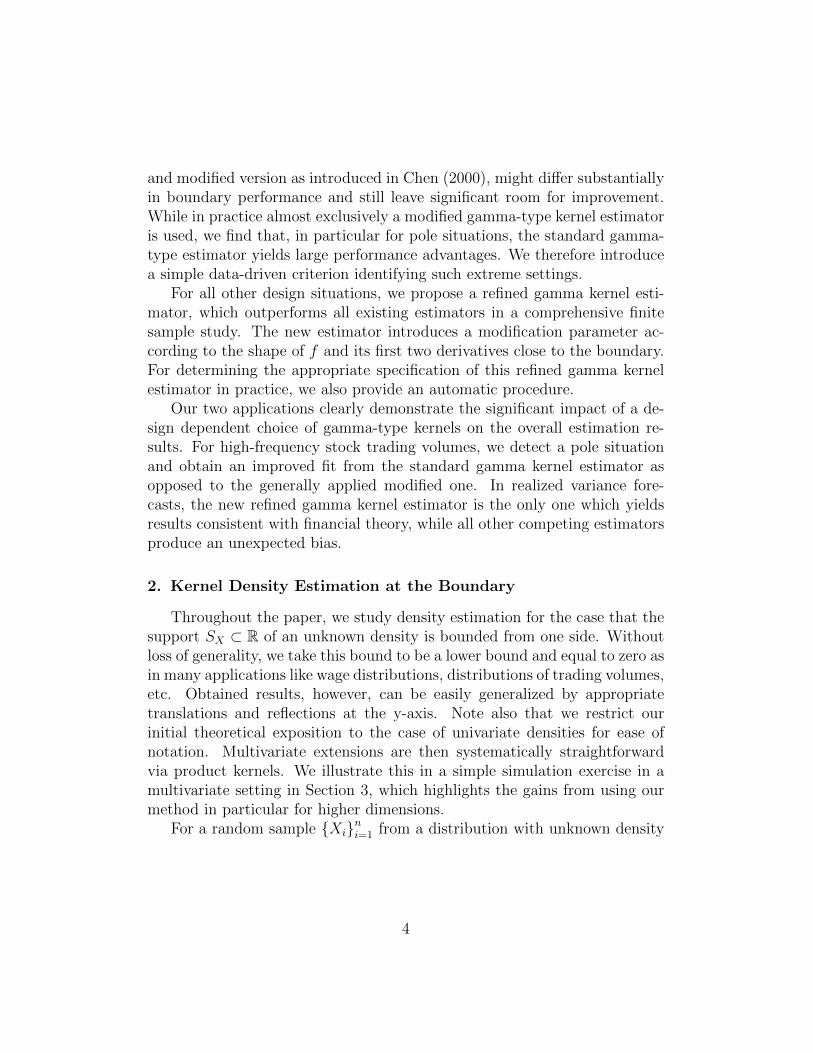
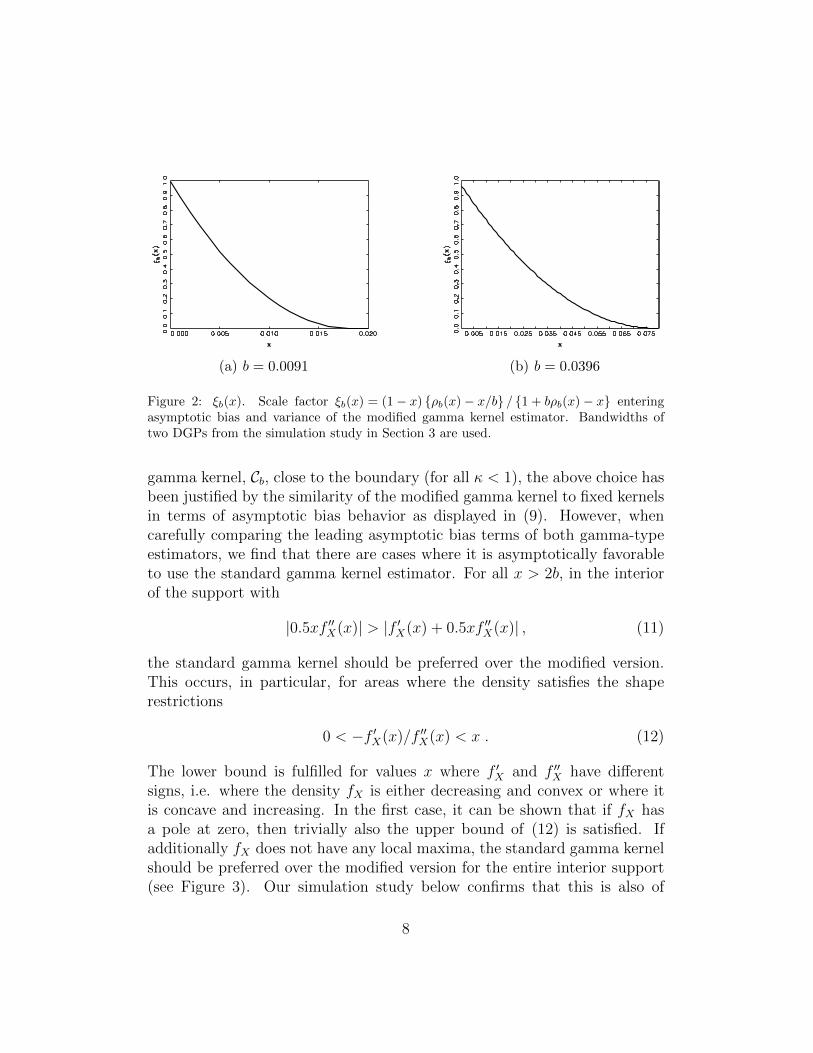
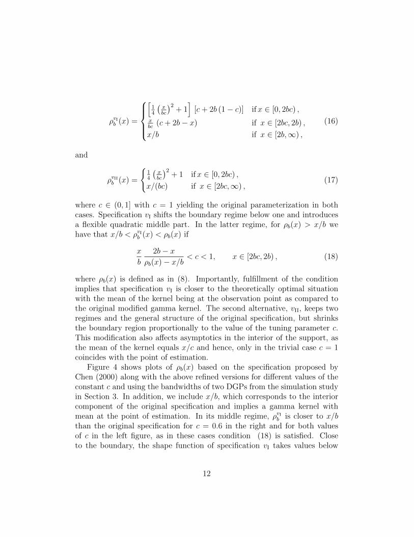
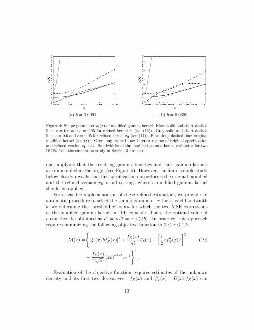
Figure 4 shows plots of ρb(x) based on the specification proposed byChen (2000) along with the above refined versions for different values of theconstant c and using the bandwidths of two DGPs from the simulation studyin Section 3. In addition, we include x/b, which corresponds to the interiorcomponent of the original specification and implies a gamma kernel withmean at the point of estimation. In its middle regime, ρvIb is closer to x/bthan the original specification for c = 0.6 in the right and for both valuesof c in the left figure, as in these cases condition (18) is satisfied. Closeto the boundary, the shape function of specification vI takes values below
12
(a) b = 0.0091 (b) b = 0.0396
Figure 4: Shape parameter ρb(x) of modified gamma kernel. Black solid and short-dashedline: c = 0.6 and c = 0.05 for refined kernel vI (see (16)). Grey solid and short-dashedline: c = 0.6 and c = 0.05 for refined kernel vII (see (17)). Black long-dashed line: originalmodified kernel (see (8)). Grey long-dashed line: interior regime of original specificationand refined version vI, x/b. Bandwidths of the modified gamma kernel estimator for twoDGPs from the simulation study in Section 3 are used.
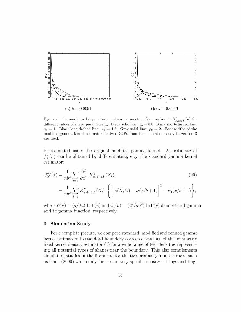
one, implying that the resulting gamma densities and thus, gamma kernelsare unbounded at the origin (see Figure 5). However, the finite sample studybelow clearly reveals that this specification outperforms the original modifiedand the refined version vII in all settings where a modified gamma kernelshould be applied.
For a feasible implementation of these refined estimators, we provide anautomatic procedure to select the tuning parameter c: for a fixed bandwidthb, we determine the threshold xc = b κ for which the two MSE expressionsof the modified gamma kernel in (10) coincide. Then, the optimal value ofc can then be obtained as c∗ = κ/2 = xc/ (2 b). In practice, this approachrequires minimizing the following objective function in 0 ≤ x ≤ 2 b:
M(x) =
{[ξb(x) bf ′X(x)]
2+fX(x)
nbCb(x)−
[1
2xf ′′X(x) b
]2
(19)
− fX(x)
2√π
(xb)−1/2 n−1
}2
.
Evaluation of the objective function requires estimates of the unknowndensity and its first two derivatives. fX(x) and f ′X(x) = D(x) fX(x) can
different values of shape parameter ρb. Black solid line: ρb = 0.5. Black short-dashed line:ρb = 1. Black long-dashed line: ρb = 1.5. Grey solid line: ρb = 2. Bandwidths of themodified gamma kernel estimator for two DGPs from the simulation study in Section 3are used.
be estimated using the original modified gamma kernel. An estimate off ′′X(x) can be obtained by differentiating, e.g., the standard gamma kernelestimator:
f ′′γX (x) =1
nb2
n∑i=1
∂2
∂x2Kγx/b+1,b (Xi) , (20)
=1
nb2
n∑i=1
Kγx/b+1,b (Xi)
{[ln(Xi/b)− ψ(x/b+ 1)
]2
− ψ1(x/b+ 1)
},
where ψ(u) = (d/du) ln Γ(u) and ψ1(u) = (d2/du2) ln Γ(u) denote the digammaand trigamma function, respectively.
3. Simulation Study
For a complete picture, we compare standard, modified and refined gammakernel estimators to standard boundary corrected versions of the symmetricfixed kernel density estimator (1) for a wide range of test densities represent-ing all potential types of shapes near the boundary. This also complementssimulation studies in the literature for the two original gamma kernels, suchas Chen (2000) which only focuses on very specific density settings and Hag-
14
mann and Scaillet (2007) which is restrictive in the range of fixed boundarykernel competitors.
All fixed kernels are based on the Epanechnikov kernel K(u) = 3/4(1 −u2)1I(−1 ≤ u ≤ 1), where 1I(·) denotes an indicator function limiting the sup-port of K to [−1, 1]. In particular, we report results for the following fivecompeting fixed kernel adjustments.
The reflection estimator proposed by Schuster (1958) has the form
fReflX (x) =
1
nb
∑i=1
[K
(x−Xi
b
)+K
(x+Xi
b
)]. (21)
In the inside of the support for x ≥ 2h, it coincides with the standard kerneldensity estimator fFixed
X in (1).Karunamuni and Alberts (2005) generalize the reflection estimator (21)
to
fGReflX (x) =
1
nb
∑i=1
[K
(x− gν(Xi)
b
)+K
(x+ gν(Xi)
b
)], (22)
where gν(y) = y + (1/2) d0 k′ν y
2 + λ0
(d0 k
′ν
)2
y3, with d0 being an estimate
of d0 := f ′X(0) /fX(0) and
k′ν = 2
∫ 1
ν
(u− ν)K (u) du
/(ν + 2
∫ 1
ν
(u− ν)K (u) du
), ν := x/b, (23)
while λ0 is a constant such that 12λ0 > 1. We estimate d0 as outlined inSection 2.2 and 3 of Karunamuni and Alberts (2005).
In the cut-and-normalized estimator fCaNX introduced by Gasser and Muller
(1979), the kernel function K for the boundary region is truncated at ν andnormalized, ensuring integration to unity. For the Epanechnikov kernel, ithas the form
KCaN (u) =(1− u2)∫ ν
−1(1− u2) du
1I{−1≤u≤ν} . (24)
General boundary corrected estimators fBoundX (see, e.g., Jones, 1993) re-
place the standard kernel function in the boundary region by a modified
15
version KBound, which is chosen to meet the following conditions:∫ 1
ν
KBound (u) du = 0,
∫ ν
−1
KBound (u) du <∞,∫ ν
−1
KBound (u)u du = 0.
(25)
We use the boundary kernel based on the Epanechnikov kernel, which hasthe following form:
KBound (u) = 12(1 + u)
(1 + ν)4
[3ν2 − 2ν + 1
2+ u (1− 2u)
]1I{−1≤u≤ν}. (26)
A method that corrects for the possible negativity of the boundary kernelestimates was proposed, e.g., by Jones and Foster (1996). The estimator hasthe following form:
fJFX (x) = fCaN
X (x) exp
{fBoundX (x)
fCaNX (x)
− 1
}. (27)
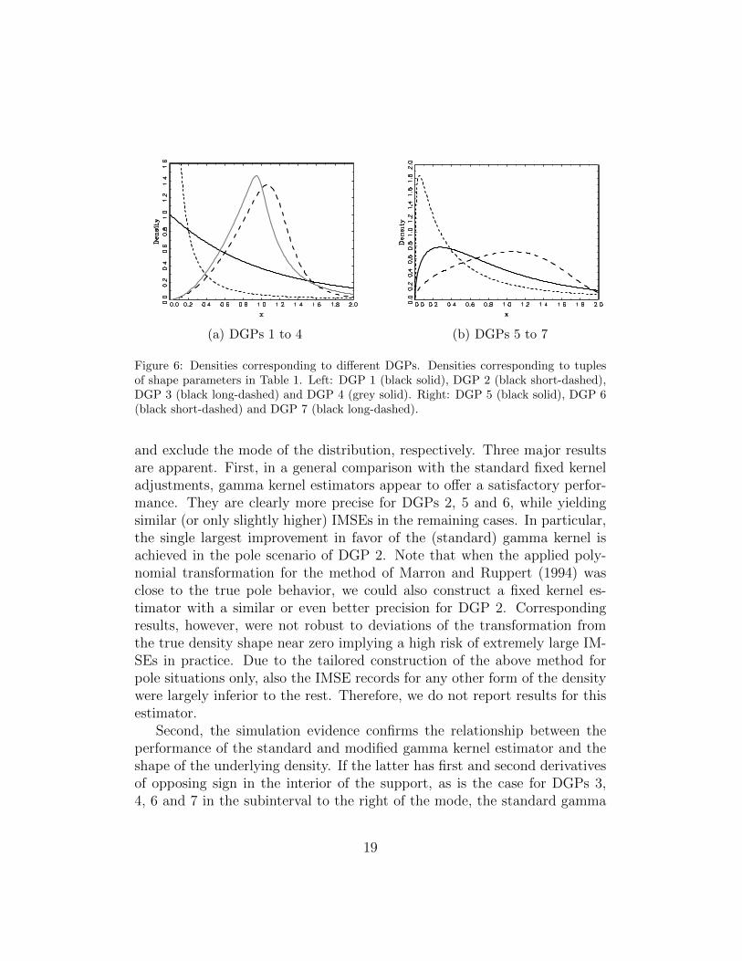
We compare the performance of the estimators for seven different densityfunctions with nonnegative support, which reflect the variety of practicallyrelevant types of shapes on left-bounded support. The densities of DGP 1and DGP 2 are entirely decreasing and convex with DGP 2 exhibiting polebehavior at zero. The remaining densities are increasing near the bound-ary. For DGP 3 and 4, the density is locally convex in the boundary region,while for 5,6 and 7 it is concave with varying degree of steepness. The cor-responding density shapes are depicted in Figure 6. All DGPs are generatedfrom different specifications of the flexible generalized F distribution, whichis based on a gamma mixture of the generalized gamma distribution (see,e.g., Lancaster, 1997). Its marginal density function is given by
fx(x) =a xam−1 [η + (x/λ)a]
(−η−m)ηη
λam B(m, η), (28)
where a > 0,m > 0, η > 0 and λ > 0. B(·) describes the full Beta function
with B(m, η) := Γ(m)Γ(η)Γ(m+η)
. Table 1 shows the values of the shape parametersa, m and η for the seven DGPs considered. To ensure comparability acrossthe different DGPs, the expectation is restricted to one by setting the scale
16
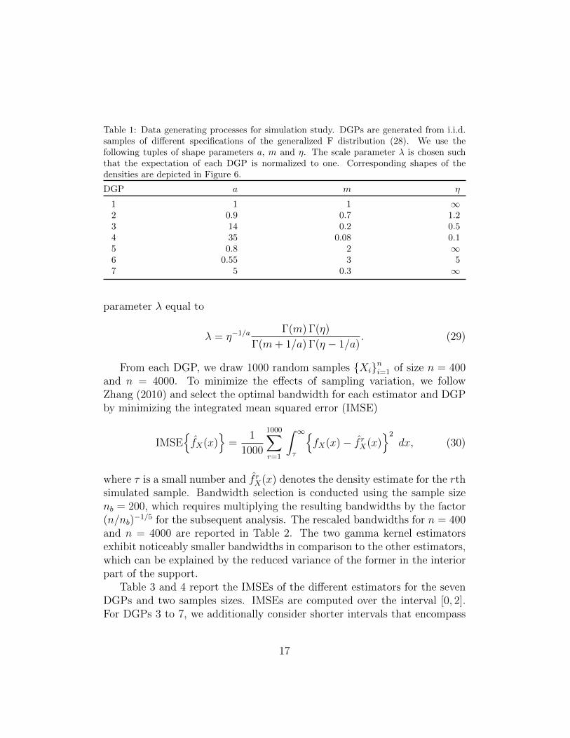
Table 1: Data generating processes for simulation study. DGPs are generated from i.i.d.samples of different specifications of the generalized F distribution (28). We use thefollowing tuples of shape parameters a, m and η. The scale parameter λ is chosen suchthat the expectation of each DGP is normalized to one. Corresponding shapes of thedensities are depicted in Figure 6.
From each DGP, we draw 1000 random samples {Xi}ni=1 of size n = 400and n = 4000. To minimize the effects of sampling variation, we followZhang (2010) and select the optimal bandwidth for each estimator and DGPby minimizing the integrated mean squared error (IMSE)
IMSE{fX(x)
}=
1
1000
1000∑r=1
∫ ∞τ
{fX(x)− f rX(x)
}2
dx, (30)
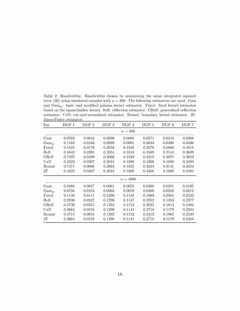
where τ is a small number and f rX(x) denotes the density estimate for the rthsimulated sample. Bandwidth selection is conducted using the sample sizenb = 200, which requires multiplying the resulting bandwidths by the factor(n/nb)
−1/5 for the subsequent analysis. The rescaled bandwidths for n = 400and n = 4000 are reported in Table 2. The two gamma kernel estimatorsexhibit noticeably smaller bandwidths in comparison to the other estimators,which can be explained by the reduced variance of the former in the interiorpart of the support.
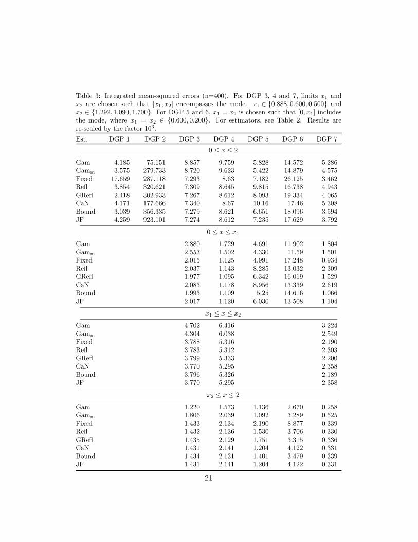
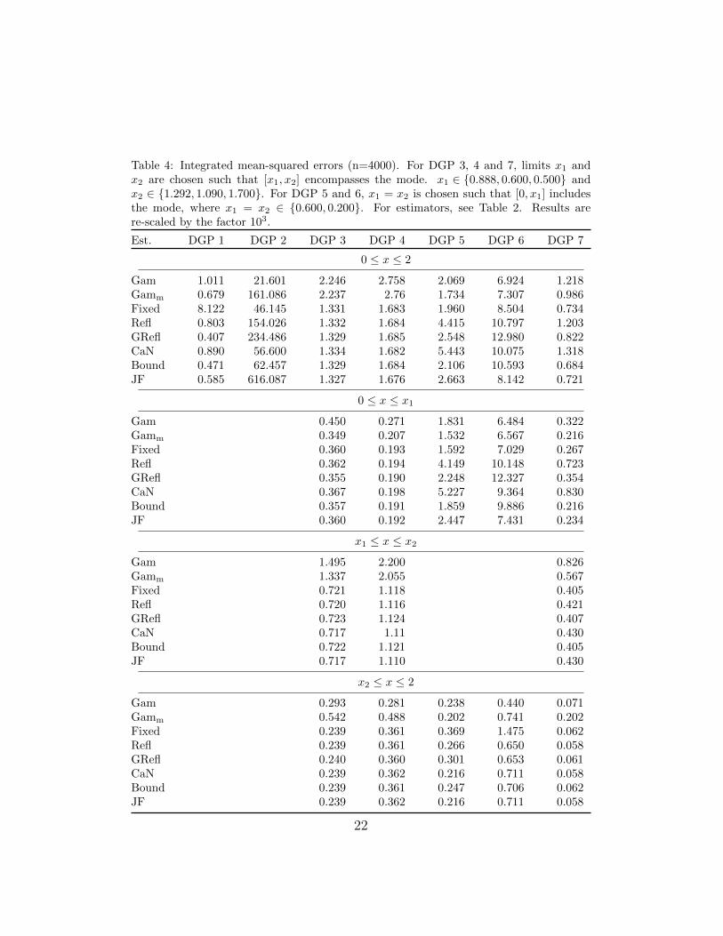
Table 3 and 4 report the IMSEs of the different estimators for the sevenDGPs and two samples sizes. IMSEs are computed over the interval [0, 2].For DGPs 3 to 7, we additionally consider shorter intervals that encompass
17
Table 2: Bandwidths. Bandwidths chosen by minimizing the mean integrated squarederror (30) using simulated samples with n = 200. The following estimators are used. Gamand Gamm: basic and modified gamma kernel estimator. Fixed: fixed kernel estimatorbased on the epanechnikov kernel. Refl: reflection estimator. GRefl: generalized reflectionestimator. CaN: cut-and-normalized estimator. Bound: boundary kernel estimator. JF:Jones-Foster estimator.
Figure 6: Densities corresponding to different DGPs. Densities corresponding to tuplesof shape parameters in Table 1. Left: DGP 1 (black solid), DGP 2 (black short-dashed),DGP 3 (black long-dashed) and DGP 4 (grey solid). Right: DGP 5 (black solid), DGP 6(black short-dashed) and DGP 7 (black long-dashed).
and exclude the mode of the distribution, respectively. Three major resultsare apparent. First, in a general comparison with the standard fixed kerneladjustments, gamma kernel estimators appear to offer a satisfactory perfor-mance. They are clearly more precise for DGPs 2, 5 and 6, while yieldingsimilar (or only slightly higher) IMSEs in the remaining cases. In particular,the single largest improvement in favor of the (standard) gamma kernel isachieved in the pole scenario of DGP 2. Note that when the applied poly-nomial transformation for the method of Marron and Ruppert (1994) wasclose to the true pole behavior, we could also construct a fixed kernel es-timator with a similar or even better precision for DGP 2. Correspondingresults, however, were not robust to deviations of the transformation fromthe true density shape near zero implying a high risk of extremely large IM-SEs in practice. Due to the tailored construction of the above method forpole situations only, also the IMSE records for any other form of the densitywere largely inferior to the rest. Therefore, we do not report results for thisestimator.
Second, the simulation evidence confirms the relationship between theperformance of the standard and modified gamma kernel estimator and theshape of the underlying density. If the latter has first and second derivativesof opposing sign in the interior of the support, as is the case for DGPs 3,4, 6 and 7 in the subinterval to the right of the mode, the standard gamma
19
kernel yields noticeably lower IMSEs (see bottom panel). When consideringthe entire interval [0, 2], the standard gamma kernel is more precise for DGPs2 and 6 with the most striking gains occurring in the former scenario, as itcorresponds to a globally convex density with pole at zero. Finally, the aboverelation breaks down within the boundary region due to the involvement ofthe factor ξb(x) in the asymptotic bias (see (9)). For DGPs 5 and 6, themodified gamma kernel implies lower IMSEs over the leftmost subinterval inwhich the corresponding densities are increasing and concave (see lower toppanel).
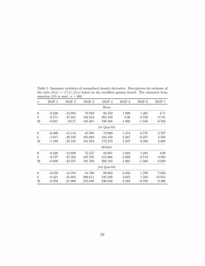
The simulation results stress the importance of determining pole situa-tions in advance, which can be achieved by examining the normalized densityderivative D(x) in the boundary region. We estimate the latter as in (15)using the modified gamma kernel for the points x ∈ {0, b, 2b}, where b isthe bandwidth of the corresponding estimator. Table 5 reports descriptivestatistics of the estimates for n = 400. In case of DGP 2, these estimates arehighly negative at all three points, demonstrating that our simple methodis able to detect a pole at zero. We obtain negative estimates at all or atdistinct points also for DGPs 1 and 6, but their magnitude is considerablylower than in the above true pole scenario.
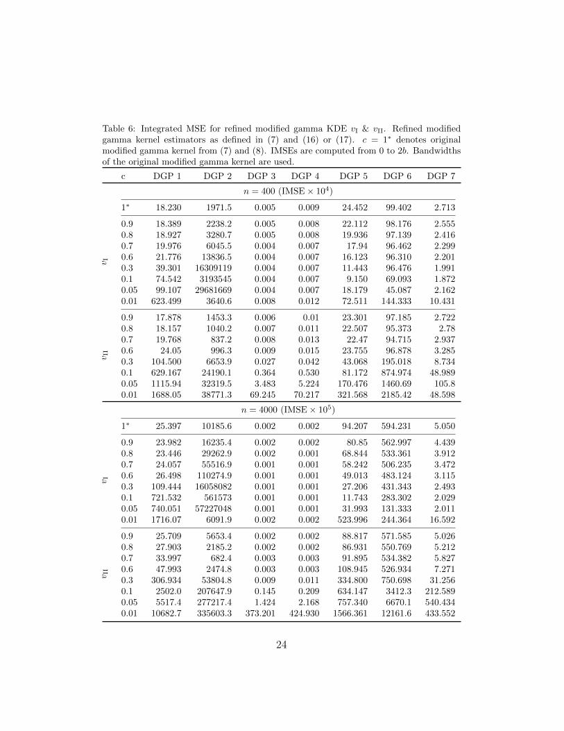
As was argued in Section 2.2, whenever no pole situation has been de-tected, the modified gamma kernel in its original or refined form should beused. The IMSEs of the three corresponding estimators are displayed inTable 6. For the refined kernels vI and vII, a set of values for the thresh-old c is considered. To ensure comparability, we apply the bandwidths b ofthe original modified gamma kernel to all estimators and also use 2b as theupper integration limit in the IMSE calculations. The main finding is thatthe refined kernel vI exhibits a high precision in all situations for which themodified kernel should be considered, i.e. all DGPs except the second one.The improvement with respect to the original specification is particularlypronounced, accompanied by low optimal values of the constant c, in caseof densities with concave shape near the boundary, as in DGPs 5,6 and 7.Further, the refined kernel vII is at roughly the same level as the traditionalparameterization and even yields the lowest IMSE for DGP 1 when n = 400.However, recall that this specification makes the boundary region smallerand has neither its mean nor mode at the point of estimation for x > 2bc(see Section 2.3). These properties cause a vastly lower precision comparedto the other specifications in the interior part of the support. Correspondingsimulation results are available upon request.
20
Table 3: Integrated mean-squared errors (n=400). For DGP 3, 4 and 7, limits x1 andx2 are chosen such that [x1, x2] encompasses the mode. x1 ∈ {0.888, 0.600, 0.500} andx2 ∈ {1.292, 1.090, 1.700}. For DGP 5 and 6, x1 = x2 is chosen such that [0, x1] includesthe mode, where x1 = x2 ∈ {0.600, 0.200}. For estimators, see Table 2. Results arere-scaled by the factor 103.
Table 4: Integrated mean-squared errors (n=4000). For DGP 3, 4 and 7, limits x1 andx2 are chosen such that [x1, x2] encompasses the mode. x1 ∈ {0.888, 0.600, 0.500} andx2 ∈ {1.292, 1.090, 1.700}. For DGP 5 and 6, x1 = x2 is chosen such that [0, x1] includesthe mode, where x1 = x2 ∈ {0.600, 0.200}. For estimators, see Table 2. Results arere-scaled by the factor 103.
Table 5: Summary statistics of normalized density derivative. Descriptives for estimate ofthe ratio D(x) := f ′(x) /f(x) based on the modified gamma kernel. The estimator fromequation (15) is used. n = 400.
Table 6: Integrated MSE for refined modified gamma KDE vI & vII. Refined modifiedgamma kernel estimators as defined in (7) and (16) or (17). c = 1∗ denotes originalmodified gamma kernel from (7) and (8). IMSEs are computed from 0 to 2b. Bandwidthsof the original modified gamma kernel are used.
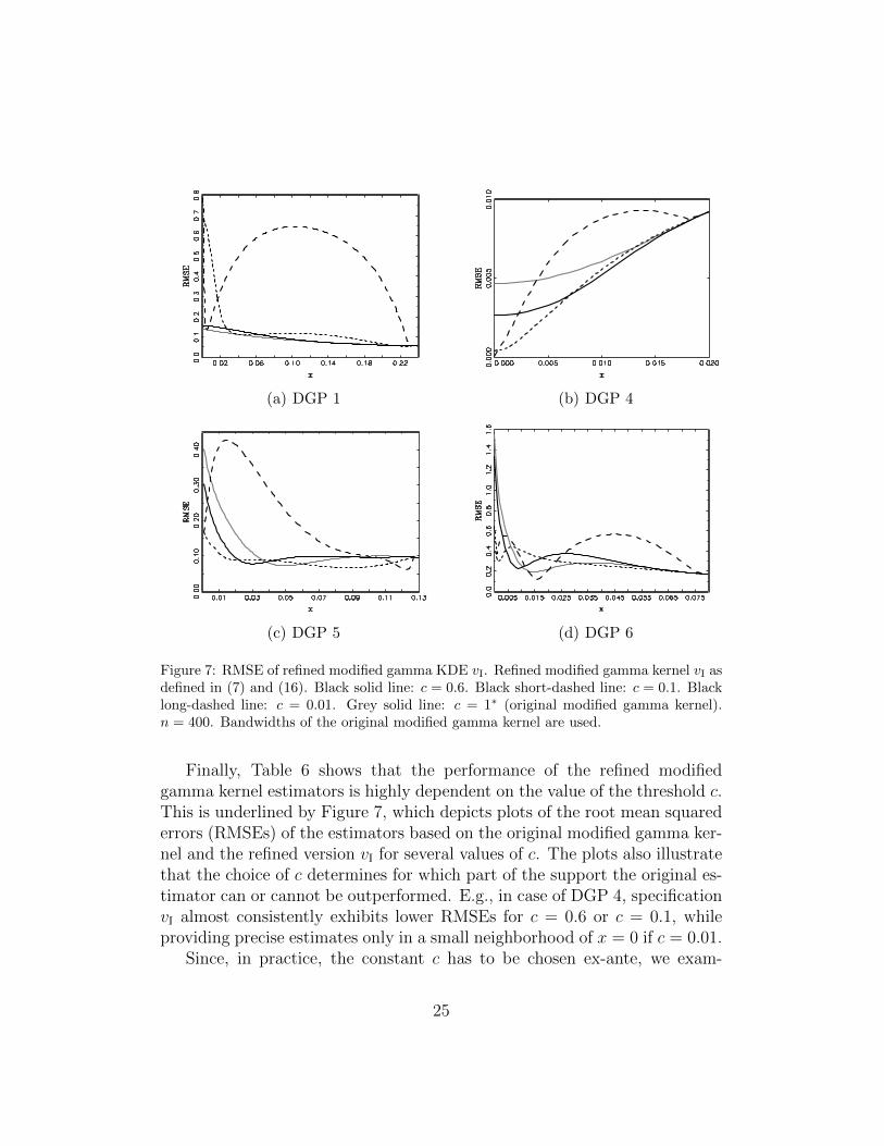
Figure 7: RMSE of refined modified gamma KDE vI. Refined modified gamma kernel vI asdefined in (7) and (16). Black solid line: c = 0.6. Black short-dashed line: c = 0.1. Blacklong-dashed line: c = 0.01. Grey solid line: c = 1∗ (original modified gamma kernel).n = 400. Bandwidths of the original modified gamma kernel are used.
Finally, Table 6 shows that the performance of the refined modifiedgamma kernel estimators is highly dependent on the value of the threshold c.This is underlined by Figure 7, which depicts plots of the root mean squarederrors (RMSEs) of the estimators based on the original modified gamma ker-nel and the refined version vI for several values of c. The plots also illustratethat the choice of c determines for which part of the support the original es-timator can or cannot be outperformed. E.g., in case of DGP 4, specificationvI almost consistently exhibits lower RMSEs for c = 0.6 or c = 0.1, whileproviding precise estimates only in a small neighborhood of x = 0 if c = 0.01.
Since, in practice, the constant c has to be chosen ex-ante, we exam-
25
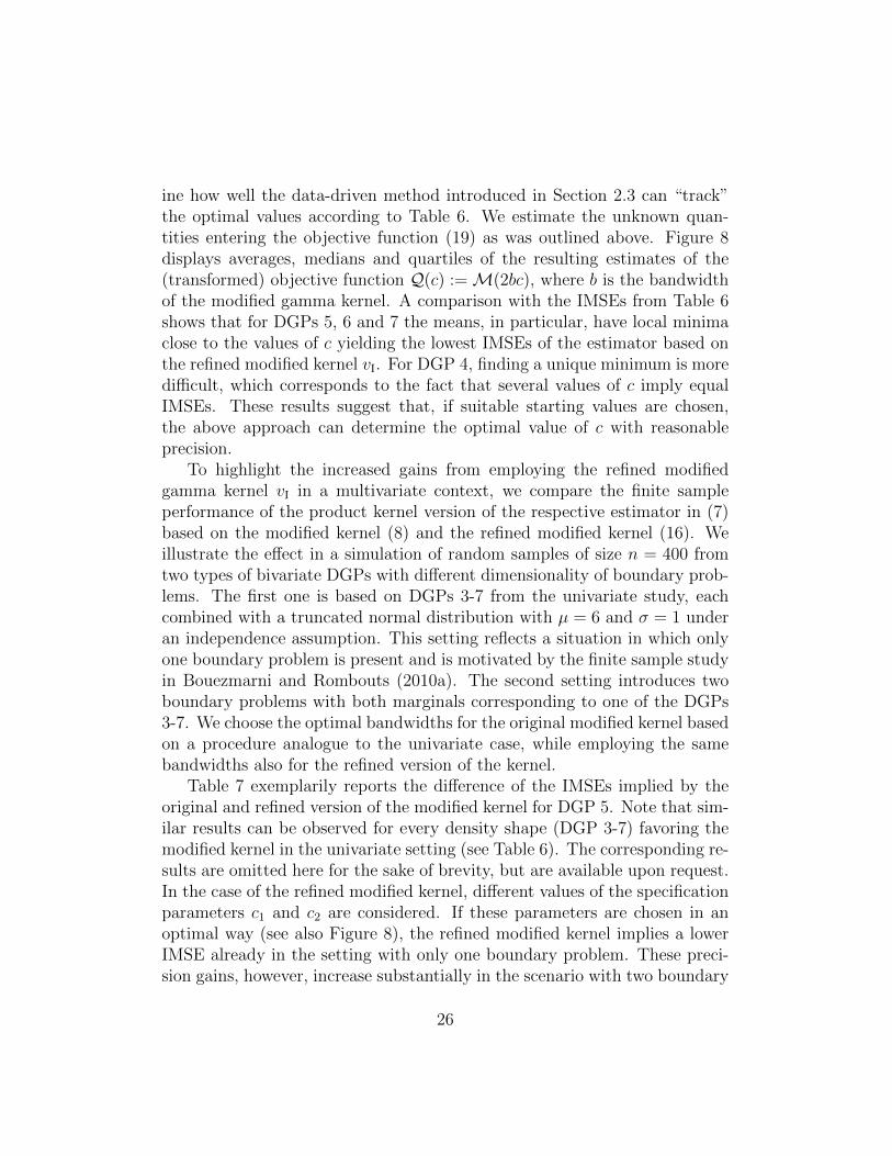
ine how well the data-driven method introduced in Section 2.3 can “track”the optimal values according to Table 6. We estimate the unknown quan-tities entering the objective function (19) as was outlined above. Figure 8displays averages, medians and quartiles of the resulting estimates of the(transformed) objective function Q(c) :=M(2bc), where b is the bandwidthof the modified gamma kernel. A comparison with the IMSEs from Table 6shows that for DGPs 5, 6 and 7 the means, in particular, have local minimaclose to the values of c yielding the lowest IMSEs of the estimator based onthe refined modified kernel vI. For DGP 4, finding a unique minimum is moredifficult, which corresponds to the fact that several values of c imply equalIMSEs. These results suggest that, if suitable starting values are chosen,the above approach can determine the optimal value of c with reasonableprecision.
To highlight the increased gains from employing the refined modifiedgamma kernel vI in a multivariate context, we compare the finite sampleperformance of the product kernel version of the respective estimator in (7)based on the modified kernel (8) and the refined modified kernel (16). Weillustrate the effect in a simulation of random samples of size n = 400 fromtwo types of bivariate DGPs with different dimensionality of boundary prob-lems. The first one is based on DGPs 3-7 from the univariate study, eachcombined with a truncated normal distribution with µ = 6 and σ = 1 underan independence assumption. This setting reflects a situation in which onlyone boundary problem is present and is motivated by the finite sample studyin Bouezmarni and Rombouts (2010a). The second setting introduces twoboundary problems with both marginals corresponding to one of the DGPs3-7. We choose the optimal bandwidths for the original modified kernel basedon a procedure analogue to the univariate case, while employing the samebandwidths also for the refined version of the kernel.
Table 7 exemplarily reports the difference of the IMSEs implied by theoriginal and refined version of the modified kernel for DGP 5. Note that sim-ilar results can be observed for every density shape (DGP 3-7) favoring themodified kernel in the univariate setting (see Table 6). The corresponding re-sults are omitted here for the sake of brevity, but are available upon request.In the case of the refined modified kernel, different values of the specificationparameters c1 and c2 are considered. If these parameters are chosen in anoptimal way (see also Figure 8), the refined modified kernel implies a lowerIMSE already in the setting with only one boundary problem. These preci-sion gains, however, increase substantially in the scenario with two boundary
26
(a) DGP 4 (b) DGP 5
(c) DGP 6 (d) DGP 7
Figure 8: Objective function for choice of c. Mean (black solid), median (grey solid), first(black long-dashed) and third (black short-dashed) quartile of (transformed) objectivefunction for choice of the constant c in the refined modified gamma kernel vI as defined in(7) and (16). The transformed objective function is Q(c) :=M(2bc), whereM(x) is givenin (19) and b denotes the bandwidth of the original modified gamma kernel. n = 400.
27
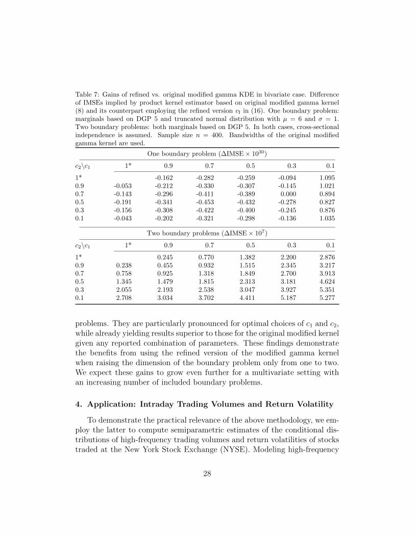
Table 7: Gains of refined vs. original modified gamma KDE in bivariate case. Differenceof IMSEs implied by product kernel estimator based on original modified gamma kernel(8) and its counterpart employing the refined version vI in (16). One boundary problem:marginals based on DGP 5 and truncated normal distribution with µ = 6 and σ = 1.Two boundary problems: both marginals based on DGP 5. In both cases, cross-sectionalindependence is assumed. Sample size n = 400. Bandwidths of the original modifiedgamma kernel are used.
problems. They are particularly pronounced for optimal choices of c1 and c2,while already yielding results superior to those for the original modified kernelgiven any reported combination of parameters. These findings demonstratethe benefits from using the refined version of the modified gamma kernelwhen raising the dimension of the boundary problem only from one to two.We expect these gains to grow even further for a multivariate setting withan increasing number of included boundary problems.
4. Application: Intraday Trading Volumes and Return Volatility
To demonstrate the practical relevance of the above methodology, we em-ploy the latter to compute semiparametric estimates of the conditional dis-tributions of high-frequency trading volumes and return volatilities of stockstraded at the New York Stock Exchange (NYSE). Modeling high-frequency
28
trading volumes is, for instance, relevant for trading strategies replicating the(daily) volume weighted average price (VWAP). Estimates of conditionalvolatility distributions are crucial for the pricing of volatility derivatives.Examples include options and futures on the CBOE Volatility Index (VIX)trading at the Chicago Board Options Exchange (CBOE).
4.1. Modeling Intraday Trading Volumes
We consider transaction data for Citigroup from the last trading weekof February 2009. The raw sample is filtered by deleting transactions thatoccurred outside regular trading hours from 9:30 am to 4:00 pm, computingcumulated trading volumes over 15 second intervals and removing zero ob-servations, which yields a sample size of 7452. For a detailed discussion ofthe treatment of zero observations in the context of financial high-frequencydata, see Hautsch et al. (2013). To capture the well-known intraday sea-sonalities of high-frequency trading variables (see, e.g., Hautsch (2004) foran overview), we divide the cumulated volumes by a seasonality componentwhich is pre-estimated employing a cubic spline function.
An important property of the resulting (deseasonalized) trading volumesis the strong persistence, as evidenced by the highly significant Ljung-Boxstatistics in Table 8. The most widely-used parametric framework for thistype of data, see, e.g., Brownlees et al. (2010), is the multiplicative errormodel (MEM) originally proposed by Engle (2002). Accordingly, we decom-
pose the t-th trading volume, x(v)t , as
x(v)t = µ
(v)t ε
(v)t , ε
(v)t ∼ i.i.d. D(1) , (31)
where µ(v)t denotes the conditional mean given the past information set F (v)
t−1
and is assumed to evolve according to the dynamics described in AppendixA.ε
(v)t is a disturbance following an unspecified distribution D(1) with positive
support and E[ε
(v)t
]= 1. Assuming MEM-type dynamics would allow to ap-
ply gamma kernel estimators to trading volumes directly and estimate theirunconditional density fX
(x
(v)t
)consistently (see Bouezmarni and Rombouts,
2010b). Our object of interest, the conditional density given the past infor-
mation set F (v)t−1, can be estimated semiparametrically in a straightforward
way, as the MEM structure implies the basic relationship
fX(x
(v)t |F
(v)t−1
)= fε
(x
(v)t /µ
(v)t
)/µ
(v)t . (32)
29
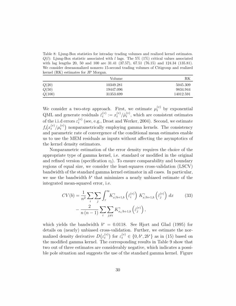
Table 8: Ljung-Box statistics for intraday trading volumes and realized kernel estimates.Q(l): Ljung-Box statistic associated with l lags. The 5% (1%) critical values associatedwith lag lengths 20, 50 and 100 are 31.41 (37.57), 67.51 (76.15) and 124.34 (135.81).We consider deseasonalized nonzero 15-second trading volumes of Citigroup and realizedkernel (RK) estimates for JP Morgan.
We consider a two-step approach. First, we estimate µ(v)t by exponential
QML and generate residuals ε(v)t := x
(v)t /µ
(v)t , which are consistent estimates
of the i.i.d errors ε(v)t (see, e.g., Drost and Werker, 2004). Second, we estimate
fε(x
(v)t /µ
(v)t
)nonparametrically employing gamma kernels. The consistency
and parametric rate of convergence of the conditional mean estimates enableus to use the MEM residuals as inputs without affecting the asymptotics ofthe kernel density estimators.
Nonparametric estimation of the error density requires the choice of theappropriate type of gamma kernel, i.e. standard or modified in the originaland refined version (specification vI). To ensure comparability and boundaryregions of equal size, we consider the least-squares cross-validation (LSCV)bandwidth of the standard gamma kernel estimator in all cases. In particular,we use the bandwidth b∗ that minimizes a nearly unbiased estimate of theintegrated mean-squared error, i.e.
CV (b) =1
n2
∑i
∑j
∫ ∞τ
Kγx/b+1,b
(ε
(v)i
)Kγx/b+1,b
(ε
(v)j
)dx (33)
− 2
n (n− 1)
∑i
∑j 6=i
Kγxi/b+1,b
(ε
(v)j
),
which yields the bandwidth b∗ = 0.0118. See Hjort and Glad (1995) fordetails on (nearly) unbiased cross-validation. Further, we estimate the nor-
malized density derivative D(ε
(v)t
)for ε
(v)t ∈ {0, b∗, 2b∗} as in (15) based on
the modified gamma kernel. The corresponding results in Table 9 show thattwo out of three estimates are considerably negative, which indicates a possi-ble pole situation and suggests the use of the standard gamma kernel. Figure
30
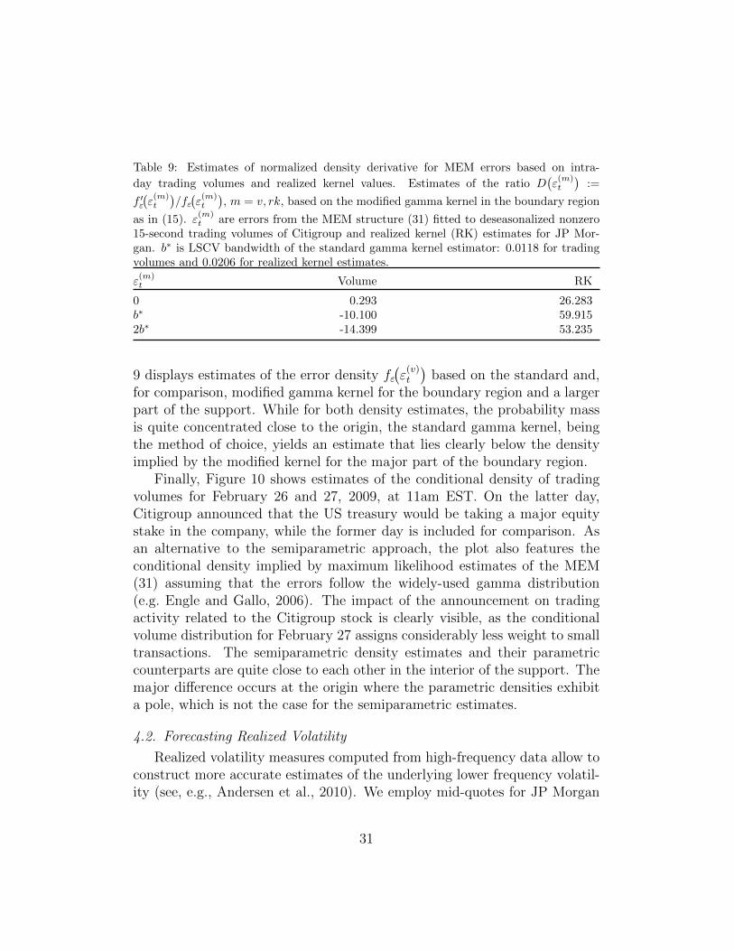
Table 9: Estimates of normalized density derivative for MEM errors based on intra-
day trading volumes and realized kernel values. Estimates of the ratio D(ε(m)t
):=
f ′ε(ε(m)t
)/fε(ε(m)t
), m = v, rk, based on the modified gamma kernel in the boundary region
as in (15). ε(m)t are errors from the MEM structure (31) fitted to deseasonalized nonzero
15-second trading volumes of Citigroup and realized kernel (RK) estimates for JP Mor-gan. b∗ is LSCV bandwidth of the standard gamma kernel estimator: 0.0118 for tradingvolumes and 0.0206 for realized kernel estimates.
ε(m)t Volume RK
0 0.293 26.283b∗ -10.100 59.9152b∗ -14.399 53.235
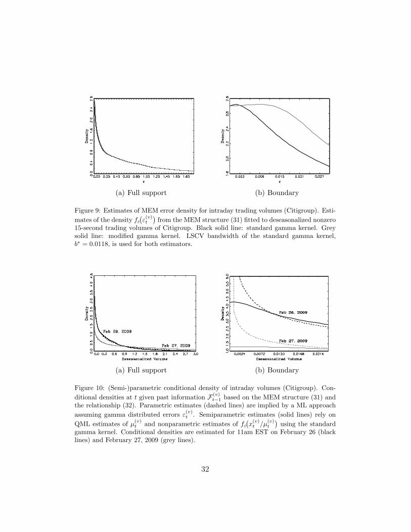
9 displays estimates of the error density fε(ε
(v)t
)based on the standard and,
for comparison, modified gamma kernel for the boundary region and a largerpart of the support. While for both density estimates, the probability massis quite concentrated close to the origin, the standard gamma kernel, beingthe method of choice, yields an estimate that lies clearly below the densityimplied by the modified kernel for the major part of the boundary region.
Finally, Figure 10 shows estimates of the conditional density of tradingvolumes for February 26 and 27, 2009, at 11am EST. On the latter day,Citigroup announced that the US treasury would be taking a major equitystake in the company, while the former day is included for comparison. Asan alternative to the semiparametric approach, the plot also features theconditional density implied by maximum likelihood estimates of the MEM(31) assuming that the errors follow the widely-used gamma distribution(e.g. Engle and Gallo, 2006). The impact of the announcement on tradingactivity related to the Citigroup stock is clearly visible, as the conditionalvolume distribution for February 27 assigns considerably less weight to smalltransactions. The semiparametric density estimates and their parametriccounterparts are quite close to each other in the interior of the support. Themajor difference occurs at the origin where the parametric densities exhibita pole, which is not the case for the semiparametric estimates.
4.2. Forecasting Realized Volatility
Realized volatility measures computed from high-frequency data allow toconstruct more accurate estimates of the underlying lower frequency volatil-ity (see, e.g., Andersen et al., 2010). We employ mid-quotes for JP Morgan
31
(a) Full support (b) Boundary
Figure 9: Estimates of MEM error density for intraday trading volumes (Citigroup). Esti-
mates of the density fε(ε(v)t
)from the MEM structure (31) fitted to deseasonalized nonzero
15-second trading volumes of Citigroup. Black solid line: standard gamma kernel. Greysolid line: modified gamma kernel. LSCV bandwidth of the standard gamma kernel,b∗ = 0.0118, is used for both estimators.
(a) Full support (b) Boundary
Figure 10: (Semi-)parametric conditional density of intraday volumes (Citigroup). Con-
ditional densities at t given past information F (v)t−1 based on the MEM structure (31) and
the relationship (32). Parametric estimates (dashed lines) are implied by a ML approach
QML estimates of µ(v)t and nonparametric estimates of fε
(x(v)t /µ
(v)t
)using the standard
gamma kernel. Conditional densities are estimated for 11am EST on February 26 (blacklines) and February 27, 2009 (grey lines).
32
from January 2006 to December 2009, which corresponds to 983 trading days,and clean the raw data as suggested in Barndorff-Nielsen et al. (2008b). Therealized volatility for day t is simply defined as the sum of squared (mid-quote) returns ri,t, i = 1, . . . , Nt. Barndorff-Nielsen and Shephard (2002)show that, in the absence of noise and with the number of intraday re-turns approaching infinity, this basic estimator is consistent for the latentintegrated volatility, which under regularity conditions provides an unbiasedmeasure of the conditional variance of (daily) returns. In practice, observedprices are contaminated by microstructure effects causing an inconsistency ofthe basic realized volatility estimator (e.g. Hansen and Lunde, 2006). Hence,we consider the noise-robust realized kernel estimator, which was proposedby Barndorff-Nielsen et al. (2008a) and takes the form
x(rk)t := γ0 +
H∑h=1
k
(h− 1
H
)(γh + γ−h) , γh :=
n∑i=1
ri,tri−h,t, (34)
where k(·) is the Parzen kernel and H the bandwidth. The number of re-turns used for the computation of the realized kernel, n, is lower than thetotal number of observations Nt due to the so-called jittering procedure. SeeBarndorff-Nielsen et al. (2008a) for details. Since (filtered) realized kernelestimates are used as inputs for kernel density estimators below, the twobandwidths involved have to be balanced in a way similar to Corradi et al.(2009), who propose nonparametric conditional density estimators for theintegrated volatility. We ensure that their assumption A.1 is met by choos-ing H as in Section 4.3 of Barndorff-Nielsen et al. (2008a). To estimate theso-called noise-to-signal ratio, we follow Barndorff-Nielsen et al. (2008b).
Table 8 shows that the realized kernel estimates exhibit a similar persis-tence as trading volumes, which we account for by following Engle and Gallo(2006) and imposing a flexible MEM structure. Hence, we model the real-
ized kernel value for day t, x(rk)t , analogously to (31), where the assumptions
for the errors ε(rk)t remain the same, while a slightly different specification is
chosen for the conditional mean µ(rk)t (see AppendixA). We compute semi-
parametric estimates of the conditional density fX(x
(rk)t |F
(rk)t−1
)using the same
approach as in Section 4.1, which in the given application, can be consideredas a simple alternative to the fully nonparametric procedure proposed in Cor-radi et al. (2009). As Table 9 reports, the estimates of the normalized densityderivative for the MEM errors are consistently positive, indicating that the
33
(a) Full support (b) Boundary
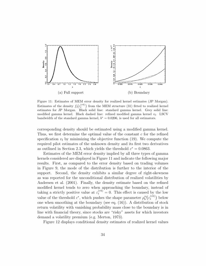
Figure 11: Estimates of MEM error density for realized kernel estimates (JP Morgan).
Estimates of the density fε(ε(rk)t
)from the MEM structure (31) fitted to realized kernel
estimates for JP Morgan. Black solid line: standard gamma kernel. Grey solid line:modified gamma kernel. Black dashed line: refined modified gamma kernel vI. LSCVbandwidth of the standard gamma kernel, b∗ = 0.0206, is used for all estimators.
corresponding density should be estimated using a modified gamma kernel.Thus, we first determine the optimal value of the constant c for the refinedspecification vI by minimizing the objective function (19). We compute therequired pilot estimates of the unknown density and its first two derivativesas outlined in Section 2.3, which yields the threshold c∗ = 0.0863.
Estimates of the MEM error density implied by all three types of gammakernels considered are displayed in Figure 11 and indicate the following majorresults. First, as compared to the error density based on trading volumesin Figure 9, the mode of the distribution is further to the interior of thesupport. Second, the density exhibits a similar degree of right-skewnessas was reported for the unconditional distribution of realized volatilities byAndersen et al. (2001). Finally, the density estimate based on the refinedmodified kernel tends to zero when approaching the boundary, instead oftaking a strictly positive value at ε
(rk)t = 0. This effect is caused by the low
value of the threshold c∗, which pushes the shape parameter ρvIb(ε
(rk)t
)below
one when smoothing at the boundary (see eq. (16)). A distribution of stockreturn volatility with vanishing probability mass close to the boundary is inline with financial theory, since stocks are “risky” assets for which investorsdemand a volatility premium (e.g. Merton, 1973).
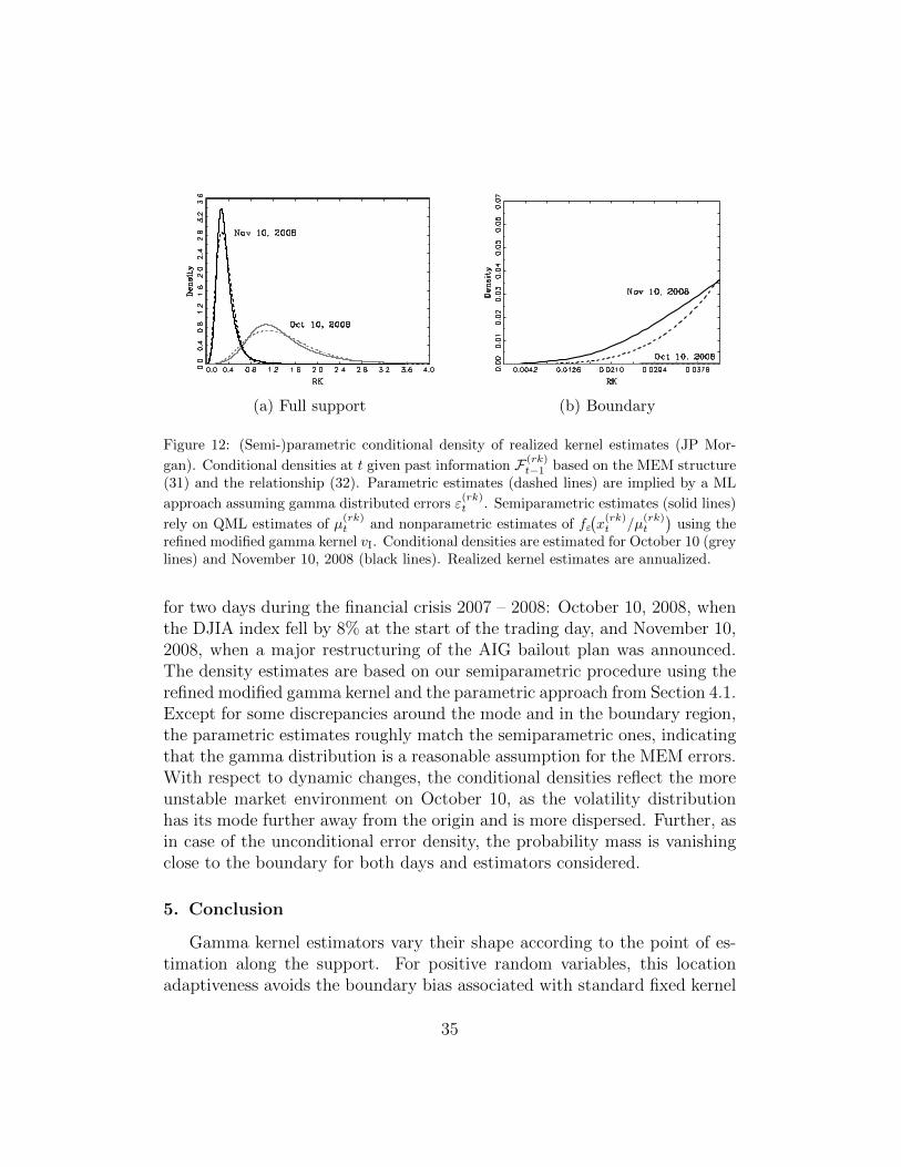
Figure 12 displays conditional density estimates of realized kernel values
34
(a) Full support (b) Boundary
Figure 12: (Semi-)parametric conditional density of realized kernel estimates (JP Mor-
gan). Conditional densities at t given past information F (rk)t−1 based on the MEM structure
(31) and the relationship (32). Parametric estimates (dashed lines) are implied by a ML
rely on QML estimates of µ(rk)t and nonparametric estimates of fε
(x(rk)t /µ
(rk)t
)using the
refined modified gamma kernel vI. Conditional densities are estimated for October 10 (greylines) and November 10, 2008 (black lines). Realized kernel estimates are annualized.
for two days during the financial crisis 2007 – 2008: October 10, 2008, whenthe DJIA index fell by 8% at the start of the trading day, and November 10,2008, when a major restructuring of the AIG bailout plan was announced.The density estimates are based on our semiparametric procedure using therefined modified gamma kernel and the parametric approach from Section 4.1.Except for some discrepancies around the mode and in the boundary region,the parametric estimates roughly match the semiparametric ones, indicatingthat the gamma distribution is a reasonable assumption for the MEM errors.With respect to dynamic changes, the conditional densities reflect the moreunstable market environment on October 10, as the volatility distributionhas its mode further away from the origin and is more dispersed. Further, asin case of the unconditional error density, the probability mass is vanishingclose to the boundary for both days and estimators considered.
5. Conclusion
Gamma kernel estimators vary their shape according to the point of es-timation along the support. For positive random variables, this locationadaptiveness avoids the boundary bias associated with standard fixed kernel
35
estimators, while yielding strictly nonnegative density estimates by construc-tion. We show for various density shapes that, in finite samples, the twooriginal gamma kernel estimators outperform all boundary and boundarycorrected fixed kernel type estimators at the boundary, in particular for set-tings with a large probability mass close to zero. For all other setups and inthe interior of the support, their finite sample performance is comparable tothe one of fixed-type boundary kernels. Moreover, with asymptotic consider-ations and finite sample illustrations we find that, for pole situations at zero,the two gamma kernel estimators differ substantially. In fact, the standardtype is superior to the generally used modified version in this case. There-fore, we suggest a simple criterion to check for such situations. For all othersettings, we propose a refined modified version of the gamma kernel estima-tor, which further improves upon the performance of the modified gammakernel. Our technique is complemented by a data-driven way for choosingthe specification parameters in the new refined gamma kernel. In two appli-cation settings, we demonstrate that, in particular in high-frequency finance,the suggested methodology yields superior results of practical impact.
Possible avenues for improving the performance of the proposed methodseven further are manifold. First, nonparametric multiplicative bias correctiontechniques, as proposed in Hirukawa (2010), could be employed. Second,refined gamma kernel estimators could be combined with a local bandwidthvariation in the spirit of Dai and Sperlich (2010). Finally, modificationssimilar to those suggested for gamma kernels could be developed for theBirnbaum-Saunders-type kernels put forward by Marchant et al. (2013).
Acknowledgements
For constructive comments and suggestions we thank the Co-Editor-in-Chief, Erricos John Kontoghiorghes, an anonymous Associate Editor and twoanonymous referees, as well as the participants of the 2013 European Meet-ing of the Econometric Society and workshops at Humboldt-Universitat zuBerlin. This research is supported by the Deutsche Forschungsgemeinschaft(DFG) via the Collaborative Research Center 649 ”Economic Risk” and viathe DFG grant SCHI-1127.
36
Andersen, T. G., Bollerslev, T., Diebold, F. X., 2010. Parametric and non-parametric measurements of volatility. In: Ait-Sahalia, Y., Hansen, L.(Eds.), Handbook of Financial Econometrics. North Holland, Amsterdam,pp. 67–137.
Andersen, T. G., Bollerslev, T., Diebold, F. X., Labys, P., 2001. The distribu-tion of realized exchange rate volatility. Journal of the American StatisticalAssociation 96 (453), 42–55.
Barndorff-Nielsen, O., Hansen, P., Lunde, A., Shephard, N., 2008a. Designingrealized kernels to measure the ex-post variation of equity prices in thepresence of noise. Econometrica 76, 1481–1536.
Barndorff-Nielsen, O., Hansen, P., Lunde, A., Shephard, N., 2008b. Realisedkernels in practice: trades and quotes. Econometrics Journal 4, 1–32.
Barndorff-Nielsen, O., Shephard, N., 2002. Econometric analysis of realizedvolatility and its use in estimating stochastic volatility models. Journal ofthe Royal Statistical Society, Ser. B. 64, 253–280.
Bauwens, L., Giot, P., 2000. The logarithmic ACD model: an application tothe bid-ask quote process of three NYSE stocks. Annales D’Economie etde Statistique 60, 117–149.
Bouezmarni, T., Rombouts, J. V., 2010a. Nonparametric density estimationfor multivariate bounded data. Journal of Statistical Planning and Infer-ence 140 (1), 139 – 152.
Bouezmarni, T., Rombouts, J. V., 2010b. Nonparametric density estimationfor positive time series. Computational Statistics & Data Analysis 54 (2),245 – 261.
Bouezmarni, T., Scaillet, O., 2005. Consistency of asymmetric kernel den-sity estimators and smoothed histograms with application to income data.Econometric Theory 21 (02), 390–412.
Brownlees, C. T., Cipollini, F., Gallo, G. M., 2010. Intra-daily volume mod-eling and prediction for algorithmic trading. Journal of Financial Econo-metrics 8 (4), 1–30.
37
Chen, S., 1999. Beta kernel estimators for density functions. ComputationalStatistics & Data Analysis 31 (2), 131–145.
Chen, S., 2000. Probability density function estimation using gamma kernels.Annals of the Institute of Statistical Mathematics 52, 471–480.
Corradi, V., Distaso, W., Swanson, N. R., 2009. Predictive density estima-tors for daily volatility based on the use of realized measures. Journal ofEconometrics 150 (2), 119 – 138.
Corsi, F., 2009. A simple approximate long-memory model of realized volatil-ity. Journal of Financial Econometrics, 174–196.
Dai, J., Sperlich, S., 2010. Simple and effective boundary correction for kerneldensities and regression with an application to the world income and engelcurve estimation. Computational Statistics & Data Analysis 54 (11), 2487– 2497.
Drost, F. C., Werker, B. J. M., 2004. Semiparametric duration models. Jour-nal of Business and Economic Statistics 22, 40–50.
Engle, R. F., 2002. New frontiers for ARCH models. Journal of AppliedEconometrics 17, 425–446.
Engle, R. F., Gallo, G. M., 2006. A multiple indicators model for volatilityusing intra-daily data. Journal of Econometrics 131 (1-2), 3–27.
Fernandes, M., Grammig, J., 2005. Nonparametric specification tests for con-ditional duration models. Journal of Econometrics 127, 35–68.
Ferraty, F., Quintela del Ro, A., Vieu, P., 2012. Specification test for condi-tional distribution with functional variables. Econometric Theory 28 (2),363–386.
Gasser, T., Muller, H., 1979. Kernel estimation of regression functions. In:Gasser, T., Rosenblatt, M. (Eds.), Lecture Notes in Mathematics 757.Springer, Heidelberg, pp. 23–68.
38
Hagmann, M., Scaillet, O., 2007. Local multiplicative bias correction forasymmetric kernel density estimators. Journal of Econometrics 141, 213–249.
Hansen, P. R., Lunde, A., 2006. Realized variance and market microstructurenoise. Journal of Business and Economic Statistics 24 (2), 127–161.
Hautsch, N., 2004. Modelling Irregularly Spaced Financial Data: Theory andPractice of Dynamic Duration Models. Springer, Berlin.
Hautsch, N., Malec, P., Schienle, M., 2013. Capturing the zero: a new classof zero-augmented distributions and multiplicative error processes. Journalof Financial Econometrics forthcoming.
Hirukawa, M., 2010. Nonparametric multiplicative bias correction for kernel-type density estimation on the unit interval. Computational Statistics &Data Analysis 54 (2), 473 – 495.
Hjort, N. L., Glad, I. K., 1995. Nonparametric density estimation with aparametric start. The Annals of Statistics 23, 882–904.
Jones, M., 1993. Simple boundary correction for kernel density estimation.Statistics and Computing 3, 135–146.
Jones, M. C., Foster, P. J., 1996. A simple nonnegative boundary correctionmethod for kernel density estimation. Statistica Sinica 6, 1005–1013.
Karunamuni, R. J., Alberts, T., 2005. On boundary correction in kerneldensity estimation. Statistical Methodology 2, 191–212.
Lancaster, T., 1997. The Econometric Analysis of Transition Data. Cam-bridge University Press, Cambridge.
Marchant, C., Bertin, K., Leiva, V., Saulo, H., 2013. Generalized birnbaum-saunders kernel density estimators and an analysis of financial data. Com-putational Statistics & Data Analysis 63 (0), 1 – 15.
Marron, J. S., Ruppert, D., 1994. Transformations to reduce boundary biasin kernel density estimation. Journal of the Royal Statistical Society. SeriesB 56 (4), 653–671.
39
Merton, R., 1973. An intertemporal capital asset pricing model. Economet-rica 41, 867 – 888.
Michels, P., 1992. Asymmetric kernel functions in non-parametric regressionanalysis and prediction. Journal of the Royal Statistical Society. Series D(The Statistician) 41, 439–454.
Quintela del Ro, A., Ferraty, F., Vieu, P., 2011. Analysis of time of occurrenceof earthquakes: a functional data approach. Mathematical Geosciences43 (6), 695–719.
Robinson, P., Henry, M., 2003. Higher-order kernel semiparametric m-estimation of long memory. Journal of Econometrics 114 (1), 1–27.
Scaillet, O., 2004. Density estimation using inverse and reciprocal inversegaussian kernels. Journal of Nonparametric Statistics 16, 217–226.
Schuster, E., 1958. Incorporating support constraints into nonparametric es-timators of densities. Communications in Statistics, Part A - Theory andMethods 14, 1123–1136.
Zhang, S., 2010. A note on the performance of gamma kernel estimators atthe boundary. Statistics and Probability Letters 80, 548–557.
AppendixA. MEM Specifications
For trading volumes, we specify the conditional mean µ(v)t in (31) using
the logarithmic MEM proposed by Bauwens and Giot (2000). The latter
does not require parameter constraints to ensure the positivity of µ(v)t and
implies
lnµ(v)t = ω +
p∑i=1
αi lnx(v)t−i +
q∑i=1
βi lnµ(v)t−i, (A.1)
where the lag structure is chosen according to the Schwartz information cri-terion (SIC).
In case of volatilities, we consider (A.1) with p = 1, but augmented bythe lags of (logarithmic) weekly and monthly realized kernel estimates, which
40
are defined as the averages
x(rk)t,w =:
1
5
4∑j=0
x(rk)t−j and x
(rk)t,m =:
1
20
19∑j=0
x(rk)t−j . (A.2)
This extension is motivated by the widely-used heterogeneous autoregressive(HAR) model for realized volatilities proposed by Corsi (2009) and yields