IEEE TRANSACTIONS ON SIGNAL PROCESSING, VOL. 42, NO. 10, OCTOBER 1994 2195

Nonparametric Multivariate Density Estimation: A Comparative Study

Jenq-Neng Hwang, Member, IEEE, Shyh-Rong Lay, and Alan Lippman

Abstract- This paper algorithmically and empirically studies two major types of nonparametric multivariate density estimation techniques, where no assumption is made about the data being drawn from any of known parametric families of distribution. The first type is the popular kernel method (and several of its variants) which uses locally tuned radial basis (e.g., Gauss- ian) functions to interpolate the multidimensional density; the second type is based on an exploratory projection pursuit tech- nique which interprets the multidimensional density through the construction of several 1-D densities along highly “interesting” projections of multidimensional data. Performance evaluations using training data from mixture Gaussian and mixture Cauchy densities are presented. The results show that the curse of dimen- sionality and the sensitivity of control parameters have a much more adverse impact on the kernel density estimators than on the projection pursuit density estimators.

I. INTRODUCTION N signal-processing applications, most algorithms work I properly if the probability densities of the multivariate

signals (or noises) are known. Unfortunately, in reality these densities are usually not available, and parametric or non- parametric estimation of the densities becomes critically needed. Unlike the parametric density estimation where assumptions are made about the parametric form of the distribution that generates the data, the nonparametric density estimation makes less rigid assumptions about the distribution of the data 1241.

A probability density function (pdf), f ( y ) , of a p- dimensional data y is a continuous and smooth function which satisfies the following positivity and integrate-to-one constraints

Given a set of p-dimensional observed data { y n , n = 1, . . . , N } , the task of multivariate density estimation is to find an estimated function f̂ which “best” approximates the true probability density function f . On the other hand, a probability mass function (pmf) is a discrete function which also satisfies the positivity and sum-to-one constraints and has been successful in some classification and regression applications [2], [19]. The success of a pmf results from

Manuscript received August 23, 1993; revised April 12, 1994. This work was supported by grants from the National Science Foundation under Grant No. ECS-9014243, from NASA under Contract No. NAGW-1702, and by a postdoctoral fellowship from Office of Naval Research under Grant No. N00014-90-J-1478. The associate editor coordinating the review of this paper and approving it for publication was Dr. R. D. Preuss.

The authors are with the Information Processing Laboratory, Department of Electrical Engineering, University of Washington, Seattle, WA 98195 USA.

IEEE Log Number 9403752.

several well developed clustering algorithms (e.g., [ 161) which cluster multidimensional data {yn, n = 1; . . . , N } into several centroids { m k , IC = 1, . . . , K } and the pmf can thus be obtained by estimating the proportion Ck of data population in each cluster. In this paper, we are only dealing with the continuous pdf which has been successfully applied in applications like classifier design [28], image restoration and compression [20], [21], etc.

Traditionally and statistically, the pdf is constructed by locating a Gaussian kernel at each observed datum, e.g., the fixed-width kemel density estimator (FKDE) and the adaptive kemel density estimator (AKDE). Although the FKDE, which constructs a density by placing fixed width kernels at all of the observed data, is widely used for nonparametric density estimation, this method normally suffers from several practical drawbacks [25]. For example, the inability to deal satisfactorily with tails of distributions without oversmoothing the main part of the density. The other is the curse of dimensionality, i.e., the exponentially increasing sample size required to effectively estimate a multivariate density when the number of dimensions increases.

The AKDE [I], [25] is thus introduced to improve the performance of an FKDE. Similar to an FKDE, the AKDE constructs a density by placing kernels at all of the observed data. Unlike an FKDE that uses kernels of fixed width, an AKDE allows the widths of kernels to vary from one point to another. Although the AKDE slightly improves the estimation capability of an FKDE, it does not reduce the high cost incurred in computation and memory storage commonly required in an FKDE.

To overcome the problem of high cost in computation and memory storage, a (clustered) radial basis function (RBF) based kernel density estimator, named RBF network, can be used [14], [20], 1211. The RBF network uses a reduced number of (radial basis) kernels, with each kemel being representative of a cluster of training data, to approximate the unknown density function. This method is often referred as mixture (Gaussian) modeling [23]. The RBF networks are also widely used in regression and classification applications 1181. Similar to the construction of a pmf, the construction of an RBF network requires the determination of the clus- ter centroids { m k } . Furthermore, the estimates of the data correlation and proportion within or between clusters are translated into the bandwidths (as well as orientations) and heights of the (interpolating) Gaussian kernels to be deployed on the cluster centroids so that a smooth and continous pdf can be constructed. The determination of centroids and associated kernel parameters can be accomplished in two-

1053-587X/94$04.00 0 1994 IEEE

2196 IEEE TRANSACTIONS ON SIGNAL PROCESSING, VOL. 42, NO. 10, OCTOBER 1994

stage batch process or can be done simulataneously in an iterative manner. The two-stage batch process starts with acquiring a satisfactory set of cluster centroids, then deter- mine the kemel bandwidths, orientations, and heights through batch statistical analysis in the sense of maximum likelihood [14], [20], [21]. The iterative kernel deploying approaches for construction of RBF density estimators use the iterative expectation-and-maximization (EM) algorithm [ 171, [23], [27], a maximum likelihood optimization procedure, by treating the cluster label that indicates which kernel a datum belong to as missing data and maximizes the likelihood with respect to the kemel parameters (centroids, bandwidths, orientations, and heights). There are some drawbacks of this approach, namely, slow convergence and the sensitivity of the initial label parameter guesses. In some cases where the likelihood is unbounded in certain parameter space, the procedure will diverge if tlfe initial guess is too close to this space. Like most optimization approaches, the EM algorithm also suffers the local optimum issues. In this paper, we only focus on the discussion of two-stage batch process for RBF network construction.

In two-stage batch construction of an RBF network, sequential and batch clustering algorithms are commonly used in determining the cluster centroids [4], [16], [18]. These clustering algorithms perform poorly in the presence of probabilistic outlying data or data of large variations of dynamic range among dimensions, the latter imposing high sensitivity to the selection of distance measures in the clustering. To overcome these difficulties, statistical data sphering technique combined with a centroid splitting generalized Lloyd clustering technique (also known as the LBG algorithm [16]) is used in the robust RBF density estimator construction. This robust construction method has been successfully applied to classification tasks [ 151.

Although the robust RBF construction technique can over- come some of the difficulties encountered in using conven- tional RBF networks for density estimation, it still can not overcome the drawback of the estimators' performance being too sensitive to the settings of some control parameters, e.g., the number of kemels used, the locations of kemels, the orientation of kemels, the kernel smoothing parameters, the excluding threshold radius for data sphering, the size of training data, etc. We are thus motivated to study the statistical projection pursuit density estimation technique [5], [7]. In contrast to the locally tuned kemel methods, where data are analyzed directly in high dimensional space around the vicinity of the kernel centers, a projection pursuit method globally projects the data onto 1-D or 2-D subspaces, and analyzes the projected data in these low dimensional subspaces to construct the multivariate density. More specifically, the projection pursuit first defines some index of interest of a projected configuration (instead of using the variance adopted by the principal component analysis) and then uses a numerical optimization technique to find the projections of most interest [ 121, [ 171. The projection index adopted for density estimation is the degree of departure of the projection data from normal- ity. This technique has been applied to exploratory multivariate data analysis in some statistical tools [ 131.

i

I 1 2 3 -0.051 4 -3 -2 -1 0

Y

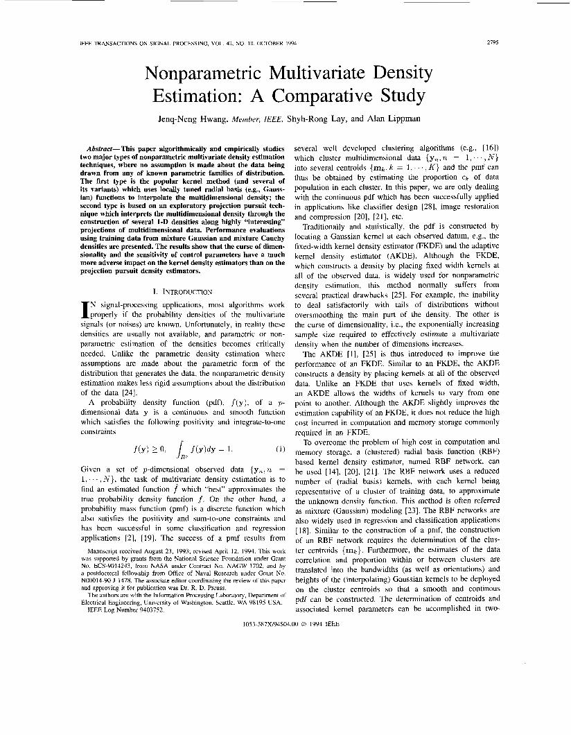
Fig. 1. An example of fixed-width kernel density estimation.

This paper is organized as follows: Section I1 presents various versions of kernel based density estimators: the fixed- width kernel method, the adaptive kemel method, and the robust RBF method. Section 111 discusses the algorithms used for implementing the projection pursuit density estimator. Ex- tensive comparative simulations and discussions of results are performed in Section IV, which is followed by the concluding remarks in Section V.

11. KERNEL-BASED DENSITY ESTIMATION

Given a set of N p-dimensional training data {yn, n = 1,. . . , N } , a multivariate fixed-width kernel density estimator (FKDE), with the kernel function 4 and a fixed (global) kemel width parameter h, gives the estimated density f (y ) for a multivariate data y E RP based on

The kemel function 4 should be chosen to satisfy

4(Y) L 0, and kp 4(Y)dY = 1. (3)

A popular choice of I$ is the Gaussian kernel

which is a symmetric kernel with its value smoothly decaying away from the kemel center. An illustration of FKDE using a small training data set of size 7 is given in Fig. 1.

Normally, the observed data is not equally spread in all directions. It is thus highly desired to pre-scale the data to avoid extreme differences of spread in the various coordi- nate directions. One attractive approach 181 is to first sphere (whiten) the data by a linear transformation yielding data with zero mean and unit covariance matrix, then apply (2) to the sphered data. More specifically, given a set of p-dimensional observed data, {y}, we can define the sphered data z of y to be

(4) = s - w (Y - EY) '

HWANG et al.: NONPARAMETRIC MULTIVARIATE DENSITY ESTIMATION: A COMPARATIVE STUDY 2791

where the expectation E is evaluated through the sample mean, and S E R p X p is the data covariance matrix

S = E [ ( y - E y ) ( y - E Y ) ~ ] = UDUT

or

S-112 = UD-1/2UT. (6)

Note that U is an orthonormal matrix and D is a diagonal matrix. Robust statistics methods [ l l ] can be used for the derivation of the data covariance matrix S.

It can be easily shown that after sphering [Ez] = 0 and E[zzT] = I (the identity matrix). The resulting FKDE for the sphered data performs a more sophisticated density estimation

An optimal kernel width h* for an FKDE can be determined through the minimization of mean integrated squared error (MISE) [25]. For example, the h* for Gaussian kemels was proposed [25] for estimating normally distributed data with unit covariance

h* = AN-&, where A = [4/(2p + l ) ] h . (9)

More complicated methods for determining the kernel width, such as the least-square cross-validation method [25], are also available with increasing complication and computation.

The probabilistic neural network (PNN), introduced by Specht [26], is a multivariate kernel density estimator with fixed kernel width. The kernel width of a PNN is commonly obtained by a trial-and-error procedure. A small value of h causes the estimated density function to have distinct modes corresponding to the locations of the observed data. A larger value of h produces a greater degree of interpolation between data points.

Although the FKDE’s are widely used for nonparametric density estimation, they normally suffer from several practical drawbacks [25]: e.g., the inability to deal satisfactorily with tails of distributions without oversmoothing the main part of the density, and the curse of dimensionality that calls for the requirement of an exponentially increasing sample size to estimate the multivariate density when the number of dimensions increases. The latter drawback also reflects a potential computational burden in using the density estimator after its construction due to the fact that for every observed training datum a kernel is deployed on and an extra term is added in (2).

A. Adaptive Kernel Density Estimator

An improved alternative to an FKDE is the adaptive kernel density estimator (AKDE) [25]. Similar to an FKDE, an AKDE constructs the density by placing a kernel on every observed datum, but it allows the kernel width to vary from one point to another. The intent is to use different widths of kernels

0.4

0.35 -

0 1 0 051 4 -3 -2 -1

2 Y

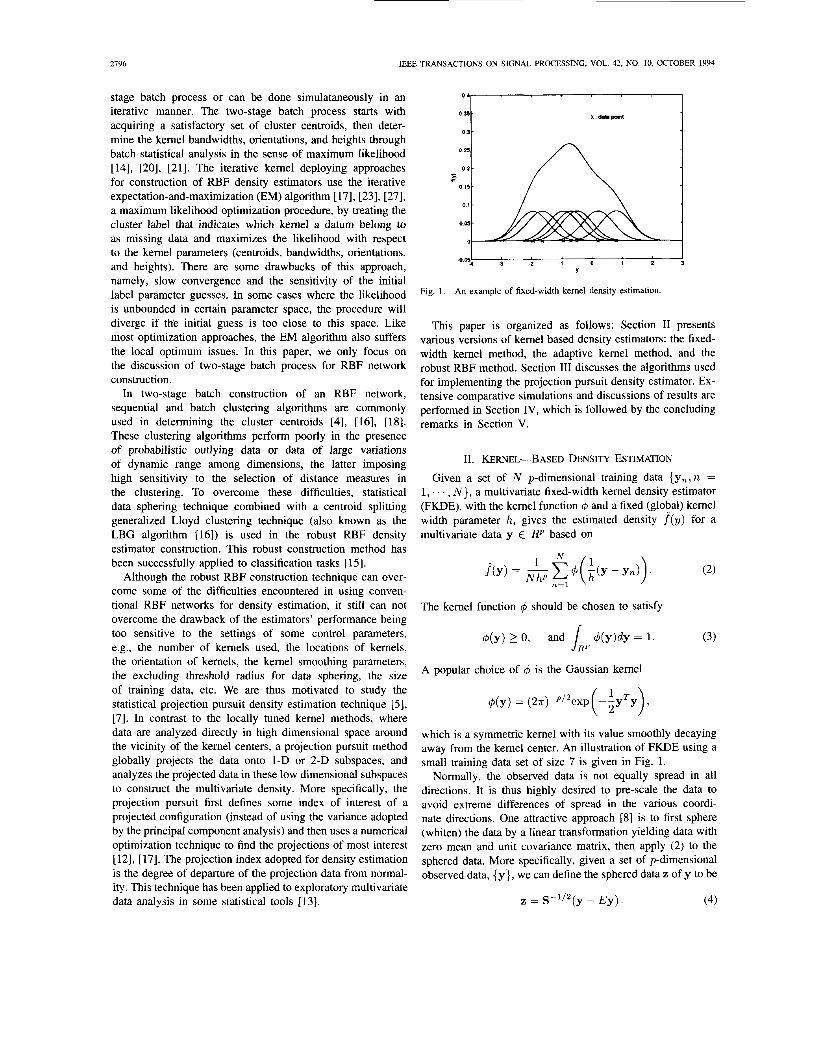
Fig. 2. An example of adaptive kernel density estimation.

in regions of different smoothness. This method adopts a two- step algorithm for computing a data-adaptive kernel width. The algorithm can be summarized as follows:

Step 0: Sphere the observed data { y , } to be { z n } , so that E[z ] = 0 and E[zzT] = I.

Step I : Find a pilot estimate f ( z ) that satisfies f ( z n ) > 0, Vn.

Step 2: Set the local width factor A, _to be ( f ( z n ) / g ) - ’ , where g is the geometric mean of f ( z ) , i.e., logg =

log f ( z i ) , and y is a user defined sensitivity parameter satisfying 0 5 y 5 1.

Step 3: Construct the adaptive kernel estimate f ( z ) by

where h is still the global width parameter used in (2). A natural pilot estimate would be a kernel estimate with fixed optimal kernel width (see (9)). The larger the y, the more sensitive the performance will be to the selection of pilot density. It is quite common to set y = [l], [25]. The estimate f of an AKDE using the small data set of size 7 is illustrated in Fig. 2.

B. Radial Basis Function Density Estimator

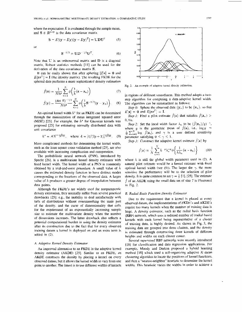
Due to the requirement that a kernel is placed at every observed datum, the implementations of FKDE’s and AKDE’s require too many kernels when the number of training data is huge. A density estimator, such as the radial basis function (RBF) network, which uses a reduced number of (radial basis) kernels with each kernel being representative of a cluster of training data, is highly desired. As shown in Fig. 3, the training data are grouped into three clusters, and the density is estimated through constructing three kernels of different heights and widths on each cluster center.

Several supervised RBF networks were recently introduced [ 181 for classification and data regression applications. For example, Moody and Darken proposed a hybrid learning method [18] which used a self-organizing adaptive K-mean clustering algorithm to locate the positions of kernel functions, and then a “nearest-neighbor’’ heuristic to determine the kernel widths. This heuristic varies the widths in order to achieve a

2798 IEEE TRANSACTIONS ON SIGNAL PROCESSING, VOL. 42, NO. 10, OCTOBER 1994

0.4

0.3s - 1

. o . w m 4 - 3 . 2 - 1 0 1 2 3

Y

Fig. 3. An example of radial basis function-based density estimation.

certain amount of response overlap between each unit and its neighbors. Finally, a least mean squares (LMS) supervised training rule is used for the updating of the heights of the deployed kernels.

1) Data Sphering and Outlier Removing: Since a density estimation task is an unsupervised learning task, a few modifications of the learning procedures for RBF classifi- catiodregression networks are needed. Since an RBF network possesses a local tuning property, the positions of the kernels searched by the clustering algorithm should cover the areas which are most representative of the data in the region around the cluster centers. Unfortunately, most clustering methods are vulnerable to the data outliers which are generated by long-tailed portion of the density. In the classification applications, some outlying training data are useful and can be carefully regularized to increase the generalization capability of the classifiers [22]. However, the outlying training data in a density estimation application usually carry very little information about the density and do not represent any meaningful isolated class as in a classification application. If the RBF network construction is based on the FKDE or AKDE, where a symmetric kernel is placed on every observed training data, the outlying data will not play a significant role in approximating the true density since the amount of outlying data are usually quite small. On the other hand, when clustering techniques are adopted to reduce the number of kernels deployed in an RBF construction, the outlying data play a more significant role. More specifically, most clustering algorithms are types of least squares estimators which are sensitive to outliers. Therefore, we are motivated to remove the outliers after the data sphering and before the data clustering processes [7], 1151. An additional benefit of applying data sphering before data clustering is to simplify the correlation structures of the data so that the distance measures used in the clustering algorithm can also be simplified since different dimensions of the non-sphered data have different scales.

Our RBF density estimation starts with data sphering on the observed training data to get rid of probabilistic outliers and at the same time, if desired, to normalize the spread of data in all directions to facilitate the data clustering. All sphered data with larger norm (e.g., llzll 2 ,O, where p is a prespecified threshold) are excluded for clustering. This data sphering and

outlier removing process continues for several iterations until no outlying data can be removed.

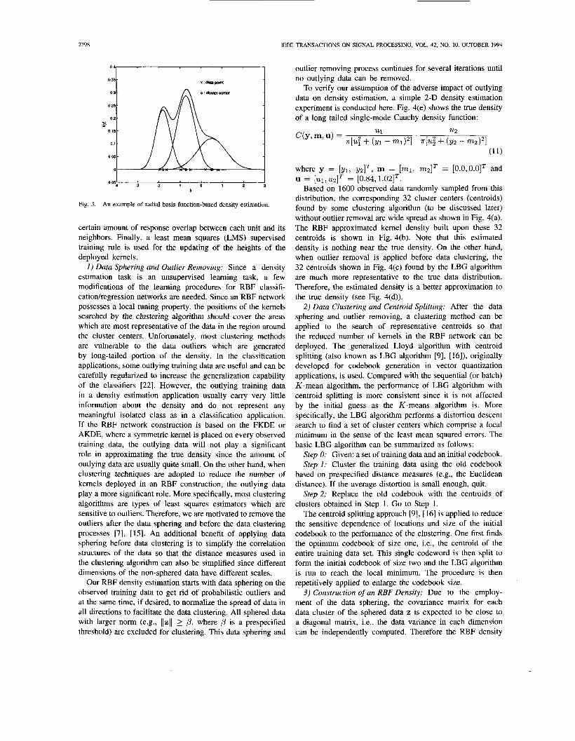
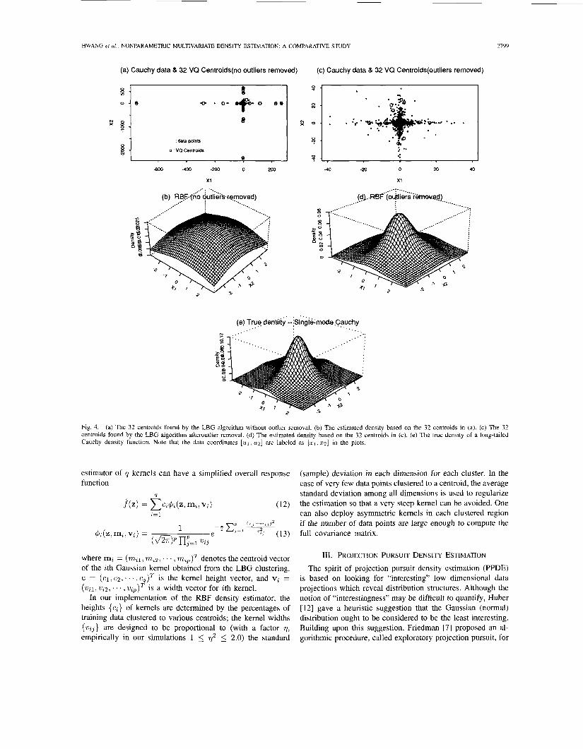
To verify our assumption of the adverse impact of outlying data on density estimation, a simple 2-D density estimation experiment is conducted here. Fig. 4(e) shows the true density of a long tailed single-mode Cauchy density function:

where y = [ y l , 9zlT, m = [ml, mzIT = [O.O,O.OIT and

Based on 1600 observed data randomly sampled from this distribution, the corresponding 32 cluster centers (centroids) found by some clustering algorithm (to be discussed later) without outlier removal are wide spread as shown in Fig. 4(a). The RBF approximated kernel density built upon these 32 centroids is shown in Fig. 4(b). Note that this estimated density is nothing near the true density. On the other hand, when outlier removal is applied before data clustering, the 32 centroids shown in Fig. 4(c) found by the LBG algorithm are much more representative to the true data distribution. Therefore, the estimated density is a better approximation to the true density (see Fig. 4(d)).

2) Data Clustering and Centroid Splitting: After the data sphering and outlier removing, a clustering method can be applied to the search of representative centroids so that the reduced number of kernels in the RBF network can be deployed. The generalized Lloyd algorithm with centroid splitting (also known as LBG algorithm [9], [16]), originally developed for codebook generation in vector quantization applications, is used. Compared with the sequential (or batch) K-mean algorithm, the performance of LBG algorithm with centroid splitting is more consistent since it is not affected by the initial guess as the K-means algorithm is. More specifically, the LBG algorithm performs a distortion descent search to find a set of cluster centers which comprise a local minimum in the sense of the least mean squared errors. The basic LBG algorithm can be summarized as follows:

Step 0: Given: a set of training data and an initial codebook. Step 1: Cluster the training data using the old codebook

based on prespecified distance measures (e.g., the Euclidean distance). If the average distortion is small enough, quit.

Step 2: Replace the old codebook with the centroids of clusters obtained in Step 1. Go to Step 1.

The centroid splitting approach [9], [16] is applied to reduce the sensitive dependence of locations and size of the initial codebook to the performance of the clustering. One first finds the optimum codebook of size one, i.e., the centroid of the entire training data set. This single codeword is then split to form the initial codebook of size two and the LBG algorithm is run to reach the local minimum. The procedure is then repetitively applied to enlarge the codebook size.

3) Construction of an RBF Density: Due to the employ- ment of the data sphering, the covariance matrix for each data cluster of the sphered data z is expected to be close to a diagonal matrix, i.e., the data variance in each dimension can be independently computed. Therefore the RBF density

U = [ u ~ , u z ] ~ = [0.84, 1.O2IT.

HWANG et al.: NONPARAMETRIC MULTIVARIATE DENSITY ESTIMATION: A COMPARATIVE STUDY 2799

(a) Cauchy data 8 32 VQ Centroids(n0 outliers removed) (c) Cauchy data & 32 VQ Centroids(out1iers removed)

data points

o vacentrolds e A

8

.... I -*..-

(b) RBFfno outliei’sr~moved) .,.-

-40 -20 0 20 40

XI _..-._ ..- * .._

--..__ (dj..ReF* (o@ ers’i-emwed) _..- ._..

. , .. (e) True den.sity -- iSingiermoda.Cauchy

Fig. 4. (a) The 32 centroids found by the LBG algorithm without outlier removal. (b) The estimated density based on the 32 centroids in (a). (c) The 32 centroids found by the LBG algorithm afteroutlier removal. (d) The estimated density based on the 32 centroids in (c). ( e ) The true density of a long-tailed Cauchy density function. Note that the data coordinates [ U I , U Z ] are labeled as [ s ~ , . c * ] in the plots.

estimator of q kernels can have a simplified overall response function

(sample) deviation in each dimension for each cluster. In the case of very few data points clustered to a centroid, the average

the estimation so that a very steep kernel can be avoided. One can also deploy asymmetric kernels in each clustered region

4 standard deviation among all dimensions is used to regularize . f (z) = CC;~;(Z, mi, vi) (12)

k l

(2, -m,, I* if the number of data points are large enough to compute the e-’ ‘‘?j (13) full covariance matrix. 1

h ( Z , ”, VL) = ( d m p n;=, VZJ

where mi = ( m i l , m;2, . . . , mip)T denotes the centroid vector of the ith Gaussian kernel obtained from the LBG clustering. c = (c1 , c2, . . . , cq)* is the kernel height vector, and vi = ( i i ; ~ , w;2, . . . , v ; ~ ) ~ is a width vector for ith kemel.

In our implementation of the RBF density estimator, the heights { c ; } of kernels are determined by the percentages of training data clustered to various centroids; the kernel widths { w i j } are designed to be proportional to (with a factor 71, empirically in our simulations 1 5 v2 5 2.0) the standard

111. PROJECTION PURSUIT DENSITY ESTIMATION The spirit of projection pursuit density estimation (PPDE)

is based on looking for “interesting” low dimensional data projections which reveal distribution structures. Although the notion of “interestingness” may be difficult to quantify, Huber [12] gave a heuristic suggestion that the Gaussian (normal) distribution ought to be considered to be the least interesting. Building upon this suggestion, Friedman [7] proposed an al- gorithmic procedure, called exploratory projection pursuit, for

2800 IEEE TRANSACTIONS ON SIGNAL PROCESSING, VOL. 42, NO. 10, OCTOBER 1994

nonparametric multivariate density estimation. In this PPDE procedure, five steps are involved:

Data Sphering: Simplify the location, scale, and correla- tion structures and remove outliers (as discussed in RBF density estimators, see Section 1I.B). Projection Index: Indicate the degree of interestingness of different projection directions. Optimization Strategy: Search efficiently the direction of maximal projection index. Structure Removing: Perform 1-D density estimation on the projection data and transform the data to remove this structure. Density Formation: Combine the 1-D densities from all searched interesting directions to form the multivariate density function.

A. Projection Index: Which Projection Direction is Interesting ?

It is known that all projections of a multivariate Gaussian density are Gaussian, and therefore evidence for the data being non-Gaussian in any projection is evidence against the data being multivariate joint Gaussian. One intuitive definition of projection index f ( a ) , which indicates how close the probability fa(.) of the 1-D projection data, z = a T z along a direction n, being Gaussian (where z is the sphered version of y), is [lo]

1 - z 2 00

j ( a ) = ( f a ( x ) - g(x))’dz, with g(z) = ---e?. 6 (14)

A projection direction a that maximizes f ( a ) yields a pro- jected distribution that exhibit clustering (multimodality) or other kinds of nonlinear structure. If we transform the data 2

by the following equation

L

T = 2G(z) - 1 = 2G(aTz) - 1, T E [-1,1] (15)

where G(z) is the standard normal cumulative distribution function (CDF)

/x e G d t . (16)

According to the fundamental theorem of random variable transform

1 G(x) = ~ 6 -cc

therefore we can rewrite (14) in terms of T as

44 = l1 29(2)(f?.(T) - 1/2)’dr

= L12g(G-’(?))(f?.(r) - 1/2)’dr. (18)

Friedman [7] adopted a slightly different form for the projection index I ( a )

I ( a ) = [p) - 1/2)2dT

= J: f,2(T)dT - l /2 . (19)

Note that if x is Gaussian distributed, then f , . ( ~ ) = 3, Vr and projection index I ( a ) is zero. The more departure of the distribution of 2 from normality, the larger the value of index I ( a ) . Since T E [-1,1], fr(r) can be expanded in terms of orthogonal Legendre polynomials { $ j ( ~ ) , j = 0, . . . , J } , i.e., fr(T) = C , J = O W j ( T )

The orthogonal Legendre polynomials have recursive relation as follows

Through the orthogonal property, the weighting coefficients { b j } can be computed via sample average

where J”, $ j ( r ) f ? . ( ~ ) d r = E?.[$j(r)] is approximated by sample average. Therefore, (19) can be rewritten as

B. Optimization Strategy: The Search for a Best Projection

Once the analytical form of the projection index is defined, its gradient with respect to a projection direction a can be derived as (under the constraint aTa = 1 [7]

where the derivative of each Legendre polynomial can be easily calculated by the recursive formula

HWANG et al.: NONPARAMETRIC MULTIVANATE DENSITY ESTIMATION: A COMPARATIVE STUDY

8-

6-

4 -

A hybrid optimization strategy [7] was used to search for the most interesting projection direction. A "coarse stepping optimizer" is first applied to perform a search on main axes (principal component directions) and their combination direc- tions so that an initial estimate for a maximum can be quickly reached. A "gradient directed optimizer" (steepest ascent) is then adopted to fine-tune the projection direction to ascend to a (local) maximum of projection index.

2 -

0 -

-2

C. Structure Removal: Gaussianize Data Along the Projection

To construct a PPDE, several interesting projections are usually required. After an interesting projection Q: is found, we have to remove the least Gaussian structure along Q: to avoid future search of this direction again, in other words, we have to "Gaussianize" the data along a without affecting the density along other directions. Let's denote the I-D projection data before and after Gaussianization as x and 2, respectively. Gaussianization of the 1-D projection data z is accomplished by

. . . *. . . . * . . . . . . . . . .r .... :*. .... . --. , ..... ......... . . . +.+.;...,.: * ... . . ..* . , . . . . . . : . ..-. .'at... " . ... L .*.*::.l.'i . .

- . -. - . . . - ......

,e .. < - . ** . ; -.?... :... s

i s . . . . . . . . . . . . ..,; . ;, . . . . .. - . . .

where G-l is the inverse of the standard normal CDF given in (16) and F,(x) is an estimate of the CDF of 2. Friedman [7] suggested to use the empirical CDF (x) = rank( z ) / N - &, where rank(x) is the rank of x among all the N observed data points. However, this empirical distribution formulation is quite inaccurate and usually results in very unsmooth estimated densities. We estimate F, (x) through intergration of a linear interpolation of f,(x). Based on this modification, we then have to compute the high dimensional structure removed data Z from z. Let U be an orthonormal matrix, U = [ ~ , @ 1 , @ 2 , . . . , p ~ - 1 ] ~ , where {p i } are found through Gram-Schmidt algorithm

The same projection index maximization procedure is reap- plied to the data z for the searching of other interesting projection structures until the multivariate data is close to Gaussian distribution in any direction. It was noted [7] that "Gaussianizing" along one solution projection perturbs the normality along previously found solution projections so that they no longer have exactly zero interest. However, empirical experience indicates that the induced perturbation is very small. If desired, the backfitting procedure [SI can be reapplied to the previous projections.

D. Density Formation: From Projections to Density

The density of the original sphered data is estimated by com- bining those projected 1 -D density estimations. The density relation between the high-dimensional data z ( ~ ) and z ( ~ - ~ ) is (where z ( ~ ) is the structure removed data of z(,-l) along

.. .......

e , ... .: 5 : .. .... j.: ... .. : . . . . . . - ,--. r .. * *

,. -::-#.:. . . . . ... .-:*:.:. . . . . . . . - <

~

2801

-2 -4 0 2 4 6 8 -41

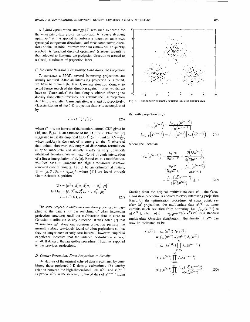
Fig. 5. Four hundred randomly sampled Gaussian mixture data.

the mth projection a,)

where the Jacobian

Starting from the original multivariate data z(O), the Gaus- sianization procedure is applied to every interesting projection found by the optimization procedure. At some point, say after N I projections, the multivariate data z(*') no more exhibits much deviation from normality, i.e., f , , (.("I) z g(z("")), where y(z) = h e x p ( - z T z / 2 ) is a standard multivariate Gaussian distribution. The density of z(O) can now be estimated to be

2802 IEEE TRANSACTTONS ON SIGNAL PROCESSING, VOL. 42, NO. 10, OCTOBER 1994

Fig. 6. (a) The true density of a Gaussian mixture. (b) The PPD eestimate, fml(z(l))Jl(z(o)), after the first projection. (c) The PPDE estimate, fa2(~(2))J2(z(')) Ji(z(')), after the second projection. (d) The PPDE estimate, j n , ( z ( 3 ) ) J 3 ( z ( 2 ) ) . J z ( z ( ' ) ) J l ( z ( O ) ) , after the third projection. Note that the data coordinates [:I, 221 are labeled as [SI ~ x.21 in the plots.

The 1-D probability fam ( Q ; Z ( ~ - ~ ) ) is estimated according to (17), i.e., fa = 2g(z)f,(r), or more specifically

Due to the polynomial form of the projection index and the recursive relations in the polynomials and its first derivatives, PPDE can be rapidly computed. Figs. 5 and 6 gives a step-by- step illustration of the PPDE construction from the first three projections using 400 training data sampled from a Gaussian mixture.

IV. COMPARATIVE SIMULATIONS We have discussed the nonparametric "kernel-based" and

"projection-pursuit'' density estimators from structural and computational viewpoints. We carry out in this section a detailed comparison of performance among these methods via a simulation study.

A. Simulated Data

Three types of multidimensional (2-D-5-D) data of Gauss- ian and Cauchy mixture distributions are generated. The Cauchy distribution has a long tail while the Gaussian distri- bution does not. The data are generated such that all elements in the same data vector are independent of each other. These

data have the following distribution forms

K

Gaussian Mixture: c k ~ ( y , mk, V k )

k - 1 K

Cauchy Mixture: C k c ( y , mk, u k ) (32) k = l

with the constraint ckl C k = 1 and

(33)

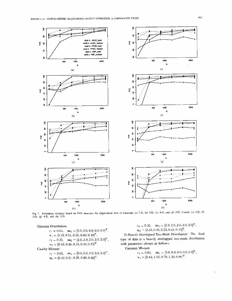
1) Single Mode Distribution: The first type of data is a single-mode distribution with parameters chosen as follows (note that, for 2 -D4-D cases we take the first 2-D-4-D elements from the 5-D parameter set as shown below):

Gaussian Distribution: c = 1.0, v = [0.84,1.02,0.70,1.20, 0.96IT.

c = 1.0, U = [0.84,1.02,0.70, 1.20,0.961T.

m = [o.o,o.o, O.O,O.O, o . o ] ~ ,

Cauchy Distribution: m = [o.o, 0.0, 0.0, 0.0, o . o ] ~ ,

2 ) Lightly Overlapped Two-Mode Distribution: The sec- ond type of data is a lightly overlapped two-mode distribution with parameters chosen as follows:

2803 HWANG et al.: NONPARAMETRIC MULTIVARIATE DENSITY ESTIMATION: A COMPARATIVE STUDY

dash A ' AKDE-test so l i A : AKDE-median

dash o : PPDE-best so l i o : PPDE-median

dash x : RBF-best so l i x . REF-mediin

500 lo00 Moo

N

(a)

8 SI

3

e k

500 loo0

N

(b)

m

W

P

MO lo00

N

(C)

Moo

0

500 lo00 5ooo

N

(d)

500 lo00

N

(0

Fig. 7. Estimation accuracy based on PVE measures for single-mode data of Gaussian (a) 2-D, (b) 3-D, (c) 4-D, and (d) 5-D; Cauchy (e) 2-D, (f) 3-D, (g) 4-D, and (h) 5-D.

Gaussian Distribution: c1 = 0.65, v1 = [0.42,0.51, 0.35,0.60,0.481T. c2 = 0.35, v2 = [0.33,0.46,0.53,0.43,0.451T.

ml = [O.O,O.O,O.O,O.O,O.O]T,

m2 = [2.0,2.0,2.0,2.0, 2.OlT,

Cauchy Mixture: c1 = 0.65, ' ml = [O.O,O.O,O.O,O.O,O.O]T, ~1 = [0.42,0.51, 0.35,0.60,0.48lT.

c2 = 0.35, m2 = [2.0,2.0,2.0,2.0,2.0IT,

3) Heavily Overlapped Two-Mode Distribution: The third type of data is a heavily overlapped two-mode distribution with parameters chosen as follows:

c1 = 0.65, VI = [0.84,1.02,0.70, 1.20,0.961T.

~2 = [0.33,0.46,0.53,0.43, 0.451T.

Gaussian Mixture: ml = [O.O,O.O,O.O,O.O,O.O]T,

2804 IEEE TRANSACTIONS ON SIGNAL PROCESSING, VOL. 42, NO. 10, OCTOBER 1994

(e) True den’sity‘-- /Skgie+nsde .Cauchy

_ . ’

Fig. 8. 2-D Cauchy (e) True density. (0 PPDE estimation. (g) AKDE estimation. (h) RBF estimation.

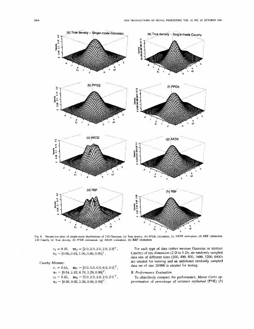
Perspective plots of single-mode distributions of 2-D Gaussian: (a) True density. (b) PPDE estimation. (c) AKDE estimation. (d) RBF estimation;

c2 = 0.35, ~2 = [0.66,0.92,1.06,0.86, 0.901T.

m2 = [2.0,2.0,2.0,2.0, 2.OIT, For each type of data (either mixture Gaussian or mixture Cauchy) of any dimension (2-D to 5-D), six randomly sampled data sets of different sizes (200, 400, 800, 1600, 3200, 6400) are created for training and an additional randomly sampled data set of size 20000 is created for testing.

Cauchy Mixture: c1 = 0.65, ml = [O.O,O.O,O.O,O.O,O.O]T, ~1 = [0.84,1.02,0.70, 1.20,0.961T. cz = 0.35, uz = [0.66,0.92,1.06,0.86, 0.901T.

B. Per$ormance Evaluation To objectively compare the performance, Monte Carlo ap-

proximation of percentage of variance explained (PVE) [ 5 ] m2 = [2.0,2.0,2.0,2.0, 2.OIT,

2805 HWANG et al.: NONPARAMETRIC MULTIVARIATE DENSITY ESTIMATION: A COMPARATIVE STUDY

E -

8

8

: g

. . . . . . . . . e ........ e o' ....... o/

. . . . . . . .

solid o : PPDE-medin dashx:RBF-bos( I I soli x : RBF-median I

500 lo00

N

(C)

Moo

04 500 lo00

N

(e)

........ ....... ........ . . . . . . .

- e d - 1 - q . .

W

8 J 1

500 lo00

N

(g)

Moo

5 1

500 loo0

N

(h)

5Ooo

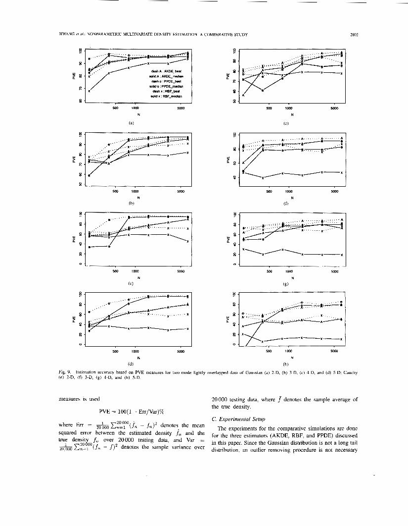
Fig. 9. (e) 2-D, (f) 3-D, (g) 4-D, and (h) 5-D.

Estimation accuracy based on PVE measures for two-mode lightly overlapped data of Gaussian (a) 2-D, (b) 3-D, (c) 4-D, and (d) 5-D; Cauchy

measures is used 20000 testing data, where f denotes the sample average of the true density.

C. Experimental Setup PVE = 100( 1 - Em/Var)%

20 000 where Err = 5TkiG cn=l (.fn - f n ) 2 denotes the mean

Over 20000 testing data, and Var = true den,s$joo f n

The experiments for the comparative simulations are done

in this paper. Since the Gaussian distribution is not a long tail

'quared between the estimated density .fn and the for the three estimators ( A m E , RBF, and PPDE) discussed

cn=1 ( f n - f l 2 denotes the variance Over distribution, an outlier removing procedure is not necessary

2806 IEEE TRANSACTIONS ON SIGNAL PROCESSING, VOL. 42, NO. 10, OCTOBER 1994

(a) True.d.ensity'-: lightly 0verlappedGairssian.Mixture 2 . . . . . -

3

......... (b):PPDE ........... "._ .*

. .

..... : I

(e) True .densi$' -- lightly: overlapped'Cau&hhy Mxture '"0 -:... ,. ,

... ....... (c);AKDE . . . . . . . . . . __ ';.

: . ......... . . . . . . . ....

. . . .

" . _ (g);AKDE

. . . . . . . (hj RBF' ' ' . . .....

Fig. 10. RBF estimation; 2-D Cauchy (e) True density. (f) PPDE estimation. (8) AKDE estimation. (h) RBF estimation.

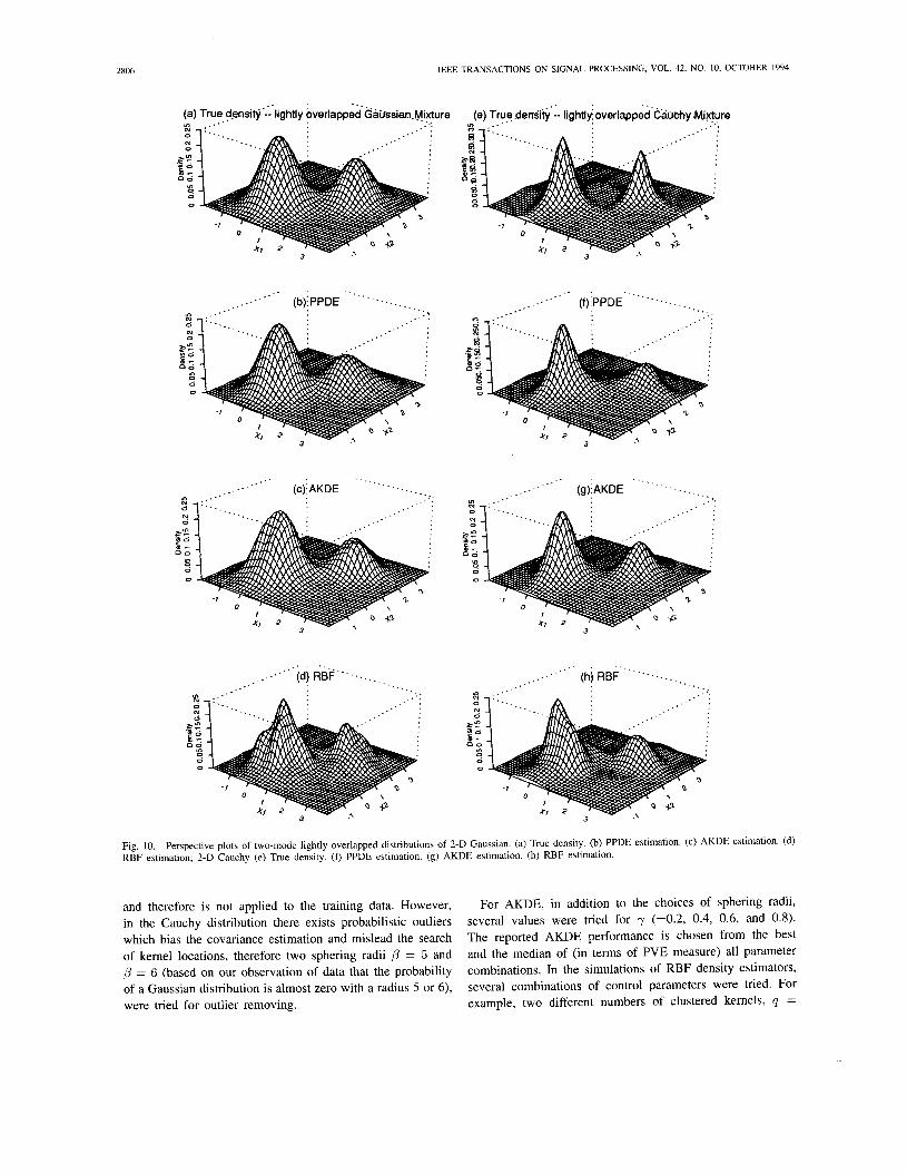
Perspective plots of two-mode lightly overlapped distributions of 2-D Gaussian. (a) True density. (b) PPDE estimation. (c) AKDE estimation. (d)

and therefore is not applied to the training data. However, in the Cauchy distribution there exists probabilistic outliers which bias the covariance estimation and mislead the search of kernel locations, therefore two sphering radii /3 = 5 and /3 = 6 (based on our observation of data that the probability of a Gaussian distribution is almost zero with a radius 5 or 6), were tried for outlier removing.

For AKDE, in addition to the choices of sphering radii, several values were tried for y (=0.2, 0.4, 0.6, and 0.8). The reported AKDE performance is chosen from the best and the median of (in terms of PVE measure) all parameter combinations. In the simulations of RBF density estimators, several combinations of control parameters were tried. For example, two different numbers of clustered kernels, q =

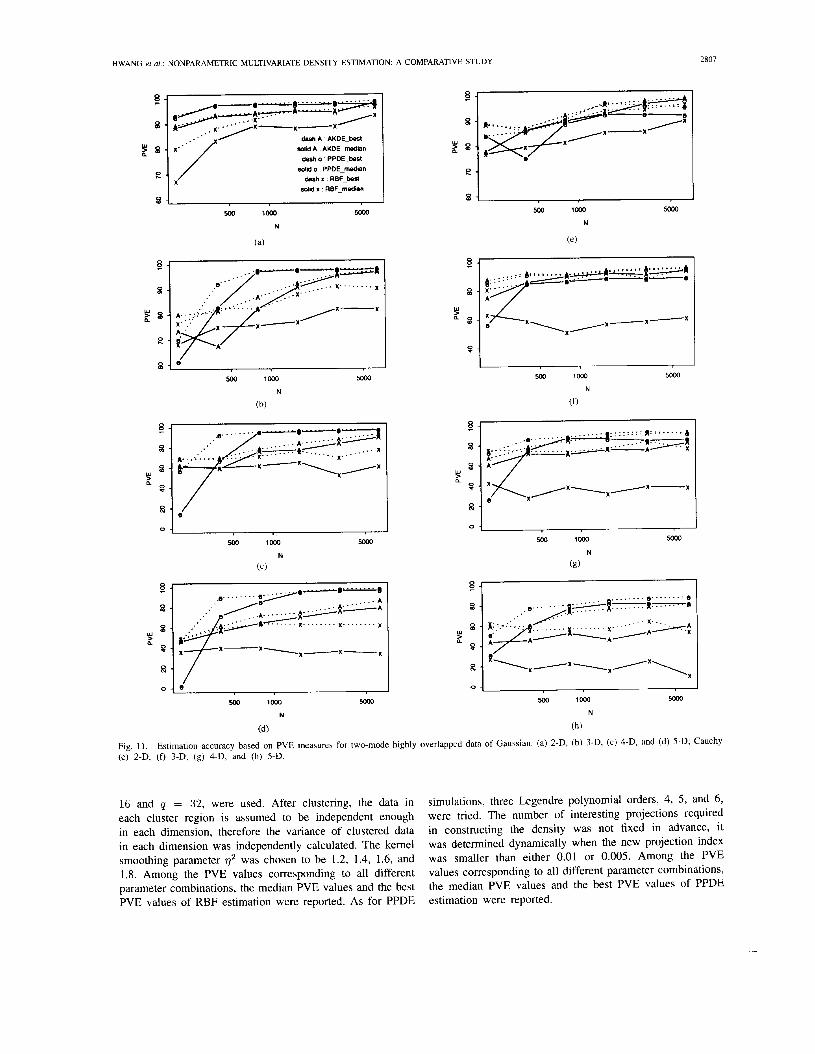
HWANG er al.: NONPARAMETRIC MULTIVARIATE DENSITY ESTIMATION: A COMPARATIVE STUDY 2807

500 lo00

N

(a)

Moo

. -e- ........

. A '

A. X ' &/ ........... . X-x ' . /X-X

A. . B e'

500 lo00 Moo

N

(b)

...... e-@-.- ....... .... x .... ....

1 e' 0

500 lo00 Moo

N (C)

500 lo00

N

(d)

Moo

500 lo00 Moo

N

(e)

500 loo0 Moo

N

(f)

Moo

0

500 lo00 Moo

N

(h)

Fig. 11. (e) 2-D, (f) 3-D, (g) 4-D, and (h) 5-D.

Estimation accuracy based on PVE measures for two-mode highly overlapped data of Gaussian. (a) 2-D, (b) 3-D, (c) 4-D, and (d) 5-D; Cauchy

16 and q = 32, were used. After clustering, the data in each cluster region is assumed to be independent enough in each dimension, therefore the variance of clustered data in each dimension was independently calculated. The kernel smoothing parameter q2 was chosen to be 1.2, 1.4, 1.6, and 1.8. Among the PVE values corresponding to all different parameter combinations, the median PVE values and the best PVE values of RBF estimation were reported. As for PPDE

simulations, three Legendre polynomial orders, 4, 5 , and 6, were tried. The number of interesting projections required in constructing the density was not fixed in advance, it was determined dynamically when the new projection index was smaller than either 0.01 or 0.005. Among the PVE values corresponding to all different parameter combinations, the median PVE values and the best PVE values of PPDE estimation were reported.

2808 IEEE TRANSACTIONS ON SIGNAL PROCESSING, VOL. 42, NO. 10, OCTOBER 1994

. .. (a) True densjty.-'-'h'ighly Qverlapped Gauss@ Mixture (e) True denqity .I'highlyove;i~p~d.Cauchy Mixture

.... . .

4

Fig. 12. RBF estimation; 2-D Cauchy (e) True density. (f) PPDE estimation. (g) AKDE estimation. (h) RBF estimation.

Perspective plots of two-mode highly overlapped distributions of 2-D Gaussian. (a) True density. (b) PPDE estimation. (c) AKDE estimation. (d)

D. Simulation Results and best) PVE performance plots for two-mode Gaussian and Cauchy lightly overlapped data of various dimensions versus Various training data Sizes. The perspective plots of the true and estimated densities (based on 1600 data) corresponding to the median PVE for two-mode Gaussian and Cauchy lightly overlapped distribution of 2-D data are shown in Fig. 10. Fig. 11 shows the (median and best) PVE performance plots

~ i ~ . 7 shows the (median and best) PVE perfomance plots for single-mode Gaussian and Cauchy data of various dimensions versus various training data sizes. The perspective plots of the true and estimated densities (based on 1600 data) corresponding to the median PVE for single-mode distribution of 2-D data are shown in Fig. 8. Fig. 9 shows the (median

HWANG et al.: NONPARAMETRIC MULTIVARIATE DENSITY ESTIMATION: A COMPARATIVE STUDY 2809

for two-mode Gaussian and Cauchy heavily overlapped data of various dimensions versus various training data sizes. The perspective plots of the true and estimated densities (based on 1600 data) corresponding to the median PVE for two-mode Gaussian and Cauchy heavily overlapped data of 2-D data are shown in Fig. 12.

It is observed that the PPDE outperforms the AKDE and RBF, in approximation accuracy based on PVE measures in almost all the simulations. From the PVE plots, one can clearly see that the performances of PPDE median curves do not degrade much from their corresponding PPDE best curves. On the other hand, the performances of RBF median curves degrade a lot from their corresponding RBF best curves. This fact indicates that the PPDE is more robust in that it is less sensitive to the setting of the control parameters values, e.g., the number of (projections) kernels used, the locations of kernels, the orientation of kernels, the kernel smoothing parameters, the excluding threshold radius for data sphering, the size of training data, etc. We can also observe the impact of dimensionality on each method, the PPDE, as expected, suffers much less on the curse of dimensionality when compared to AKDE and RBF methods. More specifically, RBF suffers the curse of dimensionality most in estimating the Cauchy mixtures. Note that PPDE does require at least some minimum number of training data (e.g., 400) to reasonably perform the gaussianization procedure, while the AKDE and RBF can survive at small number of training data (say from 200 to 400) due to their prespecified implicit kernel structures. All three methods exhibit somewhat degraded performance estimation of long-tailed (Cauchy) distribution. However, the performance of AKDE and RBF degrades much more than that of PPDE.

It is also worthwhile to mention the comparative com- putational complexities of these density estimation methods. Since the construction of projection pursuit density estimator (based on recursive Legendre polynomials) is based on the iterative optimization procedure, a conclusive quantitative comparison of computational complexity of these density estimator methods is very difficult. In general, from our intensive simulations we found that these two methods took quite comparable amount of CPU time (projection pursuit is slightly faster) during the construction of the estimators. While in the testing stage after the estimators are constructed, the robust RBF methods are fastest in responding the density values, the AKDE’s are the slowest.

V. CONCLUSION We have extensively examined the algorithmic aspects of

several nonparametric multivariate density estimators, and have carried out a thorough comparative study via simulations. In our simulation study, the PPDE outperformed the kernel methods in approximation accuracy based on PVE measures in most data sets. In particular, one would expect the RBF kernel method to be a natural fit for estimating the density of Gaussian mixtures, however the PPDE performs better for this set of data. This emphasizes the success of PPDE’s.

In spite of its superior performance, the PPDE still suffers from several potential drawbacks which require further re- search. More specifically, the PPDE can not satisfactorily deal with structures hidden behind others, e.g., 2-D data density of doughnut shape. Although this problem can be solved by transforming the original data to other coordinates, such as the polar coordinate, before the application of the PPDE, appropriate use of coordinate transforms and identification of hidden structures in densities remains challenging. Another severe problem is the numerical instability caused by the denominator (Jacobian) term in a long density tail, which should be solved by sophisticated data analysis techniques.

ACKNO w LEDGMENT

The authors wish to thank the anonymous reviewers of this paper for their valuable and constructive suggestions, from which the revision of this paper has benefited significantly.

REFERENCES

I. S . Abramson, “On bandwidth variation in kernel estimates-A square root law,” Annals Statist., vol. 10, pp. 1217-1223, 1982. P. C. Cosman, K. L. Oehler, E. A. Riskin, and K. M Gray, “Using vector quantization for image processing,” Proc. IEEE, vol. 81, no. 9, pp. 1326-1341. Sept. 1993. D. L. Donoho and I. M. Johnstone, “Regression approximation using projection and isotropic kernels,” Contemporary Mathematics, vol. 59, pp. 153-167, 1986. R. 0. Duda and P. E. Hart, Pattern Class$cation und Scene Analysis. New York: Wiley, 1973. J. H. Friedman, W. Stuetzle, and A. Schroeder, “Projection pursuit density estimation,” J. Am. Statistical Assoc.. vol. 79, pp. 599-608, 1984. J. H. Friedman and J. W. Tukey, “A projection pursuit algorithm for exploratory data analysis,” IEEE Trans. Comput., vol. C-23, pp. 881-890, 1974. J. H. Friedman, “Exploratory projection pursuit,” J. Am. Statist. Assoc., vol. 82, pp. 249-266, 1987. K. Fukunaga, Introduction to Statistical Pattern Recognition. New York Academic, 1972. R. M. Gray, “Vector quantization,” IEEE Acoust., Speech, Signal Pro- cessing Mug., fol. I , pp. 4-29, Apr. 1984. P. Hall, “On polynomial-based projection indices for exploratory pro- jection pursuit,” Annals Statist., vol. 17, no. 2., pp. 589-605, 1989. P. J. Huber, Robust Statistics. P. J. Huber, “Projection pursuit,” Annuls Stafisr., vol. 13, no. 2, pp. 435415, 1985. C. Hurley and A. Buja, “Analyzing high-dimensional data with motion graphics,” SIAM J. Scient@, Statist. Computing, vol. 11, no. 6, pp. 1193-1211, 1990. J. N. Hwang, S . R. Lay, and A. Lippman, “Unsupervised leaming for multivariate probability density estimation: Radial basis and projection pursuit,” IEEE In?. Conj Neural Networks (San Francisco, CA), Mar. 1993, pp. 1486.1491. S . R. Lay and J . N. Hwang, “Robust construction of radial basis function neural networks for classification,” IEEE hit. Con5 Neural Networks (San Francisco, CA), Mar.1993, pp. 1859-1864. Y. Linde, A. Buzo, and R. M. Gray “An algorithm for vector quantizer design,” IEEE Trans. Cornmun., vol. 28, pp. 84-95, Jan. 1980. G. J. Mclachlan and K. E. Basford, Mixture Models-Inference and Applications to Clustering. New York: Marcel Dekker, 1988. J . Moody and C. J. Darken, “Fast leaming in networks of locally tuned processing units,” Neural Computation, vol. I , no. 3, pp. 281-294, 1989. K. L. Oehler and R. M. Gray, “Combining image classification and im- age compression using vector quantization,” in IEEE Duta Compression Conj Proc., 1993, pp. 2-11. K. Popat and R. W. Picard, “Novel cluster-based probability model for texture synthesis, classification, and compression,” in Proc. SPIE Visual Comnzun. Image Processing’93 (Boston, MA), Nov. 8-1 I , 1993. K. Popat and R. W. Picard, “Cluster-based probability model applied to image restoration and compression,” to appear in Proc. ICASSP (Adelaide, Australia), Apr. 1994.

New York: Wiley, 1981.

2810 IEEE TRANSACTIONS ON SIGNAL PROCESSING, VOL. 42, NO. 10, OCTOBER 1994

[22] T. Poggio and F. Girosi, “Networks for approximation and learning,” Proc., vol. 78, no. 9, Sept. 1990, pp. 1481-1497.

[23] L. R. Rabiner, “A tutorial on hidden Markov models and selected applications in speech recognition,” Proc. IEEE, vol. 77, no. 2, Feb.

[24] D. W. Scott, “Multivariate density estimation: Theory, practice, and visualization,” Wiley Series in Probability and Mathematical Statistics. New York: Wiley, 1992.

[25] B. W. Silverman, Density Estimation for Statistics and Data Analysis. New York Chapman and Hall, 1986.

[26] D. F. Specht, “Probabilistic neural networks,” Neural Networks, vol. 3,

[27] D. M. Titerington, A. F. M. Smith, and U. E. Makov, StatisticalAnalysis of Finite Mixture Distributions.

[28] Q. Xie, C. A. Laszlo, and R. K. Ward, “Vector quantization technique for nonparametric classifier design,” IEEE Trans. Part. Anal. Machine Intell., vol. 15, no. 12, pp. 1326-1330, Dec. 1993.

1989, pp. 257-286.

pp. 109-118, 1990.

New York: Wiley, 1985.

Jenq-Neng Hwang (S’82-M’88) received the B S and M.S. degrees from the National Taiwan Univer- sity, Taipei, Taiwan, in 1981 and 1983, respectively, both in electncal engineenng He received the Ph.D. degree from the University of Southern California, Los Angeles, in December 1988.

After two years of obligatory mlitary service, he enrolled as a Research Assistant in 1985 at the Signal and Image Processing Institute, Department of Electncal Engineering, University of Southern California. He was a visiting student at Pnnceton

University, Princeton, NJ, from 1987 to 1989 Since summer 1989, he has been with the Department of Electrical Engineenng, University of Washington, Seattle, as an Assistant Professor. His research interests include signayimage processing, statistical data analysis, computational neural networks, parallel algorithm design, and VLSI m a y architecture.

Dr. Hwang served as the Secretary of the Neural Systems and Applications Committee of the IEEE Circuits and Systems Society from 1989 to 1991 and is a member of Technical Committees in the IEEE Signal Processing Society, VLSI Signal Processing and Neural Networks Signal Processing Currently, he is also serving as an Associate Editor for IEEE TRANSACTIONS ON SIGNAL PROCESSING and IEEE TRANSACTIONS ON NEURAL NETWORKS He is the Conference Program Chair of the 1994 IEEE Workshop on Neural Networks for Signal Processing, to be held in Ermioni, Greece He is also the Program Co-chair of the International Symposium on Artificial Neural Networks to be held in Tainan, Taiwan, R.O.C. in December 1994

Shyh-Rong Lay was born in I-Lan, Taiwan, on May 21, 1961. He received the B.S. degree in electronics engineering from National Chiao Tung University, Taiwan, in 1983, and the M.S. degree from Pennsylvania State University, State College, in 1990 and the Ph.D. degree from the University of Washington, Seattle, in- 1994, both in electncal engineenng

He served at the Chung-Shan Institute of Science s b and Technology, Taiwan, from 1983 to 1988 His

research interests include digital signal processing, digital communications, computational neural networks, pattern recognition, data compression, and statistical data analysis

Alan Lippman received the B.S. degree in mathe- matics from the University of Washington, Seattle, and the M.S. and Ph.D. degrees from Brown Univer- sity, Providence, RI, both in applied mathematics.

From 1990 to 1993, he was a Research Associate in the School of Oceanography at the University of Washington. He presently is a Senior Software Engineer and the Ultrasound group of Siemens Medical Systems, Inc. His current interest is the design and implementation of algonthms for real- time systems

He was awarded a National Science Foundation mathematical sciences

-- postdoctoral fellowship in 1987