, I ' * NONPARAMETRIC STATISTICS* I. Richard Savage Special Report No. 7 University of Minnesota Minneapolis, Minnesota A condensed version of this manuscript is to appear in the second edition of the International Encyclopedia of The Soci~l Sciences.
Transcript
, I
'
*
NONPARAMETRIC STATISTICS*
I. Richard Savage
Special Report No. 7
University of Minnesota
Minneapolis, Minnesota
A condensed version of this manuscript is to appear in the second
edition of the International Encyclopedia of The Soci~l Sciences.
' NONPARAMETRIC STATISTICS
I. Richard Savage
O. Introduction.
Nonparametric techniques are characterized by their applicability to data
not assumed to have specialized distributional properties, e.g., normality.
These techniques have been devised for problems in descriptive statistics,
testing of hypotheses, point estimation, interval estimation, tolerance intervals,
and to a lesser extent, decision theory and sequential analysis. There is a
substantial body of knowledge for making inferences nonparametrically about the
location parameter of a single population and the difference between the location
parameters of two populations. At the present time, research is directed towards
developing aids to ease the application of nonparametric techniques, extending
the range of knowledge of the operating characteristics of nonparametric
techniques and providing additional techniques for more involved experimental
situations and deeper analysis.
Historically many of the first statistical techniques were applied to
massive quantities of data. The statistics arising in these techniques had
effectively known probability distributions since the techniques were usually
based on sample moments, which have approximate normal distributions. These
techniques were nonparametric in that they did not require special assumptions
about the data. As the applications of statistics increased, important
situations arose where a statistical analysis was called for, but the data
available was severely limited. Then, under the leadership of "Student"
(W. S. Gossett) and R. A. Fisher, the exact distributions of many statistics
were derived when the underlying distributions were assumed to have a particular
form, usually normal. This led to the t, chi square, and F tests. In the
' multivariate normal case, the mathematics led to the exact distribution of the
standard c~rrelation coefficient and the multiple correlation coefficient.
There arose a formalization of the kinds of inference that can be made from
data: the work of R. A. Fisher on estimation (maximum likelihood methods) and
fiducial inference, and the work of Neyman and Pearson on tests of hypotheses
and confidence intervals. Procedures developed for small samples from specified
families of distributions have wide applicability because carefully collected
data often have the required propertieso Also, these procedures continue to
have properties almost the same as their exact properties when the underlying
distributional assumptions are approximately satisfiedo This form of stability
is being studied by many under the descriptive title "robustness".
The next stage of development yielded procedures that have exact properties
even when special assumptions about the underlying form of the data are not made.
These developments often arose from the work of people involved with data that
definitely did not come from the standard distributions. Some examples are:
the formalization of the properties of Spearman's (a psychologist) rank
correlation coefficient by Hotelling (a statistician, with deep interests in
economics) and Pabst; the development of randomization tests by R. A. Fisher
(a man of prominence in biology and statistics); the introduction of rank sum
tests by Deuchler and Festinger (psychologists) and Wilcoxon (a statistician and
bio-chemist}; and the development of rank analysis of variance by M. Friedman
(an economist) and M. G. Kendall (a statistician much involved with economic
data).
Nonparametric procedures are definitely concerned with parameters of
distributions. In the discussion there will be emphasis on such parameters
as the median, and the probability that the difference of observations from
two populations will be positive. "Nonparametric" refers to the fact a
-2-
specified (parametric) functional form is not prescribed for the data generating
process. Typically, the parameters of interest in nonparametric analysis have
"invariance" properties, e.g., (1) The logarithm of the median of a distribution
is equal to the median of the distributions of logarithms--this is not true for
the mean of a population. (2) The population value of a rank correlation does
not depend on the units of measurement used for the two scales. (3) The
probability that an individual selected from one population will have a higher
score than an independently selected individual from a second population does
not depend on the common scale of measurements used for the two populations.
Thus, in nonparametric analysis, the parameters are transformed in an obvious
manner--possibly remaining constant--when the scales of measurement are changed.
The distinction between parametric and nonparametric is not always clearcut.
Problems involving the binomial distribution are parametric (the functional form
of the distribution is easily specified), but such problems can have a nonparametric
aspect. The number of re~ponses might be the number of individuals with measure
ments above a hypothetical median value. Distribution free, and parameter free,
are terms used in about the same way as nonparametric. In this article, no
effort is made to distinguish between these terms.
In Section 1, the nonparametric analysis of experiments consisting of a
single sample is examined. A particular collection of artificial data is dis
cussed. This set of data is used in order to concentrate on the formal aspects
of the statistical analysis without the necessity of justifying the analysis in
an applied context. Also, the data are of limited extent which permits several
detailed analyses withirt a .restricted space. In looking at this particular
set of data it is hoped that general principles, as well as specific problems
of application, will be apparent. Section 2 is a less detailed discussion,
without numerical data, of problems in the two sample case. Section 3 briefly
-3-
\
mentions some additional important nonparametric problems. Finally, Section 4
contains key references to the nonparametric literature.!_/
1. One-Sample Problems.
In the following, a sample (7 observations) will be used to illustrate
how, when, and with what consequences nonparametric procedures can be used.
Assume the following test scores have been obtained: (A) -l.96, (B) -.77,
There are several kinds of statistical inferences for each of several
aspects of the parent populationo Also, for each kind of inference and each
aspect of the populations several nonparametric techniques are available. The
selection of kind of inference about an aspect by a particular technique, or
possibly several combinations, is guided by interests of the experimenter and
his audience, objectives of the experiment, available resources for analysis,
relative costs, relative precision or power, the basic probability structure
of the data, and the sensitivity (robustness) of the technique when the under
lying assumptions are not satisfied perfectly.gt
POINT ESTIMATION OF A MEAN --- ------ -- - --Assume a random sample from a population. As a first problem, a location
parameter (the mean) is the aspect of interest, the form of inference desired
is a point estimate, and the technique of choice is the sample arithmetic mean.
Denoting the sample 111ean by x, one obtains
- = (-l.96) + {-.77) +eeo+ (+6.95) = X 7 1.483
Justifications for the use of x are
a. If the sample is from a normal population with mean value e, then i
is the maximum likelihood estimate of e. (In a Bayesian framework xis near
the value of e which maximizes the posterior probability density 1"hen sampling
-4-
from a normal population with a diffuse prior distribution for a.)Y
b. If the sample is from a population with finite mean and finite variance,
then i is the Gauss-Markoff estimate of the mean, i.e., among linear functions
of the observations which have the mean as expected value, it has smallest
variance.
c. Even if the data are not a random sample xis the least squares value,
i.e., xis the value of y which minimizes (-l.96-y)2 + ••• + (+6.95-y)2 •
Result~ is parametric in that a specific functional form is selected for
the population, and in direct contrast,~ is nonparametric. The least squares
result=' is neither, since it is not dependent on probability •. !!/
POINT ESTIMATION OF A MEDIAN
The sample median, +.75, is sometimes used as the point estimate of the mean.
This is justifiable when the population median and mean are the same, e.g., when
sampling from symmetric distributions.JI When sampling from the two-tailed ex
ponential distribution the median is the maximum likelihood estimator. The
median minimizes the mean absolute deviation, l-1.96-yl + ••• + 1+6.95-YI• The
median has nonparametric properties, e.g., the sample median is equally likely
to be above or below the population median. There does not, however, appear to
be an analogue to the Gauss-Markoff property for the median.
CONFIDENCE INTERVALS FOR A MEAN
As an alternative form of estimating, confidence intervals are used. When
it can be assumed that the data are from a normal population (mean= e and
variance= a2 , both unknown), to form a two-sided confidence interval with
confidence level 1-a, first compute x and s2 (the sample variance, with divisor
n-1, where n is the sample size), and then form the interval x ± tn-l,a/2 sn-%
where t 1 12 is that value of the t-population with n-1 degrees of freedom n- ,a
which is exceeded with probability a/2. For the present data x = 1.483, s 2 = 10.44,
-5-
' and the 95% confidence interval is (-1.508, 4.474).
CONFIDENCE INTERVALS FOR A MEDIAN
The following nonparametric analysis is exact for all populations with
density functions. In a sample of size n let x(l) < x( 2) < ••• < x(n) be the
th observations ordered from smallest to largest. x(i) is the i- order statistic.
If Mis the population median, then the probability of an observation being
less (greater) than Mis%; in a sample of n, the probability of all of the
observations being less (greater) than Mis 2-n. The event x(i) < M < x(n-i+l)
occurs when at least i of the observations are less than Mand at least i of the
observations are greater than M. Hence, x(i) < M < x(n-i+l) has the same
probability as obtaining at least i heads and at least i tails inn tosses of
a fair coin. From the binomial distribution, one obtains
= n-i I:
x=i
In words, (x(i)' x(n-i+l)) is a confidence interval for Mwith confidence level
given by the above formula; (x(l)' x(n)) is a confidence interval for Mwith
confidence level 1-2-n+l. Thus for the present data with i=l (-1.96, +6.95) is
a confidence interval with confidence level=~= .984 and (-.77, +4.79) has
confidence level= i = .875.
Confidence intervals for the mean of a normal population are available at
any desired confidence level. For the nonparametric procedure given above,
particularly for very small sample sizes, there are definite restrictions on
the confidence level. This type of restriction often arises, and occasionally
is awkwardly restrictive. The restriction occurs because nonparametric
procedures usually change problems involving random variables with density
functions to problems involving random variables with discrete distributions.
(An exception is the one-sample Kolmogorov-Smirnov goodness-of-fit procedure.)
-6-
In the example above, the emphasis was changed from the continuously distributed
test scores, to the numbers of observations above and below the population median.
COMPARISONS OF CONFIDENCE INTERVALS FOR LOCATION PARAMETERS
If there are several ways of constructing confidence intervals, each with
the same confidence level, a criterion of their relative merits is needed. The
confidence statement appears more definitive the shorter the confidence interval.
This property is, for example, reflected in the expected value of the squared
length of the confidence interval. The value of this expectation for the con-
4 -1 2 2 fidence interval based on the t-distribution is n a tn-l,a/2 • The t-procedure
yields the confidence interval with the smallest expected squared length for a
specified confidence level under normality. If the normal assumption is relaxed,
then the interval will no longer have exactly the desired confidence level (it
would have approximately the desired level for large samples) although the
formula for expected squared length remains correct. If the population were
very different from normal, say uniform on the interval (M-Ll, M+tl), then in
small samples the confidence level could be in error, and an interval with the
desired form and confidence level could be found with a much smaller expected
squared length. The expected value of the squared length of the confidence
intervals based on the order statistics is given by the following formula
2[Ex(i) - Ex(i)x(n-i+l)] when the sampled population is symmetric.
It is interesting to compare the two kinds of confidence intervals when,
in fact, the population sampled is normal. The ratio of the expected squared
length of the confidence interval based on the t-distribution to the expected
squared length of the confidence interval based on the order statistics is
.796 when n=7 and the confidence level is .984: and .691 when n=7 and the
confidence level is .875. If n0
is the sample size used with order statistics,
and nt is the sample size used with the t-distribution (both samples assumed
-7-
large), then the corresponding ratio is approximately (2nt)/(17ll0) = .637{n0/nt).
This result is independent of the confidence level. If a sample size of 1000
was required using order statistics, equivalent results could be obtained with
a sample of 637 using the t-distribution. In large samples, it is reasonable
to use the parametric procedure whenever the population is approximately normal.
But for small samples, when the normality assumption cannot be precisely examined,
one can proceed with the nonparametric procedure which is known to be exact and
to yield a good value for expected squared length, even when not sampling from
a normal population. To make this argument complete, one should examine the
difference in behavior between the t-confidence intervals and the nonparametric
confidence intervals for other populations. Also comparisons between the
t-procedures and nonparametric procedures should be made with the best procedures
for other populations.~/
TESTS OF HYPOTHESES ABOUT A MEAN ----- --- - --Aside from point and interval estimation of the location parameter, one
often wishes to test hypotheses about it.
If the data are from a normal population, then the best procedure {uniformly
most powerful and unbiased of similar tests) is based on {x-9o)n\
t = 8
where e0
is the hypothetical value for the location parameter. In testing the llllll
hypothesis that 80
= -.5, the value of the t statistic is 1.21, significant at
the .1575 level when using a two-sided test based on six degrees of freedom.I/
The power of this test depends on the quantity {8-90)2 /a2 where 8 is the location
parameter for the alternative hypothesis. The power can be found from tables
of the non-central t-distribution. These results will be correct provided the
data are from a normal population, and for large samples they will be
approximately correct for any population.
-8-
SIGN TEST FOR A MEDIAN
Several nonparametric tests will now be introduced and then will be compared
near the end of the discussion.
The nonparametric test for which it is easiest to obtain data, is the sign
test. The sign test is easily applied, which makes it useful for the preliminary
analysis of data, for the analysis of incomplete data, or for the analysis of
data of passing interest. (The sign test and the nonparametric confidence
intervals described above are related in the same manner as the t-test and
confidence intervals based on the t-distribution.) The null hypothesis is that
the population median is~' .: for .. example M0
= -0.5. The test statistic is
the number of observations greater than~· In the example with~= -0.5, the
value of the statistic is 4. (This is called a sign test because it is based
on the number of differences, observation minus~' which are positive.) If
the null hypothesis is rejected whenever the number of positive signs is less
than i or greater than n-i, where i ~ n/2, the significance level will be
i-1 ~ (n) 2-n+l. '{ _) ~ In this example the possible significance levels are O._ .i=O,
j=O j
'4 (i=l), ~ (i=2), ~ (i=3), 1 (i=4). For these data, the results are only
significant with an error of the first>kind equal to one, i.e., one would reject
the null hypothesis here only if one would reject the null hypothesis no matter
what data were contained in the sample. The sign test leads to exact signifi
cance levels when the observations are independent and each has probability\
of exceeding the hypothetical median, M0
• It is not necessary to measure each
observation, but to compare each observation with the hypothetical median. It
need not even be possible to make the measurements in principle.~/_It is not
necessary to have each observation from the same population; some test scores
could come from men and some from women, so long as for each individual sampled,
-9-
under the null hypothesis, the probability of exceeding the median is\. (In
the discussion, however, it will be assumed that the observations are all from
the same population and are mutually independent.) Let p be the probability
of an observation exceeding M0 • The power is given by
When pf\, the power of the sign test approaches 1 as the sample size increases;
results should improve as more extended experiments are conducted. This approach
of the power to 1, as the sample size increases, is called consistency. All
reasonable tests, in particular all discussed below, are consistent. When
pf\, the power of the sign test is greater than the significance level; the
null hypothesis rejected more probably when it is false than when it is true.
Tests that have this property are said to be unbiased. Most of the two sided
tests discussed here are for many alternatives biased, although their one sided
version will usually be unbiased.
The significance level can be found from a binomial table with p =\and
the power from a general binomial table. If z is the number of positive results
in an experiment with moderately large n, the associated significance level can
be found by computing t , 2z-n = ---=r
n and referring t' to a normal table. A somewhat
better approximation is obtained by replacing z with z+l in computing t'; this
is called a continuity correction which arises when a discrete distribution is
approximated by a continuous distribution, e.g., in this problem the discrete
binomial distribution is being approximated by the continuous normal distribution.
The sign test for the median can be generalized to apply to other quantiles,
e.g., quartiles. For each case, the number of positive signs will be counted.
The resulting random variable will have a known binomial distribution under the
-10-
null hypothesis. When working with quantiles other than the median, it is
usually desirable to use two numbers 1x., 1tJ instead of the single number i,
rejecting if the number of positive signs is less than 1x. or is greater than
1u· If under the null hypothesis the probability of exceeding the hypothetical
quantile is p, it is often useful so to choose 1i. and 1tJ that
n and E (;) pj (1-p)n-j are each approximately equal to half the desired
j=¾J+l
level of significance. This choice eases the interpretation of the corresponding
confidence intervals.
CONVENTIONALIZED DATA: SIGNED RANKS
The sign statistic can be thought of as the result of replacing the obser
vations by conventional numbers, 1 for a positive difference and O otherwise,
and then analy.zing the resulting conventionalized data. A more interesting
example of such coding is to replace the observations by signed ranks, i.e.,
replace the smallest observation in absolute value by +1 if it was positive,
and by -1 if it was negative; replace the second smallest observation in
absolute value by +2 if it was positive, and by -2 if it was negative, etc.
(Interpret "observation" as "difference between observation and hypothetic~l
value of the location parameter".) Thus, for the present data, with~= -0.5:
A (-4), B (-2), C (-1), D (+5), E (+3),F (+6), and G (+7)-~the identification
letter of an observation being followed parenthetically by the signed rank.
SIGNED RANK TEST OR WILCOXON TEST FOR A MEDIAN --- -- -- - ---- -- - - ---The one-sample signed-rank Wilcoxon statistic or mre simply the Wilcoxon
statistic or W, is the sum of the positive ranks. In this case W = 21. The
null hypothesis is rejected by the Wilcoxon test when Wis excessively large
or small.
-11-
The exact distribution of W can be found when the observations are mutually
th independent and it is equally likely that the}=,= smallest absolute value has a
negative or positive sign, e.g., when the observations come from populations
which are symmetrical about the value specified by the null hypothesis. This
requirement of symmetry is more stringent than the requirements for the sign
test. It is necessary to be able to compare the observations as well as compare
them with the null value of the location parameter. (Once more it is not
necessary to obtain the numerical value associated with each individual.) When
the null hypothesis is true, each of the numbers l, ••• ,n is equally likely to
have a positive or negative sign. n There are 2 equally probable samples.
n There are n!2 possible configurations for the data, but it is not relevant to
know which rank came from which individual. Just the signs and the ranks are
used. (For instance, the same inferences should be made on the basis of the
current data, or the following data: A (+7), B (+3), C (-1), D (-4), E (+5),
F (-2), and G (+6).)-21
When the null hypothesis is true, the probability of the Wilcoxon statistic
being exactly equal tow, Pr(W=w), is found by counting the number of possible
samples which yield was the value of the statistic and then dividing the count
by 2n. When n=7, the largest value for Wis 28 which arises in the sample having
all positive ranks. Thus Pr(W=28) = 2-7 = 1~8. (Incidentally, W has a distribution
symmetric about n(n+l)/4, so that Pr(W=W) = Pr(W = n(~+l) - w). Thus for n=7,
Pr(W=21) = Pr(W=7).) A value of 7 can be obtained when the positive ranks are
(7), (1,6), (2,5), (3,4), or (1,2,4)--each parenthesis represents a sample.
Thus Pr(W=21) = Pr(W=7) = 5/2n whenever n is ~ 7. By enumerating., the probability of
36 W ~ 21 or W ~ 7 can be seen to be 126 = .281. The present data are significant
at the .281 level when using the Wilcoxon (two-sided) test. The sign test has
about n/2 possible significance levels, and the Wilcoxon test has about n(n+l)/4
-12-
possible significance levels.
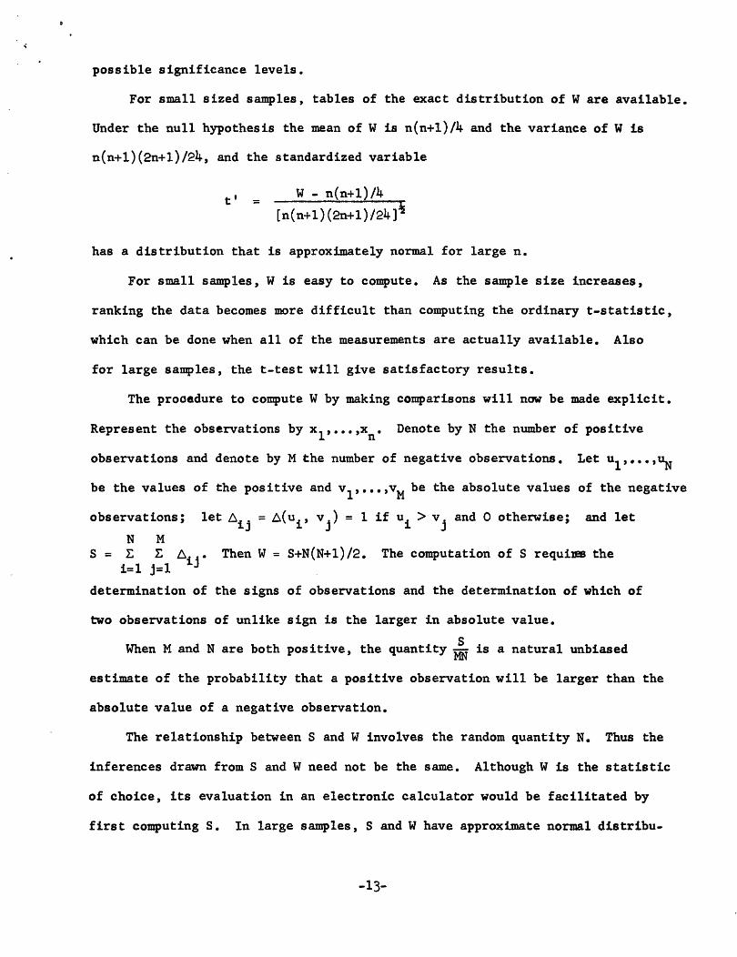
For small sized samples, tables of the exact distribution of Ware available.
Under the null hypothesis the mean of Wis n(n+l)/4 and the variance of Wis
n(n+l)(2n+l)/24, and the standardized variable
t' = W - n(n+l)/4
[n(n+1)(2n+l)/24]i
has a distribution that is approximately normal for large n.
For small samples, Wis easy to compute. As the sample size increases,
ranking the data becomes more difficult than computing the ordinary t-statistic,
which can be done when all of the measurements are actually available. Also
for large samples, the t-test will give satisfactory results.
The procedure to compute W by making comparisons will now be made explicit.
Represent the observations by x1 , ••• ,xn. Denote by N the number of positive
observations and denote by M the number of negative observations. Let u1 , ••• ,°N
be the values of the positive and v1
, ••• ,vM be the absolute values of the negative
observations; let .6ij = .6(ui, vj) = 1 if ui > vj and O otherwise; and let
N M S = E L 6.j. Then W = S+N(N+l)/2. The computation of S requiim the
i=l j=l 1
determination of the signs of observations and the determination of which of
two observations of unlike sign is the larger in absolute value.
s When Mand N are both positive, the quantity MN is a natural unbiased
estimate of the probability that a positive observation will be larger than the
absolute value of a negative observation.
The relationship between Sand W involves the random quantity N. Thus the
inferences drawn from Sand W need not be the same. Although Wis the statistic
of choice, its evaluation in an electronic calculator would be facilitated by
first computing s. In large samples, Sand W have approximate normal distribu-
-13-
.-tions. If the alternative hypothesis is true, the moments, means and variances
of Sand Ware complicated. Except in the case of the sign test, it is usually
difficult to compute the power functions of nonparametric tests. Most state
ments about the power of the W test are based on very small samples, Monte
10/ Carlo results, or asymptotic theory.-
CONFIDENCE INTERVALS FOR A MEDIAN FROM TIIE WILCOXON STATISTIC -------The Wilcoxon test generates confidence intervals for the location parameter
M. 10 The significance level 128
corresponds to rejecting the null hypothesis
when W ~ 25 or W ~ 3. The interval cons.isting of values of M for which
4 ~ W ~ 24 has confidence 10 118 1 -128
= 128
• An examination of the original data
(the ranks are not sufficient) yields for this inte~al all M values between
-1.28 and 4.08. An examination of some trial values of M will help in under
standing this result. Thus if M = 4.2, F has rank 1, G has rank 2, no other
observation has positive rank and W=3, which means this null hypothesis would
be rejected. If M=4, then F has rank 1, G has rank 3, no other observation has
positive rank, and W=4, which means this null hypothesis would be accepted.
RANDOMIZATION TESTS FOR A LOCATION PARAMETER -- -- - ---- ----As a final test for the location parameter, we will consider a randomization
test. Under the null hypothesis the observations are mutually independent and
come from populations symmetric about the median M0 • This includes the cases
where the signed ranks are the basic observations and where the signs are the
basic observations (scoring +1 for a positive observation. and -1 for a negative
observation). Given the absolute values of the differences between the observa-
n tions and M0 , under the null hypothesis there are 2 equally likely possible
assignments of signs to the absolute values. The nonparametric test to be con
sidered rejects large values of the total, T, of the positive observations. 111
The relevant distribution is the conditional distribution of T given the absolute
-14-
values of the observed differences. Using M0 = -.5, for the present data
T = 15.70. There are 13 configurations Gf the signs that will give a value of
T ::. : which is at least this large and another 13 configurations for which T
is 17.52 - 15.70 = 1.82 or smaller; the latter being the lower tail of the
symmetrical distribution of T. Thus the level of significance of the randomiza-
26 tion test on the present data is 128
= .2031. With the test, each multiple of
64 -1 is a possible significance level. The computations for this procedure are
prohibitive except for very small sample sizes. Even with an electronic
calculator this computation is not feasible with more than twenty observations.
A partial solution is to use only some of the assignments of signs (say a random
sample of them) to estimate the conditional distribution of T. T and the
ordinary t-statistic are monotone functions of each other; thus a significance
test based on large values oft is equivalent to one based on large values of T.
The distribution oft under randomization is approximately normal for large
values of n. The normal table can be used to approximate the significance
level oft or of T. Actually, the randomization which occurs in the design of
experiments yields the nonparametric structure discussed here. (Most applications
of the t-test are based on the large sample theory appropriate to the randomiza
tion technique.) The power of the randomization test is approximately the same
as that of the t-test. Hence, when the data are from a normal population, the
tests will have good power. Among nonparametric tests, the randomization tests
are uniformly most powerful for one-sided normal alternatives. (The randomization
test is nonparametric in that the associated level of significance can be
determined exactly for a large class of distributions.)
Finally, confidence intervals can be constructed for M by using the 0
randomization procedure. The procedure is analogous to that used with the
Wilcoxon statistic. 122 The confidence interval with level 128
= .955 is
(-1.107, 4.376).
-15-
Throughout this discussion it is assumed that under the null hypothesis
observations are equally likely to be positive or negative. The Wilcoxon and
randomization procedures assume the distributions are symmetric about~ under
the null hypothesis. These conditions are automatically satisfied in the
following important experimental situation. The observation xi is a difference
y11 - yi2 where yij is the result of applying treatment j to one of a pair of
experimental units. The element of the pair to receive treatment 1 is selected
12/ by a random procedure. -
COMPARISONS OF TESTS FOR A LOCATION PARAMETER ----- - -- - - ---- -----The tests are consistent, i.e., for a particular alternative and large
sample size, each of the tests will have power near one. To compare the large
sample power of the tests, a sequence of alternatives approaching the null
hypothesis is introduced. In particular, let~ be the alternative for experi-
c ment N, and assume~ - M0 = ~ where c is a constant. This framework is
N appealing since larger sample sizes should be used to make finer distinctions. 13/
The efficiency of a test II compared to a test I is defined as the ratio
n1(N) = ----- where n1 and n._1 are the sample sizes yielding the same power
nII(NJ 1
functions for test I and for test II. It is interesting that EI,II does not
depend appreciably on the significance level or the value of c. EI,II does,
however, depend on the distributions of the populations being sampled.
The measure of efficiency EI,II can be used thus: With sample size
n1
(N)[n11
(N)] assume the cost of conducting a test based on test I (II) is
14/ 1InI{N) 11 11n1 (N)[111n11 (N)]. - When 1II~I(N) =
111 ;~t~II:·.is > 1, procedure II
costs less than procedure I, and the two procedures have almost the same power
functions, i.e., procedure II is more economical than procedure I. When
11 EI,II < 1, procedure I is preferred over procedure II ;and when - EI,II = 1,
111
-16-
there is almost no basis for choosing.
The r associated with the sign test can be much smaller than the r's
associated with the Wilcoxon and randomization tests. The r of a particular
procedure can become infinite when there is no experimental technique available
to obtain the necessary data. Thus EI,II is not an absolute measure of efficiency;
it. is meaningful only when costs are taken into consideration and the relevant
alternative hypotheses are clearly specified.
For normal alternatives, where the parameter is the mean:
E - 1 t test, randomization test - ' Et test, Wilcoxon test= 3/~ = .955, and
Et test, sign test= 21~ = •637.
Additional E values can be obtained from
EII,III =
TESTS OF INDEPENDENCE
It has been assumed that the observations are mutually independent and come
from the same distribution (or at least distribution with the same median}. This
assumption can be examined. A procedure for this is based on the number of runs
above and below the (sample) median, the Wald-Wolfowitz run test. For the
present data, scoring 1 for an observation above the median (.75) and O for an
observation below the median, yields the sequence 000111. The order of the
elements in this sequence is the order (A, B, ••• ,G) in which the observations
were made. A run consists of a sequence of like elements whose termini are
either unlike elements or a terminus of the sequence, e.g., 01100110 has 5 runs;
a run of O's of length 1, then a run of l's of length 2, then a run of O's of
length 2, then a run of l's of length 2 and finally a run of O's of length 1.
For the data under consideration there are 2 runs. There is one other sequence
-17-
of 2 runs (111000). 6 There are (3
) = 20 equally likely sequences under the null
hypothesis. For a critical region based on a small number of runs, the present
2 data are significant at the 20 = .1 level. This test has intuitive appeal
for several kinds of alternatives, e.g., a trend for higher measurements to
occur in the latter observations, as with a learning effect.
TOLERANCE INTERVALS
Tolerance intervals are inferences about future observations. They are
confidence intervals for future observations. A form of nonparametric tolerance
(n-2i+l) interval statement asserts that the expected probability is (n+l) that a
future observation will be in the interval (x(i)' x(n-i+l)). Alternatively, when
sampling from a population with distribution function F(x), the expected value
( ) ( ) n-2i+l of F x(n-i+l) - F x(i) is n+l • Thus for the particular data, (-1.96, 6.95)
7-2+1 ( is expected to contain 7+1100% = 75% of the population. The last statement
is a loose use of words of the same kind as saying that an observed confidence
interval has confidence coefficient 95%. Of course, once the data are obtained,
there is no random element left in the problem. In the same way the expected
proportion in this interval depends on the unknown distribution function.
Nevertheless, the loose way of speaking, in a Bayesian framework, is approximately
correct provided the prior distribution is diffuse. 151 )
GOODNESS-OF-FIT TESTS
It is possible to make inferences about the entire distribution with
goodness-of-fit procedures. These procedures can be used to test the hypothesis
that the data came from a particular population or to form confidence belts for
the whole distribution. Two well known procedures used in goodness-of-fit are
based on the chi-square goodness-of-fit statistic and the Kolmogorov-Smirnov
statistic.
TIED OBSERVATIONS
The discussion has presumed that no pairs of observations have the same
-18-
value and that no observation equals MO
• In practice such ties will occur. If
ties are not extensive their consequence will be negligible even if the procedure
based on the assumption of no ties is used. If exact results are required, the
analysis can be performed given the data in the same manner as suggested for
the randomization procedure.
2. Two-Sample Problems
Experiments with two unmatched samples easily allow comparisons between
the sampled populations. With matching, the same kind of comparisons can be as
madeAwith one sample procedures. Usually, however, one sample procedures allow
inferences about absolute quantities, i.e., properties of a single population.
Comparisons arise naturally when considering the relative advantages of two
experimental conditions or two treatments, e.g., a treatment and a control.
Comparisons are advantageous when absolute standards are unknown or are not
available.
Most of the procedures of Section 1 have analogues relevant for comparisons,
the exceptions being tests of randonmess and tolerance intervals. These procedures
can be used for each population separately. With two samples, the central interest
is again on location parameters, in particular, the difference between location
parameters of the two populations is of interest.
This section will be less detailed than Section 1; the emphasis will be
on the kinds of procedures, and on the analogous aspects of these procedures to
the corresponding one-sample procedures. To be specific, let x1 , ••• ,xm be the
observed values in the first sample, and y1 , ••• ,yn be the observed values in
the second sample and let M and M be the corresponding location parameters X y
with f:::. = M -M • y X
ESTIMATION OF DIFFERENCE OF TWO MEANS ---------The difference in the sample averages y-x is often used as a point estimate
-19-
of 6.
When all of the observations are independent and come from normal populations,
this is the maximum-likelihood estimate of 6; if the observations are independent,
this is the Gauss-Markoff estimate; and it is always the least squares estimate.
With the normal assumption, confidence intervals for 6 can be obtained, utilizing
the t-distribution. If the parent populations can have different variances, then
the confidence intervals obtained from the t-distribution will not be exact, i.e.,
they will not have the desired confidence level. Constructing confidence
intervals in this situation has been the subject of much discussion (the
Behrens-Fisher problem). Also, the nonparametric confidence intervals for 6
will not have the prescribed confidence level, unless the two populations differ
in location parameter only.
BROWN-MOOD TESTS AND CONFIDENCE INTERVALS FOR THE DIFFERENCE OF TWO MEDIANS ----- ---- -- -- ----- - -- ----The analogue of the confidence procedure based on signs, i.e., the
Brown-Mood procedure, is constructed in the following manner: let w1 , ••• ,wm+n
be all the observations from the two samples arranged in increasing order, e.g.,
w1 is the smallest observation in both samples; w2 is the second smallest
observation in both samples, etc. Denote by w*, the middle value of thew's,
i.e., w* is the median of the combined sample. (To simplify the discussion, it
will be assumed that m+n is odd, which insures the existence of a middle
observation.) Let m* be the number of w's greater than w*, that came from the
x-population. When the two populations are the same, m* has a hypergeometric
distribution, i.e.,
Pr(m*=k) = where N=(m+n-1)/2.
Thus, a nonparametric test of the hypothesis that the two populations are the
same, specifically that 6=0, is based on the distribution of m*, i.e., reject
the null hypothesis when m* is either too large or too small, computing the
-20-
probabilities from the above distribution. To obtain confidence intervals:
replace the x-sample with xi= x1 + 6(i=l, ••• ,m), form a new sequence out of
the x'values and they values analogous to thew sequence and call it thew'
sequence; compute the median w'* and m'* and see if the null hypothesis of no
difference between the x' and y population can be accepted; if it is accepted
then 6 is in the confidence interval, and if it is rejected then 6 is not in
the confidence interval. (A graphical procedure can be used.)
WILCOXON TWO-SAMPLE TESTS AND CONFIDENCE INTERVALS
The analogue to the Wilcoxon procedure is to assign ranks {a set of
conventional numbers) to thew's, i.e., w1 is given rank 1; w2 is given rank
2, etc •• 161 The test statistic is the sum of the ranks of those w's which came
from the x-population,. When the two populations are identical except for
location, this test statistic will be nonparametric; its distribution under
the hypothesis will not depend on the underlying common distribution. The
null hypothesis is rejected when the statistic is excessive in the appropriate
directions. This procedure is called the two-sample Wilcoxon test or the
Mann-Whitney test.
The Wilcoxon procedure for two samples can be used ~f if is possible to
compare each observation from the x-population with each observation from the
y-population. The Mann-Whitney version of the Wilcoxon statistic (it is a
non random linear function of the Wilcoxon statistic) is the number of times
an observation from they-population exceeds an observation from the x-p9pulation.
When this number is divided by nm, it becomes an unbiased estimate of Pr(Y > X),
i.e., the probability that a randomly selected y will be large~ than a randomly
selected x. This parameter has many interpretations and uses, e.g., if stresses
(one from each of two populations) are brought together by random selection,
it is the probability that the stress from one population will exceed that of
the other (the system will function). In estimating this parameter, it is not
-21-
necessary to assume that the two populations differ in location only.
RANDOMIZATION TESTS AND CONFIDENCE INTERVALS
FOR THE DIFFERENCE OF TWO LOCATION PARAMETERS -- -- ----- - -- ----- ------The randomization procedure is based on the conditional distribution of
the sum of the observations in the x-sample given thew sequence, when each
selection of m of the values from thew sequence is considered equally likely.
There are (m+n) such possible selections. The sum of the observations in the m
x-sample is an increasing function of the usual t-statistic. The importance of
the randomization procedure is that it gives a method for handling any problem;
for most sets of data, it is practically the same as the optimal procedures for
the parametric situation (normal); yet it has exact nonparametric properties.
COMPARISONS OF SCALE PARAMETERS ------ -- --- -----To compare spread, or scale, parameters, the observations can be ranked in
terms of their distances from w*, the combined sample median. If the populations
have the same median, the sum of ranks corresponding to the x-sample is a useful
statistic. When the populations are identical, this sum of ranks has a distri
bution which does not depend on the underlying distribution. If the x-population
is more (less) spread out than they-population, then this sum will tend to be
larger (smaller) than under the null hypothesis. When the null hypothesis does
not include the assumption that both populations have the same median, the
observations can be replaced in each sample by their deviations from their
medians, and then thew-sequence can be formed from the deviations in both
samples. Proceeding from there, the ranking procedures will not be exactly
nonparametric but should yield results with significance and confidence levels
near the nominal levels.
3. Other Problems
Many other problems and techniques have been presented for the one and two
-22-
sample situations, and many other situations have been discussed. A selection
of these topics will be mentioned.
SEQUENTIAL PROCEDURES
Sequential experiments often save money or time in experimentation. The
sign procedure is easily put into a sequential form. Sequential forms of other
nonparametric procedures are being investigated.
INVARIANCE, SUFFICIENCY, AND COMPLETENESS
Such concepts as invariant statistics, sufficient statistics, and complet,
statistics arise in nonparametric theory. In the two-sample problem, the ranks
of the first sample considered as an entity, have these properties when only
comparisons are obtainable between the observations of the x- and y-samples or
if the measurement scheme is unique only up to monotone transformations. (The
measurement scheme is unique up to monotone transformations if there is no
compelling reason why particular scales of measurement should be used. Non
parametric confidence intervals (for percentiles} are invariant under monotone
transformations. If a nonparametric confidence interval has been formed for a
location parameter, the interval with end points cubed will be the confidence
interval which would have been obtained if the original observations had been
replaced by their cubes. Maximum likelihood estimation procedures have a
similar property.}
MULTIVARIATE ANALYSIS
Although correlation techniques have not been described in this article,
it is important to realize that Spearman's rank correlation procedure acted as
a stimulus for research in nonparametric analysis. Problems such as partial
correlation and multiple correlation have not received adequate nonparametric
treatment. For these more complicated problems, the most useful available
techniques are associated with the analysis of multi-dimensional contingency
tables.
-23-
MULTIPLE USES OF A STATISTIC ---- -- - - -----Often, a particular test statistic can be used in widely different contexts.
Thus the total number of runs, Wald-Wolfowitz test, discussed above as a test
of randomness, was originally proposed as a test of goodness-of-fit. (It is
not recommended as a goodness-of-fit test because more powerful tests, such as
the Kolmogorov-Smirnov test, are available.)
MULTIPLE USES OF A WORD ----------The same words are often used for different procedures. Thus rank
correlation does not specifically refer to the Spearman rank correlation which
is an analogue to the standard correlation coefficient. It can refer to Kendall's
tau. Many kinds of runs have been discussed in the literature, e.g., runs up
and down; runs of different lengths; runs above and below a population median.
These statistics have different uses and may have different distributions.
ANALYSIS OF VARIANCE (ANALOGUES)
A substantial body of nonparametric procedures has been proposed for the
analysis of experiments involving several populations. Analogues have been
devised for the standard analysis of variance procedures. One such analogue
involves the ranking of all of the measurements in the several samples, and
then performing an analysis of variance of rank data (Kruskal-Wallis procedure).
Another procedure involves each of several judges ranking all populations
{the Friedman-Kendall technique).
DECISION THEORY
Other decision procedures than estimation and testing have not received
extensive nonparametric attention. An example, however, is the Mosteller
procedure of deciding whether or not one of several populations has shifted,
say to the right. It can be thought of as a multiple decision problem since
if one rejects the null hypothesis (the populations are the same), it is natural
to decide that the "largest" sample comes from the "largest" population. (Most
-24-
::
users of statistics, when rejecting a null hypothesis with a two sided test,
act as if the parameter is in the direction of the observed difference. 171 )
Analysis of the several Wilcoxon statistics which can be obtained by considering
pairs of samples when observations are obtained from several populations will
lead to multiple decision procedures.
4. References
The extensive literature of nonparametric statistics is indexed in the
bibliography of Savage (1962). Detailed information for applying many non
parametric procedures has been given by Siegel (1956) and Walsh (1962). The
advanced mathematical theory of nonparametric statistica has been outlined
by Fraser (1957) and Lehmann (1959).
Fraser, Donald A. S., Non-parametric Methods in Statistics; New York, Wiley, (1957)0
Lehmann, E. L., Testing Statistical Hypotheses; New York, Wiley, (1959).
Savage, I. Richard, Bibliography of Nonparametric Statistics; Cambridge, Mass.,
Harvard University Press, (1962).
Siegel, Sidney, Nonparametric Statistics for the Behavioral Sciences, New York,
McGraw-Hill, (1956).
Walsh, John E., Handbook of Nonparametric Statistics: Investigation of
Randonmess, Moments, Percentiles, and Distributions, New York, Van Nostrand,
5.
1/
2/
(1962). I'\
Footnotes
The general plan of writing is to decrease detail as we move to latter
parts of the paper. In particular such topics as "continuity corrections"
and "ties" are not mentioned each time they could be relevanto
The considerations of this sentence (in the text) are of course interrelatedo
It is clear that a good experiment and a good analysis will be able to
accomplish several things. An item such as costs,of course, can refer to
-25-
a 1i
a multiplicity of things, e.g., cost of conducting the experiment, cost
of analysis, or costs of making incorrect decisions. The audience is often
not of a connnon mind and thus CQmpromises in presentations might be required.
The emphasis is on the fact that the good application of statistics is
seldom a clear cut use of text book directions without the consideration
of many related matters.
:J/ Assume that 0 has a prior density function, p(e). Then the posterior density
of e given the sample data is of the following form
Cp(B)exp - n2 (x-0)2
2a
where C does not depend on 8 and xis the average of then observations.
If n/a2 is large the exponential term of this expression will be very
small except for values of e near x. Then the maximizing value of 8 must
be near x unless p(8) has a very large peak away from x. The diffuseness
of the distribution of 0 is intuitively associated with the lack of high
peaks in p(e). Under similar circumstances xis near the posterior mean
of e. In the Bayesian framework, one would not report an estimate but
would either give the posterior distribution of 8 or recoDD11end a decision.
4/ The method of least squares is an algebraic computing device.. The·.1east
squares estimates can be computed without making any .probabilistic
assumptions about the source of the data. It is important in statistical
inference since under specified conditions the least squares estimates have
good (in a probabilistic sense) properties. In particular, the least squares
estimates are often the minimum variance unbiased estimates based on linear
functions of the data, i.e., the Gauss-Markoff estimates.
'2_/
6/
A population is symmetric about a point M if the probability of an observation
more than X units below Mis the same as the probability of an oliservation·
more than X units above M for each X > O.
Generalities are likely to obscure a good part of detail. Thus if one
really had a very large sample and were interested in the population median,
it might be best to work with the sample median even if you were quite sure
that population was nearly normal. The sample median is sure to do the job
-26-
8/
10/
and if the sample size is large there is not DDJch possible loss of in
formation by using the median instead of the mean. On the other hand even
if you are sure about the population being near normal, the slight deviation
might cause the mean and median not to be the same so that even with a
large sample one could not get covergence to the correct answer using the
mean.
A coDDI10n practice is to select a level of significance before the experiment
is conducted and then to report whether or not the sample was significant
at that level. Here, the report states the smallest level of significance
at which the obtained data would be found significant.
Here and in several later places, it is sUressed that nonparametric procedures
often do not require actual measurements, i.e., comparisons of individuals
with norms or with each other might be sufficient. Occasionally, there is
a real cost savings in ma.king the comparisons rather than the measurements,
e.g., using go-no-go gauges in quality control rather than actual measure
ments. In the social sciences, the precise thing to measure is often very
obscure and at best one can make comparisons.
The irrelevance of which signed rank is associated with which individual,
depends on the assumptions that the individual scores are independently
distributed and that each individual has the same probability of exceeding
the null value of the parameter. A discussion of tests of these hypotheses
is indicated in TESTS OF INDEPENDENCE later in the text.
When n, the sample size, is very small, say less than 6, it is sometimes
possible to compute the value of the power function by the analytic
evaluation of integrals or the numerical evaluation of integrals in an
electronic computero For intermediate sized samples Monte Carlo experiments
are useful. That is, one draws a sample from the population of interest
and evaluates the test statistic. This process is done many times. The
resulting sample of values of the test statistic is used to approximate the
distribution of the test statistic. Usually the experiment is performed in
an electronic computer. For large samples, it is known that the test
statistic has approximately a normal distribution with mean and variance
determined by the hypothesis and the sample size. A table of the normal
distribution can then be used to evaluate the approximate probability of
the test statistic being in a specified range.
-27-
11/
12/
13/
14/
'J:§.I
Large values of Tare used when the alternative hypothesis asserts that
the median is larger than M0• Small values of T would be used if the
alternative asserted the median was less than~· If a two sided alternative
is under consideration, the null hypothesis would be rejected for either
excessively large or small values of T.
It is being assumed that the values of the yij's are not affected by the
treatments being used. Thus yij represents the untreated value of the
individual plus measurement error. If both treatments have the same effect
the model will still be applicable.
In this discussion "N" indicates the element in a sequence of experimental
situations. As N increases the situation approaches the null hypothesis.
In the next paragraph of the text, two sequences of tests are described.
There is an element in each test sequence for each experimental condition.
In particular the experimental situation (with other conditions) determines
the sample sizes for each test. The other conditions being that the two
tests have (approximately) the same significance level :·. :regardless of the
sample sizes and that for each experimental situation the tests have
(approximately) the same power. Alternative useful analyses requite the
significance level to decrease as more data are obtained or, the matching
of the slopes of the power functions at the null hypothesis, etc.
The r's measure the costs of obtaining a single observation to be used in
the computation of the relevant test statistics.
The statement is misleading in that the research required to give a detailed
:.d·aacription of "diffuse" and "approximately" has not been performed.
Another interesting scheme is to replace w1 with the expected value of the
smallest observation in a sample of size m+n from a normal distribution
with mean O and variance 1, replace w2 with the expected value of the second
amalleat observation from the same population, etc. The sum of the expected
values corresponding to the x-sample has properties similar to the t-atatistic
when the two samples in fact come from normal distributions differing in
location only,
rJ./ Such behavior i1 not in agreement with the 1trict logic of the NeymanPear,on theory of teata of hnotheaaa. 'rh&t theory, however, ia not action oriented. 'l'he actual behavior ii con.ail tent with a Baya1ian framework for tliia problem,