87
Nonparametric testing for exogeneity with discrete regressors and instruments Katarzyna Bech and Grant Hillier Warsaw School of Economics and University of Southampton July 8, 2016 1/28
| Date post: | 12-Apr-2017 |
| Category: |
Economy & Finance |
| Upload: | grape |
| View: | 43 times |
| Download: | 0 times |

Nonparametric testing for exogeneity with discreteregressors and instruments
Katarzyna Bech and Grant Hillier
Warsaw School of Economicsand
University of Southampton
July 8, 2016
1/28

Outline
1 Motivation.
2 Simplest nonparametric additive error model- setup, identication,estimation.
3 Two test statistics and critical values computation.4 Generalization to several variables of each type- tested, exogenous,instrument.
5 Applications: Card (1995) and Angrist and Krueger (1991).
2/28

Outline
1 Motivation.2 Simplest nonparametric additive error model- setup, identication,estimation.
3 Two test statistics and critical values computation.
4 Generalization to several variables of each type- tested, exogenous,instrument.
5 Applications: Card (1995) and Angrist and Krueger (1991).
2/28

Outline
1 Motivation.2 Simplest nonparametric additive error model- setup, identication,estimation.
3 Two test statistics and critical values computation.4 Generalization to several variables of each type- tested, exogenous,instrument.
5 Applications: Card (1995) and Angrist and Krueger (1991).
2/28

Outline
1 Motivation.2 Simplest nonparametric additive error model- setup, identication,estimation.
3 Two test statistics and critical values computation.4 Generalization to several variables of each type- tested, exogenous,instrument.
5 Applications: Card (1995) and Angrist and Krueger (1991).
2/28

Motivation
Endogeneity is one of the common problems in econometric models.
In nonparametric models with discrete regressors and instruments, thepresence of endogenous regressors produces bias (in the identiedcase) or non-existance of any consistent estimator (in the partiallyidentied case).
IV for nonparametric models with discrete regressors: Das (2005) andFlorens and Malavolti (2003).
Nonparametric testing for exogeneity with continuous regressors:Blundell and Horowitz (2007), Lavergne and Patilea (2008) amongothers.
3/28

Motivation
Endogeneity is one of the common problems in econometric models.In nonparametric models with discrete regressors and instruments, thepresence of endogenous regressors produces bias (in the identiedcase) or non-existance of any consistent estimator (in the partiallyidentied case).
IV for nonparametric models with discrete regressors: Das (2005) andFlorens and Malavolti (2003).
Nonparametric testing for exogeneity with continuous regressors:Blundell and Horowitz (2007), Lavergne and Patilea (2008) amongothers.
3/28

Simple model
Nonparametric additive error model
Y = h(X ) + ε
E [εjZ = zj ] = 0, 8j
where we have i .i .d . data (x si , ysi , z
si ) on (X ,Y ,Z ), and
Y is a continuous scalar dependent variable,
X is a single discrete regressor with support fxk , k = 1, ...,Kg, thatmay be endogenous, with associated probabilities pk > 0,
Z is a discrete instrumental variable with support fzj , j = 1, ..., Jg,with associated probabilities qj > 0.
4/28

Hypothesis of interest
Null hypothesis (exogeneity):
H0 : E [εjX = xk ] = 0, k = 1, ..,K .
Under the null, h() can be consistently estimated using standardnonparametric techniques.
Under the alternative, the IV solution to endogeneity only possibleunder point identication.
5/28

Hypothesis of interest
Null hypothesis (exogeneity):
H0 : E [εjX = xk ] = 0, k = 1, ..,K .
Under the null, h() can be consistently estimated using standardnonparametric techniques.
Under the alternative, the IV solution to endogeneity only possibleunder point identication.
5/28

Hypothesis of interest
Null hypothesis (exogeneity):
H0 : E [εjX = xk ] = 0, k = 1, ..,K .
Under the null, h() can be consistently estimated using standardnonparametric techniques.
Under the alternative, the IV solution to endogeneity only possibleunder point identication.
5/28

Identication
Since
Y =K
∑k=1
h(xk )I (X = xk ) + ε,
the conditional expectation of Y given Z = zj is
E [Y jZ = zj ] =K
∑k=1
Pr[X = xk ,Z = zj ]h(xk ).
) the instrument Z supplies the equations
π = Πβ,
where βk = h(xk ),πj = E [Y jZ = zj ],Πjk = P [X = xk jZ = zj ].h() is identied at ALL support points of X i¤ J K .
6/28

Identication
Since
Y =K
∑k=1
h(xk )I (X = xk ) + ε,
the conditional expectation of Y given Z = zj is
E [Y jZ = zj ] =K
∑k=1
Pr[X = xk ,Z = zj ]h(xk ).
) the instrument Z supplies the equations
π = Πβ,
where βk = h(xk ),πj = E [Y jZ = zj ],Πjk = P [X = xk jZ = zj ].
h() is identied at ALL support points of X i¤ J K .
6/28

Identication
Since
Y =K
∑k=1
h(xk )I (X = xk ) + ε,
the conditional expectation of Y given Z = zj is
E [Y jZ = zj ] =K
∑k=1
Pr[X = xk ,Z = zj ]h(xk ).
) the instrument Z supplies the equations
π = Πβ,
where βk = h(xk ),πj = E [Y jZ = zj ],Πjk = P [X = xk jZ = zj ].h() is identied at ALL support points of X i¤ J K .
6/28

Identication when J<K
h() is partially identied when J < K :
Theorem 1Let L(β) = c 0β be a linear functional of the elements of β. Whenrank(Π) = J < K , the following are true:(1) for any c orthogonal to the null space of Π, L(β) is point-identied;the dimension of this set is J.(2) for c not orthogonal to the null space of Π, L(β) is completelyunconstrained; the dimension of this set is K J.
That is: when J < K , some linear functionals are point-identied,some completely arbitrary (not even set-identied!).Point-identiability of L(β) can be tested (for a given choice of c):
Gn = nc 02 c 01Π1
1 Π2V1P
c 02 c 01Π1
1 Π20 !d χ2KJ .
7/28

Identication when J<K
h() is partially identied when J < K :
Theorem 1Let L(β) = c 0β be a linear functional of the elements of β. Whenrank(Π) = J < K , the following are true:(1) for any c orthogonal to the null space of Π, L(β) is point-identied;the dimension of this set is J.(2) for c not orthogonal to the null space of Π, L(β) is completelyunconstrained; the dimension of this set is K J.
That is: when J < K , some linear functionals are point-identied,some completely arbitrary (not even set-identied!).
Point-identiability of L(β) can be tested (for a given choice of c):
Gn = nc 02 c 01Π1
1 Π2V1P
c 02 c 01Π1
1 Π20 !d χ2KJ .
7/28

Identication when J<K
h() is partially identied when J < K :
Theorem 1Let L(β) = c 0β be a linear functional of the elements of β. Whenrank(Π) = J < K , the following are true:(1) for any c orthogonal to the null space of Π, L(β) is point-identied;the dimension of this set is J.(2) for c not orthogonal to the null space of Π, L(β) is completelyunconstrained; the dimension of this set is K J.
That is: when J < K , some linear functionals are point-identied,some completely arbitrary (not even set-identied!).Point-identiability of L(β) can be tested (for a given choice of c):
Gn = nc 02 c 01Π1
1 Π2V1P
c 02 c 01Π1
1 Π20 !d χ2KJ .
7/28

Linear Model Setup
We dene the (0, 1) matrix LX (nK ) with elements(LX )ik = I (x si = xk ). Likewise LZ (n J). Then, H0 says:
y = LX β+ ε, E [εjX = xk ] = 08k.
β can be consistently estimated by OLS under exogeneity:
bβ = (L0X LX )1L0X y =0BB@
∑ni=1 yi I (x
si =x1)
∑ni=1 I (x
si =x1)
...∑ni=1 yi I (x
si =xK )
∑ni=1 I (x
si =xK )
1CCA .
Theorem 2
If X is exogenous then the nonparametric (OLS) estimator bβ is consistentand p
nbβ β
!d N
0, σ2D1X
,
where DX is diag(pk ).
8/28

Linear Model Setup
We dene the (0, 1) matrix LX (nK ) with elements(LX )ik = I (x si = xk ). Likewise LZ (n J). Then, H0 says:
y = LX β+ ε, E [εjX = xk ] = 08k.β can be consistently estimated by OLS under exogeneity:
bβ = (L0X LX )1L0X y =0BB@
∑ni=1 yi I (x
si =x1)
∑ni=1 I (x
si =x1)
...∑ni=1 yi I (x
si =xK )
∑ni=1 I (x
si =xK )
1CCA .Theorem 2
If X is exogenous then the nonparametric (OLS) estimator bβ is consistentand p
nbβ β
!d N
0, σ2D1X
,
where DX is diag(pk ).
8/28

Linear Model Setup
or by IV (with LZ as instruments) under endogeneity, when J K :bβIV = L0XPLZ LX 1 L0XPLZ y .
Theorem 3
Under assumptions above, the IV estimator bβIV is consistent andpnbβIV β
!d N
0, σ2
P 0D1Z P
1,
where P is a matrix of joint probabilities with elements
pjk = Pr [Z = zj ,X = xk ] ; j = 1, ..., J; k = 1, ...,K
and DZ is diag(qj ).
BUT no consistent estimator exists for K J linear functionals if X isendogenous and J < K .
9/28

Linear Model Setup
or by IV (with LZ as instruments) under endogeneity, when J K :bβIV = L0XPLZ LX 1 L0XPLZ y .Theorem 3
Under assumptions above, the IV estimator bβIV is consistent andpnbβIV β
!d N
0, σ2
P 0D1Z P
1,
where P is a matrix of joint probabilities with elements
pjk = Pr [Z = zj ,X = xk ] ; j = 1, ..., J; k = 1, ...,K
and DZ is diag(qj ).
BUT no consistent estimator exists for K J linear functionals if X isendogenous and J < K .
9/28

Test for exogeneity
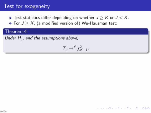
Test statistics di¤er depending on whether J K or J < K .
For J K , (a modied version of) Wu-Hausman test:
Theorem 4Under H0, and the assumptions above,
Tn !d χ2K1.
Theorem 5Under the sequence of local alternatives, and the assumptions above, thetest statistic
Tn !d Gamma (β,λ, θ) ,
with the shape parameter α = K12 , the scale parameter θ = 2 σ2
σ2 and thenoncentrality parameter λ = 2δ2, where
δ2 =ξ 0Σ111 ξ
σ2.
10/28

Test for exogeneity
Test statistics di¤er depending on whether J K or J < K .For J K , (a modied version of) Wu-Hausman test:
Theorem 4Under H0, and the assumptions above,
Tn !d χ2K1.
Theorem 5Under the sequence of local alternatives, and the assumptions above, thetest statistic
Tn !d Gamma (β,λ, θ) ,
with the shape parameter α = K12 , the scale parameter θ = 2 σ2
σ2 and thenoncentrality parameter λ = 2δ2, where
δ2 =ξ 0Σ111 ξ
σ2.
10/28

Test for exogeneity
For J < K , the test is based on the two SSE:
Unrestricted: in the model y = LX β+ ε, i.e., y 0MLX y , andRestricted: minimising the SSE in this model subject to π = Πβ.
Test statistic:
Rn =y 0MLX LZ (L
0ZPLX LZ )
1 L0ZMLX yn1y 0MLX y
.
11/28

Test for exogeneity
For J < K , the test is based on the two SSE:
Unrestricted: in the model y = LX β+ ε, i.e., y 0MLX y , and
Restricted: minimising the SSE in this model subject to π = Πβ.
Test statistic:
Rn =y 0MLX LZ (L
0ZPLX LZ )
1 L0ZMLX yn1y 0MLX y
.
11/28

Test for exogeneity
For J < K , the test is based on the two SSE:
Unrestricted: in the model y = LX β+ ε, i.e., y 0MLX y , andRestricted: minimising the SSE in this model subject to π = Πβ.
Test statistic:
Rn =y 0MLX LZ (L
0ZPLX LZ )
1 L0ZMLX yn1y 0MLX y
.
11/28

Test for exogeneity
For J < K , the test is based on the two SSE:
Unrestricted: in the model y = LX β+ ε, i.e., y 0MLX y , andRestricted: minimising the SSE in this model subject to π = Πβ.
Test statistic:
Rn =y 0MLX LZ (L
0ZPLX LZ )
1 L0ZMLX yn1y 0MLX y
.
11/28

Test for exogeneity
Theorem 6
Under H0 and the assumptions above,
Rn !d z 0Ω1z J1∑j=1
ωjχ2j (1)
where z N(0,Σ), with Σ as dened above,
Ω := C 0J (PD1X P 0 pZ p0Z )CJ ,
and the ωj are positive eigenvalues satisfying
det[ΣωΩ] = 0
with the χ2j (1) variables independent copies of a χ21 random variable.
12/28

Critical value computation
using consistent estimates of bωj , simulate the distribution of
∑(J1)j=1 bωjχ
2j (1) to get the appropriate 1 α quantiles,
simulate the quadratic form z 0 bΩ1z , with z N(0, bΣ) and computethe quantiles,
approximate by the distribution of aχ2(v ) + b, choosing (a, b, v) tomatch the rst three cumulants.
13/28

Generalizations: model with two discrete regressors
Y = h(W ,X ) + ε
E [εjZ = zj ,W = wd ] = 0, 8j , d
We dene LWX (nDK ) with elements(LWX )i ,dk = I (W = wd )I (X = xk ). Likewise LWZ (nDJ), and H0says:
y = LWX β+ ε,E [εjW = wd ,X = xk ] = 08d , k.
14/28

Structure of regression matrix
LWX is a permutation of the rows of2664L1X 0 0 00 L2X 0 00 0 00 0 0 LDX
3775
Observations corresponding to LdX all have W = wd , and rowsidentify which values of X occur where.
Similarly for LWZ .
We assume that all possible combinations of K support points of X , Jsupport points of Z and D support points of W occur in the sample.
15/28

Structure of regression matrix
LWX is a permutation of the rows of2664L1X 0 0 00 L2X 0 00 0 00 0 0 LDX
3775Observations corresponding to LdX all have W = wd , and rowsidentify which values of X occur where.
Similarly for LWZ .
We assume that all possible combinations of K support points of X , Jsupport points of Z and D support points of W occur in the sample.
15/28

Identication in general model
The vector with elements h(wd , xk ) can be split into D K 1vectors, with component vectors hd (xk ), say, one for each wd .
So we have D problems of the same type as the case with W absent.[Split y into D subvectors yd ]
The instrument is valid for each subsample.
For h to be point-identied, each hd must be, so the condition isagain J K .
16/28

Most general model
Now assume several variables of each type:X1, ..,XR ,W1, ..,WU ,Z1, ..,ZT , with respective supports ofdimensions Kr ,Su , Jt .
We want to test the joint endogeneity of (X1, ..,XR ) .
Label combinations of support points thus:
xα = (xα1 , .., xαR ), 1 αr Kr ,wβ = (wβ1
, ..,wβS), 1 βu Su ,
zγ = (zγ1 , .., zγT ), 1 γt Jt
Order the sequences lexicographically.
Indistinguishable from the case of one variable of each type, exceptthat
J = ΠTt=1Jt , K = ΠR
r=1Kr , S = ΠUu=1Su .
17/28

In particular - Identication
The N&S condition remains that J K , but with J and K dened asproducts of the Jt and Kr .
BUT note:
There is NO requirement that there should be at least as manyinstruments as endogenous variables (T R);All that is needed is J K .Of course: more instruments increases J = ΠT
t=1Jt .
18/28

In particular - Identication
The N&S condition remains that J K , but with J and K dened asproducts of the Jt and Kr .
BUT note:
There is NO requirement that there should be at least as manyinstruments as endogenous variables (T R);
All that is needed is J K .Of course: more instruments increases J = ΠT
t=1Jt .
18/28

In particular - Identication
The N&S condition remains that J K , but with J and K dened asproducts of the Jt and Kr .
BUT note:
There is NO requirement that there should be at least as manyinstruments as endogenous variables (T R);All that is needed is J K .
Of course: more instruments increases J = ΠTt=1Jt .
18/28

In particular - Identication
The N&S condition remains that J K , but with J and K dened asproducts of the Jt and Kr .
BUT note:
There is NO requirement that there should be at least as manyinstruments as endogenous variables (T R);All that is needed is J K .Of course: more instruments increases J = ΠT
t=1Jt .
18/28

Applications motivation
There are many published applications, where discrete endogenousregressor is instrumented by a variable with insu¢ cient support, e.g.Card (1995), Angrist and Krueger (1991), Bronars and Grogger(1994), Lochner and Moretti (2004).
The point identication is achieved by assuming a parametric (linear)specication.
Parametric vs. nonparametric specication testing (e.g. Horowitz(2006)) not possible in this case.
19/28

Application- Card (1995) on returns to schooling
We are interested in the relationship between individuals wage Y andeducation X (in the presence of exogenous covariates W ) in
Y = h(X ,W ) + ε.
Card (1995) treats education as endogenous and estimates
ln(wagei ) = β0 + β1Xi +S
∑s=1
γsWsi + εi
by 2SLS using a binary instrument Z , which takes value 1 if there is acollege in the neighbourhood, 0 otherwise. The point identication isachieved by imposing the parametric (linear) specication, that is nottestable.
20/28

Data
The dataset consists of 3010 observations from the NationalLongitudinal Survey of Young Men.
The (sample) support of education variable consists of K = 18di¤erent values, and for a binary instrument: J = 2.
Data limitation: the more exogenous covariates, the less likely it is toget observations for all possible combinations of the support points.
Educational levels (K = 4): less than high school, high school, somecollege, post-college education.
Potential labour market experience levels: low and high.
21/28

Results
Covariates Rn cv .1 cv .2 cv .3 α
Educ 1.765 0.239 0.232 0.238 1%0.136 0.132 0.138 5%0.094 0.096 0.097 10%
Educ*, Exp* 4.147 1.221 1.259 1.217 1%0.715 0.696 0.719 5%0.511 0.500 0.515 10%
Educ*, Exp*, Race 3.572 1.771 1.692 1.688 1%1.107 1.131 1.108 5%0.849 0.871 0.860 10%
Educ*, Exp*, Race, SMSA 2.955 2.382 2.330 2.415 1%1.702 1.679 1.735 5%1.399 1.365 1.430 10%
22/28

Outcome
Education is endogenous, whatever the specication of the W 0s.
So: linearity is not testable, because no consistent estimator for h()Some linear functionals of interest may be - use the test above tocheck.
Can consistently estimate an identied linear combination.
23/28

Outcome
Education is endogenous, whatever the specication of the W 0s.
So: linearity is not testable, because no consistent estimator for h()
Some linear functionals of interest may be - use the test above tocheck.
Can consistently estimate an identied linear combination.
23/28

Outcome
Education is endogenous, whatever the specication of the W 0s.
So: linearity is not testable, because no consistent estimator for h()Some linear functionals of interest may be - use the test above tocheck.
Can consistently estimate an identied linear combination.
23/28

Outcome
Education is endogenous, whatever the specication of the W 0s.
So: linearity is not testable, because no consistent estimator for h()Some linear functionals of interest may be - use the test above tocheck.
Can consistently estimate an identied linear combination.
23/28

Testing for point-identiability of linear functionals
As J = 2, linear functionals of only 2 parameters might be pointidentied, eg. the di¤erence in earnings across di¤erent years ofeducation.
linear combination Gn bL(β) Cheshers boundsh(3) h(2) 0.1356 0.0040 -h(7) h(6) 1.9332 0.1017 (0.0365, 0.2895)h(8) h(7) 0.1494 0.2395 (0.1732; 0.352)h(9) h(8) 26.5527 - (0.2742; 0.1334)h(10) h(9) 75.2217 - -h(11) h(10) 4.7003 0.1317 (0.057; 0.3187)h(14) h(13) 61.5525 - -h(17) h(16) 10.7344 -0.1900 -h(18) h(17) 74.1413 - -
24/28

Application- Angrist and Krueger (1991) on returns toschooling
Angrist and Krueger (1991) estimate
ln(wagei ) = βXi +∑c
δcYci +S
∑s=1
γsWsi + εi
by 2SLS using quarter of birth as an instrument for (assumed)endogenous education.
Data: 1980 Census, split into 1930-1939 cohort (40-49 year-old men)and 1940-1949 cohort (30-39 year-old men).
Now, K = 21 and J = 4.
25/28

Results: 1930s cohort
critical valuesRn 1% 5% 10%
1930 0.645 17.144 11.026 8.4331931 1.000 19.806 12.614 9.5821932 10.843 21.541 14.313 11.1841933 2.385 18.980 12.685 9.9521934 6.498 25.674 16.824 13.0251935 2.728 20.451 13.374 10.3401936 10.990 29.102 18.465 13.9801937 1.614 13.467 9.032 7.1011938 1.344 22.932 15.107 11.7371939 9.649 22.130 14.837 11.664
full cohort 38.044 85.933 72.138 65.465
26/28

Results: 1940s cohort
critical valuesRn 1% 5% 10%
1940 3.528 24.137 15.704 12.0961941 18.143 24.733 16.005* 12.286*1942 6.517 34.282 21.810 16.5351943 99.840 55.818* 35.712* 27.202*1944 22.665 39.214 24.860 18.823*1945 31.736 26.623* 17.705* 13.847*1946 17.181 23.478 15.183* 11.642*1947 22.803 33.000 21.830* 17.012*1948 34.116 46.991 29.790* 22.552*1949 32.952 36.445 23.627* 18.168*
full cohort 278.703 138.344* 114.551* 103.182*
27/28

To conlude...
we propose consistent nonparametric exogeneity test(s) applicable inmodels with discrete regressors,
the tests conrm endogeneity of education variable in some classicapplied work, but
suggest that linearity of these models might be a bold assumption;
we suggest a nonparametric approach, or nding instruments withmore support points!
THE END
28/28


