Nonparametric Tests for Common Values

In First-Price Sealed-Bid Auctions

Philip A. Haile† Han Hong‡ Matthew Shum§

September 24, 2003

preliminary

Abstract

We develop tests for common values at rst-price sealed-bid auctions. Our tests arenonparametric, require observation only of the bids submitted at each auction, andare based on the fact that the “winner’s curse” arises only in common value auctions.The tests build on recently developed methods for using observed bids to estimateeach bidder’s conditional expectation of the value of winning the auction. Equilibriumbehavior implies that in a private values auction these expectations are invariant to thenumber of opponents each bidder faces, while with common values they are decreasing inthe number of opponents. This distinction forms the basis of our tests. We consider bothexogenous and endogenous variation in the number of bidders. Monte Carlo experimentsshow that our tests can perform well in samples of moderate sizes. We apply our teststo two di erent types of U.S. Forest Service timber auctions and nd little evidence ofcommon values.

Keywords: rst-price auctions, common values, private values, nonparametric testing,winner’s curse, stochastic dominance, subsampling, endogenous participation, timberauctions

We thank Don Andrews, Steve Berry, Ali Hortacsu, Tong Li, Harry Paarsch, Isabelle Perrigne, RobPorter, Quang Vuong, seminar participants at the Tow conference in Iowa, SITE, the World Congress of theEconometric Society in Seattle, and several universities for insightful comments. We thank Hai Che, KunHuang, and Grigory Kosenok for research assistance. We thank the NSF, SSHRC and Sloan Foundation fornancial support.†Department of Economics, Yale University, P.O. Box 208264, New Haven, CT 06520,

philip.haile@yale.edu‡Department of Economics, Duke University, P.O. Box 90097, Durham, NC 27708, hanhong@duke.edu§Department of Economics, Johns Hopkins University, 3400 N. Charles St., Baltimore, MD 21218,

mshum@jhu.edu.

1

1 Introduction

At least since the in uential work of Hendricks and Porter (1988), studies of auction data

have played an important role in demonstrating the empirical relevance of economic models

of strategic interaction between agents with asymmetric information. However, a funda-

mental issue remains unresolved: how to choose between private and common values models

of bidders’ information. In a common values auction, information about the value of the

object for sale is spread among bidders; hence, a bidder would update his assessment of the

value of winning if he learned the private information of an opponent. In a private values

auction, by contrast, opponents’ private information would be of interest to a bidder only

for strategic reasons–learning an opponent’s assessment of the good would not a ect his

beliefs about his own valuation.

In this paper we propose nonparametric tests to distinguish between the common value

(CV) and private value (PV) paradigms based on observed bids at rst-price sealed-bid

auctions. The distinction between these paradigms is fundamental in the theoretical lit-

erature on auctions, with important implications for bidding strategies and the design of

markets. While intuition is often o ered for when one might expect a private or common

values model to be more appropriate, a more formal approach would be valuable in many

applications. In fact, discriminating between common and private values was the motiva-

tion behind Paarsch’s (1992) pioneering work on structural estimation of auction models.

More generally, models in which strategic agents’ private information leads to adverse se-

lection (a common values auction being just one example) have played a prominent role

in the theoretical economics literature, yet the prevalence and signi cance of this type of

informational asymmetry is not well established empirically. Because a rst-price auction is

a market institution particularly well captured by a tractable theoretical model, data from

these auctions o er a promising opportunity to test for adverse selection using structure

obtained from economic theory.

Several testing approaches explored previously rely heavily on parametric assumptions

about the distribution functions governing bidders’ private information (e.g. Paarsch (1992),

Sareen (1999)). Such tests necessarily confound evaluation of the economic hypotheses of

interest with evaluation of parametric distributional assumptions. Some prior work (e.g.,

Gilley and Karels (1981), Paarsch (1992)) has suggested examining variation in bid levels

with the number of bidders as a test for common values. However, Pinkse and Tan (2002)

have recently shown that this type of reduced-form test generally cannot distinguish CV

from PV models in rst-price auctions: in equilibrium, strategic behavior can cause bids

to increase or decrease in the number of opponents under either paradigm. We overcome

2

both of these limitations by taking a nonparametric structural approach, exploiting the re-

lationships between observable bids and bidders’ latent expectations implied by equilibrium

bidding in a model that nests the private and common values frameworks. Unlike tests of

particular PV or CV models (e.g., Paarsch (1992), Hendricks, Pinkse, and Porter (2003)),

our approach enables testing a null hypothesis including all PV models within the standard

a liated values framework (Milgrom and Weber (1982)) against an alternative consisting

of all CV models in that framework. The price we pay for these advantages is reliance on an

assumption of equilibrium bidding. This is not an innocuous assumption. However, a rst-

price auction is a market institution that seems particularly well suited to this structural

approach. Further, the equilibrium assumption itself imposes a testable overidentifying

restriction (cf. La ont and Vuong (1996), Guerre, Perrigne, and Vuong (2000)).

The importance of tests for common values to empirical research on auctions is further

emphasized by recent results showing that CV models are identi ed only under strong

conditions on the underlying information structure or on the types of data available (Athey

and Haile (2002)). Hence, a formal method for determining whether a CV or PV model

is more appropriate could o er an important diagnostic tool for researchers hoping to use

demand estimates from bid data to guide the design of markets. La ont and Vuong (1996)

have pointed out that any common value model is observationally equivalent to some private

values model, suggesting that such testing is impossible. However, they did not consider

the possibilities of binding reserve prices or variation in the numbers of bidders, either of

which could aid in distinguishing between the private and common value paradigms.

Our tests exploit variation in the number of bidders and are based on detecting the e ects

of the winner’s curse on equilibrium bidding. The winner’s curse is an adverse selection

phenomenon arising in CV but not PV auctions. Loosely, winning a CV auction reveals

to the winner that he was more optimistic about the object’s value than were any of his

opponents. This “bad news” (Milgrom (1981)) becomes worse as the number of opponents

increases–having the most optimistic signal among many bidders implies (on average) even

greater over-optimism than does being most optimistic among a few bidders. A rational

bidder anticipates this bad news and adjusts his expectation of the value of winning (and,

therefore, his bid) accordingly. In a PV auction, by contrast, the value a bidder places

on the object does not depend on his opponents’ information, so the number of bidders

does not a ect his expected value of the object conditional on winning. Relying on this

distinction, our testing approach is based on detection of the adjustments rational bidders

make in order to avoid the winner’s curse as the number of competitors changes. This is

nontrivial because we can observe only bids, and variation in the level of competition a ects

3

the aggressiveness of bidding even in a PV auction. However, economic theory enables us

to separate this competitive response from responses (if any) to the winner’s curse.

We consider several statistical tests, all involving the distributions of bidders’ expected

values (actually, particular conditional expectations of these values) in auctions with vary-

ing numbers of bidders. In a PV auction, these distributions should not vary with the

number of bidders, whereas the CV alternative implies a rst-order stochastic dominance

relation. However, our testing problem is complicated by the fact that we cannot com-

pare empirical distributions of bidders’ expectations directly; rather, we can only compare

empirical distributions of estimates of these expectations, obtained using nonparametric

methods recently developed by Guerre, Perrigne, and Vuong (2000) (hereafter GPV) and

extended by Li, Perrigne, and Vuong (2000, 2002)(hereafter LPV) and Hendricks, Pinkse,

and Porter (2003) (hereafter HPP). This can signi cantly complicate the asymptotics of test

statistics and makes use of the bootstrap di cult. A further complication arising in many

applications is the endogeneity of bidder participation. After developing our tests for the

base case of exogenous participation, we consider several standard models of endogenous

participation and provide conditions under which our tests can be adapted.

While our testing approach is new, we are not the rst to explore implications of the

winner’s curse as an approach for distinguishing PV and CV models. Hendricks, Pinkse

and Porter (2003, footnote 2) suggest a testing approach applicable when there is a binding

reserve price, in addition to several tests of a pure common values model that are applicable

when one observes, in addition to bids, the ex post realization of the object’s value. Although

our tests are applicable when there is a binding reserve price, this is not required–an

important advantage in many applications, including the drilling rights auctions studied by

HPP and the timber auctions we study below. In addition, our tests require observation

only of the bids–the only data available from most rst-price auctions. For second-price

and English auctions, Paarsch (1991) and Bajari and Hortacsu (2003) have considered

tests for the winner’s curse, using a simple regression approach. However, second-price

sealed-bid auctions are rare, and the applicability of this approach to English auctions is

limited by the fact that the winner’s willingness to pay is never revealed (creating a missing

data problem) and further by ambiguity regarding the appropriate interpretation of losing

bids (e.g., Bikhchandani, Haile, and Riley (2002), Haile and Tamer (2003)). Athey and

Haile (2002) have proposed an approach for discriminating private from common values at

standard auctions, including rst-price sealed-bid auctions. While their approach is related

to ours, they focus on cases in which only a subset of the bids is observable, consider only

exogenous participation, and do not develop formal statistical tests.

4

The remainder of the paper is organized as follows. The next section summarizes the

underlying model, the method for inferring bidders’ expectations of their valuations from

observed bids, and the main principle of our testing approach. In section 3 we provide the

details of two types of testing approaches and develop the necessary asymptotic theory. In

section 4 we report the results of Monte Carlo experiments demonstrating the performance

of our tests. In section 5 we show how the tests can be extended to environments with

endogenous participation. Section 6 presents an approach for incorporating auction-speci c

covariates. Section 7 then presents the empirical application to U.S. Forest Service auctions

of timber harvesting contracts, where we consider two data sets that di er in ways that

seem likely a priori to a ect the signi cance of any common value elements. We conclude

in section 8.

2 Model and Testing Principle

The underlying theoretical framework is Milgrom and Weber’s (1982) general a liated

values model. Throughout we denote random variables in upper case and their realizations

in lower case. We use boldface to denote vectors. An auction has { ¯} risk-neutral bidders, with 2. Each bidder has a valuation ( ) for the object and

observes a private signal ( ) of this valuation. Valuations and signals have joint

distribution ˜ ( 1 1 ), which is assumed to have a positive joint density

on ( ) × ( ) . We make the following standard assumptions (see Milgrom and Weber

(1982)).

Assumption 1 (Symmetry) ˜ ( 1 1 ) is exchangeable with respect to

the indices 1 .1

Assumption 2 (A liation) 1 1 are a liated.

Assumption 3 (Nondegeneracy) [ | = X = x ] is strictly increasing in x .

Initially, we also assume that the number of bidders is not correlated with bidder valu-

ations or signals:

Assumption 4 (Exogenous Participation) For each ¯ and all ( 1 1 ),˜ ( 1 1 ) = ˜

¯( 1 1 ).2

1We discuss relaxation of the symmetry assumption in section 8.2This assumption is not made by Milgrom and Weber (1982) since they consider xed .

5

Such exogenous variation in the number of bidders across auctions will arise naturally in

some applications but not others (cf. Athey and Haile (2002) and section 5 below). After

developing our tests for this base case, we will also consider endogenous participation.

A seller conducts a rst-price sealed-bid auction for a single object; i.e., sealed bids are

collected from all bidders, and the object is sold to the high bidder at a price equal to his

own bid.3 Given Assumptions 1—3, in an -bidder auction there exists a unique symmet-

ric Bayesian Nash equilibrium in which each bidder employs a strictly increasing strategy

(·). As shown by Milgrom and Weber (1982), the rst-order condition characterizing this

equilibrium bid function is

( ) = ( ) +0 ( ) ( | )

( | ) (1)

where

( 0 ) | = max6=

= 0¸

(2)

(·| ) is the distribution of the maximum signal among a given bidder’s opponents condi-

tional on his own signal being , and (·| ) is the corresponding conditional density.Our testing approach is based on the fact that the conditional expectation ( ) in

(2) is decreasing in whenever valuations contain a common value element. To show this,

we rst formally de ne private and common values.4

De nition 1 Bidders have private values i [ | 1 ] = [ | ]; bidders have

common values i [ | 1 ] strictly increases in for 6= .

Note that the de nition of common values incorporates a wide range of models with a

common value component, not just the special case of pure common values, where the value

of the object is unknown but identical for all bidders.5

3We describe the auction as one in which bidders compete to buy. The translation to the procurementsetting, where bidders compete to sell, is straightforward.

4A liation implies that [ | 1 ] is nondecreasing in all . For simplicity our de nition ofcommon values rules out cases in which the winner’s curse arises for some realizations of signals but notothers. Without this, the results below would still hold but with weak inequalities replacing some strictinequalities. Up to this simpli cation, our PV and CV de nitions de ne a partition of Milgrom and Weber’s(1982) framework.

5Our terminology corresponds to that used by, e.g., Klemperer (1999) and Athey and Haile (2002),although it is not the only one used in the literature. Some authors reserve the term “common values”for the special case we call pure common values and use the term “interdependent values” (e.g., Krishna(2002)) or the less accurate “a liated values” for the class of models we call common values. Additionalconfusion sometimes arises because the partition of the Milgrom-Weber framework into CV and PV modelsis only one of two partitions that might be of interest, the other being de ned by whether bidders’ signals areindependent. Note in particular that dependence of bidders’ information is neither necessary nor su cientfor common values.

6

The following theorem gives the key result enabling discrimination between PV and CV

models.

Theorem 1 Under Assumptions 1—4, ( ) is invariant to for all in a PV model

but strictly decreasing in for all in a CV model.

Proof: Given symmetry, we focus on bidder 1 without loss of generality. With private

values, [ 1| 1 ] = [ 1| 1], which does not depend on . With common values

( ) [ 1| 1 = 2 = 3 1 ]

= [ 1| 1 = 2 = 3 1 ]

[ 1| 1 = 2 = 3 1 ]

= [ 1| 1 = 2 = 3 1 ]

( ; 1)

with the inequality following from the de nition of common values. ¤Informally, the realized value of the object a ects a bidder’s utility only when he wins.

In a CV auction a rational bidder must therefore adjust his unconditional (on winning)

expectation [ | = ] downward to re ect the fact that he wins only when his own

signal was higher than those of all opponents. The size of this adjustment depends on the

number of opponents, since the information that the maximum signal among is equal to

implies a higher expectation of than the information that the maximum among

is equal to . Hence, the conditional expectation ( ) decreases in .

2.1 Structural Interpretation of Observed Bids

To use Theorem 1 to test for common values, we must be able to infer or estimate the

latent expectations ( ) for bidders in auctions with varying numbers of participants.

We assume that for each , the researcher observes the bids 1 from -bidder

auctions. We let =P

and assume that for all , (0 1) as . Below

we will add the auction index {1 } to the notation de ned above as necessary.For simplicity we initially assume an identical object is sold at each auction. As shown

by GPV, standard nonparametric techniques can be applied to control for auction-speci c

covariates. Below we will also suggest a more parsimonious alternative that may be more

useful in applications with many covariates. We assume throughout that each auction is

independent of all others.6

6This is a standard assumption, but one that serves to qualify almost all empirical studies of bidding,where data are taken from auctions in which bidders compete repeatedly over time. An exception is therecent paper of Jofre-Bonet and Pesendorfer (forthcoming).

7

As pointed out by GPV, in equilibrium the joint distribution of bidder signals is related

to the joint distribution of bids through the relations

( | ) = ( ( )| ( ))

( | )× = ( ( )| ( )) 0 ( )(3)

where (·| ( )) is the equilibrium distribution of the highest bid among ’s competitors

conditional on ’s equilibrium bid ( ), and (·| ( )) is the corresponding conditional

density. Due to the monotonicity of (·), the highest bid among ’s opponents will be the

bid of the opponent whose signal is highest. Since in equilibrium = ( ), the di erential

equation (1) can then be rewritten

( ) = +( | )( | ) ( ; ) (4)

For simplicity we will refer to the expectation ( ) on the left side of (4) as bidder

’s “value.” Although these values are not observed directly, the joint distribution of bids

is. Hence, the ratio (·|·)(·|·) is nonparametrically identi ed. Since = 1( ), (4) implies

that each¡

1 ( ) 1 ( )¢is identi ed as well.

To address estimation, let denote the bid made by bidder at auction , and let

represent the highest bid among ’s opponents. GPV and LPV suggest nonparametric

estimates of the form

ˆ ( ; ) =1

× ×X=1

X=1

μ ¶1 ( = )

ˆ ( ; ) =1

× 2 ×X=1

X=1

1( = )

μ ¶ μ ¶ (5)

Here and are bandwidths and (·) is a kernel. ˆ ( ; ) and ˆ ( ; ) are nonparametricestimates of

( ; ) ( | ) ( ) = Pr( )| =

and

( ; ) ( | ) ( ) =2

Pr( )| =

where (·) is the marginal density of the bids in equilibrium. Since( ; )

( ; )=

( | )( | ) (6)

8

ˆ ( ; )ˆ ( ; ) is a consistent estimator of

( | )( | ) .

7 Hence, by evaluating ˆ (· ·) and ˆ (· ·) at eachobserved bid, we can construct a pseudo-sample of consistent estimates of the realizations

of each ( ) using (4):

ˆ ( ; ) = +ˆ ( ; )

ˆ ( ; )(7)

This possibility was rst articulated for the independent private values model by La ont

and Vuong (1993) and GPV, and has been extended to a liated values models by LPV and

HPP. Following this literature, we refer to each estimate ˆ as a “pseudo-value.”

2.2 Main Principle of the Test

Each pseudo-value ˆ is an estimate of ( ). If we have pseudo-values from auc-

tions with di erent numbers of bidders, we can exploit Theorem 1 to develop a test.

Let (·) denote the distribution of the random variable = ( ). Since

( ) = Pr ( ( ) ), Theorem 1 and Assumption 4 immediately imply that

under the PV hypothesis, (·) must be the same for all , while under the CV alterna-

tive, ( ) must strictly increase in for all .

Corollary 1 Under the private values hypothesis

( ) = +1( ) = = ¯( ) (8)

Under the common values hypothesis

( ) +1( ) ¯( ) (9)

3 Tests for Stochastic Dominance

Corollary 1 suggests that a test for stochastic dominance applied to estimates of the dis-

tributions (·) would provide a test for common values. If the values = ( )

were directly observed, a wide variety of existing tests from the statistics and econometrics

literature could be used (e.g, McFadden (1989), Barrett and Donald (2003), Davidson and

Duclos (2000) or Anderson (1996)).8 The empirical distribution function

ˆ ( ) =1 1X

=1

X=1

1 ( = )

7Strict monotonicity of the equilibrium bid function and the assumption that ˜ (·) has a positive densityensures that the denominator in (6) is nonzero for in the range of (·)

8Some of these tests are consistent against all deviations from the null hypothesis that (·)(·) . These include the Kolmogorov-Smirnov type tests of, e.g., McFadden (1989), which uses the

9

is commonly used to form test statistics.

Our testing problem has the complication that the realizations = ( ) are

not directly observed but estimated. Hence, the empirical distributions we can construct

are

ˆˆ ( ) =

1 1X=1

X=1

1 (ˆ = )

Although we can formulate consistent tests using these empirical distributions and the

testing principles above, deriving the approximate large sample distributions for inference

purposes is di cult here for several reasons. First is the fact that in nite samples estimates

of ( ) and ( 0 0 ) are dependent for 0 near , due to smoothing. Standard tests

for FOSD typically assume independent draws from the distributions in question. A second

complication is the trimming used to handle the boundaries of the supports of the pseudo-

value distributions. Trimming creates di culties both through the need to trim in a way

that does not lead to inconsistency, and through the presence of local nonparametric kernel

density estimate ˆ ( | ) in the denominator of (7).9 A third di culty is that although

using the bootstrap for inference may seem natural here, doing so requires resampling

under the null hypothesis. Because we must estimate pseudo-values before constructing

test statistics, this would mean developing a scheme for resampling bids that imposes the

null hypothesis concerning distributions of bidders’ values.

To deal with these di culties we consider two general approaches. The rst involves

testing the implications of stochastic dominance for nite sets of functionals of each (·).This approach enables us to apply multivariate one-sided hypothesis tests based on tractable

asymptotic approximations. The second approach uses a version of familiar Kolmogorov-

Smirnov type statistics, with critical values approximated by subsampling.

sup norm in constructing the test statistics sup³ˆ ( ) ˆ ( )

´, and related Von-Mises type statistics.

Another consistent test of this sort is the rank test of stochastic dominance (Hajek, Sidak, and Sen (1999)),which uses the statistics = 1 1

P=1

P=1

P=1

P=1 1 ( ) 1

2. For , 0 suggests

evidence against the null hypothesis of no stochastic dominance. Other tests detect deviations from 0 ingiven directions. For example Anderson (1996) compared ˆ ( ) and ˆ ( ) at a xed grid of points. SeeLinton, Massoumi, and Whang (2002) for a recent example of stochastic dominance tests using regressionresiduals.

9The assumption used for boundary trimming in Lavergne and Vuong (1996) does not hold in the currentcontext. The trimming problem might be alleviated if we instead consider global nonparametric estimationof the conditional inverse hazard function ( ; )

( ; )using sieve based methods (see, for example, Chen and

Shen (1998)).

10

3.1 Multivariate One-Sided Hypothesis Tests for Stochastic Dominance

Let denote a nite vector of functionals of the distribution (·). We will consider testsof hypotheses of the form10

0 (PV) : = +1 = · · · = ¯

1 (CV) : +1 · · · ¯

or, letting and¡

+1 ¯ 1 ¯

¢0,

0 (PV) : = 0

1 (CV) : 0(10)

We consider two types of functionals . The rst is a vector of quantiles of (·).The second is the mean. In the next two subsections we show that for both cases consis-

tent estimators of each (or the di erence vector ) are available and have approximate

multivariate normal distributions in large samples. These results rely on the following

assumptions:

Assumption 5 1. ( ; ) is + 1 times di erentiable in its rst argument and

times di erentiable in its second argument. ( ; ) is times di erentiable in both

arguments. The derivatives are bounded and continuous.

2.R

( ) = 1 andR

( ) = 0 for all .R | | ( ) .

3. = = . As , 0, 2Á log , 2+2 0.

3.1.1 Tests based on Quantiles

Let ˆ denote the th quantile of the empirical distribution of bids from all -bidder

auctions, i.e.,ˆ = ˆ 1 ( ) inf{ : ˆ ( ) }

where ˆ ( ) = 1 P=1

P=1 1 ( = ). Similarly, will denote 1( ) and

= 1( ) will denote the th quantile of the marginal distribution (·) of a bidder’ssignal. Equation (4) and monotonicity of the equilibrium bid function (·) imply that theth quantile of (·) can be estimated by

ˆ = ˆ +ˆ (ˆ ;ˆ )

ˆ (ˆ ;ˆ )

10Because each null hypothesis we consider consists of a single point in the space of the “parameter” ,the di culties discussed in Wolak (1991) do not arise here.

11

Since sample quantiles of the bid distribution converge to population quantiles at rate ,

the sampling variance of ˆ ( ) will be governed by the slow pointwise nonpara-

metric convergence rate of ˆ (·; ·).11 As shown in GPV, for xed , ˆ ( ; ) converges at

rateq

2 to ( ; ). Theorem 2 then describes the limiting behavior of each ˆ . The

proof is given in the appendix.

Theorem 2 Suppose Assumption 5 holds. Then as ,

(i) ˆ¡

1 ( )¢=

³1´.

(ii) For each such that ( ; ) 0,

p2h( ; )

¡1 ( ) 1 ( )

¢i=p

2

È ( ; )

ˆ ( ; )

( | )( | )

!Ã01 ( | )2

( | )3 ( )

Z Z( )2 ( )2

¸!

(iii) For distinct quantile values 1 in (0 1), the -dimensional vector of elements2³ˆ³ˆ ;

´ ¡1 ( ) 1 ( )

¢´converges in distribution to (0 ),

where is a diagonal matrix with th diagonal element

=1 ( ( )| ( ))2

( ( )| ( ))3 ( ( ))

Z Z( )2 ( )2

¸

3.1.2 Tests based on Means

An alternative to comparing quantiles is to compare means of the pseudo-value distributions.

We can estimate

[ ( )] =

Z( )

11Note that ( ; ) is estimated more precisely than ( ; ) for all bandwidth sequences . For simplicity,in Assumption 5 we have chosen = , in which case the sampling variance will be dominated by thatfrom estimation of ( ; ). We have assumed undersmoothing rather than optimal smoothing to avoidestimating the asymptotic bias term for inference purposes. An alternative is to choose di erent sequencesfor and . If we have chosen and close to their optimal range, the sampling variance will still bedominated by that of ˆ ( ; ) and the result of the theorem will not change. On the other hand if 2

so that ˆ ( ; ) and ˆ ( ; ) share the same magnitude of variance, then the convergence rate for ( ; )will be far from optimal.

12

with the sample average of the pseudo-values in all -bidder auctions:

ˆ =1

×X=1

X=1

ˆ (11)

By Corollary 1, [ ( )] is the same for all under private values but strictly decreasing

in with common values.

One di culty in implementing a test, however, arises from boundary trimming typically

involved in kernel density estimates such as those appearing in (5). Unlike partial mean

nonparametric regression problems where xed exogenous trimming is possible (cf. Newey

(1994)), here it is more di cult to preserve consistency of the test statistics with trimming at

the boundary.12 In particular, we must avoid trimming scheme that will truncate di erent

ranges of signals in auctions with di erent numbers of bidders (e.g., that suggested by

GPV), since doing so could create di erences in the mean pseudo-values when the null was

true, or hide di erences when the null is false.

To overcome this problem, we suggest a trimming method that equalizes the quantiles

trimmed from ˆ (·) across all . Because equilibrium bid functions are strictly monotone,

the pseudo-value at the th quantile of (·) is that of the bidder with signal at the th

quantile of (·). Hence, trimming bids at the same quantile for all values of also trims

the same bidder types from all distributions, enabling consistent testing based on Corollary

1.

Let ˆ and ˆ1 denote the th and (1 )th quantiles of ˆ (·). The quantile-trimmedmean is de ned as

[ ( ) 1 ( 1 )]

with sample analog

ˆ1

×X=1

X=1

ˆ 1³ˆ ˆ

1 =´

We can then test the modi ed hypotheses

0 : = · · · = ¯ (12)

1 : · · · ¯ (13)

12One might attempt to mimic the stochastic trimming used in, for example, Lavergne and Vuong (1996)and Lewbel (1998). However, this approach usually requires smoothness conditions on ( ; ) to reducethe order bias. Since each pseudo-value involves the inverse of ( ; ), the asymptotic variance may not benite when ( ; ) is smooth.

13

which are implied by (8) and (9), respectively. The next theorem shows the consistency

and asymptotic distribution of ˆ .

Theorem 3 Suppose Assumption 5 holds, (log )2

3 0 and 1+2 0. Then

(i) (Consistency) ˆ

(ii) (Asymptotic distribution) (ˆ ) (0 ) where

=

"Z μZ( ) ( + )

¶2 #"1Z 1(1 )

1( )

( ; )2

( ; )3( )2

#(14)

and the integration is over the support of the kernel function (·).

The proof is given in the appendix. Note that the convergence rate of each ˆ is .

While this is slower than the parametric rate , it is faster than the 2 rate of the

quantile di erences described above. Intuitively, the intermediate rate of convergence

arises because ˆ ( ; ) is an estimated bivariate density function, but in constructing the

estimate ˆ we average along the one-dimensional 45 line ( , = ) (cf. Newey

(1994)).13

3.1.3 Test Statistics

A likelihood ratio (LR) test (e.g., Bartholomew (1959), Wolak (1989)) or the weighted power

test of Andrews (1998) provide possible approaches for formulating test statistics based on

the asymptotic normality results above. Since we do not have a good a prior choice of the

weighting function for Andrews’ weighted power test, we have chosen to use the LR test. In

fact, Monte Carlo results in Andrews (1998) comparing the LR test to his more general tests

for multivariate one-sided hypotheses, which are optimal in terms of a “weighted average

power,” suggests that the LR tests are “close to being optimal for a wide range of [average

power] weighting functions” (pg. 158).

In this section we focus on a test for di erences in the means of the pseudo-value dis-

tributions. An analogous test can be constructed using quantiles; however, because of the

faster rate of convergence of the means test and its superior performance in Monte Carlo

simulations, we focus on this approach.

13While the test based on averaged pseudo-values converges faster than that based on xed number ofquantiles, the improvement of the convergence rate is not proportional since the conditions on bandwidthsfor the partial mean case are more stringent than those on the pointwise estimates. However, there arestill improvements after taking this into account, and this advantage of the means-based test is evident in(unreported) Monte Carlo simulations. Details of the quantile-based tests are available from the authors onrequest.

14

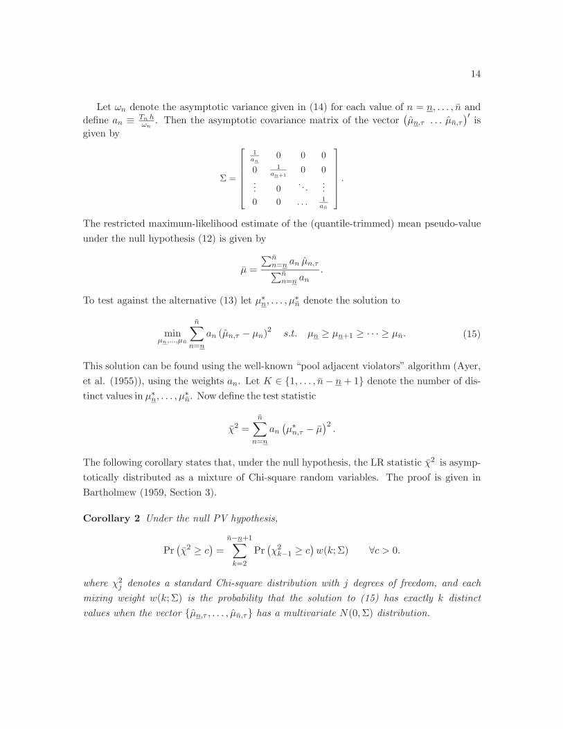
Let denote the asymptotic variance given in (14) for each value of = ¯ and

de ne . Then the asymptotic covariance matrix of the vector¡ˆ ˆ¯

¢0is

given by

=

1 0 0 0

0 1+1

0 0

... 0. . .

...

0 0 1¯

The restricted maximum-likelihood estimate of the (quantile-trimmed) mean pseudo-value

under the null hypothesis (12) is given by

¯ =

P¯= ˆP¯=

To test against the alternative (13) let ¯ denote the solution to

min¯

X=

(ˆ )2 +1 · · · ¯ (15)

This solution can be found using the well-known “pool adjacent violators” algorithm (Ayer,

et al. (1955)), using the weights . Let {1 ¯ + 1} denote the number of dis-tinct values in ¯. Now de ne the test statistic

¯2 =X=

¡¯¢2

The following corollary states that, under the null hypothesis, the LR statistic ¯2 is asymp-

totically distributed as a mixture of Chi-square random variables. The proof is given in

Bartholmew (1959, Section 3).

Corollary 2 Under the null PV hypothesis,

Pr¡¯2

¢=

¯ +1X=2

Pr¡21

¢( ; ) 0

where 2 denotes a standard Chi-square distribution with degrees of freedom, and each

mixing weight ( ; ) is the probability that the solution to (15) has exactly distinct

values when the vector {ˆ ˆ¯ } has a multivariate (0 ) distribution.

15

3.2 A Sup-Norm Test Using Subsampling

A second testing approach is based on a Kolmogorov-Smirnov-type statistic for a -sample

test of equal distributions against an alternative of strict rst-order stochastic dominance.

Consider the sum of supremum distances between successive empirical distributions of

pseudo-values:14

=1X

=

sup[ 1 ]

nˆˆ +1( )

ˆˆ ( )

oUniform consistency of each ˆ

ˆ (·) on the compact set [ 1 ] implies that 0 as

under 0, while 0 under 1. This forms a basis for testing. In

particular, de ne the test statistic

=

where is a normalizing sequence proportional to³

2

log

´1 2, the rate of uniform conver-

gence of each ˆˆ (·) to the corresponding (·) .To approximate the asymptotic distribution of the test statistic, we use a subsampling

approach.15 Recall that the observables consist of the set of bids = ( 1 ) from

each auction = 1 . So we can write

=¡

1

¢Let denote a sequence of subsample sizes. For each , let be a sequence proportional

to Let

=X=

μ ¶denote the number of subsets

³1

´of ( 1 ) consisting of all bids

from of the original -bidder auctions, = . Let denote the statistic³1

´obtained using the th such subsample of bids. The sampling

distribution of the test statistic is then approximated by

( ) =1 X

=1

1 { } (16)

The critical value for a test at level is taken to be the 1 quantile, 1 , of

14Wallenstein (1980) proposed a version of this statistic for testing in the case of iid draws from di erentdistributions. In that special case, the exact sampling distribution can be derived.15See Linton, Massoumi and Whang (2002) for a recent application of subsampling to tests for stochastic

dominance in a di erent context.

16

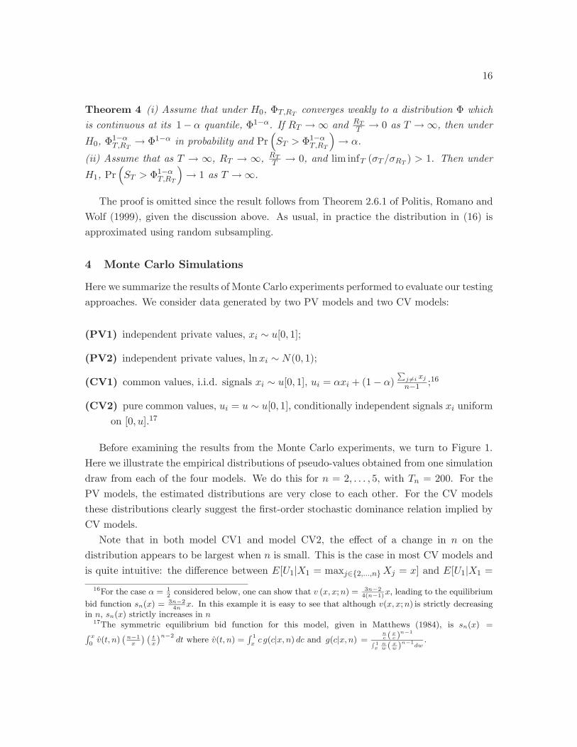
Theorem 4 (i) Assume that under 0, converges weakly to a distribution which

is continuous at its 1 quantile, 1 . If and 0 as , then under

0,1 1 in probability and Pr

³1

´.

(ii) Assume that as , , 0, and lim inf ( ) 1. Then under

1, Pr³

1´

1 as .

The proof is omitted since the result follows from Theorem 2.6.1 of Politis, Romano and

Wolf (1999), given the discussion above. As usual, in practice the distribution in (16) is

approximated using random subsampling.

4 Monte Carlo Simulations

Here we summarize the results of Monte Carlo experiments performed to evaluate our testing

approaches. We consider data generated by two PV models and two CV models:

(PV1) independent private values, [0 1];

(PV2) independent private values, ln (0 1);

(CV1) common values, i.i.d. signals [0 1], = + (1 )P

6=1 ;16

(CV2) pure common values, = [0 1], conditionally independent signals uniform

on [0 ].17

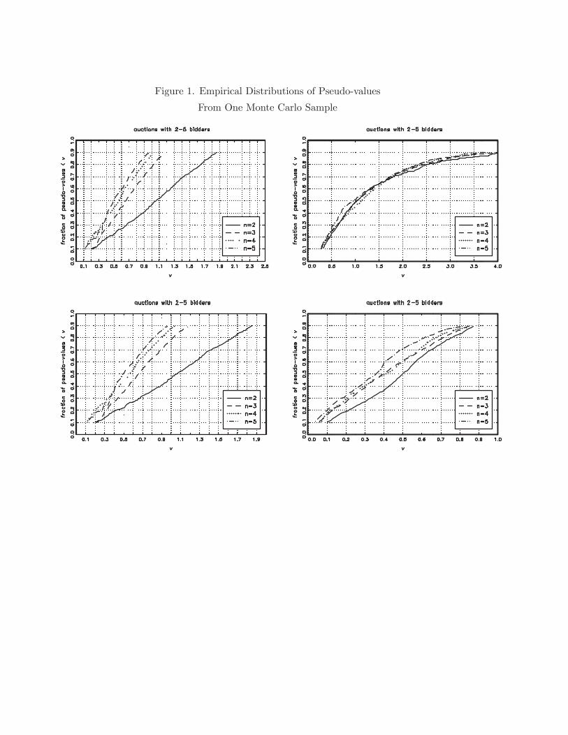
Before examining the results from the Monte Carlo experiments, we turn to Figure 1.

Here we illustrate the empirical distributions of pseudo-values obtained from one simulation

draw from each of the four models. We do this for = 2 5, with = 200. For the

PV models, the estimated distributions are very close to each other. For the CV models

these distributions clearly suggest the rst-order stochastic dominance relation implied by

CV models.

Note that in both model CV1 and model CV2, the e ect of a change in on the

distribution appears to be largest when is small. This is the case in most CV models and

is quite intuitive: the di erence between [ 1| 1 = max {2 } = ] and [ 1| 1 =

16For the case = 12 considered below, one can show that ( ; ) = 3 2

4( 1) , leading to the equilibrium

bid function ( ) = 3 24

. In this example it is easy to see that although ( ; ) is strictly decreasingin , ( ) strictly increases in17The symmetric equilibrium bid function for this model, given in Matthews (1984), is ( ) =R0ˆ( )

¡1¢ ¡ ¢ 2

where ˆ( ) =R 1

( | ) and ( | ) =( ) 1R 1 ( ) 1

17

max {2 +1} = ] typically shrinks as grows. This is important since most auction

data sets contain relatively few observations for large but many observations for small–

exactly where the e ects of the winner’s curse are most pronounced.

We rst consider the LR test, based on quantile-trimmed means. Tables 1 and 2 sum-

marize the test results, using tests with nominal size 5% and 10%. The last two rows in

Table 1 indicate that in the two PV models there is a tendency to over-reject. For example,

for tests with nominal size 10% and data generated by the PV1 model, we reject 20.5% of

the time when the range of bidders is 2—4, and 39% of the time when the range of bidders

is 2—5. The tests do appear to have good power properties, rejecting the CV models in 70

to 100 percent of the replications. However, the over-rejection under the null is a concern.

One possible reason for the over-rejections is that the asymptotic approximations of the

variances of the average pseudo-values ( in Corollary 3) may be poor at the modest sample

sizes we consider. We have considered an alternative of using bootstrap estimates of . The

results, reported in Table 2, indicate that the tendency towards over-rejection is attenuated

when we estimate these variances with the bootstrap. For a test with nominal size 10%,

we now reject no more than 13.5% of the time when the range of is 2—4, and 18% of the

time when the range of is 2—5. With a 5% nominal size, our rejection rates range between

4% and 11.5%. The power properties remain very good. These results are encouraging and

suggest use of the bootstrap in practice.

Finally, Table 3 provides results for the Kolmogorov-Smirnov test using random sub-

sampling to obtain critical values.18 This test appears to perform extremely well. The

rejection rates for the two PV models are very close to the nominal sizes in all cases. The

rejection rates for the CV models are also extremely high, particularly when more than two

distributions are compared.

5 Endogenous Participation

Thus far we have assumed that variation in participation across auctions is exogenous to

the joint distribution of bidders’ valuations and signals. Such exogenous variation could

arise, for example, from exogenous shocks to bidders’ costs of participation, exogenous

variation in bidder populations across markets, or seller restrictions on participation–e.g.,

18Here we have incorporated the recentering approach suggested by Chernozhukov (2002). Ineach subsample, the test statistic was recentered by the original full-sample test statistic: Lq

2

log

hP¯ 1= sup

³ˆ+1( ) ˆ ( )

´Kiwhere

P¯ 1 sup³ˆ+1( ) ˆ ( )

´, the full-sample

statistic. The subsampled -value is computed as 1P

=1 1

μL

q2

logK¶.

18

in government auctions (McAfee and McMillan (1987)) or eld experiments (Engelbrecht-

Wiggans, List, and Lucking-Reiley (1999)). However, in many applications participation

may be endogenous. Here we explore adaptation of our testing approach to such situations,

considering several di erent models of participation.

5.1 Binding Reserve Prices

The most common model of endogenous participation is one in which the seller uses a

binding reserve price , so that only bidders with su ciently favorable signals bid. We

continue to let denote the number of potential bidders and will now let denote the

number of actual bidders–those submitting bids of at least . Variation in the number

of potential bidders is still taken to be exogenous; i.e., Assumption 4 is maintained in this

case. However, will be determined endogenously. Because we consider sealed bid auctions

with private information, it is natural to assume that bidders know the realization of

but not that of when choosing their bids, since is determined by the realizations of the

signals.19 We assume the researcher also can observe .20 As before, we let (·) denotethe distribution of the values ( ) of the potential bidders.

As shown by Milgrom and Weber (1982), given and , a bidder participates if and only

if his signal exceeds the “screening level”

( ) = inf

½: | = max

6=

¸ ¾(17)

That is, a bidder participates only if he would be willing to pay the reserve price for the

good even when no other bidder were. In a PV auction, we may assume without loss of

generality that [ | = ] = . Since in a PV model [ | = max 6= ] =

[ | = ], (17) then implies ( ) = . In a common values model, however,

[ | = max 6= ] decreases in (the proof follows that of Theorem 1), im-

plying that ( ) increases in . This gives the following lemma, which will imply that

our baseline testing approach must be modi ed in this case.

Lemma 1 The screening level ( ) is invariant to in a PV model but strictly increas-

ing in in a CV model.

19Schneyerov (2002) considers a di erent model in which bidders observe a signal of the number of actualbidders after the participation decision but before bids are made.20See HPP for an example. If this is not the case, not only is testing di cult, but the more fundamental

identi cation of bidders’ values ( ) generally fails. This is because bidding is based on a rst-ordercondition for bidders who condition on the realization of when constructing their beliefs ( ; ) regardingthe most competitive opposing bid. Identi cation based on this rst-order condition requires that theresearcher condition on the same information available to bidders.

19

For both PV and CV models, the equilibrium participation rule implies that the marginal

distribution of the signals of actual bidders is the truncated distribution

( | ) =( ) ( ( ))

1 ( ( ))

Hence, letting

( ) = ( ( ) ( ) )

the distribution of values for actual bidders is given by

( ) =( ) ( ( ))

1 ( ( ))( ) (18)

In a PV model, ( | ) = ( ) ( )1 ( ) . Since neither this distribution nor the expectation

( ) varies with in a PV model, it is then still the case that the distribution (·)is invariant to in a PV model, implying that (·) is too. However, the CV case doesnot give a clean prediction about (·). Because ( ) increases with under common

values, changes in a ect the marginal distribution of actual bidders’ values in two ways:

rst by the fact that ( ) decreases in for xed ; second by the fact that as

increases, only higher values of are in the sample. The rst e ect creates a tendency

toward the FOSD relation derived in Theorem 1 for CV models, while the second e ect

works in the opposite direction. This leaves the e ect on ( ) of an exogenous change in

ambiguous in a CV model. However, we can obtain unambiguous predictions under both

the PV and CV hypotheses by exploiting the following result.

Lemma 2 ( ( )) is identi ed.

Proof: Let ˜ (·) denote the joint distribution of signals 1 in an -bidder auction.

Nondegeneracy and exchangeability imply

( ( )) = ( ( )) = ˜ ( ( ) ) (19)

Observe that

Pr( = 0| = ) = ˜ ( ( ) ( ) ( ))

while

Pr (0 | = ) =h˜ ( ( ) ) ˜ ( ( ) ( ) ( ))

iHence, using (19),

( ( )) =Pr (0 | = )

+ Pr( = 0| = ) (20)

20

¤

With ( ( )) known for each , we can then reconstruct ( ) for all ( ).

In particular, from (18) we have

( ) = [1 ( ( ))] ( ) + ( ( )) ( ) (21)

Theorem 5 ( ) is identi ed for all ( ).

Proof: Noting that with a binding reserve price

( | ) = Pr( = 1| = = ) +X=2

Pr( = max{1 2 }\

| = = )

the observables and the rst-order condition (4) uniquely determine ( 1( ) 1( ) ) for

all and ( ( )). This determines the distribution (·). Lemma 2 and (21) thengive the result. ¤Testable implications of the PV and CV models for the distribution ( ) were es-

tablished in Corollary 1, and estimation is easily adapted from that for the baseline case

using sample analogs of the distributions in the identi cation results above. However, note

that we cannot compare the distributions ( ) in their (truncated) left tails, but rather

only on regions of common support of the distributions (·). In particular, since ( )

is nondecreasing in we can perform a test (using the estimation and testing approaches

developed above) of21

0 : ( ) = 3( ) = · · · = ¯( ) ( ¯) (22)

against

1 : ( ) 3( ) · · · ¯( ) ( ¯) (23)

which are implied by (8) and (9), respectively.22 While this provides an approach for con-

sistent testing, the fact that we must restrict the region of comparison could be a limitation

of this approach in nite samples, particularly if the true model is one in which the e ects

21 ( ) is just the lowest value of ( ) for an actual bidder and is therefore easily estimated fromthe pseudovalues.22We have assumed here that is xed across auctions. This is not necessary. Indeed, as GPV have

suggested, variation in can enable one to trace out more of the distribution (·) by extending methodsfrom the statistics literature on random truncation. A full development of this extension, however, is a topicunto itself and not pursued here.

21

of the winner’s curse are most pronounced for bidders with signals in the left tail of the

distribution. However, note that a signi cant di erence between ( ¯) and ( ) for

(the reason a test of (22) vs. (23) would involve a substantially restricted support)

is itself evidence inconsistent with the PV hypothesis but implied by the CV hypothesis.

Hence, a complementary testing approach is available based on the following theorem.

Theorem 6 Under the PV hypothesis, ( ( )) is identical for all . Under the CV

hypothesis, ( ( )) is strictly increasing in .

Proof: Since ( ( )) = ( ( )), the result follows from Lemma 1. ¤

Consistent estimation of ( ( )) for each is easily accomplished with sample

analogs of the probabilities on the right-hand side of (20).23 A multivariate one-sided

hypothesis test similar to those developed above could then be applied.

5.2 Costly Participation

Endogenous participation also arises when it is costly for bidders to participate. In some

applications preparing a bid may be time consuming. In others, learning the signal

might require estimating costs based on detailed contract speci cations, soliciting bids from

subcontractors for a construction project, or analyzing seismic surveys of o shore oil tracts.

Because bidders must recover these costs on average, for large enough it is not an equilib-

rium for all bidders to participate in the auction, even if bidders are certain to place a value

on the good strictly above the reserve price (if any). We consider two standard models of

costly participation from the theoretical literature.

5.2.1 Bid Preparation Costs

Samuelson (1985) studied a model in which bidders rst observe their signals and the reserve

price , then decide whether to incur a cost of preparing a bid. Samuelson considered

only the independent private values model; however, for our purposes this model of costly

participation is equivalent to one in which the seller charges a participation fee (a bidder’s

participation decision and rst-order condition are the same regardless of whether the fee is

paid to the seller, to an outside party, or simply “burned”). The case of a participation fee

paid to the seller has been treated by Milgrom and Weber (1982) for the general a liated

values model.24

23The de nitions of ˆ ( ; ) and ˆ ( ; )would require the obvious modi cations to account for the factthat only bids, not , are observed in each auction with potential bidders.24We will assume that their “regular case” (pp. 1112—1113) obtains.

22

Given and , participation is again determined by the realization of signals and a

screening level

( ) = inf

½:

Z[ ( ) ] ( | )]

¾Unlike the model in the preceding section, here the screening level ( ) varies with

even with private values, since ( | ) varies with . However, a valid testing approach

can nonetheless be developed in a manner nearly identical to that above. In particular, the

argument used to prove Lemma 2 also implies the following result.

Lemma 3 With a reserve price and bid preparation cost , ( ( ( ) ( ) ))

is identi ed from observation of and

Letting ( ) now denote ( ( ) ( ) ), the rst-order condition (4) and

equation (21) can then be used to construct ( ) for all ( ¯), enabling testing

of the hypotheses (22) vs. (23) as in the preceding section.

5.2.2 Signal Acquisition Costs

A somewhat di erent model is considered by Levin and Smith (1994).25 In that model,

each bidder chooses whether to incur cost in order to learn (or to process) his signal

and submit a bid. Bidders know and observe the number of actual bidders before

they bid. Levin and Smith derive a symmetric mixed strategy equilibrium in which each

potential bidder’s participation decision is a binomial randomization. With no reserve price,

this leads to exogenous variation in . Because is observed by bidders prior to bidding

in their model, our analysis for the case of exogenous variation in then carries through

directly, substituting for .26

5.3 Unobserved Heterogeneity

The last model of endogenous participation we consider is the most challenging empiri-

cally. Here participation is determined in part by unobserved factors that also a ect the

distribution of bidders’ valuations and signals. Intuitively, if auctions with large numbers

25Li (2002) has considered parametric estimation of the symmetric IPV model for rst-price auctionsunder this entry model.26If, in addition, there were a binding reserve price, only bidders who paid the signal acquisition cost and

observed su ciently high signals would participate. The mixed strategies determining signal acquisition,however, still result in exogenous variation in the number of “informed bidders,” , a subset of whomwould obtain su ciently high signals to bid. In this case testing would be possible following the approachin the preceding section, but with replacing .

23

of bidders tend to be those in which the good is known by bidders to be of particularly high

(or low) value, tests based on an assumption that variation in participation is exogenous

can give misleading results. In general, unobserved heterogeneity introduces serious chal-

lenges to the nonparametric identi cation of the rst-price auction model that underlies

our approach (recall footnote 20).27 However, in some cases this problem can be overcome

i nstrumental variables are available.

Suppose that the number of actual bidders at each auction is determined by two scalar

factors, and . Bidders observe both, but the researcher observes only . While we will

refer to as the instrument, it may in fact be a function (known or estimated) of a vector

of instruments I. summarizes the e ects of unobservables on participation and may be

correlated with bidders’ valuations. We make the following assumptions:

Assumption 6 is independent of ( 1 ¯ 1 ¯ )

Assumption 7 = ( ), with nondecreasing in and strictly increasing in

Assumption 6 allows the possibility that is correlated with ( 1 ¯ 1 ¯),

but requires that the instrument is not. In Assumption 7, monotonicity of in is the

requirement that the instrument be positively correlated with the endogenous variable .

Weak monotonicity of (·) in the unobservable would be only a normalization. The strict

monotonicity assumed here is a restriction that requires to be discrete. The important

implication is that conditioning on ( ) is then equivalent to conditioning on ( ).28

More precisely, letting ˜ (·) denote the joint distribution of 1 1 , etc.,

˜ ( 1 1 | = ( ) = = = ) =

˜ ( 1 1 | = = )

While might just be the number of potential bidders , it need not be. For example,

one structure consistent with Assumptions 7 and 6 is the model

= (I) +

where = (I) is a function (possibly unknown) of a vector of instruments I, and is

independent of I.

27Krasnokutskaya (2003) has recently shown that methods from the literature on measurement error canbe used to enable estimation of a particular private values model in which unobserved heterogeneity entersmultiplicatively (or additively) and is independent of the idiosyncratic components (themselves indepen-dently distributed) of bidders’ values.28If the relationship between and were only weakly monotone, conditioning on ( ) would be

equivalent to conditioning on ( ) and the event W for some set W. In some applications this maybe su cient to enable the use of the rst-order condition (4) as a useful approximation.

24

The following example illustrates the problem that this type of model can create for our

basic testing approach.

Example. Consider the simple linear model

= + 1

= + 2

= ( )

where (·) is strictly increasing in both and , which are discrete random variables;

the disturbance terms 1 and 2 are mean zero and independent of and ; and2 are independent; but 1 and are correlated. Assuming is not degenerate, one

obtains a PV model if 2 is degenerate and a CV model otherwise. Letting ( ; ) =

[ | max 6= = = ], under the PV hypothesis,

( ( ; ) ) = ( | = )

= ( + 1 | ( ) = )

6= ( + 1 | ( ) = + 1)

where the inequality follows from the correlation of 1 and . Hence, under the PV null the

distribution of ( ; ) varies with . Likewise, under the CV alternative, the stochastic

dominance relation of Corollary 1 need not hold. ¦

To see how this problem can be overcome, rst de ne

( ; ) | = max6=

= ( ) = =

¸(24)

We can consistently estimate each ( ; ) by rst conditioning on and to construct

estimates of

( | ) = Pr(max6=

| = = = )

and the corresponding conditional density ( | ) in order to exploit the rst-order con-

dition (the analog of (4))

( ; ) = +( | )( | ) (25)

As before, this rst-order condition enables recovery of estimates of each ( ; )

25

from the observed bids. Now, observe that

Pr ( ( ; ) ) = Pr ( ( ; ( ) ) )

= Pr

μ1| 1 = max

{2 ( )}= =

¸ ¶= Pr

μ1| 1 = max

{2 ( )}=

¸ ¶where the nal equality follows from Assumption 6.

Assumption 7 and the proof of Theorem 1 imply that the last expression above is strictly

increasing in in a CV auction (for any ) but invariant to in a PV auction. Hence our

testing approaches are still applicable if we rely on exogenous variation in the instrument

rather than exogenous variation in or . In particular, after estimating pseudo-values

using equation (25), one can pool pseudo-values across all values of while holding xed

to then compare the empirical distributions of the pseudo-values across values of . We

emphasize that while the comparison of distributions of pseudo-values forming the test

for common values is done pooling over , the estimation of pseudo-values must be done

conditioning on both and .

6 Observable Heterogeneity

While we assumed above that data were available from auctions of identical goods, in

practice this is rarely the case. In our application below, as in many others, we observe

auction-speci c characteristics that are likely to shift the distribution of bidder valuations.

The results above can be extended to incorporate observables using standard nonparametric

techniques. Let Y be a vector of observables and de ne y( | ) = Pr(max 6= | =

= Y = y) etc. One simply substitutes y( | )y( | ) for

( | )( | ) on the right-hand side of

the rst-order condition (4) and

( y) [ | = max6=

= Y = y]

on the left-hand side. Standard smoothing techniques can be used to estimate y( | )y( | ) .

With many covariates, however, estimation will require large data sets. An alternative

that may be more useful in many applications can be applied if we assume

( y) = ( ) + (y) (26)

withY independent of 1 . This additively separable structure is particularly useful

26

because it is preserved by equilibrium bidding.29

Lemma 4 Suppose that Y is independent of X and (26) holds. Then the equilibrium bid

function, conditional on Y = y, has the additively separable form ( ; y) = ( ; )+ (y).

The proof follows the standard derivation of the equilibrium bid function for a rst-

price auction (only the boundary condition for the di erential equation (1) changes) and

is therefore omitted. An important implication of this result is that we can account for

observable heterogeneity in a two-stage procedure that avoids the need to condition on

(smooth over) Y when estimating distributions and densities of bids. First note that,

letting

0( ) = [ ( ; )]

and

0 = y[ (y)]

we can write the equilibrium bidding strategy as

( ; y) = 0( ) + 0 + 1(y) + 1( ; )

where 1( ; ) has mean zero conditional on ( y). Now observe that

0( ) + 0 + 1( ; ) (27)

is the bid that bidder would have submitted in equilibrium in a generic (i.e., 1(y) = 0)

-bidder auction. Our tests can then be applied using the “homogenized” bids constructed

using estimates of (27).

To implement this approach, in the rst stage we regress all observed bids on the co-

variates Y and a set of dummy variables for each value of . The sum of each residual

and the corresponding intercept estimate provides an estimate of each . In the second

stage, these estimates are treated as bids in a sample of auctions of homogeneous goods.

Note that the function 1(·) is estimated in the rst stage regression using all bids in the

sample rather than separately for each value of . This can make it possible to incorporate

a large set of covariates and can make a exible (or even nonparametric) speci cation of

1(·) feasible.Adapting this approach to the models of endogenous participation discussed above is

straightforward. The case requiring modi cation is that in which instrumental variables are

29If the covariates enter multiplicatively rather than additively, an analogous approach to that proposedbelow can be applied.

27

used. There the intercept of the equilibrium bid functions ( ; y ) will now vary with

both and (or, equivalently, with both and ). Under the assumptions of section 5.3,

one needs only to include separate intercepts 0( ) + 0 (replacing 0( ) + 0 above) for

each combination of and in the rst stage. One then treats the sum of the ( )-speci c

intercept and the residuals from the corresponding auctions as the homogenized bids in the

second stage.

Finally, note that the asymptotic properties of the ultimate test statistic are not a ected

by the rst stage as long as the rst-stage estimates converge at a faster rate than the

pseudo-value estimates, as is guaranteed if the rst stage is parametric.

7 Application to U.S. Forest Service Timber Auctions

7.1 Data and Background

We apply our tests to timber auctions run by the United States Forest Service (USFS). In

each sale, a contract for timber harvesting on federal land was sold by rst-price sealed bid

auction.30 Detailed descriptions of the auctions can be found in Baldwin (1995), Baldwin,

Marshall, and Richard (1997), Athey and Levin (2001), Haile (2001), or Haile and Tamer

(2003). We discuss only a few key features that are particularly relevant to our analysis.

Despite considerable attention to these auctions in the literature, there has been disagree-

ment about whether they should be viewed as common or private value auctions. There

are, in fact, two very di erent types of Forest Service auctions, for which the signi cance of

common value elements may be di erent.

The rst type of auction is known as a lumpsum sale. As the term suggests, here bidders

submit a total bid for the entire volume of timber on the tract. The winning bidder pays his

bid regardless of the volume actually realized at the time of harvest. Bidders, therefore, may

face considerable common uncertainty over the volume of timber on the tract, since this can

only be estimated ex ante. More signi cant, bidders often conduct their own “cruises” of

tract before the auction to form their own estimates. Of course, private cruises may provide

information about common or private value features of the tract. Furthermore, before each

sale, the Forest Service conducts its own cruise of the tract to provide bidders with estimates

of (among other things) timber volumes by species, harvesting costs, costs of manufacturing

end products from the timber, and selling prices of these end products. This creates a great

deal of common knowledge information about the tract. Whether su cient scope remains

30The forest service also conducts English auctions, although we do not consider these here.

28

for private information regarding features common to all bidders is uncertain, although our

a priori belief was that lumpsum sales were likely possess common value elements.

The second type of auction is known as a “scaled sale.” Here, bids are made on a per

unit (thousand board-feet of timber) basis, with the winner selected based on these unit

prices ex ante estimates of timber volumes. However, actual payments to the Forest Ser-

vice are based on actual volumes, measured by a third party at the time of harvest. As a

result, the importance of common uncertainty regarding tract values may be reduced. In

fact, bidders are less likely to send their own cruisers to assess the tract value (National

Resources Management Corporation (1997)). This may leave less scope for private informa-

tion regarding any shared determinants of bidders’ valuations and, therefore, less scope for

common values. Bidders may, however, have private information of an idiosyncratic (PV)

nature regarding their own sales and inventories of end products, contracts for future sales,

or inventories of uncut timber from private timber sales. This has led several authors (e.g.,

Baldwin, Marshall, and Richard (1997), Haile (2001), Haile and Tamer (2003)) to assume a

private values model for scaled sales.31 However, this is not without controversy; Baldwin

(1995) and Athey and Levin (2001) argue for a common values model even for scaled sales.32

We will separately consider lumpsum sales and scaled sales. With our formal tests, we

hope to evaluate both the question of whether common value elements are present in these

auctions, and the question of whether a priori intuition regarding this question is reliable.

The auctions in our samples took place between 1982 and 1990 in Forest Service regions

1 and 5. Region 1 covers Montana, eastern Washington, Northern Idaho, North Dakota,

and northwestern South Dakota. The Region 5 data consist of sales in California. The

restriction to sales after 1981 is made due to policy changes in 1981 that (among other

things) reduced the signi cance of subcontracting as a factor a ecting bidder valuations,

since resale opportunities can alter bidding in ways that confound the empirical implications

of the winner’s curse (cf. Haile (2001), Bikhchandani and Huang (1989), and Haile (1999)).

For the same reason, we restrict attention to sales with no more than 12 months between

the auction and the harvest deadline.33 For consistency, we consider only sales in which the

Forest Service provided ex ante estimates of the tract values using the predominant method

31Other studies assuming private values at timber auctions (USFS and others) include Cummins (1994),Elyakime, La ont, Loisel, and Vuong (1994), Hansen (1985), Hansen (1986), Johnson (1979), Paarsch (1991),and Paarsch (1997).32Other studies assuming common values models for Forest Service timber auctions include Chatterjee

and Harrison (1988), Lederer (1994), and Le er, Rucker, and Munn (1994).33This is the same rule used by Haile and Tamer (2003) and the opposite of that used by Haile (2001) to

focus on sales with signi cant resale opportunities.

29

of this time period, known as the “residual value method.”34 We also exclude salvage sales,

sales set aside for small rms, and sales of contracts requiring the winner to construct roads.

Table 4 describes the resulting sample sizes for auctions with each number of bidders

= 2 3 12. There are fairly few auctions with more than 4 bidders, particularly in

the sample of lumpsum sales. However, the unit of observation, both for estimation of the

pseudo-values and estimation of the distribution of pseudo-values, is a bid. Our data set

contains 75 or more bids for auctions of up to seven bidders in both samples.

Our data set includes all bids35 for each auction, as well as a large number of auction-

speci c observables. These include the year of the sale, the appraised value of the tract,

the acreage of the tract, the length (in months) of the contract term, the volume of timber

sold by the USFS in the same region over the previous six months, and USFS estimates of

the volume of timber on the tract, harvesting costs, costs of manufacturing end products,

selling value of the end products, and an index of the concentration of the timber volume

across species.36 All dollar values are in constant 1983 dollars per thousand board-feet of

timber. Table 5 provides summary statistics.

7.2 Results

We rst perform the tests on each sample under the assumption of exogenous participation.

We consider comparisons of auctions with up to 7 bidders, although we look at ranges

of 2—3, 2—4, 2—5, and 2—6 bidders as well. We use the method described in section 6 to

eliminate the e ects of observable heterogeneity with a rst-stage regression of bids on the

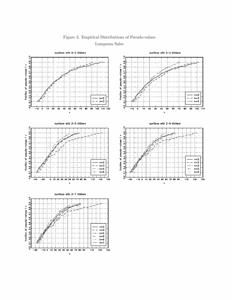
covariates listed above. Figures 2 and 3 show the estimated distributions of pseudo-values

for each of these comparisons. The distributions compared appear to be roughly similar,

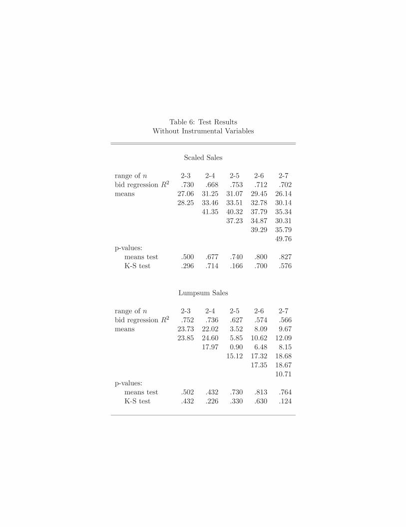
although there is certainly some variation. Table 6 reports the formal test results. For each

speci cation we report the 2 from the rst-stage regression of bids on auction covariates,

the means of each estimated distribution of pseudovalues, and the p-value associated with

each test of the private values null hypothesis. The t of the rst-stage bid regressions

are generally very good (recall that bids are already normalized by the size of the tract).

Both the means test and the K-S test fail to reject the null hypothesis of private values at

34See Baldwin, Marshall, and Richard (1997) for details.35In practice separate prices are bid for each identi ed species on the tract. Following, e.g., Baldwin,

Marshall, and Richard (1997), Haile (2001), and Haile and Tamer (2003), we consider only the total bid ofeach bidder, which is also the statistic used to determine the auction winner. See Athey and Levin (2001)for an analysis of the distribution of bids across species.36This concentration index is equal to the sum of the squared shares of each species on the tract. Because

sawmills typically are highly specialized, a tract consisting primarily of a single species may be more valuablethan another with the same volume spread over many species.

30

standard levels in any speci cation.

One possible reason for a failure to reject the null is the presence of unobserved het-

erogeneity correlated with the number of bidders.37 If tracts of higher value in unobserved

dimensions also attracted more bidders, for example, there would be a tendency for the

distributions compared to shift in the direction opposite that predicted by the winner’s

curse, and there is some suggestion of this in the graphs. Hence, we also perform the

test using the model of endogenous participation with unobserved heterogeneity discussed

in section 5.3.38 As instruments, I, we use the numbers of sawmills and logging rms in

the county of each sale or neighboring counties (cf. Haile (2001)). This approach adds a

second least-squares projection to construct = (I) = [ |I]. For the comparison ofpseudo-value distributions, we split the sample into thirds (halves when we compare only

2- and 3-bidder auctions) based on the number of predicted bidders. Figures 4 and 5 show

the resulting empirical distributions of pseudo-values compared in each test. For the scaled

sales, the distributions are generally close and exhibit no clear ordering. For the lumpsum

sales the distributions also appear to be fairly similar, although most comparisons suggest

the stochastic ordering predicted by a CV model. The formal testing results are given in

Table 7. THe means tests again fail to reject the PV model in any speci cation. In one of

the scaled sale speci cations ( = 2 4) the K-S test would reject at the 10 percent level

(p-value .088). In two of the lumpsum sale speci cations ( = 2 4 2 7) the K-S

test would reject at the 10 percent level or better (p-values of .048 and .080).

As a speci cation check, we have examined the relationship between the estimated

pseudo-values and the associated bids. Under the maintained assumptions of equilibrium

bidding in the Milgrom-Weber model, this relation must be strictly monotone. While test-

ing this restriction has been suggested by GPV and LPV, we are not aware of any formal

testing approach that is directly applicable (cf. GPV). However, here this does not appear

to be essential in our case; the importance of a formal test is in giving the appropriate

allowance for deviations from strict monotonicity that would arise from sampling error. In

most cases we have no deviations from strict monotonicity, so that no formal test could

reject. In particular, we have examined the relation between bids and estimated pseudoval-

ues in each subset of the data used to estimate the pseudovalues. For the case in which no

instrumental variables are used (so that the samples are divided based on the value of ) we

37Haile (2001) provides some evidence using a di erent set of USFS auactions.38We continue to assume the absence of a binding reserve price. See, e.g., Mead, Schniepp, and Watson

(1981), Baldwin, Marshall, and Richard (1997), Haile (2001), Haile and Tamer (2003) for arguments thatForest Service reserve prices are nonbinding, explanations for why this might be the case, and supportingevidence.

31

nd violations only in the case of lumpsum sales with = 6, and even here only in the right

tail. When instrumental variables are used, the sample is split based on the value of both

and the instrument, leading to smaller samples and greater sampling error. Nonetheless,

even here there are only a few violations. For scaled sales, violations occur at no more than

2 points (i.e., 2 bids) per subsample, and the magnitudes of the violations are extremely

small–on the order of 0.03 to 0.3 percent of the pseudovalues themselves. The handful

of noticeable violations for lumpsum sales again occur only when auctions with = 6 are

examined.

While the failure to nd evidence of common values in the scaled sales is consistent with

a priori arguments for private values o ered in the literature, the very limited evidence

against the PV hypothesis for the lumpsum sales may be more surprising. Of course, the

estimates published following the Forest Service cruise may be su ciently precise that they

leave little role for private information of a common value nature.39 In fact, the cruises

performed by the Forest Service for lumpsum sales are more thorough than those for scaled

sales, a fact re ected in the name “tree measurement sale” given to such sales by the Forest

Service. Hence, the intuitive argument for common values at the lumpsum sales might

simply be misleading. It is, of course, a desire to avoid relying on intuition alone that led

us to pursue a formal testing approach in the rst place.

Nonetheless, we interpret the results with some caution. While we have allowed a rich

class of models in our underlying framework, we have maintained the assumption of equi-

librium competitive bidding in a static game, ruling out collusion and dynamic factors that

might in uence bidding decisions. While an examination of the monotonicity restriction

these assumptions imply provides some comfort, a test of monotonicity cannot detect all

violations of these assumptions. Even if these assumptions are satis ed, our economet-

ric techniques for dealing with endogenous participation and auction heterogeneity have

required additional assumptions and nite sample approximations that may cloud the anal-

ysis. Finally, while our tests are consistent, it could well be that the e ect of the winner’s

curse in these auctions is su ciently small that it is very di cult to detect with the moder-

ate sample sizes available–an interpretation given some support by a graphical comparison

of the estimated distributions. While this this would not rule out the presence of a common

value element altogether, it would suggest that any CV elements are small relative to other

sources of variation in the data.

39The fact that bidders conduct their own tract cruises does not contradict this, since the informationobtained from such cruises could relate primarily to rm-speci c (private value) factors.

32

8 Conclusion and Extensions

We have developed nonparametric tests for common values in rst-price sealed-bid auctions.

The tests are nonparametric, require observation only of bids, and are consistent against

all common values alternatives within Milgrom and Weber’s (1982) general framework.

The tests perform well in Monte Carlo simulations and and can be adapted to incorporate

auction-speci c covariates and a range of models of endogenous participation. In addition to

providing an approach for formal testing, comparing distributions of pseudo-values obtained

from auctions with di erent numbers of bidders provides one natural way for quantifying

the magnitude of any deviation from a private values model. An application to USFS timber

auctions nds almost no signi cant evidence of common values, even for auctions in which

a priori arguments might sugggest a CV model. Limitations of our tests are their reliance

on a maintained assumption of equilibrium bidding, and the absence of dynamics in our

underlying framework.

One further limitation of the approach as we have described it above is an assumption

of symmetry. This is not necessary, however. It is possible to extend our methods to

detect common value elements with asymmetric bidders (i.e., dropping the exchangeability

assumption), as long as at least one bidder participates in auctions with di erent numbers

of competitors. Two modi cations of the basic approach above are required. The rst

is that we must focus on one bidder at a time rather than treating them symmetrically.

In particular, consider, without loss of generality, bidder 1. A test for the presence of

common values for bidder 1 can be based on (e.g.) the pseudo-value corresponding to 1 ,

the empirical -th quantile of the bids submitted by bidder 1 in -bidder auctions:

ˆ 1

Ã1 +

ˆ1 ( 1 )

ˆ1 ( 1 )

!

where ˆ1 ( ) and ˆ1 ( ) are nonparametric estimates analogous to those in equation (5)

above, considering only the bids of bidder 1’s opponents.

Under the PV hypothesis, the population analog, 1, is constant across for all

(0 1). Under the CV alternative, in order to obtain the stochastic ordering40

2 1 3 1 · · · ¯ 1

Here we require the second modi cation: in considering auctions with = 2 3 , we

construct a sequence of sets of opponents faces by bidder 1, e.g., {bidder 2}, {bidder 2,40We use a comparison of quantiles only for illustration. In practice, comparisons of means or of distribu-

tion functions are possible here as above.

33

bidder 3}, {bidder 2, bidder 3, bidder 4}, etc. This structure ensures that the severityof the winner’s curse faced by bidder 1 is unambiguously greater in auctions with larger

numbers of participants, even though opponents are not perfect substitutes for each other.

While constructing such a sequence for large would typically require a great deal of data,

doing so for {2 3} (where the change in the severity of the winner’s curse is typicallylargest) may be feasible in some applications.

Appendix

A Proof of Theorem 2

1. This is a standard result on the -convergence of sample to population quantiles (cf. van derVaart (1999), Corollary 21.5).

2. For simplicity we introduce the notation ( ; ), ( ; ), ˆ ˆ ( ; ) =1P

=1

P=1 1 ( )

¡ ¢and ˆ ˆ ( ; ) = 1

2

P=1

P=1

¡ ¢ ³ ´.

Then we can use a standard rst-order Taylor expansion to write

ˆ¡

1 ( ) 1 ( )¢ ¡

1 ( ) 1 ( )¢=ˆ

ˆ

=ˆ

2(ˆ ) +

³ˆ

´+ (ˆ )

=ˆ ˆ

+ˆ

2(ˆ ˆ )

2( ˆ ) +

³ˆ

´+ (ˆ )

Standard bias calculation for kernel estimation shows that by Assumption 5, both

| ˆ | |Z( ( ; + ) ( ; )) ( ) |

Z| | ( ) =

μ1

2

¶and

| ˆ |¯ Z Z

( ( + ; + ) ( ; )) ( ) ( )

¯=

μ1

2

¶Next it will be shown thatp

2 (ˆ ˆ )

μ01μZ Z

2 ( ) 2 ( )

¶( ; )

¶For this purpose it su ces to show that

lim³p

2 (ˆ ( ; ) ˆ ( ; ))´=1μZ Z

2 ( ) 2 ( )

¶( ; )

34

This is veri ed by the following calculation:Ã12 ·

X=1

X=1

μ ¶ μ ¶¸!

=

Ã12 2

ÃX=1

μ ¶ μ ¶¸!!

=12

½ μ ¶ μ ¶¸+ ( 1)

μ ¶ μ ¶ μ ¶ μ ¶¸6=

¾It is a standard result that μ μ ¶ μ ¶¶

=¡2¢

and it can be veri ed thatμ ¶ μ ¶ μ ¶ μ ¶¸=

¡4¢

Therefore we can write³p2 (ˆ ( ; ) ˆ ( ; ))

´=

12

2

μ ¶2

μ ¶¸+

¡4¢

=1Z Z

12

2

μ ¶2

μ ¶( ) +

¡4¢

=1μZ Z

2 ( ) 2 ( )

¶( ; ) + (1)

where the last equality uses the substitutions = ( )Á and = ( )Á . Finally thesame type of variance calculation shows that³p

2³ˆ ˆ

´´0

Hence the proof for part 2 is complete.

3. Since the sample quantiles of the bid distribution converge at rate to the population quan-tile, which is faster than the convergence rate for the pseudo-values, for large the samplingerror in the th quantile of the bid distribution does not a ect the large sample properties ofthe estimated quantiles of the pseudo-value distribution. For each { 1 }:³

ˆ³

1³ˆ

´1³ˆ

´ ´ˆ ( )

´=

μ1¶=

μ12

¶(28)

A formal proof would proceed using uniform convergence of the kernel estimates of ( ; )and ( ; ) and their derivatives, and stochastic equicontinuity arguments (see for example

35

Andrews (1994) and Pollard (1984)). We omit these rather tedious technical details andproceed by noting that (28) implies that the limiting distribution ofp

2³ˆ³ˆ ;

´ ¡1 ( ) 1 ( )

¢´= { 1 }

is the same as the limiting distribution of the vector

2³ˆ( ( ) ; ) ( )

´= { 1 }

In part 2 we showed that each element of this vector is asymptotically normal with limitvariance given by the diagonal element of . It remains to show that the o -diagonal elementsof are 0. For this purpose it su ces to show, using the standard result that nonparametrickernel estimates at two distinct points (here, two quantiles ( ) and 0 ( 0)) areasymptotically independent; i.e.,

lim³p

2³ˆ( ; ) ( )

´ p2³ˆ( 0 ; ) ( 0 0 )

´´= 0

Using the bias calculation and convergence rates derived in part 2, it su ces for this purposeto show that

lim³p

2 (ˆ ( ; ) ( ; ))p

2 (ˆ ( 0 ; 0) ( 0 ; 0))´= 0

To show this, rst observe that the left-hand side can be written"12

X=1

X=1

μ ¶ μ ¶12

X=1

X=1

μ0¶ μ

0¶#

=12 2

"X=1

μ ¶ μ ¶ X=1

μ0¶ μ

0¶#

Using the fact that for each , μ ¶ μ ¶¸=

¡2¢

and for each 6= ,μ ¶ μ ¶ μ0¶ μ

0¶¸

=¡4¢

we can further rewrite the covariance function as

12 2

X=1

X=1

μ ¶ μ ¶ μ0¶ μ

0¶¸+

¡2¢

=12 2

X=1

μ ¶ μ ¶ μ0¶ μ

0¶¸+

¡2¢

=1Z Z

( ) ( )

μ+

0¶ μ

+0¶

( + + ) +¡2¢

0

36

B Proof of Theorem 3

Assumption 5 directly implies the following uniform rates of convergence for ˆ ( ; ) and ˆ ( ; )(see Horowitz (1998) and Guerre, Perrigne, and Vuong (2000)).

supR

¯˜ ( ; )

¯supR

¯ˆ ( ; ) ( ; )

¯=

Ãrlog

!+

¡ ¢sup

¯˜ ( ; )

¯sup

¯ˆ ( ; ) ( ; )

¯=

Ãrlog

2

!+

¡ ¢Since part (i) is an immediate consequence of part (ii), we proceed to prove part (ii) directly.

Letting ( ; ) =¡

1 ( ) 1 ( )¢, we can decompose the left hand side of part (ii) asp

(ˆ [ ( ; ) 1 ( 1 )])

=p Ã

1 X=1

X=1

Ã+ˆ ( ; )

ˆ ( ; )

!1³ˆ ˆ

1

´[ ( ; ) 1 ( 1 ])

!=ˆ1 + ˆ2 + ˆ3 + ˆ4

where

ˆ1 =p Ã

1 X=1

X=1

È ( ; )

ˆ ( ; )

( ; )

( ; )

!³1³ˆ ˆ

1

´1 ( 1 )

´!

ˆ2 =p 1 X

=1

X=1

"ˆ ( ; )

ˆ ( ; )

( ; )

( ; )

#1 ( 1 )

ˆ3 =p 1 X

=1

X=1

μ+

( ; )

( ; )

¶³1³ˆ ˆ

1

´1 ( 1 )

´=p 1 X

=1

X=1

( ; )³1³ˆ ˆ

1

´1 ( 1 )

´ˆ4 =

p 1 X=1

X=1

μμ+

( ; )

( ; )

¶1 ( 1 ) [ ( ; ) 1 ( 1 )]

¶

=p 1 X

=1

X=1

( ( ; ) 1 ( 1 ) [ ( ; ) 1 ( 1 )])

We consider the properties of each of these terms in turn. For ˆ4 , a standard application of thelaw of large numbers gives

ˆ4 = (1) = (1)

The function in the summand of ˆ3 satis es stochastic equicontinuity conditions (a type I function

of Andrews (1994)). Hence using the parametric convergence rates of ˆ and ˆ1 ,

ˆ3 =p ³

( ; ) 1³ˆ ˆ

1

´[ ( ; ) 1 ( 1 )]

´+ (1)

=p ³ ³

ˆ´+

³ˆ1 1

´´+ (1) =

p μ1¶+ (1) = (1)

37

Similarly, the function in the summand of ˆ1 also satis es stochastic equicontinuity conditions(product of type I and type III functions in Andrews (1994)), and hence

ˆ1 =p Ã

ˆ ( ; )

ˆ ( ; )

( ; )

( ; )

!³1³ˆ ˆ

1

´1 ( 1 )

´+ (1)

=

Ãsup

[ 1 + ]

¯ˆ ( ; )

ˆ ( ; )

( ; )

( ; )

¯!p ³ ³ˆ

´+

³ˆ1 1

´´+ (1)

= (1)p μ

1¶+ (1) = (1)

Combining the above results of rates of convergence, we have thus far shown thatp(ˆ [ ( ; ) 1 ( 1 )]) = ˆ2 + (1)

The term ˆ2 can be further decomposed using a second order Taylor expansion:

ˆ2 = ˆ5 + ˆ6 + ˆ7

where

ˆ5 =p 1 X

=1

X=1

1

( ; )

³ˆ ( ; ) ( ; )

´1 ( 1 )

ˆ6 =p 1 X

=1

X=1

( ; )

( ; )2(ˆ ( ; ) ( ; )) 1 ( 1 )

ˆ7 =p 1 X

=1

X=1

1 ( )³ˆ ( ; ) ( ; )

´21 ( 1 )

+p 1 X

=1

X=1

2 ( ) (ˆ ( ; ) ( ; ))21 ( 1 )

Here 1 (·) and 2 (·) are the second derivatives with respect to (·) and (·) evaluated at somemean values between ˆ (·) and (·) and between ˆ (·) and (·). We rst bound ˆ7 using the

uniform convergence rates of ˆ (·) and ˆ (·):¯7

¯ p μ μlog

+ 2

¶+

μlog

2+ 2

¶¶=

μlog

+log

3+p

1+4

¶= (1)

38

Now consider

ˆ6 =p 1 X

=1

X=1

( ; )

( ; )2(ˆ ( ; ) [ˆ ( ; )) 1 ( 1 )]

p 1 X=1

X=1

( ; )

( ; )2 ( [ˆ ( ; )] ( ; )) 1 ( 1 )

=p 1 X

=1

X=1

( ; )

( ; )2 (ˆ ( ; ) [ˆ ( ; )) 1 ( 1 )] + (1)

ˆ8 + (1)

because by assumption the bias in the second term on the right-hand side of the rst line is of theorder p ¡ ¢

=³p

1+2´= (1)

Next we show that

ˆ8

Ã0 =

"Z μZ( ) ( + )

¶2 #"1Z 1(1 )

1( )

( ; )2

( ; )3( )2

#!

This follows from a limit variance calculation for -statistics. We can write

ˆ8 =p 1

2 2

X=1

X=1

( )

where

( ) =X=1

X=1

( ; )2 ( ; )

12

μ ¶ μ ¶12

μ ¶ μ ¶¸1 ( 1 )

Using lemma 8.4 of Newey and McFadden (1994), we can verify thatp | ( ) |=

μp 1¶=

μ1

¶= (1) and

p q( )2

=

μp 13

¶=

μ1

2

¶= (1)

It then follows from Lemma 8.4 of Newey and McFadden (1994) that

ˆ8 =p 1

2

X=1

[ ( ( ) | ) + ( ( ) | )] + (1)

39

The rst term is asymptotically negligible, since

p 12

X=1

( ( ) | )

=p 1 X

=1

£( ; ) 1 ( 1 ) [ ( ; ) 1 ( 1 )] +

¡ ¢¤=p μ

1¶+

³p1+2

´= (1)

It remains only to verify by straightforward though somewhat tedious calculation thatÃp 12

X=1

( ( ) | )

!

=1X

=1

Z1 ( ; )

2 ( ; )

12

μ ¶ μ ¶( )

=1

ÃZ1 ( ; )

2 ( ; )

12

μ ¶ μ ¶( )

!+ (1)

=1

ÃZ1 ( ; )

2 ( ; )

12

μ ¶ μ ¶( )

!2+ (1)"Z μZ

( ) ( + )

¶2 #"1Z 1(1 )

1( )

2 ( ; )3 ( ; )

2 ( )

#

Finally, we note that if we apply the calculations performed for ˆ6 to ˆ5 , we see that£ˆ5

¤= (1) and

¡ˆ5

¢= (1)

which then implies that ˆ5 0. The proof is now completed by putting these terms together.¤

References

Anderson, G. (1996): “Nonparametric Tests of Stochastic Dominance in Income Distri-butions,” Econometrica, 64, 1183—1194.

Andrews, D. (1994): “Empirical Process Methods in Econometrics,” in Handbook ofEconometrics, Vol. 4, ed. by R. Engle, and D. McFadden. North Holland.

(1998): “Hypothesis Testing With a Restricted Parameter Space,” Journal ofEconometrics, 86, 155—199.

Athey, S., and P. Haile (2002): “Identi cation of Standard Auction Models,” Econo-metrica, 70, 2107—2140.

Athey, S., and J. Levin (2001): “Information and Competition in U.S. Forest ServeTimber Auctions,” Journal of Political Economy.

Ayer, M., D. Brunk, G. Ewing, W. Reid, and E. Silverman (1955): “An EmpiricalDistribution Function for Sampling with Incomplete Information,” Annals of Mathemat-ical Statistics, 26, 641—647.

Bajari, P., and A. Hortacsu (2003): “Winner’s Curse, Reserve Prices, and EndogenousEntry: Empirical Insights from eBay Auctions,” RAND Journal of Economics, 34, 329—355.

Baldwin, L. (1995): “Risk Aversion in Forest Service Timber Auctions,” working paper,RAND Corporation.

Baldwin, L., R. Marshall, and J.-F. Richard (1997): “Bidder Collusion at ForestService Timber Sales,” Journal of Political Economy, 105, 657—699.

Barrett, G., and S. Donald (2003): “Consistent Tests for Stochastic Dominance,”Econometrica, 71, 71—104.

Bartholomew, D. (1959): “A Test of Homogeneity for Ordered Alternatives,”Biometrika, 46, 36—48.

Bikhchandani, S., P. Haile, and J. Riley (2002): “Symmetric Separating Equilibriain English Auctions,” Games and Economic Behavior, 38, 19—27.

Bikhchandani, S., and C. Huang (1989): “Auctions with Resale Markets: An Ex-ploratory Model of Treasury Bill Markets,” Review of Financial Studies, 2, 311—339.

Chatterjee, K., and T. Harrison (1988): “The Value of Information in CompetitiveBidding,” European Journal of Operational Research, 36, 322—333.

Chen, X., and X. Shen (1998): “Sieve Extremum Estimates for Weakly Dependent Data,”Econometrica, 66, 289—314.

Chernozhukov, V. (2002): “Inference on Quantile Regression Process, An Alternative,”mimeo., MIT.

Cummins, J. (1994): “Investment Under Uncertainty: Estimates from Panel Data onPaci c Northwest Forest Products Firms,” working paper, Columbia University.

Davidson, R., and J.-Y. Duclos (2000): “Statistical Inference for Stochastic Dominanceand for the Measurement of Poverty and Inequality,” Econometrica, 68, 1435—1464.

Elyakime, B., J. Laffont, P. Loisel, and Q. Vuong (1994): “First-Price Sealed-BidAuctions with Secret Reserve Prices,” Annales d’Economie et Statistiques, 34, 115—141.

Engelbrecht-Wiggans, R., J. List, and D. Lucking-Reiley (1999): “Demand Re-duction in Multi-unit Auctions with Varying Numbers of Bidders: Theory and FieldExperiments,” working paper, Vanderbilt University.

Gilley, O., and G. Karels (1981): “The Competitive E ect in Bonus Bidding: NewEvidence,” Bell Journal of Economics, 12, 637—648.

Guerre, E., I. Perrigne, and Q. Vuong (2000): “Optimal Nonparametric Estimationof First-Price Auctions,” Econometrica, 68, 525—74.

Haile, P. (1999): “Auctions with Resale,” mimeo, University of Wisconsin-Madison.

(2001): “Auctions with Resale Markets: An Application to U.S. Forest ServiceTimber Sales,” American Economic Review, pp. 399—427.

Haile, P., and E. Tamer (2003): “Inference with an Incomplete Model of English Auc-tions,” Journal of Political Economy, 111, 1—51.

Hajek, J., Z. Sidak, and P. Sen (1999): Theory of Rank Tests. Academic Press.

Hansen, R. (1985): “Empirical Testing of Auction Theory,” American Economic Review,Papers and Proceedings, 75, 156—159.

(1986): “Sealed-Bid Versus Open Auctions: The Evidence,” Economic Inquiry,24, 125—143.

Hendricks, K., J. Pinkse, and R. Porter (2003): “Empirical Implications of Equilib-rium Bidding in First-Price, Symmetric, Common-Value Auctions,” Review of EconomicStudies, 70, 115—146.

Hendricks, K., and R. Porter (1988): “An Empirical Study of an Auction with Asym-metric Information,” American Economic Review, pp. 865—883.

Horowitz, J. (1998): “Bootstrap Methods for Median Regression Models,” Econometrica,66, 1327—1352.

Jofre-Bonet, M., and M. Pesendorfer (forthcoming): “Bidding Behavior in a Re-peated Procurement Auction,” Econometrica.

Johnson, R. (1979): “Oral Auction Versus Sealed Bids: An Empirical Investigation,”Natural Resources Journal, 19, 315—335.

Klemperer, P. (1999): “Auction Theory: A Guide to the Literature,” Journal of Eco-nomic Surveys, 13, 227—286.

Krasnokutskaya, E. (2003): “Identi cation and Estimation of Auction Models underUnobserved Auction Heterogeneity,” working paper, Yale University.

Krishna, V. (2002): Auction Theory. Academic Press.

Laffont, J. J., and Q. Vuong (1993): “Structural Econometric Analysis of DescendingAuctions,” European Economic Review, 37, 329—341.

(1996): “Structural Analysis of Auction Data,” American Economic Review, Pa-pers and Proceedings, 86, 414—420.

Lavergne, P., and Q. Vuong (1996): “Nonparametric Selection of Regressors: theNonnested Case,” Econometrica, pp. 207—219.

Lederer, P. (1994): “Predicting the Winner’s Curse,” Decision Sciences, 25, 79—101.

Leffler, K., R. Rucker, and I. Munn (1994): “Transaction Costs and the Collection ofInformation: Presale Measurement on Private Timber Sales,” working paper, Universityof Washington.

Levin, D., and J. Smith (1994): “Equilbrium in Auctions with Entry,” American Eco-nomic Review, 84, 585—599.

Lewbel, A. (1998): “Semiparametric Latent Variable Model Estimation with Endogenousor Mismeasured Regressors,” Econometrica, 66, 105—122.

Li, T. (2002): “Econometrics of First Price Auctions with Entry and Binding ReservationPrices,” working paper, Indiana University.

Li, T., I. Perrigne, and Q. Vuong (2000): “Conditionally Independent Private Infor-mation in OCS Wildcat Auctions,” Journal of Econometrics, 98, 129—161.

(2002): “Structural Estimation of the A liated Private Value Auction Model,”RAND Journal of Economics, 33, 171—193.

Linton, O., E. Massoumi, and Y. Whang (2002): “Consistent Testing for StochasticDominance: A Subsampling Approach,” mimeo., LSE.

McAfee, P., and J. McMillan (1987): Incentives in Government Contracting. Univer-sity of Toronto Press.

McFadden, D. (1989): “Testing for Stochastic Dominance,” in Studies in the Economicsof Uncertainty, ed. by T. B. Fomby, and T. K. Seo. Springer-Verlag.

Mead, W., M. Schniepp, and R. Watson (1981): “The E ectiveness of Competition andAppraisals in the Auction Markets for National Forest Timber in the Paci c Northwest,”Washington: U.S. Department of Agriculture, Forest Service.

Milgrom, P. (1981): “Good News and Bad News: Representation Theorems and Appli-cations,” The Bell Journal of Economics, 13, 380—391.

Milgrom, P., and R. Weber (1982): “A Theory of Auctions and Competitive Bidding,”Econometrica, 50, 1089—1122.

National Resources Management Corporation (1997): “A Nationwide Study Com-paring Tree Measurement and Scaled Sale Methods for Selling United States Forest Ser-vice Timber,” Report to the U.S. Forest Service, Department of Agriculture.

Newey, W. (1994): “Kernel Estimation of Partial Means and a General Variance Estima-tor,” Econometric Theory, 10, 233—253.

Newey, W., and D. McFadden (1994): “Large Sample Estimation and Hypothesis Test-ing,” in Handbook of Econometrics, Vol. 4, ed. by R. Engle, and D. McFadden. NorthHolland.

Paarsch, H. (1991): “Empirical Models of Auctions and an Application to BritishColumbian Timber,” University of Western Ontario, Department of Economics TechnicalReport 91-19.

(1992): “Deciding Between the Common and Private Value Paradigms in EmpiricalModels of Auctions,” Journal of Econometrics, 51, 191—215.

(1997): “Deriving an Estimate of the Optimal Reserve Price: An Application toBritish Columbian Timber Sales,” Journal of Econometrics, 78, 333—357.

Pinkse, J., and G. Tan (2002): “The A liation E ect in First-Price Auctions,” mimeo,Penn State University.

Pollard, D. (1984): Convergence of Stochastic Processes. Springer Verlag.

Samuelson, W. F. (1985): “Competitive Bidding with Entry Costs,” Economics Letters,17, 53—57.

Sareen, S. (1999): “Posterior Odds Comparison of a Symmetric Low-Price, Sealed-BidAuction Within the Common Value and the Independent Private Value Paradigms,”Journal of Applied Econometrics, 14, 651—676.

Schneyerov, A. (2002): “Applying Auction Theory to Municipal Bond Auctions: MarketPower and the Winner’s Curse,” mimeo., University of British Columbia.

van der Vaart, A. (1999): Asymptotic Statistics. Cambridge University Press.

Wolak, F. (1989): “Testing Inequality Constraints in Linear Econometric Models,” Jour-nal of Econometrics, 41, 205—235.

(1991): “The Local Nature of Hypothesis Tests Involving Inequality Constraintsin Nonlinear Models,” Econometrica, 59, 981—995.

Table 1: Monte Carlo Results200 replications of each experiment.

PV1 CV1 PV2 CV2

Range of : 2—4 2—5 2—4 2—5 2—4 3—5 3—5 3—6200 200 200 200 200 200 200 200

share of p-values 10% 0.21 0.39 1.00 1.00 0.12 0.27 0.94 0.99share of p-values 5% 0.11 0.29 1.00 1.00 0.05 0.18 0.91 0.99

Table 2: Monte Carlo ResultsBootstrap Estimation of

200 replications of each experiment.PV1 CV1 PV2 CV2

Range of : 2—4 2—5 2—4 3—6 2—4 3—5 3—5 3—6200 200 200 200 200 200 200 200

share of p-values 10% 0.14 0.18 1.00 1.00 0.13 0.21 0.80 0.91share of p-values 5% 0.10 0.12 1.00 1.00 0.04 0.11 0.70 0.83

Table 3: Monte Carlo ResultsK-S Test using Subsampled critical values.a

200 replications of each experiment.

PV1 CV1

Range of : 2—3 2—4 2—5 2—3 2—4 2—5b 200 200 200 200 200 200c 50 50 50 50 50 50d 200 200 200 200 200 200

%(reject at 5%) 0.01 0.01 0.01 0.24 0.56 0.58%(reject at 10%) 0.14 0.07 0.04 0.68 0.97 0.97

PV2 CV2

Range of : 2—3 2—4 2—5 2—3 2—4 2—5200 200 200 200 200 20050 50 50 50 50 50200 200 200 200 200 200

%(reject at 5%) 0.02 0.01 0.00 0.17 0.31 0.40%(reject at 10%) 0.07 0.06 0.06 0.51 0.65 0.82

aThe bandwidth sequence is = (14 ).

bNumber of auctions.cNumber of auctions in each subsampled dataset.dNumber of subsamples taken.

Table 4: Data Con gurationUSFS Timber Auctions

Scaled Sales Lumpsum Salesnumber of number of number of number ofauctions bids auctions bids

= 2 63 126 54 108= 3 39 117 40 120= 4 42 168 33 132= 5 33 165 16 80= 6 23 138 18 108= 7 14 98 11 77= 8 4 32 6 48= 9 9 81 7 63= 10 11 110 3 30= 11 1 11 0 0= 12 4 48 3 36

TOTAL 243 1094 191 802

Table 5: Summary StatisticsUSFS Timber Auctions

Scaled Sales Lumpsum Salesmean std dev mean std dev

number of bidders 4.50 2.47 4.20 2.30winning bid 80.50 51.49 77.53 46.57appraised value 36.12 32.56 36.10 29.08estimated volume 609.89 640.50 390.04 555.86est. manuf cost 141.51 45.79 153.46 43.08est. harvest cost 120.57 29.55 118.36 24.92est. selling value 312.04 75.85 335.74 96.88species concentration 0.5267 0.5003 0.5497 0.49886-month inventory 334161 120445 389821 139625contract term 7.31 3.27 6.39 3.63acres 697.78 2925.45 266.82 615.28region 5 dummy 0.8519 0.6806

Table 6: Test ResultsWithout Instrumental Variables

Scaled Sales

range of 2-3 2-4 2-5 2-6 2-7bid regression 2 .730 .668 .753 .712 .702means 27.06 31.25 31.07 29.45 26.14

28.25 33.46 33.51 32.78 30.1441.35 40.32 37.79 35.34

37.23 34.87 30.3139.29 35.79

49.76p-values:means test .500 .677 .740 .800 .827K-S test .296 .714 .166 .700 .576

Lumpsum Sales

range of 2-3 2-4 2-5 2-6 2-7bid regression 2 .752 .736 .627 .574 .566means 23.73 22.02 3.52 8.09 9.67

23.85 24.60 5.85 10.62 12.0917.97 0.90 6.48 8.15

15.12 17.32 18.6817.35 18.67

10.71p-values:means test .502 .432 .730 .813 .764K-S test .432 .226 .330 .630 .124

Table 7: Test ResultsWith Instrumental Variables

Scaled Sales

range of 2-3 2-4 2-5 2-6 2-7IV regression 2 .172 .134 .178 .190 .215bid regression 2 .740 .671 .758 .722 .724means 24.34 37.13 34.53 32.92 34.27

23.74 46.55 37.45 29.35 29.6636.77 41.09 32.75 37.74

p-values:means test .486 .543 .662 .613 .646K-S test .362 .088 .766 .496 .214

Lumpsum Sales

range of 2-3 2-4 2-5 2-6 2-7IV regression 2 .387 .258 .291 .292 .321bid regression 2 .754 .745 .642 .639 .633means 28.98 35.43 7.15 33.15 28.33

24.11 24.84 3.48 29.84 24.9424.18 10.29 28.39 22.82

p-values:means test .374 .321 .665 .585 .541K-S test .270 .048 .628 .172 .080

Figure 1. Empirical Distributions of Pseudo-values

From One Monte Carlo Sample

Figure 2. Empirical Distributions of Pseudo-values

Scaled Sales

Figure 3. Empirical Distributions of Pseudo-values

Lumpsum Sales

Figure 4. Empirical Distributions of Pseudo-values

Scaled Sales, Using Instrumental Variables

Figure 5. Empirical Distributions of Pseudo-values

Lumpsum Sales, Using Instrumental Variables