52
Normal and Anomalous Diffusion (Tutorial) Loukas Vlahos [email protected] ) In collaboration with Heinz Isliker
Normal and Anomalous Diffusion (Tutorial)
Loukas Vlahos [email protected]) In collaboration with Heinz Isliker

Topics
• Motivation • Brownian motion and random Walks • Normal Diffusion • Walks on Fractal media‐traps‐Levy flights • Anomalous diffusion • Applications and open problems
24 September 2008 2
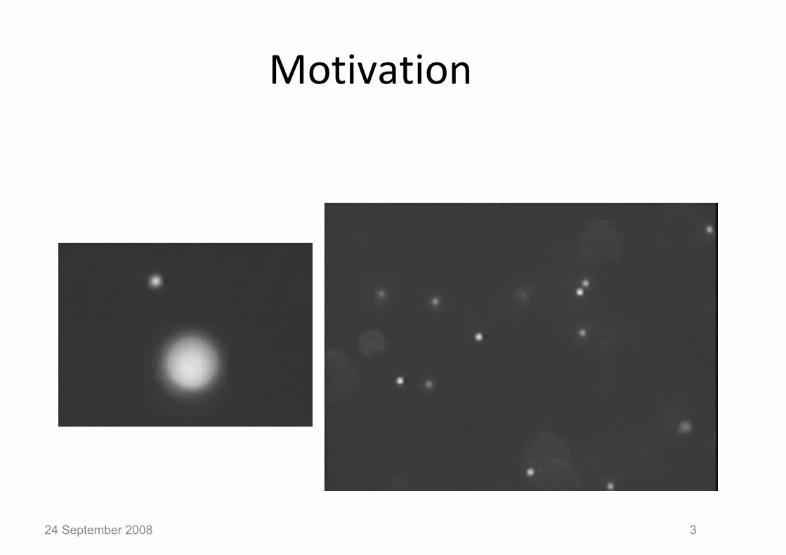
Motivation
24 September 2008 3
The art of doing research in physics
• We usually start with an observation of natural phenomenon
• We the have a nice idea on “How this phenomenon can be interpreted”
• We need model equations or simulation to build a solid base on the idea.
• Then the idea, started from an observation and moved on to a generic mathematical model, can become a prototype for interpreting many natural phenomena…. and this in the beauty of physics……
24 September 2008 4

Back on the “Brownian motion” : the idea
• Motion of small particles suspended in a fluid due to bombardment by molecules in thermal motion (the physicist)‐Einstein.
• Observed first by Jan Ingenhousz 1785, but was rediscovered by Brown in 1828.
• Pollen grains (from trees, plans) are organic substances with life in them, the erratic motion is expression of the power inherent to life (the botanologist)‐Brown
24 September 2008 5

Qualitative Idea
24 September 2008 6

Can we pose another question: How long it will take a drank man to go
from the bar to his house?
24 September 2008 7

Random walk in 2D
• Choose a random value in the interval
[‐1,1] and
24 September 2008 8
xΔ21y xΔ = ± − Δ

Question
• What will be the statistics of the distance <r(t_0)> at time t_0 after many repetitions?
24 September 2008 9

More….
• If the distance of the drank man from the bar to his house is 1000m and his step is 1m then you estimate the number of steps that are necessary and assuming that it takes several seconds for each step… you can estimate how long it will take him to reach home….
24 September 2008 10
2 21 1 2 2 3 3
2 21 1 2
( ..... )
( ) ....( ) .... 2( ) ....N N
N
R x y x y x y x y
x y x x
= Δ + Δ + Δ + Δ + Δ + Δ + + Δ + Δ
= Δ + Δ + + Δ Δ +

Mean free path
vλ τ=< >
24 September 2008 11
• A typical particle moving inside a fluid with density n of molecules with radius α will travel a mean distance
between collisions, <v> is the mean velocity and τ the
collision time. • Let us assume an ideal tube of length L and particle
collision cross section α inside the fluid. Typical particle will suffer
Collisions before exiting. From this relation we estimate the
mean free path
24N Lnπα=
2
14 n
λπα
=

Diffusion from random collisions
1 2
2 2
2 2 2
...
1( )3
n
i i j
z
z
N v N v
ζ ζ ζ
ζ ζ ζ
τ τ
= + + +
< >= < >+ < >< >
⎛ ⎞⎟⎜= < > = < > ⎟⎜ ⎟⎜⎝ ⎠
∑ ∑ ∑
24 September 2008 12
1 2
2 2
2 2 2
...
1( )3
n
i i j
z
z
z
N v N v
ζ ζ ζ
ζ ζ ζ
τ τ
= + + +
< >= < >+ < >< >
⎛ ⎞⎟⎜= < > = < > ⎟⎜ ⎟⎟⎜⎝ ⎠
∑ ∑ ∑
2 213
z v t Dtτ⎛ ⎞⎟⎜< >= < > =⎟⎜ ⎟⎟⎜⎝ ⎠
2 2 2
2
( ) ( / )( )
/ , / rms
R N r t r Dt
D r v
τ
τ τ λ
< >= < > = < > =
< > =∼

Mathematical formula for Brownian motion Langevin Formula
• Paul Langevin at 1908 modeled the Brownian motion m is the mass of the particle, v its Speed, γ=6πηα, η=dynamic viscosity, R(t)=randomly Fluctuating force
24 September 2008 13
( )ima F v R tγ= − +
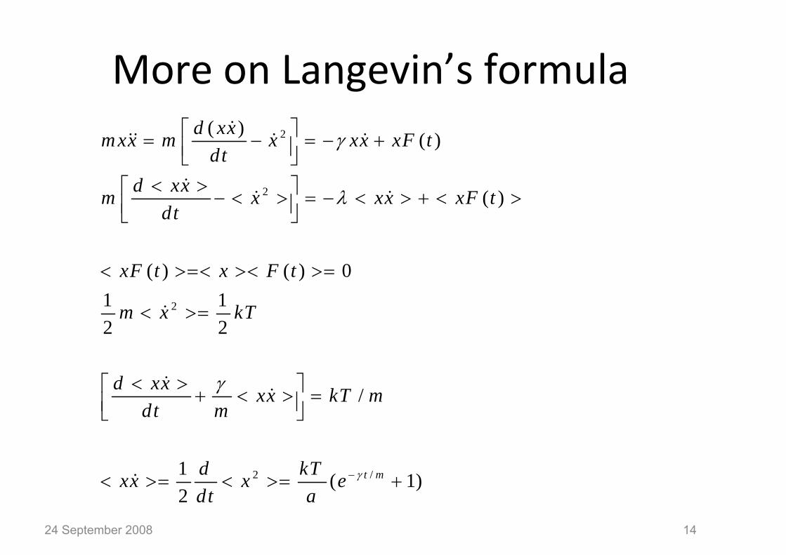
More on Langevin’s formula
24 September 2008 14
2
2
2
2 /
( ) ( )
( )
( ) ( ) 01 12 2
/
1 ( 1)2
t m
d xxmxx m x xx xF tdt
d xxm x xx xF tdt
xF t x F t
m x kT
d xx xx kT mdt m
d kTxx x edt a
γ
γ
λ
γ
−
⎡ ⎤= − = − +⎢ ⎥⎣ ⎦< >⎡ ⎤− < > = − < > + < >⎢ ⎥⎣ ⎦
< >=< >< >=
< >=
< >⎡ ⎤+ < > =⎢ ⎥⎣ ⎦
< >= < >= +

More on Langevin’s formula
24 September 2008 15
2 /2 (1 )t mkT mx t e γ
γ γ−⎡ ⎤
< >= − −⎢ ⎥⎣ ⎦

More on Langevin’s formula
• For
• Ballistic
24 September 2008 16
1
2 2
1
2
2 2
( / )
2( / )
23
3
t mkTx tm
t mNormal Diffusion
kT kTx t t
kTr x t Dt
γ
γ
γ
γ πηα
πηα
−
−
<<
< >=
>>
< >= =
< >= < >= =

24 September 2008 17
1. If the diffusion constant in atmosphere at 300 K isD = 10-5 m2/s, how far (in any direction) will perfume particles
diffuse in 1 minute?
r
Exercise 1: Perfume
2. Approximately how far up will the perfume diffuse in 1 minute?

24 September 2008 18
1. If the diffusion constant in atmosphere at 300 K is
D = 10-5 m2/s, how far (in any direction) will perfume particles diffuse in 1 minute?
r
Exercise 1: Perfume
( )( )
1/22rms
5 2
2
r r Dt
10 m /s 60s
6 10 m 6cm
−
−
≈ =
=
≈ × =
Approximately how far up will the perfume
diffuse in 1 minute?

The Diffusion equation
• Fick’s law
• The flux is proportional to the gradient in concentration
24 September 2008 19
nJ Dx
∂= −
∂
x x+∆x
2
2x x x
n n n nD Dt x x x+Δ
⎡ ⎤∂ ∂ ∂ ∂= − − =⎢ ⎥
∂ ∂ ∂ ∂⎢ ⎥⎣ ⎦
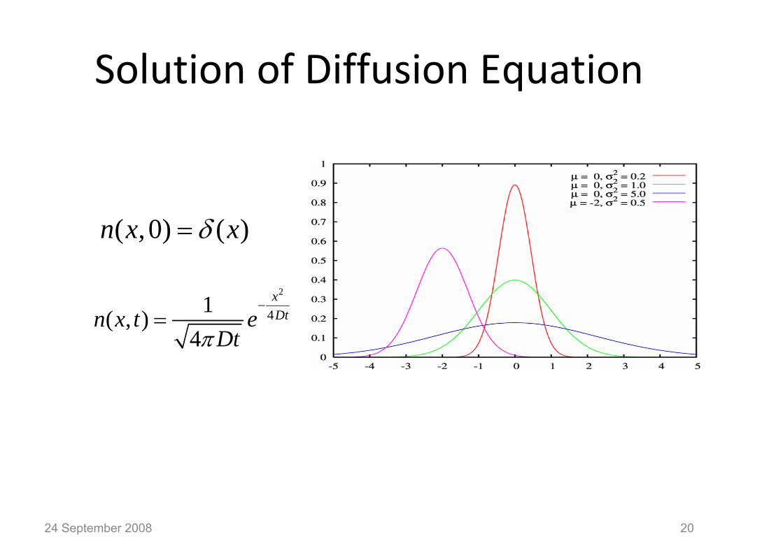
Solution of Diffusion Equation
24 September 2008 20
( ,0) ( )n x xδ=
2
41( , )4
xDtn x t e
Dtπ
−=

How to treat formally the classical RW
• Only position x of a particle is considered • Time step Δt constant (time plays dummy role, a simple counter) • Position of particle after n‐steps (at time tn = nΔt): xn
Δxi: jump increment: random x0: initial position
• Need to specify
• distribution of jump increments q(Δx): prob. to make a jump Δx
• → RW completely specified: problem: determine solution, i.e. probability P(x,tn) that a particle is at position x at time tn = n Δt
X0
X1
X2 Δx1 Δx2
21

How to treat formally the classical RW
• 1827: Brown observed that small particles (pollen grains) in a fluid followed an erratic zig‐zag path when seen under the microscope:now called Brownian motion – prototype of random walk.
• The solution of the RW is P(x,t), the probability for a particle to be at position x at time t, how to determine it ? • Problem treated by • 1900: Bachelier (PhD student of Poincare), modelling of stock market temporal evolution.
• 1905: Einstein, modelling of Brownian motion.
22
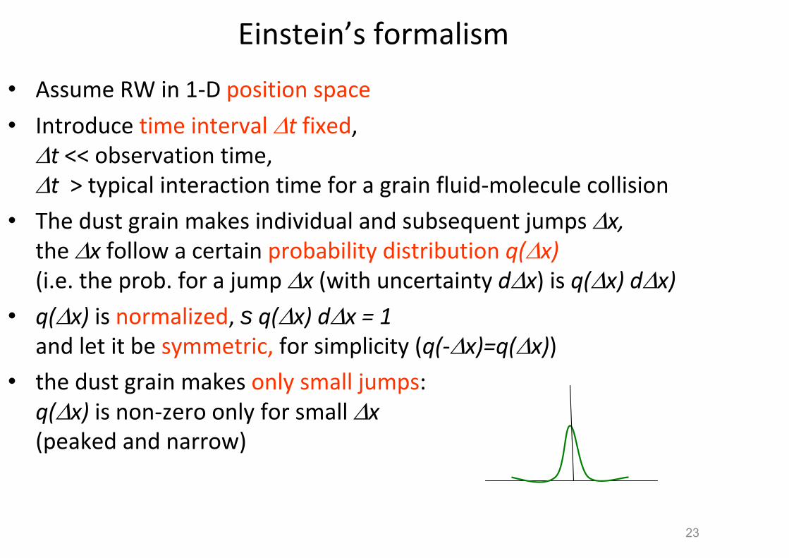
Einstein’s formalism
• Assume RW in 1‐D position space
• Introduce time interval Δt fixed, Δt << observation time, Δt > typical interaction time for a grain fluid‐molecule collision
• The dust grain makes individual and subsequent jumps Δx, the Δx follow a certain probability distribution q(Δx) (i.e. the prob. for a jump Δx (with uncertainty dΔx) is q(Δx) dΔx)
• q(Δx) is normalized, s q(Δx) dΔx = 1 and let it be symmetric, for simplicity (q(‐Δx)=q(Δx))
• the dust grain makes only small jumps: q(Δx) is non‐zero only for small Δx (peaked and narrow)
23

Einstein’s formalism, cont.
• We need to calculate P(x,t), the prob. for a particle to be at x at time t
• Assume we knew P(x, t‐Δt) at an earlier time t‐Δt, then P(x,t) = P(x‐Δx, t‐Δt) q(Δx) the prob. to be at x at time t equals the prob. to have been at x‐Δx at time t ‐ Δt ago and to have made a jump Δx in time Δt
• we still must sum over all possible Δx, RW equation in 1‐D → integral equation, to be solved for unknown P(x,t)
24

Einstein’s solution for P(x,t) • Einstein‐Bachelier equation
• Only small jumps: q(Δx) non‐zero only for small Δx, also Δt is small ) Taylor expand P(x‐Δx, t‐Δt),
• Insert
• Simplify
• Simple diffusion equation !
25
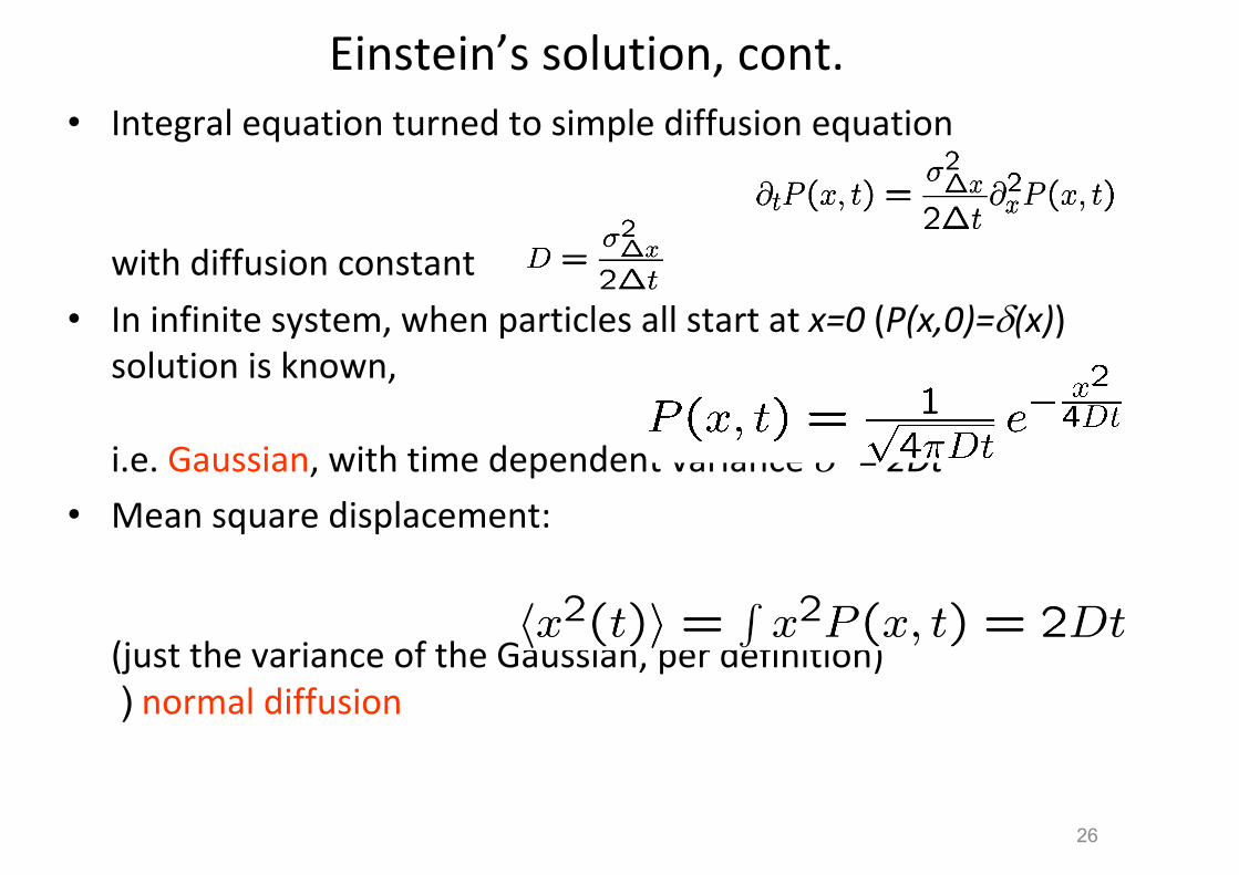
Einstein’s solution, cont. • Integral equation turned to simple diffusion equation
with diffusion constant
• In infinite system, when particles all start at x=0 (P(x,0)=δ(x)) solution is known, i.e. Gaussian, with time dependent variance σ2 = 2Dt
• Mean square displacement: (just the variance of the Gaussian, per definition) ) normal diffusion
26
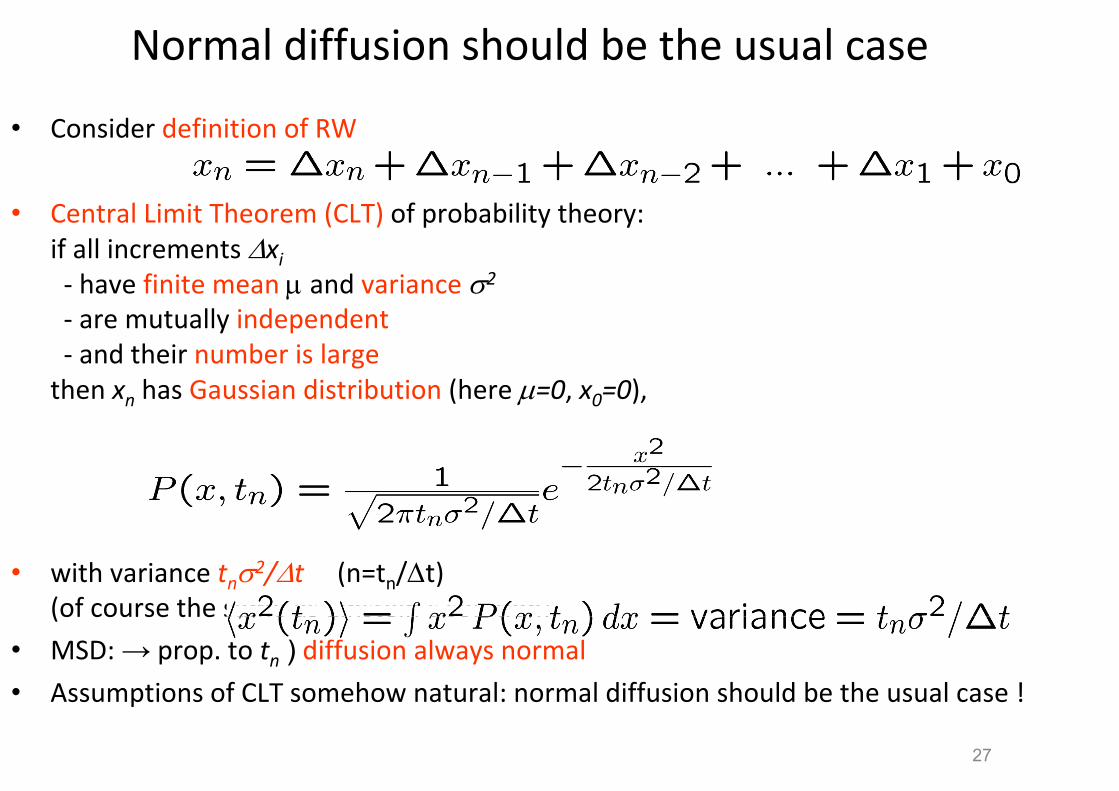
Normal diffusion should be the usual case
• Consider definition of RW
• Central Limit Theorem (CLT) of probability theory: if all increments Δxi ‐ have finite mean μ and variance σ2
‐ are mutually independent ‐ and their number is large then xn has Gaussian distribution (here μ=0, x0=0),
• with variance tnσ2/Δt (n=tn/Δt) (of course the same as Einstein’s solution)
• MSD: → prop. to tn ) diffusion always normal
• Assumptions of CLT somehow natural: normal diffusion should be the usual case !
27

Normal Diffusion
• 1. The mean square displacement
• 2. P(x,t)‐‐Gaussian (normal) distributions .
• 3. Diffusion equation
• 4. Langevin’s beautiful and simple formula can model the normal diffusion
24 September 2008 28
22 rr Dt or D
t< >
< >= =

Anomalous….Diffusion
24 September 2008 29

An experiment
24 September 2008 30

What we see
24 September 2008 31
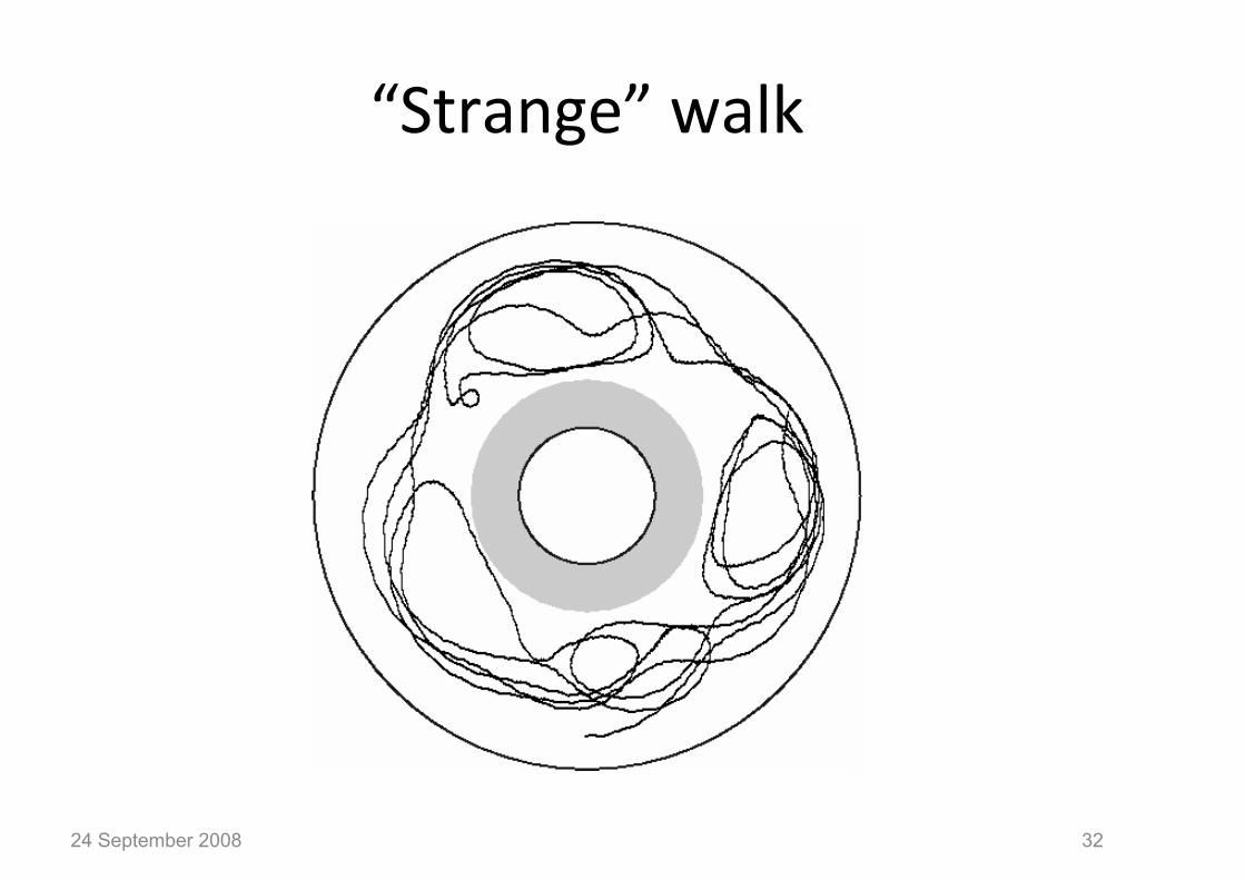
“Strange” walk
24 September 2008 32

Trajectories inside the annulus
24 September 2008 33
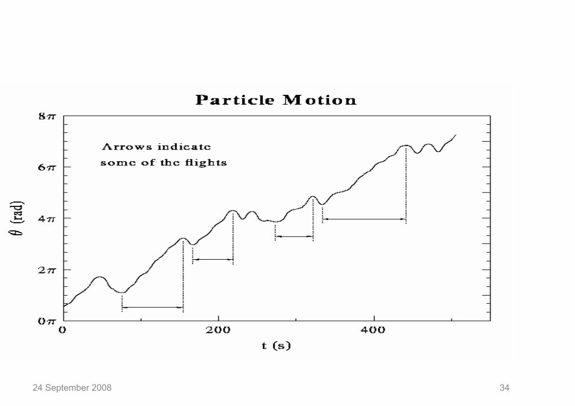
24 September 2008 34

24 September 2008 35
2 1.6r Dt< >∼
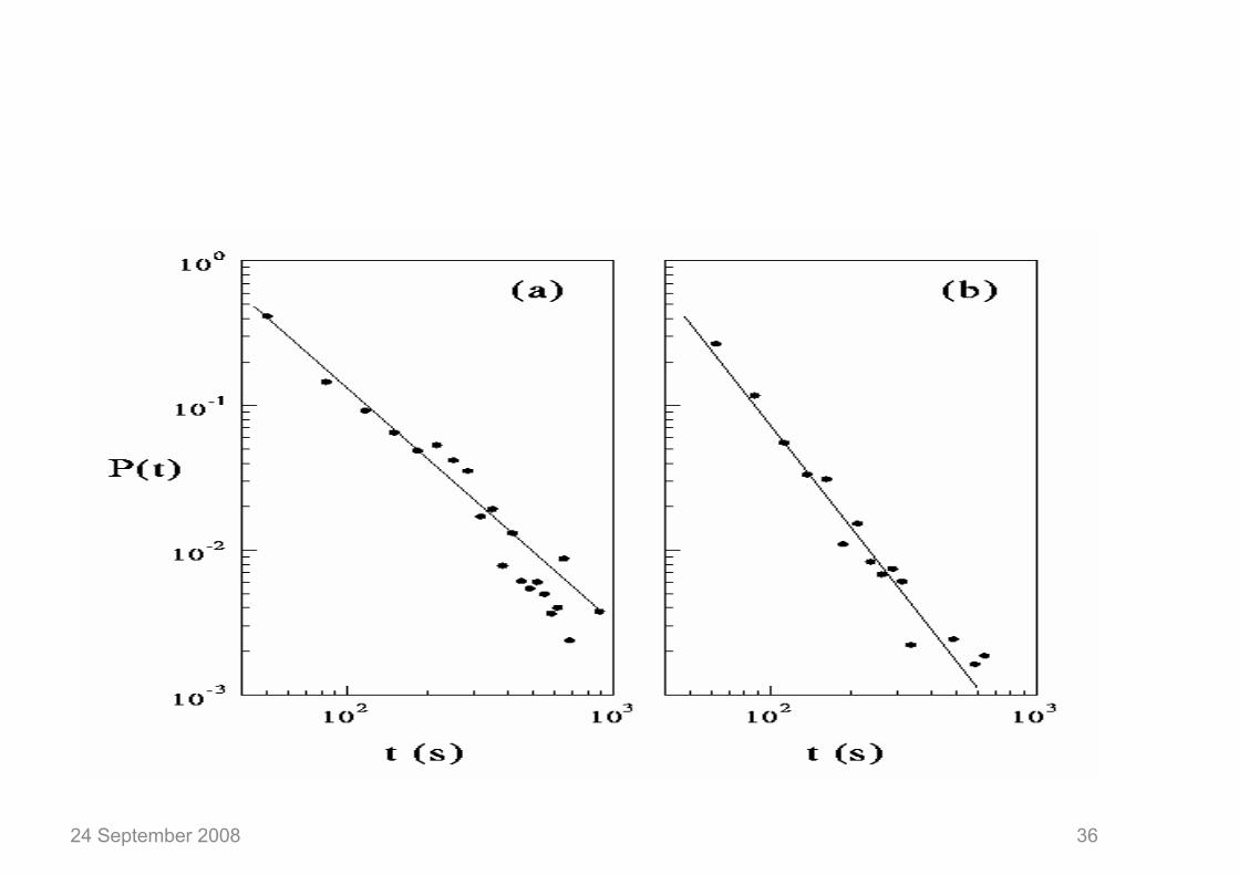
24 September 2008 36

Levy walks and anomalous diffusion
24 September 2008 37
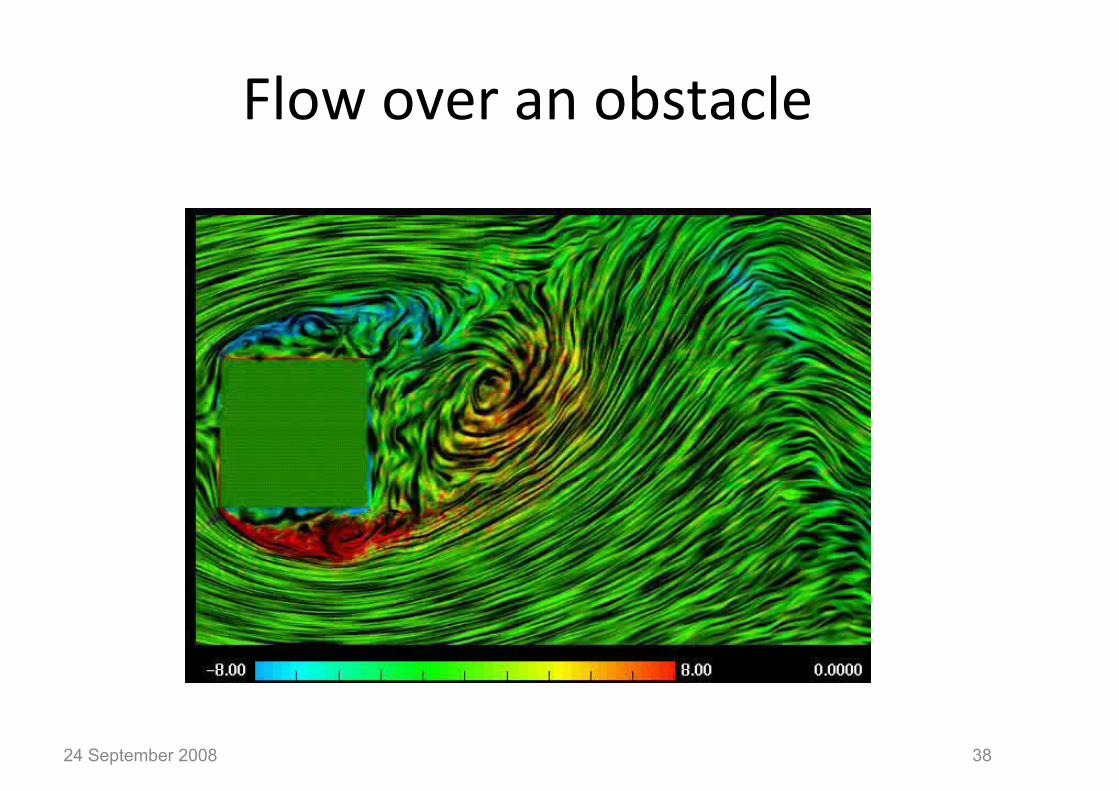
Flow over an obstacle
24 September 2008 38

Langevin type Equations
• Strange kinetics‐motion in a spatio‐temporal complex environment
24 September 2008 39
( , )idvm F v R x tdt
dx vdt
γ= − +
=

A ‘Turbulent’ Magnetic Field Model
A (x,t) = Σk ak cos(k•x − ω(k)t + φk)
⟨|ak|2⟩ ∼ (1+ kTSk)−ν
random φk
B = ∇ × A
E = – ∂t A + η(j) j
24 September 2008 40
threshold jc
J B∇×∼⇒

24 September 2008 41
Electromagnetic forces on charged particles
• We can follow the evolution of an ensemble of electrons in the presence of electromagnetic waves
( , )[ ( , ) ]dv v B x tm v q E x t
dt cdr vdt
γ ×= − + +
=
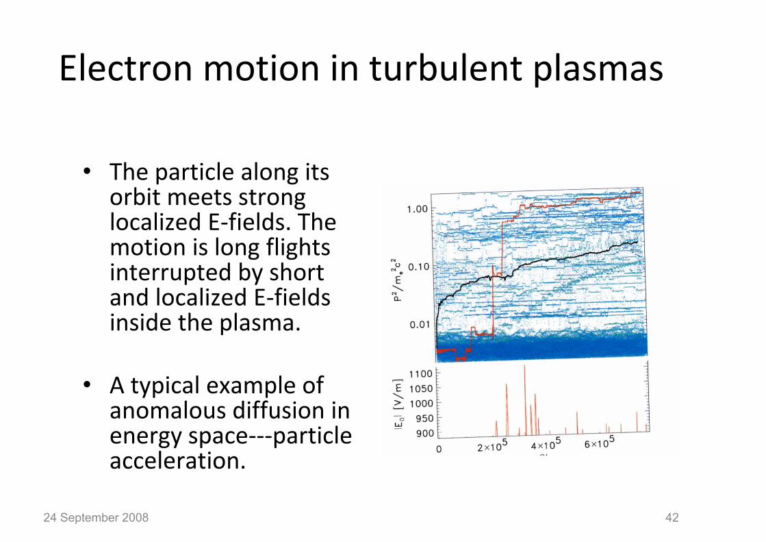
Electron motion in turbulent plasmas
• The particle along its orbit meets strong localized E‐fields. The motion is long flights interrupted by short and localized E‐fields inside the plasma.
• A typical example of
anomalous diffusion in energy space‐‐‐particle acceleration.
24 September 2008 42

Conditions for anomalous diffusion
• Central Limit Theorem (CLT) tries to make all diffusion normal
• For anomalous diffusion, we must violate at least one of its necessary conditions: (i) mean and/or variance of increments Δxi must be infinite, or (ii) increments Δxi must be mutually dependent, or (iii) the total number of increments must be small, or (iv) the time step Δt is not constant, anymore, but also random
• Point (iv) is what exactly is done in Continuous Time Random Walk (CTRW)
• Point (i) is realized by choice of particular distributions of increments q(Δx), the Levy‐distributions, with power‐law tails: q(Δx) » Δx‐α (for Δx large) (Levy distributions make though sense only in the frame of CTRW)
• Point (iii): small number of steps: less than 30 (with one step we would not talk about RW anymore)
• Point (ii) is an interesting possibility, could physically often be motivated – has it been tried ?
43

Continuous Time Random Walk (CTRW)
• Only position is considered (as in classical RW)
• Position of particle after n‐steps (at time tn): xn
Δxi: jump increment; x0: initial position → as in classical RW
• New in CTRW: time tn after n steps:
Δti : time needed to perform ith step: now random ) also tn random
• Need now to specify distribution of jump increments Δx and of temporal increments Δt : q(Δx,Δt): probability to make a jump Δx and to spend a time Δt in the jump
• → RW completely specified: problem: determine solution, i.e. prob. P(x,t) that particle is at position x at time t
44
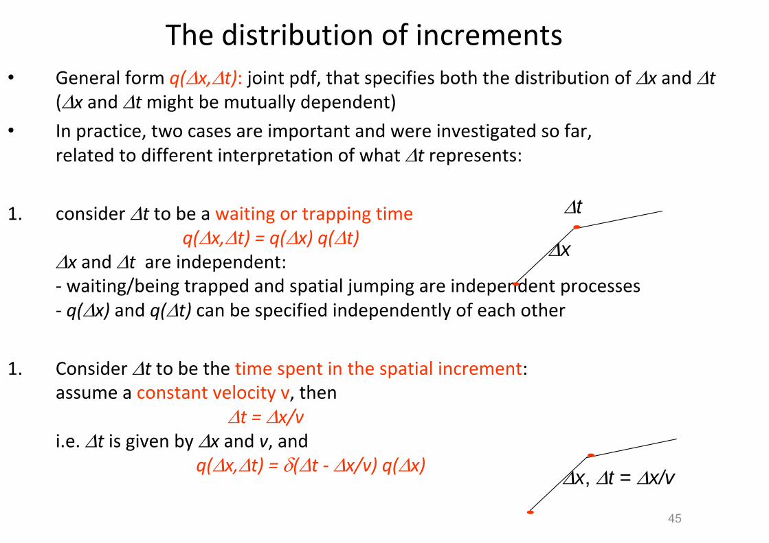
The distribution of increments • General form q(Δx,Δt): joint pdf, that specifies both the distribution of Δx and Δt
(Δx and Δt might be mutually dependent)
• In practice, two cases are important and were investigated so far, related to different interpretation of what Δt represents:
1. consider Δt to be a waiting or trapping time q(Δx,Δt) = q(Δx) q(Δt) Δx and Δt are independent: ‐ waiting/being trapped and spatial jumping are independent processes ‐ q(Δx) and q(Δt) can be specified independently of each other
1. Consider Δt to be the time spent in the spatial increment: assume a constant velocity v, then Δt = Δx/v i.e. Δt is given by Δx and v, and q(Δx,Δt) = δ(Δt ‐ Δx/v) q(Δx)
Δx Δt
Δx, Δt = Δx/v 45

The distribution of increments, cont.
• ‘Waiting/trapping model’: increments q(Δx) q(Δt) first version of CTRW historically introduced (1965, Montroll & Weiss) most published investigations/applications easiest to treat mathematically can though model only sub‐diffusion not useful for our intended applications in confined plasma
• ‘velocity model’: increments δ(Δt ‐ Δx/v) q(Δx) (introduced by Shlesinger & Klafter 1989) can model super‐diffusion we focus mostly on the velocity model, in the following
46

The CTRW equation I
• To treat the CTRW analytically, we need to derive its equation: waiting/trapping model: equation introduced in 1965 by Montroll and Weiss velocity model: equation introduced in 1989 by Shlesinger & Klafter
• Basically: generalize the Bachelier‐Einstein equation
• [Still, the equation must determine the probability P(x,t) for a particle to be at position x at time t]
• [CTRW can also be implemented numerically as a Monte‐Carlo simulation: let the computer trace the particles which make their random jumps]
47

The CTRW equation II • Generalize the Bachelier Einstein equation
• New symbol Q. Idea: connect Q(x,t) to Q(x‐Δ x,t‐Δ t) in the past:
Q(x,t) = Q(x‐Δx, t‐Δt) £ prob. to make a jump Δx in time Δt i.e. Q(x,t) = Q(x‐Δx, t‐Δt) £ δ(Δt ‐ Δx/v) q(Δx)
Prob. to be at x at time t equals probability to have been at time t ‐ Δt at position x ‐ Δx, and to have made a spatial jump Δx that took a time Δt
• Still need to sum over all possible Δx, Δt very close generalization of Bachelier‐Einstein
48

Still open problems on anomalous diffusion
• Interaction of non‐equilibrium media with particles
• Fractal forcing as drivers • Spatial inhomogeneities and diffusion • Diffusion in the entire phase space (x,v)
24 September 2008 49
2 1 sup1
ar t a er diffusiona sub diffusion
< > > −< −
∼

An open problem….Diffusion of Cosmic Rays through a fractal Universe: Moving through voids and localized action on gallaxies
24 September 2008 50

Charged particle’s voyage inside the universe
24 September 2008 51
Conclusions
• We have discussed the importance of random walk in nature and its relation to normal diffusion in stable systems.
• We have discussed a prototype of stochastic differential equations‐The Langevin equation.
• We introduced the notions of anomalous diffusion‐Levy flights and continuous random walk‐ all these are important for turbulent systems.
24 September 2008 52


