27
Normal Normal Distribution Distribution ch5 ch5
| Date post: | 19-Dec-2015 |
| Category: |
Documents |
| View: | 225 times |
| Download: | 2 times |

Normal DistributionNormal Distribution
ch5ch5

Normal DistributionNormal Distribution The random variable X has a The random variable X has a normal normal
distributiondistribution, N(μ, σ, N(μ, σ22), if its p.d.f. is defined ), if its p.d.f. is defined byby where the mean μ (-∞, ∞), and variance σ∈where the mean μ (-∞, ∞), and variance σ∈ 22 (0, ∞).∈(0, ∞).∈
If Z is N(0, 1), Z is called as a standard If Z is N(0, 1), Z is called as a standard normal distribution.normal distribution.
M(t)=
M’(t)=
E(X)=

ExamplesExamples Ex.5.2-3: If Z is N(0,1), then from Table Va on p.686,Ex.5.2-3: If Z is N(0,1), then from Table Va on p.686,
Φ(1.24)=P(Z 1.24)=0.8925, ≦Φ(1.24)=P(Z 1.24)=0.8925, ≦ P(P(1.24 Z 2.37)=Φ (2.37)-Φ (1.24)=0.9911-0.8925=0.0986≦ ≦1.24 Z 2.37)=Φ (2.37)-Φ (1.24)=0.9911-0.8925=0.0986≦ ≦ P(-2.37 Z -1.24)= P(1.24 Z 2.37)=0.0986≦ ≦ ≦ ≦P(-2.37 Z -1.24)= P(1.24 Z 2.37)=0.0986≦ ≦ ≦ ≦
From Table Vb (right-tail) on p.687, (the negative z is deriveFrom Table Vb (right-tail) on p.687, (the negative z is derived from –Z)d from –Z) P(ZP(Z>1.24)=0.1075 P(Z -2.14)=P(Z 2.14)=0.0162≦ ≧>1.24)=0.1075 P(Z -2.14)=P(Z 2.14)=0.0162≦ ≧
Ex.5.2-4: If Z is N(0,1), then find a & b from Table Va & Vb.Ex.5.2-4: If Z is N(0,1), then find a & b from Table Va & Vb. P(Z a)=0.9147 => a=1.37≦P(Z a)=0.9147 => a=1.37≦ P(Z b)=0.0526 => b=1.62≧P(Z b)=0.0526 => b=1.62≧
Percentiles:Percentiles: The 100(1-α) percentile is The 100(1-α) percentile is ZZαα, where P(Z Z≧, where P(Z Z≧ αα)=α=P(Z -Z≦)=α=P(Z -Z≦ αα) Z) Z1-α1-α=-Z=-Zαα
(the upper 100αpercent point)(the upper 100αpercent point)
The 100p percentile is πThe 100p percentile is πpp, where P(X, where P(X≦≦ππpp)=p )=p p=1-α =>πp=1-α =>πpp=Z=Z1-p1-p=-Z=-Zpp

Conversion: N(μ,σConversion: N(μ,σ22) ) ⇒ N(0,1)) ) ⇒ N(0,1) Thm5.2-1: If X is N(μ,σThm5.2-1: If X is N(μ,σ22), then Z=(X-μ)/σis N(0,1).), then Z=(X-μ)/σis N(0,1).
Usage:Usage:
Ex.5.2-6: X is N(3,16). Ex.5.2-6: X is N(3,16).
Ex.5.2-7: X is N(25,36). Find c such that P(|X-25|≤c) Ex.5.2-7: X is N(25,36). Find c such that P(|X-25|≤c) =0.9544.=0.9544.
Within 2*σabout the mean, X and Z share the same the Within 2*σabout the mean, X and Z share the same the probability.probability.
P(4X8)

Conversion N(μ,σConversion N(μ,σ22) ⇒ χ) ⇒ χ22(1)(1) Thm5.2-2: If X is N(μ,σThm5.2-2: If X is N(μ,σ22), then V=[(X-μ)/σ]), then V=[(X-μ)/σ]22=Z=Z22is χis χ22(1).(1).
Pf: V=ZPf: V=Z22, Z is N(0,1). Then G(v) of V is, Z is N(0,1). Then G(v) of V isG(V)G(V)
Ex.5.2-8: If Z is N(0,1), k=? So Ex.5.2-8: If Z is N(0,1), k=? So From the chi-square table with r=1, kFrom the chi-square table with r=1, k22=3.841, so k=1.96=3.841, so k=1.96..
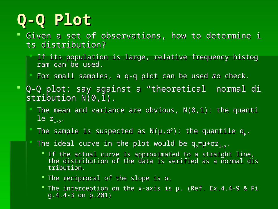
Q-Q PlotQ-Q Plot Given a set of observations, how to determine its distribuGiven a set of observations, how to determine its distribu
tion?tion? If its population is large, relative frequency histogram can be useIf its population is large, relative frequency histogram can be use
d.d.
For small samples, a q-q plot can be used to check.For small samples, a q-q plot can be used to check.
Q-Q plot: say against a “theoretical” normal distribution NQ-Q plot: say against a “theoretical” normal distribution N(0,1).(0,1). The mean and variance are obvious, N(0,1): the quantile zThe mean and variance are obvious, N(0,1): the quantile z1-p1-p..
The sample is suspected as N(μ,σThe sample is suspected as N(μ,σ22): the quantile q): the quantile qpp..
The ideal curve in the plot would be qThe ideal curve in the plot would be qpp=μ+σz=μ+σz1-p1-p..
If the actual curve is approximated to a straight line, the distribution If the actual curve is approximated to a straight line, the distribution of the data is verified as a normal distribution.of the data is verified as a normal distribution.
The reciprocal of the slope is σ.The reciprocal of the slope is σ.
The interception on the x-axis is μ. (Ref. Ex.4.4-9 & Fig.4.4-3 on p.2The interception on the x-axis is μ. (Ref. Ex.4.4-9 & Fig.4.4-3 on p.201)01)

Statistics on Normal Statistics on Normal
DistributionsDistributions Thm5.3-1: XThm5.3-1: X11,…,X,…,Xn n are the outcomes on a random sample of are the outcomes on a random sample of
size n from the normal distribution N(μ,σsize n from the normal distribution N(μ,σ22). ). The distribution of the sample mean is N(μ,σThe distribution of the sample mean is N(μ,σ22/n)./n). Pf:Pf:
Thm5.3-2: ZThm5.3-2: Z11,…,Z,…,Znn are independent and all have N(0,1); The are independent and all have N(0,1); The
n, W=Zn, W=Z1122+…+Z+…+Znn
22is χis χ22(n). (n).
Pf: Pf:
Thm5.2-2: If X is N(μ,σThm5.2-2: If X is N(μ,σ22), then V=[(X-μ)/σ]), then V=[(X-μ)/σ]22=Z=Z2 2 is χis χ22(1).(1).Thm4.6-3: Y=XThm4.6-3: Y=X11+…+X+…+Xn n is χis χ22(r(r11+…+r+…+rnn)= χ)= χ22(n) in this case. (n) in this case.
MX(t)

Example Example Fig.5.3-1: p.d.f.s of means of samples from N(50,16).Fig.5.3-1: p.d.f.s of means of samples from N(50,16).
is N(50, 16/n).is N(50, 16/n).

Theoretical Mean and Sample MeanTheoretical Mean and Sample Mean Cly5.3-1: ZCly5.3-1: Z11,…,Z,…,Zn n are independent and have N(μare independent and have N(μii,σ,σii
22),i=1..n; ),i=1..n;
Then, W=[(ZThen, W=[(Z11-μ-μ11)/σ)/σii22]]22+…+[(Z+…+[(Znn-μ-μnn)/σ)/σnn
22]]2 2 is χis χ22(n). (n).
Thm5.3-3: XThm5.3-3: X11,…,X,…,Xn n are the outcomes on a random sample are the outcomes on a random sample
of size n from the normal distribution N(μ,σof size n from the normal distribution N(μ,σ22). Then,). Then, The sample mean & variance aThe sample mean & variance a
re indep. re indep.
is is χχ22(n-1)(n-1)Pf: Pf: (a) omitted; (b):(a) omitted; (b):
As theoretical mean is replaced by the sample mean, one degree of freedom As theoretical mean is replaced by the sample mean, one degree of freedom is lost! is lost!
MV(t)

Linear Combinations of N(μ,σLinear Combinations of N(μ,σ22)) Ex5.3-2: XEx5.3-2: X11,X,X22,X,X33,X,X4 4 are a random sample of size 4 from the nare a random sample of size 4 from the n
ormal distribution N(76.4,383). Then ormal distribution N(76.4,383). Then
P(0.711P(0.711W W 7.779)=0.9-0.05=0.85, P(0.352 7.779)=0.9-0.05=0.85, P(0.352 V V 6.251)=0.9-0.05=0.856.251)=0.9-0.05=0.85
Thm5.3-4: If XThm5.3-4: If X11,…,X,…,Xn n are n mutually indep. normal variables ware n mutually indep. normal variables w
ith means μith means μ11,…,μ,…,μn n & variances σ& variances σ1122,…,σ,…,σnn
22, then the linear functi, then the linear functi
onon has the normal distribution has the normal distribution Pf: By moment-generating function, … Pf: By moment-generating function, …
Ex5.3-3: XEx5.3-3: X11:N(693.2,22820) and X:N(693.2,22820) and X22:N(631.7,19205) are indep. :N(631.7,19205) are indep.
Find P(XFind P(X11>X>X22) ) Y=XY=X11-X-X2 2 is N(61.5,42025). is N(61.5,42025).
P(XP(X11>X>X22)=P(Y>0)=)=P(Y>0)=

Box-Muller Transformation Box-Muller Transformation Ex5.3-4: XEx5.3-4: X1 1 and Xand X2 2 have indep. Uniform distributions U(0,1). have indep. Uniform distributions U(0,1).
Consider Consider
Two indep. U(0,1) two indep. N(0,1)!! ⇒Two indep. U(0,1) two indep. N(0,1)!! ⇒

Distribution Function TechniqueDistribution Function Technique Ex.5.3-5: Z is N(0,1), U is χEx.5.3-5: Z is N(0,1), U is χ22(r), Z and U are independent.(r), Z and U are independent.
The joint p.d.f. of Z and U isThe joint p.d.f. of Z and U is
χ2(r+1)

Student’s T DistributionStudent’s T Distribution Gossett, William Sealy published “t-test” in Biometrika1908 Gossett, William Sealy published “t-test” in Biometrika1908
to measure the confidence interval, the deviation of “small to measure the confidence interval, the deviation of “small samples” from the “real”. samples” from the “real”. Suppose the underlying distribution is normal with unknown σSuppose the underlying distribution is normal with unknown σ22. .
Fig.5.3-2: The T p.d.f. Fig.5.3-2: The T p.d.f. becomes closer to the becomes closer to the N(0, 1) p.d.f. as the numbeN(0, 1) p.d.f. as the number r of degrees of freedom incrof degrees of freedom increases.eases.
ttαα(r) (r) is the 100(1-α) percentile, or the upper 100αpercent point. [Table VI, p.658] is the 100(1-α) percentile, or the upper 100αpercent point. [Table VI, p.658]
f(t)=
Only depends on r!

Examples Examples Ex: Suppose T has a t distribution with r=7. Ex: Suppose T has a t distribution with r=7.
From Table VI on p.688, From Table VI on p.688,
Ex: Suppose T has a t distribution with r=14.Ex: Suppose T has a t distribution with r=14. Find a constant c, such that P(|T|<c)=0.9 Find a constant c, such that P(|T|<c)=0.9 From Table VI on p.688, From Table VI on p.688,

Central Limit Theorem Central Limit Theorem Ex4.6-2: XEx4.6-2: X11,…,X,…,Xn n are a random sample of size n from a distriare a random sample of size n from a distri
bution with mean μand variance σbution with mean μand variance σ22; then ; then
The sample mean: The sample mean:
Thm5.4-1: (Central Limit Theorem) If is the mean of a randThm5.4-1: (Central Limit Theorem) If is the mean of a random sample Xom sample X11,…,X,…,Xn n of size n from some distribution with a finiof size n from some distribution with a fini
te mean μand a finite positive variance σte mean μand a finite positive variance σ22, then the distributio, then the distribution ofn of
is N(0, 1) in the limit as n →∞. Even if Xis N(0, 1) in the limit as n →∞. Even if X ii is not N(μ,σ is not N(μ,σ22).).
W= if n is large
W

More ExamplesMore Examples Ex: Let denote the mean of a random sample of size Ex: Let denote the mean of a random sample of size
n=15 from the distribution whose p.d.f. is f(x)=3xn=15 from the distribution whose p.d.f. is f(x)=3x22/2, -1<x<1./2, -1<x<1. μ=0, σμ=0, σ22=3/5.=3/5.
Ex5.4-2: Let XEx5.4-2: Let X11,…,X,…,X20 20 be a random sample of size 20 from be a random sample of size 20 from
the uniform distribution U(0,1). the uniform distribution U(0,1). μ=½, σμ=½, σ22=1/12; Y=X=1/12; Y=X11+…+X+…+X2020..
Ex5.4-3: Let denote the mean of a random sample of Ex5.4-3: Let denote the mean of a random sample of size n=25 from the distribution whose p.d.f. is f(x)=xsize n=25 from the distribution whose p.d.f. is f(x)=x33/4, /4, 0<x<20<x<2 μ=1.6, σμ=1.6, σ22=8/75.=8/75.

How large of size n is sufficient?How large of size n is sufficient? If n=25, 30 or larger, the approximation is generally goodIf n=25, 30 or larger, the approximation is generally good. .
If the original distribution is symmetric, unimodal and of continuous tyIf the original distribution is symmetric, unimodal and of continuous type, n can be as small as 4 or 5. pe, n can be as small as 4 or 5.
If the original is like normal, n can be lowered to 2 or 3. If the original is like normal, n can be lowered to 2 or 3. If it is exactly normal, n=1 or more is just good. If it is exactly normal, n=1 or more is just good.
However, if the original is highly skew, n must be quite large. However, if the original is highly skew, n must be quite large.
Ex5.4-4: Let XEx5.4-4: Let X11,…,X,…,X4 4 be a random sample of size 4 from the be a random sample of size 4 from the
uniform distribution U(0,1) with p.d.f. f(x)=1, 0<x<1uniform distribution U(0,1) with p.d.f. f(x)=1, 0<x<1. . μ=½, σμ=½, σ22=1/12; Y=X=1/12; Y=X11+X+X22..
Y=XY=X11+…+X+…+X44..

Graphic Illustration Graphic Illustration Fig.5.4-1: Sum of n U(0, 1) R.V.s Fig.5.4-1: Sum of n U(0, 1) R.V.s
N( n(1/2), n(1/12) ) p.d.f. N( n(1/2), n(1/12) ) p.d.f.

Skew DistributionsSkew Distributions Suppose f(x) and F(x) are the p.d.f. and distribution function Suppose f(x) and F(x) are the p.d.f. and distribution function
of a random variable X with mean μ and variance σof a random variable X with mean μ and variance σ22. .
Ex5.4-5: Let XEx5.4-5: Let X11,…,X,…,Xn n be a random sample of size n from a chbe a random sample of size n from a ch
i-square distribution χi-square distribution χ22(1). (1). Y=XY=X11+…+X+…+Xnn is χ is χ22(n), E(Y)=n, Var(Y)=2n. (n), E(Y)=n, Var(Y)=2n.
n=20 or 100 n=20 or 100 →→N( , ). N( , ).

Graphic Illustration Graphic Illustration Fig.5.4-2: The p.d.f.s of sums of χFig.5.4-2: The p.d.f.s of sums of χ22(1), transformed so that (1), transformed so that
their mean is equal to zero and variance is equal to one, their mean is equal to zero and variance is equal to one, becomes closer to the N(0, 1) as the number of degrees of becomes closer to the N(0, 1) as the number of degrees of freedom increases. freedom increases.

Simulation of R.V. X with f(x) & F(x)Simulation of R.V. X with f(x) & F(x) Random number generator will produce values y’s for U(0,1). Random number generator will produce values y’s for U(0,1).
Since F(x)=U(0,1)=Y, x=FSince F(x)=U(0,1)=Y, x=F-1-1(y) is an observed or simulated value of X. (y) is an observed or simulated value of X.
Ex.5.4-6: Let XEx.5.4-6: Let X11,…,X,…,Xn n be a random sample of size n from the be a random sample of size n from the
distribution with f(x), F(x), mean μand variance σdistribution with f(x), F(x), mean μand variance σ22.. 1000 random samples are simulated to compute the values of W.1000 random samples are simulated to compute the values of W. A histogram of these values are grouped into 21 classes of equal widtA histogram of these values are grouped into 21 classes of equal widt
h.h.f(x)=(x+1)/2, F(x)=(x+1)f(x)=(x+1)/2, F(x)=(x+1)22/4, f(x)=3x/4, f(x)=3x22/2, F(x)=(x/2, F(x)=(x33+1)/2, +1)/2,
-1<x<1; μ=1/3, σ-1<x<1; μ=1/3, σ22=2/9. -1<x<1; μ=0, σ=2/9. -1<x<1; μ=0, σ22=3/5.=3/5.
N(0,1)N(0,1)

Approximation of Discrete Approximation of Discrete
DistributionsDistributions Let XLet X11,…,X,…,Xn n be a random sample from a be a random sample from a Bernoulli Bernoulli distributidistributi
on with μ=p and σon with μ=p and σ22=npq, 0<p<1.=npq, 0<p<1. Thus, Y=XThus, Y=X11+…+X+…+Xn n is is binomial binomial b(n,p). →N(np,npq) as n →∞. b(n,p). →N(np,npq) as n →∞.
Rule: n is “sufficiently large” if npRule: n is “sufficiently large” if np5 and nq5 and nq5. 5. If p deviates from 0.5 (skew!!), n need to be larger. If p deviates from 0.5 (skew!!), n need to be larger.
Ex.5.5-1: Y, b(10,1/2), Ex.5.5-1: Y, b(10,1/2), can be approximated by can be approximated by N(5,2.5). N(5,2.5).
Ex.5.5-2: Y, b(18,1/6), Ex.5.5-2: Y, b(18,1/6), can be hardly approx. by can be hardly approx. by N(3,2.5), 3<5. ∵N(3,2.5), 3<5. ∵

Another ExampleAnother Example Ex5.5-4: Y is b(36,1/2).Ex5.5-4: Y is b(36,1/2).
Correct Probability: Correct Probability:
Approximation of Binomial Distribution b(n,p): Approximation of Binomial Distribution b(n,p):
Good approx.!

Approximation of Poisson Approximation of Poisson
DistributionDistribution Approximation of a Poisson Distribution Y with mean λ: Approximation of a Poisson Distribution Y with mean λ:
Ex5.5-5: X that has a Poisson distribution with mean 20 can Ex5.5-5: X that has a Poisson distribution with mean 20 can be seen as the sum Y of the observations of a random be seen as the sum Y of the observations of a random sample of size 20 from a Poisson distribution with mean 1.sample of size 20 from a Poisson distribution with mean 1.
Correct Probability: Correct Probability:
Fig.5.5-3: Normal approx. of the Poisson Probability Histogram

Bivariate Normal DistributionBivariate Normal Distribution The joint p.d.f of X : N(μThe joint p.d.f of X : N(μXX,σ,σXX
22)and Y : N(μ)and Y : N(μYY,σ,σYY22) is) is
Therefore,Therefore,
A linear function of x. A constant w.r.t. x.

ExamplesExamples Ex.5.6-1:Ex.5.6-1:
Ex.5.6-2Ex.5.6-2

Bivariate Normal:ρ=0 ⇒ IndependenceBivariate Normal:ρ=0 ⇒ Independence Thm5.6-1: For X and Y with a bivariate normal distribution wThm5.6-1: For X and Y with a bivariate normal distribution w
ith ρ, X and Y are independent iffρ=0.ith ρ, X and Y are independent iffρ=0. So are trivariate and multivariate normal distributions.So are trivariate and multivariate normal distributions.
When ρ=0,When ρ=0,


![Type of dual superconductivity for the SU 2 Yang–Mills theory · [19,20] of the lattice Yang–Mills theory by decomposing the gauge field Ux,μ into Vx,μ and Xx,μ, Ux,μ = Xx,μVx,μ,](https://static.documents.pub/doc/80x56/5f6e0973d5ede40ac408ebfa/type-of-dual-superconductivity-for-the-su-2-yangamills-theory-1920-of-the-lattice.jpg)


![Linear Algebra and its Applications · 2016. 12. 16. · Laplacian eigenvalues are all real and nonnegative [1]. The set of all N Laplacian eigenvalues μ N = 0 μ N−1 ··· μ](https://static.documents.pub/doc/80x56/5fc39bf132385c3e370ab1c6/linear-algebra-and-its-applications-2016-12-16-laplacian-eigenvalues-are-all.jpg)


![Chapter 2 (part 3) Bayesian Decision Theory · vectors are generated by two normal distributions sharing the same covariance matrix and the mean vectors are μ 1 = [0, 0]t, μ 2=](https://static.documents.pub/doc/80x56/5f9dd58d1957941232557212/chapter-2-part-3-bayesian-decision-theory-vectors-are-generated-by-two-normal.jpg)