E . A . H E R M A N

DIE CASTING PROCESS CONTROL

PUBLICATION: E-410

Average

Triangle Approximating Histogram

R/3R/3R/3R

NORTH AMERICAN DIE CASTING ASSOCIATION

Die Casting Process Control

E.A. Herman

ii

Although great care has been taken to provide accurate and current information, neither the author(s) nor the publisher, nor anyone else associated with this publication, shall be liable for any loss, damage or liability directly or indirectly caused or alleged

to be caused by this book. The material contained herein is not intended to provide specific advice or recommendations for any specific situation. Any opinions expressed by the author(s) are not necessarily those of NADCA. Trademark notice: Product or corporate names may be trademarks or registered trademarks and are used only for identification and explanation without intent

to infringe nor endorse the product or corporation. © 2012 by North American Die Casting Association, Arlington Heights, Illinois. All Rights Reserved. Neither this book nor any part may be reproduced or transmitted in any form or by any means, elec-

tronic or mechanical, including photocopying, microfilming, and recording, or by any information storage and retrieval system, without permission in writing form the publisher.

First Printing 1988Second Printing 1991Major Revision 2003

Minor Edits Spring 2012

iii

Preface . . . . . . . . . . . . . . . . . . . . . . . . . . . . . . . . . . . . . . . . . . . . . . . . . . . . . . . . . . . . . . . . . . . . . . . . . . . . 2

Chapter 1: Introduction to Control Theory . . . . . . . . . . . . . . . . . . . . . . . . . . . 5

Chapter 2: Measuring Process Capability . . . . . . . . . . . . . . . . . . . . . . . . . . . . . 9

Chapter 3: Statistical Process Control . . . . . . . . . . . . . . . . . . . . . . . . . . . . . . . . . 17

Chapter 4: Holding Furnace Temperature . . . . . . . . . . . . . . . . . . . . . . . . . . . 22

Chapter 5: Plunger Velocity & Force . . . . . . . . . . . . . . . . . . . . . . . . . . . . . . . . . . 26

Chapter 6: Clamping Force . . . . . . . . . . . . . . . . . . . . . . . . . . . . . . . . . . . . . . . . . . . . . . . 34

Chapter 7: Die Temperature . . . . . . . . . . . . . . . . . . . . . . . . . . . . . . . . . . . . . . . . . . . . . . 42

Chapter 8: Release Material . . . . . . . . . . . . . . . . . . . . . . . . . . . . . . . . . . . . . . . . . . . . . . 48

Chapter 9: Casting Ejection Temperature . . . . . . . . . . . . . . . . . . . . . . . . . . . 52

Chapter 10: Cycle Timing . . . . . . . . . . . . . . . . . . . . . . . . . . . . . . . . . . . . . . . . . . . . . . . . 57

Chapter 11: Mechanical Die System . . . . . . . . . . . . . . . . . . . . . . . . . . . . . . . . . . . 61

Chapter 12: Implementation . . . . . . . . . . . . . . . . . . . . . . . . . . . . . . . . . . . . . . . . . . . . . 67

Chapter 13: Process Potential . . . . . . . . . . . . . . . . . . . . . . . . . . . . . . . . . . . . . . . . . . . . 70

References . . . . . . . . . . . . . . . . . . . . . . . . . . . . . . . . . . . . . . . . . . . . . . . . . . . . . . . . . . . . . . . . . . . . . . 73

Table of Contents

Die Casting Process, Engineering and Control2

The die casting industry has now progressed to where the degree of process control that can be routinely applied is at least ten times (and possibly 100 times) that of just a few years ago. The previous edition of this book started here by saying the industry was in a “revolution of process control”. That revolution has come and gone, and practical, in fact necessary, controls must now be applied to the process if the die caster is to compete in the market place. Traditionally the control of the process was accom­plished by the machine operator. He would inspect the cast ings as he made them and then make adjustments to the oper ation of the process. The success of any particular operation depended substantially upon the skill of the operator and entirely on the fidelity of his physical senses. Such manual feed back control loops do not have sufficient sensi tivity, responsiveness or reliabil­ity to maximize the potential of the die casting process.

The modern die casting manager knows that to realize the full potential of the process, he must have both electro­hydraulic­mechanical feed­back control devices and the process engineer­ing and operating skills to use those devices properly. This book and the associated certificate earning NADCA course have been created to help develop those skills. Each major process variable is identified, its natural behavior described, and the required control scheme is defined.

For definitive cause­and­effect relationships between the process ing variables and casting quality, the reader is referred to other NADCA courses such as Heat Flow, Die Casting Dies: Designing, Dimensional Re peatability, Gating and Metallurgy. This book does not describe the set up, calibra­tion or maintenance of the process controlling instruments and/or equipment. That information must be ob tained from the equipment manufacturers. This book does not evaluate

Preface

competitive brands of control equipment. Any specific equip­ment used to illustrate a point was selected only because of the suitability and availability of the print able material as this book was being written. Once a suitable illustration was found, no effort was made to search out oth ers. This book does not describe die casting machine functions, maintenance or fault diagnosis. The assumption is made that the reader knows how the machine and die systems work and that everything is working properly and can therefore be adjusted as necessary to achieve the desired results. The mechanics and engineering design criteria for the various machine systems are presented in the NADCA course on Machine Systems. This book does not explain how to determine what the “set point” operating values of the various variables should be. Other NADCA textbooks and courses such as Gating, Engineering Die Casting Dies and Engineering Die Cooling Systems show how to make those processing set point calculations. The previous edition went into considerable detail on how to establish some, but not all, of the set points and was accordingly titled “Process Engineering and Control.” Some instruments used for controlling the process are equally useful for diagnos ing improper functioning of the die casting machine. So when a particular type of instrumentation is discussed in this book, the reader should be aware that there could be other uses for it.

The purpose of this book is to show the processing engi neer and operating technician what type of control method is applicable to each of the die casting machine/die/process systems, how to measure the performance of each critical variable, compare actual performance to the desired and to adjust the actual per­formance to meet the desired. The reader will find this edition more definitive and focused than the previous editions.

Die Casting Process, Engineering and Control

C H A P T E R

5

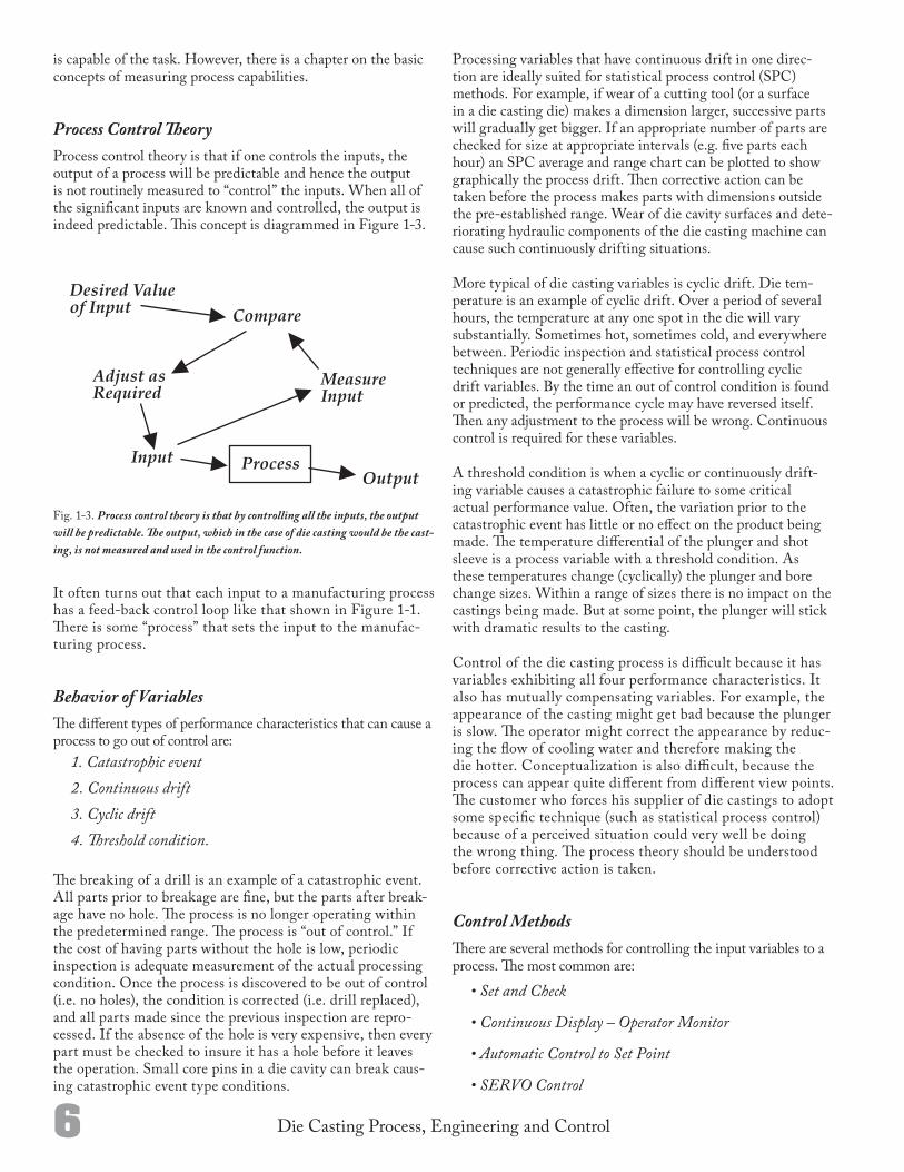
lack of a coherent theory of the causes and effects relationships between spe cific adjustments, machine/process performance and casting quality. The machine operator did not have all the tools (both physical and informational) that he needed. The results have been a catch­as­catch­can situation where both good and bad castings are produced on a somewhat random pattern. In spection techniques are employed to sort the good from the bad as illustrated in Figure 1­2.

Fig. 1­2. Many accepted inspection techniques are invaluable for segregating bad parts from good ones. However, such sorting does not constitute process control.

Fortunately, the die caster now has both the coherent proc essing theory,1­5 and the equipment6­8 to operate a die casting machine “in control.” This book explains how.

Generally a process is considered to be out of control when the parts it is making do not meet the customer’s speci fications. Technically, a process is out of control anytime there is no positive assurance that a particular process varia ble is operating within some predetermined range of condi tions that is statis­tically “in control” or “normal” for that process. If operating within such a predetermined range of con ditions produces product to the customer’s specification, then the process can be used to make that product. However, if the process is operat­ing within that “normal” span of variation (i.e. the process is “in control”) and is not (can not be) making the product to the customer’s specification, then the process is “not capable” and some other process must be used. Such an “other” process can be the original process with upgraded capability through the addition of better process controls. Otherwise it is useless to try to make that product with the process (or machine). The first step for the processing engineer, is to establish the ideal processing conditions and compare these to the capabilities of his die casting machines. Then, only if his machines can meet the required performance should he attempt to make the par­ticular casting. Generally, this book assumes that such process capability evaluations have been made and that the machine

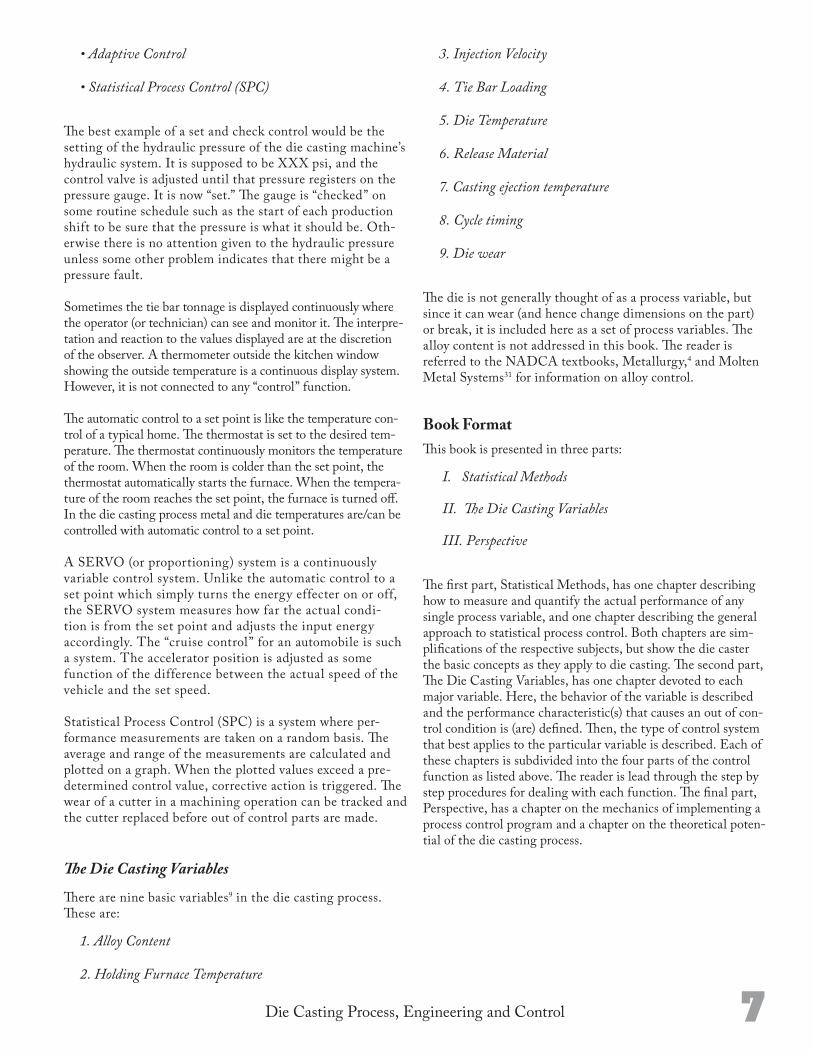
Control TheoryThere are four essential elements in any process control func­tion. These are:

1. Predetermined standard (ideal) condition

2. Measurement of actual condition

3. Comparison of actual to standard

4. Adjustment to process

Figure 1­1 illustrates these four elements. A typical process may have many inputs. Some may have a stronger influence on the output of the process than others. Sometimes one input has such a strong effect that it is the only one that needs to be controlled. The accelerator pedal in and automobile is such an example. There are many inputs that determine the exact speed that the vehicle is traveling at any instant. Some interpretation by the driver of the speed limit sign establishes the desired speed. The speedometer registers the actual speed. The driver then decides to adjust the speed based on the difference between the actual and desired speeds and adjusts the accelerator pedal accordingly. The driver does not concern himself with the exact position of the pedal. He pushes it down farther to go faster, and that action overcomes all other inputs.

Fig. 1­1. Processes are controlled by measuring the process var iables, comparing the actual condition to some desirable stand ard and making appropriate adjust-ments to the process. Tradi tionally, die casting has been controlled by a person performing all three functions.

Traditionally, the die casting machine operator performed the process control function. His effectiveness was limited by the insensitivity of the hu man senses, the need to guess the actual machine or process performance by observing the casting’s condition rather than measuring actual performance, and the

Introduction to Control Theory

6 Die Casting Process, Engineering and Control

is capable of the task. However, there is a chapter on the basic concepts of measuring process capabilities.

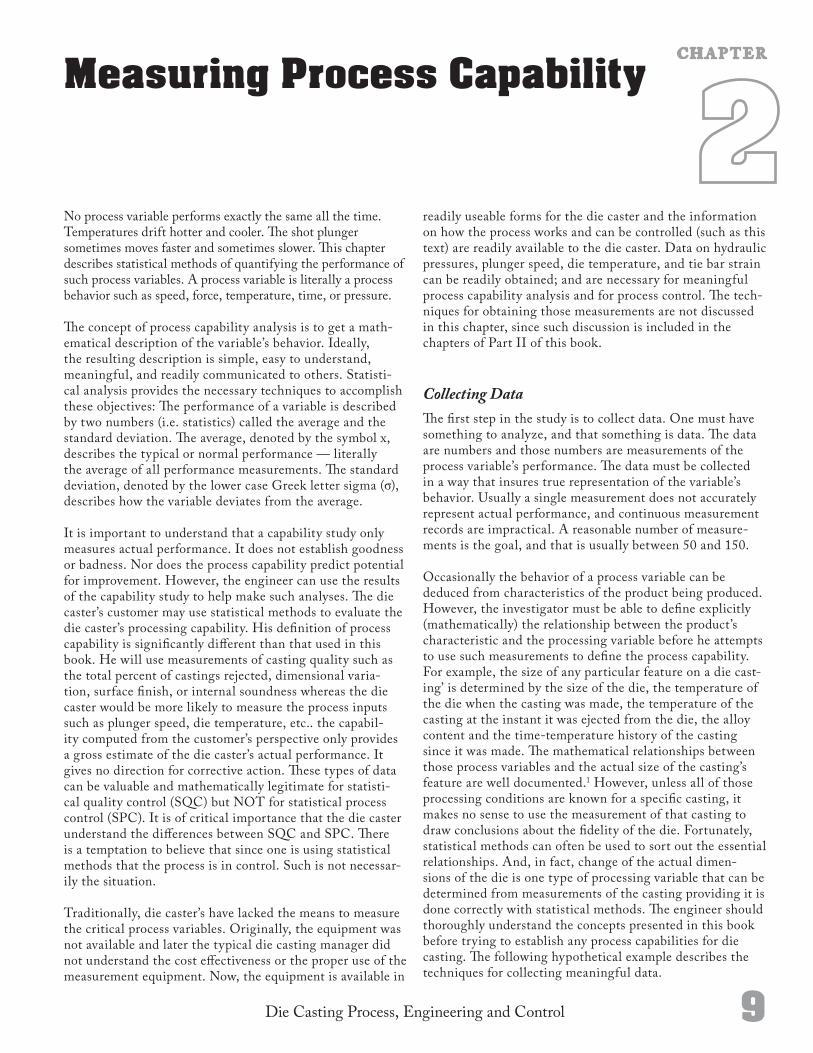
Process Control TheoryProcess control theory is that if one controls the inputs, the output of a process will be predictable and hence the output is not routinely measured to “control” the inputs. When all of the significant inputs are known and controlled, the output is indeed predictable. This concept is diagrammed in Figure 1­3.

Fig. 1­3. Process control theory is that by controlling all the inputs, the output will be predictable. The output, which in the case of die casting would be the cast-ing, is not measured and used in the control function.

It often turns out that each input to a manufacturing process has a feed­back control loop like that shown in Figure 1­1. There is some “process” that sets the input to the manufac­turing process.

Behavior of VariablesThe different types of performance characteristics that can cause a process to go out of control are:

1. Catastrophic event2. Continuous drift3. Cyclic drift 4. Threshold condition.

The breaking of a drill is an example of a catastrophic event. All parts prior to breakage are fine, but the parts after break­age have no hole. The process is no longer operating within the predetermined range. The process is “out of control.” If the cost of having parts without the hole is low, periodic inspection is adequate measurement of the actual processing condition. Once the process is discovered to be out of control (i.e. no holes), the condition is corrected (i.e. drill replaced), and all parts made since the previous inspection are repro­cessed. If the absence of the hole is very expensive, then every part must be checked to insure it has a hole before it leaves the operation. Small core pins in a die cavity can break caus­ing catastrophic event type conditions.

Processing variables that have continuous drift in one direc­tion are ideally suited for statistical process control (SPC) methods. For example, if wear of a cutting tool (or a surface in a die casting die) makes a di mension larger, successive parts will gradually get bigger. If an appropriate number of parts are checked for size at appro priate intervals (e.g. five parts each hour) an SPC average and range chart can be plotted to show graphically the proc ess drift. Then corrective action can be taken before the proc ess makes parts with dimensions outside the pre­established range. Wear of die cavity surfaces and dete­riorating hydrau lic components of the die casting machine can cause such continuously drifting situations.

More typical of die casting variables is cyclic drift. Die tem­perature is an example of cyclic drift. Over a period of several hours, the temperature at any one spot in the die will vary substantially. Sometimes hot, sometimes cold, and eve rywhere between. Periodic inspection and statistical process control techniques are not generally effective for controlling cyclic drift variables. By the time an out of control condition is found or predicted, the performance cycle may have re versed itself. Then any adjustment to the process will be wrong. Continuous control is required for these variables.

A threshold condition is when a cyclic or continuously drift­ing variable causes a catastrophic failure to some critical actual performance value. Often, the variation prior to the catastrophic event has little or no effect on the product being made. The temperature differential of the plunger and shot sleeve is a process variable with a threshold condition. As these temperatures change (cyclically) the plunger and bore change sizes. Within a range of sizes there is no impact on the castings being made. But at some point, the plunger will stick with dramatic results to the casting.

Control of the die casting process is difficult because it has variables exhibiting all four performance characteristics. It also has mutually compensating variables. For example, the appearance of the casting might get bad because the plunger is slow. The operator might correct the appearance by reduc­ing the flow of cooling water and therefore making the die hotter. Conceptualization is also difficult, because the process can appear quite different from different view points. The customer who forces his supplier of die castings to adopt some specific technique (such as statistical process control) because of a perceived situation could very well be doing the wrong thing. The process theory should be understood be fore corrective action is taken.

Control MethodsThere are several methods for controlling the input variables to a process. The most common are:

• Set and Check

• Continuous Display – Operator Monitor

• Automatic Control to Set Point

• SERVO Control

7Die Casting Process, Engineering and Control

• Adaptive Control

• Statistical Process Control (SPC)

The best example of a set and check control would be the setting of the hydraulic pressure of the die casting machine’s hydraulic system. It is supposed to be XXX psi, and the control valve is adjusted until that pressure registers on the pressure gauge. It is now “set.” The gauge is “checked” on some routine schedule such as the start of each production shift to be sure that the pressure is what it should be. Oth­erwise there is no attention given to the hydraulic pressure unless some other problem indicates that there might be a pressure fault.

Sometimes the tie bar tonnage is displayed continuously where the operator (or technician) can see and monitor it. The interpre­tation and reaction to the values displayed are at the discretion of the observer. A thermometer outside the kitchen window showing the outside temperature is a continuous display system. However, it is not connected to any “control” function.

The automatic control to a set point is like the temperature con­trol of a typical home. The thermostat is set to the desired tem­perature. The thermostat continuously monitors the temperature of the room. When the room is colder than the set point, the thermostat automatically starts the furnace. When the tempera­ture of the room reaches the set point, the furnace is turned off. In the die casting process metal and die temperatures are/can be controlled with automatic control to a set point.

A SERVO (or proportioning) system is a continuously variable control system. Unlike the automatic control to a set point which simply turns the energy effecter on or off, the SERVO system measures how far the actual condi­tion is from the set point and adjusts the input energy accordingly. The “cruise control” for an automobile is such a system. The accelerator position is adjusted as some function of the difference between the actual speed of the vehicle and the set speed.

Statistical Process Control (SPC) is a system where per­formance measurements are taken on a random basis. The average and range of the measurements are calculated and plotted on a graph. When the plotted values exceed a pre­determined control value, corrective action is triggered. The wear of a cutter in a machining operation can be tracked and the cutter replaced before out of control parts are made.

The Die Casting Variables

There are nine basic variables9 in the die casting process. These are:

1. Alloy Content

2. Holding Furnace Temperature

3. Injection Velocity

4. Tie Bar Loading

5. Die Temperature

6. Release Material

7. Casting ejection temperature

8. Cycle timing

9. Die wear

The die is not generally thought of as a process variable, but since it can wear (and hence change dimensions on the part) or break, it is included here as a set of process variables. The alloy content is not addressed in this book. The reader is referred to the NADCA textbooks, Metallurgy,4 and Molten Metal Systems31 for in formation on alloy control.

Book FormatThis book is presented in three parts:

I. Statistical Methods

II. The Die Casting Variables

III. Perspective

The first part, Statistical Methods, has one chapter describ ing how to measure and quantify the actual performance of any single process variable, and one chapter describing the general approach to statistical process control. Both chapters are sim­plifications of the respective subjects, but show the die caster the basic concepts as they apply to die casting. The second part, The Die Casting Variables, has one chapter de voted to each major variable. Here, the behavior of the varia ble is described and the performance characteristic(s) that causes an out of con­trol condition is (are) defined. Then, the type of control system that best applies to the particular variable is described. Each of these chapters is subdivided into the four parts of the control function as listed above. The reader is lead through the step by step procedures for dealing with each function. The final part, Perspective, has a chapter on the mechanics of imple menting a process control program and a chapter on the theo retical poten­tial of the die casting process.

Die Casting Process, Engineering and Control 9

No process variable performs exactly the same all the time. Temperatures drift hotter and cooler. The shot plunger sometimes moves faster and sometimes slower. This chapter describes statistical methods of quantifying the performance of such process variables. A process variable is literally a process behavior such as speed, force, temperature, time, or pressure.

The concept of process capability analysis is to get a math­ematical description of the variable’s behavior. Ideally, the resulting description is simple, easy to understand, meaning ful, and readily communicated to others. Statisti­cal analysis provides the necessary techniques to accomplish these objec tives: The performance of a variable is described by two numbers (i.e. statistics) called the average and the standard de viation. The average, denoted by the symbol x, describes the typical or normal performance — literally the average of all performance measurements. The standard deviation, de noted by the lower case Greek letter sigma (σ), describes how the variable deviates from the average.

It is important to understand that a capability study only measures actual performance. It does not establish goodness or badness. Nor does the process capability predict potential for improve ment. However, the engineer can use the results of the capa bility study to help make such analyses. The die caster’s customer may use statistical methods to evaluate the die caster’s processing capability. His definition of process capability is significantly different than that used in this book. He will use measurements of casting quality such as the total percent of castings rejected, dimensional varia­tion, surface finish, or internal soundness whereas the die caster would be more likely to measure the process inputs such as plunger speed, die temperature, etc.. the capabil­ity computed from the customer’s perspective only provides a gross estimate of the die caster’s actual performance. It gives no direction for corrective action. These types of data can be valuable and mathemati cally legitimate for statisti­cal quality control (SQC) but NOT for statistical process control (SPC). It is of critical impor tance that the die caster understand the differences between SQC and SPC. There is a temptation to believe that since one is using statistical methods that the process is in control. Such is not necessar­ily the situation.

Traditionally, die caster’s have lacked the means to mea sure the critical process variables. Originally, the equipment was not available and later the typical die casting manager did not understand the cost effectiveness or the proper use of the measurement equipment. Now, the equipment is availa ble in

Measuring Process CapabilityC H A P T E R

readily useable forms for the die caster and the information on how the process works and can be controlled (such as this text) are readily available to the die caster. Data on hy draulic pressures, plunger speed, die temperature, and tie bar strain can be readily obtained; and are necessary for meaningful process capability analysis and for process control. The tech­niques for obtaining those measurements are not discussed in this chapter, since such discussion is included in the chapters of Part II of this book.

Collecting DataThe first step in the study is to collect data. One must have something to analyze, and that something is data. The data are numbers and those numbers are measurements of the process variable’s performance. The data must be collected in a way that insures true representation of the variable’s be havior. Usually a single measurement does not accurately represent actual performance, and continuous measurement records are impractical. A reasonable number of measure­ments is the goal, and that is usually between 50 and 150.

Occasionally the behavior of a process variable can be deduced from characteristics of the product being produced. However, the investigator must be able to define explicitly (mathematically) the relationship between the product’s characteristic and the processing variable before he attempts to use such measurements to define the process capability. For example, the size of any particular feature on a die cast­ing’ is determined by the size of the die, the temperature of the die when the casting was made, the temperature of the casting at the instant it was ejected from the die, the alloy content and the time­temperature history of the casting since it was made. The mathematical relationships between those process variables and the actual size of the casting’s feature are well documented.1 However, unless all of those process ing conditions are known for a specific casting, it makes no sense to use the measurement of that casting to draw conclu sions about the fidelity of the die. Fortunately, statistical methods can often be used to sort out the essential relation ships. And, in fact, change of the actual dimen­sions of the die is one type of processing variable that can be determined from measurements of the casting providing it is done cor rectly with statistical methods. The engineer should thoroughly understand the concepts presented in this book before trying to establish any process capabilities for die casting. The following hypothetical example describes the tech niques for collecting meaningful data.

10 Die Casting Process, Engineering and Control

Reading Number Day Time of Day Value of

Reading °F1 1st 9:50 316

2 1st 11:20 352

3 1st 1:40 358

4 1st 3:30 386

5 1st 4:20 361

6 1st 6:10 374

7 1st 7:30 344

8 1st 8:40 337

9 1st 10:30 351

10 2nd 8:10 348

11 2nd 9:30 326

12 2nd 11:00 301

13 2nd 11:40 329

14 2nd 12:10 346

15 2nd 1:40 364

16 2nd 2:50 399

17 2nd 3:20 384

18 2nd 4:10 371

19 2nd 5:40 367

20 2nd 6:00 364

21 2nd 6:40 351

22 2nd 9:00 376

23 2nd 9:30 362

24 2nd 9:50 344

25 2nd 10:30 345

26 2nd 10:50 348

27 3rd 8:30 336

28 3rd 8:40 316

29 3rd 9:20 328

30 3rd 10:20 334

31 3rd 12:40 302

32 3rd 1:50 316

33 3rd 2:50 334

34 3rd 3:40 343

35 3rd 4:20 366

36 3rd 6:20 374

37 3rd 7:20 365

38 3rd 9:50 358

39 4th 8:10 351

40 4th 8:40 354

41 4th 11:10 344

42 4th 12:50 324

43 4th 2:00 318

44 4th 4:10 330

45 4th 5:10 336

46 4th 6:00 366

47 4th 7:20 381

48 4th 7:30 374

49 4th 9:30 387

50 4th 12:00 374

51 5th 10:00 354

52 5th 11:20 356

53 5th 1:20 358

54 5th 3:30 346

55 5th 3:40 336

56 5th 3:50 324

57 5th 6:00 316

58 5th 8:30 326

59 5th 8:50 344

60 5th 11:00 355

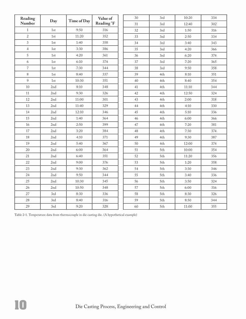
Table 2­1. Temperature data from thermocouple in die casting die. (A hypothetical example)

11Die Casting Process, Engineering and Control

In this example, it has been assumed that a thermocouple was installed midway between a waterline and the cavity sur face of a die casting die. Temperature readings were made from the thermocouple and recorded as shown in Table 2­1. The readings were made at random intervals during one week of continuous two shift operation. All readings were taken during normal operation. The machine was assumed to be operating on eight hour shifts with no break between shifts. Operator break and lunch periods were relieved so there was no break in the operation once the machine was started in the morning. No measurements were taken during the first hour each day. Temperatures were known to vary widely during that first hour because of die “warm up” and few saleable castings were made during that time. The time between measurements was selected randomly in ten minute increments from a minimum of ten minutes to a maximum of 150 minutes. It is important that measurements for statistical analysis be taken on a random basis. Random time intervals eliminate the chance of taking all measurements at the same point of a processing cycle. And, it is important that they only represent normal operat­ing conditions. Die warm up periods and times when some­thing is not working right (such as when the waterline was plugged so the die was being run slowly with excess die lube to “finish off the run”) must not be used to obtain process capability data. (Data from such abnormal conditions can be used to establish the degree to which such operating condi­tions hurt the process. But such data is only useful once the capability of normal conditions is quantified. Such studies deal with the risks associated with uncontrolled processes, and that is beyond the scope of this book.)

Graphical RepresentationsData as collected (i.e. Table 2­1) is difficult to understand and to grasp significant meanings from. Even though the sta tistics of average and standard deviation can be computed directly from the raw data, it is usually helpful to first depict the data pictorially. The frequency distribution and time plot are two types of graphs that are particularly helpful for under standing the nature of the variable being analyzed.

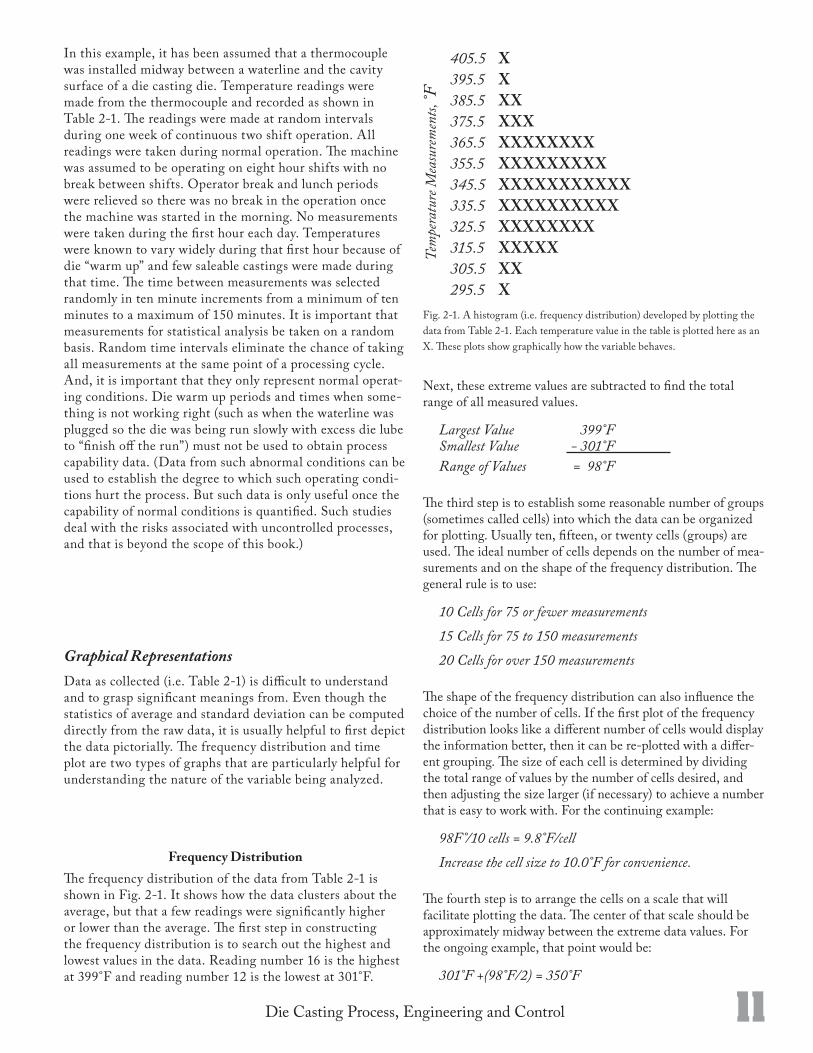
Frequency DistributionThe frequency distribution of the data from Table 2­1 is shown in Fig. 2­1. It shows how the data clusters about the average, but that a few readings were significantly higher or lower than the average. The first step in constructing the frequency distribution is to search out the highest and lowest values in the data. Read ing number 16 is the highest at 399°F and reading number 12 is the lowest at 301°F.

Tem

pera

ture

Mea

surem

ents,

°F

405.5 X395.5 X385.5 XX375.5 XXX365.5 XXXXXXXX355.5 XXXXXXXXX345.5 XXXXXXXXXXX335.5 XXXXXXXXXX325.5 XXXXXXXX315.5 XXXXX305.5 XX295.5 X

Fig. 2­1. A histogram (i.e. frequency distribution) developed by plotting the data from Table 2­1. Each temperature value in the table is plotted here as an X. These plots show graphically how the variable behaves.

Next, these extreme values are subtracted to find the total range of all measured values.

Largest Value 399°FSmallest Value - 301°FRange of Values = 98°F

The third step is to establish some reasonable number of groups (sometimes called cells) into which the data can be organized for plotting. Usually ten, fifteen, or twenty cells (groups) are used. The ideal number of cells depends on the number of mea­surements and on the shape of the frequency distribution. The general rule is to use:

10 Cells for 75 or fewer measurements 15 Cells for 75 to 150 measurements 20 Cells for over 150 measurements

The shape of the frequency distribution can also influence the choice of the number of cells. If the first plot of the fre quency distribution looks like a different number of cells would display the information better, then it can be re­plotted with a differ­ent grouping. The size of each cell is determined by dividing the total range of values by the num ber of cells desired, and then adjusting the size larger (if nec essary) to achieve a number that is easy to work with. For the continuing example:

98F°/10 cells = 9.8°F/cellIncrease the cell size to 10.0°F for convenience.

The fourth step is to arrange the cells on a scale that will facilitate plotting the data. The center of that scale should be approximately midway between the extreme data values. For the ongoing example, that point would be:

301°F +(98°F/2) = 350°F

12 Die Casting Process, Engineering and Control

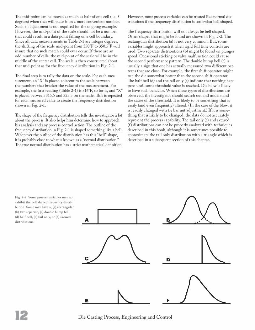
Fig. 2­2. Some process variables may not exhibit the bell shaped fre quency distri­bution. Some may have a, (a) rectangular, (b) two sep arate, (c) double hump bell, (d) half bell, (e) tail only, or (f ) skewed dis tributions.

The mid­point can be moved as much as half of one cell (i.e. 5 degrees) when that will place it on a more convenient num ber. Such an adjustment is not required for the ongoing exam ple. However, the mid­point of the scale should not be a num ber that could result in a data point falling on a cell boundary. Since all data measurements in Table 2­1 are integer degrees, the shifting of the scale mid­point from 350°F to 350.5°F will insure that no such match could ever occur. If there are an odd number of cells, the mid­point of the scale will be in the middle of the center cell. The scale is then constructed about that mid­point as for the frequency distribution in Fig. 2­1.

The final step is to tally the data on the scale. For each mea­surement, an “X” is placed adjacent to the scale between the numbers that bracket the value of the measurement. For example, the first reading (Table 2­1) is 316°F, so for it, and “X” is placed between 315.5 and 325.5 on the scale. This is repeated for each measured value to create the frequency dis tribution shown in Fig. 2­1.

The shape of the frequency distribution tells the investiga tor a lot about the process. It also helps him determine how to approach his analysis and any process control action. The outline of the frequency distribution in Fig. 2­1 is shaped something like a bell. Whenever the outline of the distribu tion has this “bell” shape, it is probably close to what is known as a “normal distribution.” The true normal distribution has a strict mathematical definition.

However, most process variables can be treated like normal dis­tributions if the fre quency distribution is somewhat bell shaped.

The frequency distribution will not always be bell shaped. Other shapes that might be found are shown in Fig. 2­2. The rectangular distribution (a) is not very common. But, some variables might approach it when rigid full time controls are used. Two separate distributions (b) might be found on plunger speed. Occasional sticking or valve malfunction could cause the second performance pattern. The double hump bell (c) is usually a sign that one has actually measured two different pat­terns that are close. For example, the first shift operator might run the die somewhat hotter than the second shift operator. The half bell (d) and the tail only (e) indicate that nothing hap­pens until some threshold value is reached. Die blow is likely to have such behavior. When these types of distributions are observed, the investigator should search out and understand the cause of the threshold. It is likely to be something that is easily (and even frequently) altered. (In the case of die blow, it is readily changed with tie bar nut adjustment.) If it is some­thing that is likely to be changed, the data do not accurately represent the process ca pability. The tail only (e) and skewed (f) distributions can not be properly analyzed with techniques described in this book, although it is sometimes possible to approximate the tail only distribution with a triangle which is described in a subsequent section of this chapter.

13Die Casting Process, Engineering and Control

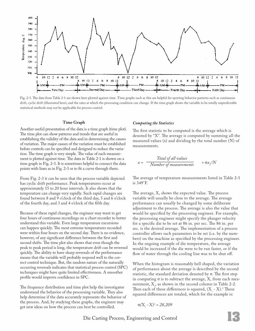
Fig. 2­3. The data from Table 2­1 are shown here plotted against time. Time graphs such as this are helpful for spotting behavior patterns such as continuous drift, cyclic drift (illustrated here), and the rates at which the processing condition can change. If the time graph shows the variable to be totally unpredictable statistical methods may not be applicable for process control.

Time GraphAnother useful presentation of the data is a time graph (time plot). The time plot can show patterns and trends that are useful in establishing the validity of the data and in deter mining the causes of variation. The major causes of the varia tion must be established before controls can be specified and designed to reduce the varia­tion. The time graph is very sim ple. The value of each measure­ment is plotted against time. The data in Table 2­1 is shown on a time graph in Fig. 2­3. It is sometimes helpful to connect the data points with lines as in Fig. 2­3 or to fit a curve through them.

From Fig. 2­3 it can be seen that the process variable de picted has cyclic drift performance. Peak temperatures occur at approximately 15 to 20 hour intervals. It also shows that the temperature can change very rapidly. Such rapid changes are found between 8 and 9 o’clock of the third day, 5 and 6 o’clock of the fourth day, and 3 and 4 o’clock of the fifth day.

Because of these rapid changes, the engineer may want to get four hours of continuous recordings on a chart recorder to better understand this variable. Even large temperature excursions can happen quickly. The most extreme temperatures re corded were within four hours on the second day. There is no evidence, however, of any significant difference between the first and second shifts. The time plot also shows that even though the peak to peak period is long, the temperature drift can be reversed quickly. The ability to have sharp reversals of the performance means that the variable will probably re spond well to the cor­rect control technique. But, the random nature of the naturally occurring reversals indicates that sta tistical process control (SPC) techniques might have quite limited effectiveness. A smoother profile would improve confidence in SPC.

The frequency distribution and time plot help the investi gator understand the behavior of the processing variable. They also help determine if the data accurately represents the behavior of the process. And, by studying these graphs, the engineer may get new ideas on how the process can best be controlled.

Computing the Statistics

The first statistic to be computed is the average which is denoted by “X”. The average is computed by summing all the measured values (x) and dividing by the total number (N) of measurements.

x = Total of all values

= σx1/N Number of measurements

The average of temperature measurements listed in Table 2­1 is 349°F.

The average, X, shows the expected value. The process vari able will usually be close to the average. The average per formance can usually be changed by some deliberate adjust ment to the process. The average is also the value that would be specified by the processing engineer. For example, the processing engi neer might specify the plunger velocity for a specific die to be set at 86 in. per sec. The 86 in. per sec. is the desired average. The implementation of a process controller allows such parameters to be set (i.e. by the num­bers) on the ma chine as specified by the processing engineer. In the ongoing exam ple of die temperature, the average would be increased if the die were to be run faster, or if the flow of water through the cooling line was to be shut off.

When the histogram is reasonably bell shaped, the varia tion of performance about the average is described by the second statistic, the standard deviation denoted by σ. The first step in computing σ is to subtract the average, X, from each mea­surement, Xi, as shown in the second column in Ta ble 2­2. Then each of these differences is squared, (Xi ­ X).2 These squared differences are totaled, which for the exam ple is:

σ(Xi ­ X)2 = 28,209

14 Die Casting Process, Engineering and Control

That total is then divided by the number of observations to obtain σ.2

σ2 = {Σ(Xi – X)2}/N

Which for the example is:σ2 = 28209/60 = 470.15

The standard deviation, σ, is therefore:σ = (470.15)0.5 = 21.8(approx.)

A truly normal distribution will have 99.73% of all data points within (+/­) three standard deviations of the average. And, a process is considered to be “in control” if it is operat­ing within that plus or minus 3σ range. So the normal operat­ing range of the die temperature in the example would be:

349°F ± 3(21.8F°) orfrom 284°F to 414°F

MeasurementX;

Difference X, — X

Difference Squared (X; - X)2

316 ­33 1089352 3 9358 9 81386 37 1367361 12 144374 25 625344 ­ 5 25337 ­12 144351 2 4348 ­ 1 1326 ­23 529301 ­48 2304329 ­20 400346 ­ 3 9364 15 225399 50 2500384 35 1225371 22 484367 18 324364 15 225351” 2 4376 27 729362 13 169344 ­ 5 25345 ­ 4 16348 ­ 1 1336 ­13 169316 ­33 1089328 ­21 441

334 ­15 225302 ­47 2209316 ­33 1089334 ­15 225343 ­ 6 36366 17 289374 25 625365 16 256358 9 81351 2 4354 5 25344 ­ 5 25324 ­25 625318 ­31 961330 ­19 361336 ­13 169366 17 289381 32 1024374 25 625387 38 1444374 25 625354 5 25356 7 49358 9 81346 ­ 3 9336 ­13 169324 ­25 625316 ­33 1089326 ­23 529344 ­ 5 25355 6 36

Table 2­2. The standard deviation, a, required that the difference between each value and the average be found (x, ­ x) and these differences be squared (x; ­x)2 and summed.

15Die Casting Process, Engineering and Control

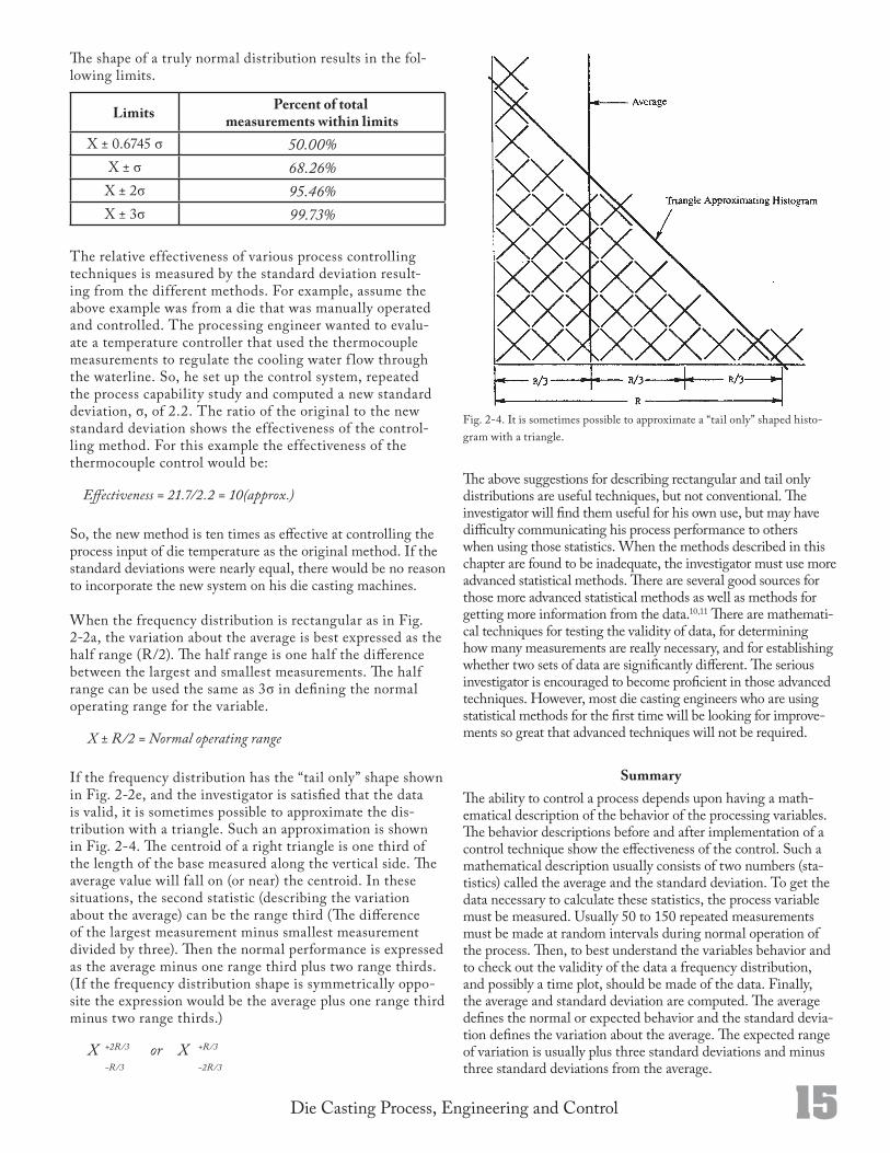
Fig. 2­4. It is sometimes possible to approximate a “tail only” shaped histo­gram with a triangle.

The above suggestions for describing rectangular and tail only distributions are useful techniques, but not conven tional. The investigator will find them useful for his own use, but may have difficulty communicating his process perform ance to others when using those statistics. When the methods described in this chapter are found to be inadequate, the in vestigator must use more advanced statistical methods. There are several good sources for those more advanced sta tistical methods as well as methods for getting more informa tion from the data.10,11 There are mathemati­cal techniques for testing the validity of data, for determining how many mea surements are really necessary, and for establishing whether two sets of data are significantly different. The serious inves tigator is encouraged to become proficient in those advanced techniques. However, most die casting engineers who are using statistical methods for the first time will be looking for improve­ments so great that advanced techniques will not be required.

SummaryThe ability to control a process depends upon having a math­ematical description of the behavior of the processing variables. The behavior descriptions before and after imple mentation of a control technique show the effectiveness of the control. Such a mathematical description usually consists of two numbers (sta­tistics) called the average and the stand ard deviation. To get the data necessary to calculate these statistics, the process variable must be measured. Usually 50 to 150 repeated measurements must be made at random inter vals during normal operation of the process. Then, to best understand the variables behavior and to check out the valid ity of the data a frequency distribution, and possibly a time plot, should be made of the data. Finally, the average and standard deviation are computed. The average defines the normal or expected behavior and the standard devia­tion de fines the variation about the average. The expected range of variation is usually plus three standard deviations and minus three standard deviations from the average.

The shape of a truly normal distribution results in the fol­lowing limits.

Limits Percent of total measurements within limits

X ± 0.6745 σ 50.00%X ± σ 68.26%

X ± 2σ 95.46%X ± 3σ 99.73%

The relative effectiveness of various process controlling techniques is measured by the standard deviation result­ing from the different methods. For example, assume the above example was from a die that was manually operated and con trolled. The processing engineer wanted to evalu­ate a tem perature controller that used the thermocouple measurements to regulate the cooling water f low through the waterline. So, he set up the control system, repeated the process capability study and computed a new standard deviation, σ, of 2.2. The ratio of the original to the new standard deviation shows the effectiveness of the control­ling method. For this example the effectiveness of the thermocouple control would be:

Effectiveness = 21.7/2.2 = 10(approx.)

So, the new method is ten times as effective at controlling the process input of die temperature as the original method. If the standard deviations were nearly equal, there would be no reason to incorporate the new system on his die casting machines.

When the frequency distribution is rectangular as in Fig. 2­2a, the variation about the average is best expressed as the half range (R/2). The half range is one half the difference between the largest and smallest measurements. The half range can be used the same as 3σ in defining the normal operating range for the variable.

X ± R/2 = Normal operating range

If the frequency distribution has the “tail only” shape shown in Fig. 2­2e, and the investigator is satisfied that the data is valid, it is sometimes possible to approximate the dis­tribution with a triangle. Such an approximation is shown in Fig. 2­4. The centroid of a right triangle is one third of the length of the base measured along the vertical side. The aver age value will fall on (or near) the centroid. In these situa tions, the second statistic (describing the variation about the average) can be the range third (The difference of the largest measurement minus smallest measurement divided by three). Then the normal performance is expressed as the av erage minus one range third plus two range thirds. (If the frequency distribution shape is symmetrically oppo­site the ex pression would be the average plus one range third minus two range thirds.)

X +2R/3 or X +R/3

-R/3 -2R/3

Die Casting Process, Engineering and Control 17

Statistical methods can be used to insure that a process is performing within its capability, predict that it is on the verge of behavior that is outside its normal capability or that it is actually operating outside its normal capability. Because of the behavior characteristics of most process variables in die cast­ing, statistical process control (SPC) is not usually an effective primary control method. Continuous control instrumentation is usually required. However, SPC is a very good technique for some variables, and is invaluable for verification that the primary control is working. Hard copies of such verification can be supplied to the customer as certification.

The first step in any SPC program is a good “process capabil­ity” study as described in Chapter 2. It makes no sense to try to keep something operating within its normal operating range if nothing is known about its performance behavior. Tradi­tionally, die casters have had only the most general notion of the actual performance of the variables. The process capabil­ity study used as a basis for the SPC program must show the capability of the process as it will perform for making the subject casting. The SPC program will not automatically cause better performance. It will only help the die caster insure that the process will not perform worse. Any improvement must be achieved through some physical change to the equipment, operating procedure and/or control instrumentation. Such changes will change the fundamental behavior of the process and a new process capability study will be required to measure the new performance.

The second step is to design the SPC program for the spe­cific process variable for the subject casting. The design of the program is the primary subject of this chapter. The program must define clearly the measurement method to be used, the inspection procedure and the inspection schedule. Then the charting technique must be designed and the calculations (with worksheets) specified. Finally, the program must have clearly defined decision criteria and specific corrective actions to be taken for specific situations.

The third step is to implement the program. Implementa­tion is a management, not an engineering or quality con­trol function. People must be assigned tasks and be held responsible for performing them. Also, budgets must be established. SPC programs are not free. And, if one tries to “bootleg” it through, other priorities will insure failure. (Sometimes test cases to prove the value of the program can be bootlegged, but that is the extent of it.) Finally, there is training. Everyone involved with, or exposed to, the

Statistical Process ControlC H A P T E R

program must be trained. It is obvious that those taking measurements, doing calculations and plotting charts must be properly trained. But, it is equally important that the production workers and managers also know what is being done, and why. Statistical process control cannot be accom­plished if management thinks it is something that “does not involve” or “must be hidden from” the machine operators. To be successful, the operators must take an active part in the process. It is the operating personnel who must react immediately to any out of control situation identified by the control process. It is the operating people for whom the control charts are created. For anyone else, the control chart is only interesting. It is also important that the management and marketing personnel understand the program. As stated in the previous paragraph, this chapter concentrates on the technical aspects of design and execution of an SPC pro­gram, not the management aspects. However, these imple­mentation considerations are critical to the success of the program and are therefore mentioned here.

The final step in a successful SPC program is continuing com­munication. It is not enough to collect and analyze measure­ments and plot charts. Even when the charted information actually results in action that causes consistent manufacture of high quality castings, it is not enough. Frequent communica­tions to management, marketing, engineering, the production operators and the customers are necessary to maintain the momentum of the program. Little things like the following memo are very important:

“On Tuesday, July 30, 2006, the SPC chart (attached) for machine number 6 showed that die temperature could be going out of control. The jobsetter, Joe Smith, took immediate action and discovered and immediately corrected a plugged waterline hose. As a result, no sub-quality castings were made. Another example of our SPC program at work,”

Such communications should go to everyone.”

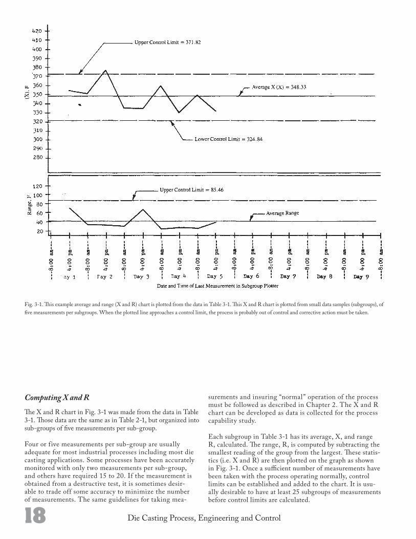
Average (X) and Range (R) ChartsThe basic tool for SPC is the average and range chart, com­monly referred to as the “X and R charts” (pronounced “X and R”). The X and R chart is a time plot of the averages, X, and ranges, R, of small groups (i.e. subgroups) of mea­surements taken at intervals (usually random intervals). An example chart is shown in Fig. 3­1.

18 Die Casting Process, Engineering and Control

Computing X and R

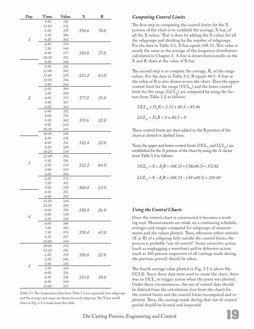
The X and R chart in Fig. 3­1 was made from the data in Table 3­1. Those data are the same as in Table 2­1, but organized into sub­groups of five measurements per sub­group.

Four or f ive measurements per sub­group are usually adequate for most industrial processes including most die casting applications. Some processes have been accurately monitored with only two measurements per sub­group, and others have required 15 to 20. If the measurement is obtained from a destructive test, it is sometimes desir­able to trade off some accuracy to minimize the number of measurements. The same guidelines for taking mea­

surements and insuring “normal” operation of the process must be followed as described in Chapter 2. The X and R chart can be developed as data is collected for the process capability study.

Each subgroup in Table 3­1 has its average, X, and range R, calculated. The range, R, is computed by subtracting the smallest reading of the group from the largest. These statis­tics (i.e. X and R) are then plotted on the graph as shown in Fig. 3­1. Once a sufficient number of measurements have been taken with the process operating normally, control limits can be established and added to the chart. It is usu­ally desirable to have at least 25 subgroups of measurements before control limits are calculated.

Fig. 3­1. This example average and range (X and R) chart is plotted from the data in Table 3­1. This X and R chart is plotted from small data samples (subgroups), of five measurements per subgroups. When the plotted line approaches a control limit, the process is probably out of control and corrective action must be taken.

19Die Casting Process, Engineering and Control

Day Time Value X R

1

9:50 316

354.6 70.011:20 352 1:40 358 3:30 386 4:20 361 6:10 374

350.8 37.0 7:30 344 8:40 33710:30 351

2

8:10 348 9:30 326

333.2 63.011:00 30111:40 32912:10 346 1:40 364 2:50 399

377.0 35.0 3:20 384 4:10 371 5:40 367 6:00 364 6:40 351

355.6 32.0 9:00 376 9:30 362 9:50 34410:30 34510:50 348

332.4 32.0

3

8:30 336 8:40 316 9:20 32810:20 33412:40 302

332.2 64.0 1:50 316 2:50 334 3:40 343 4:20 366 6:20 374

360.4 23.0 7:20 365 9:50 358

4

8:10 351 8:40 35411:10 344

330.4 26.012:50 324 2:00 318 4:10 330 5:10 336 6:00 366

370.4 43.0 7:20 381 7:30 374 9:30 38712:00 344

5

10:00 354

350.0 22.011:20 356 1:20 358 3:30 346 3:40 336 3:50 324

333.0 39.0 6:00 316 8:30 326 8:50 34411:00 355

Table 3­1. The temperature data from Table 2­1 are organized into subgroups and the average and range are shown for each subgroup. The X­bar and R chart in Fig. 3­1 is made from this table.

Computing Control LimitsThe first step in computing the control limits for the X portion of the chart is to establish the average, X­bar, of all the X values. That is done by adding the X values for all the subgroups and dividing by the number of subgroups. For the data in Table 3­1, X­bar equals 348.33. This value is nearly the same as the average of the frequency distribution calculated in Chapter 2. A line is drawn horizontally on the X and R chart at the value of X­bar.

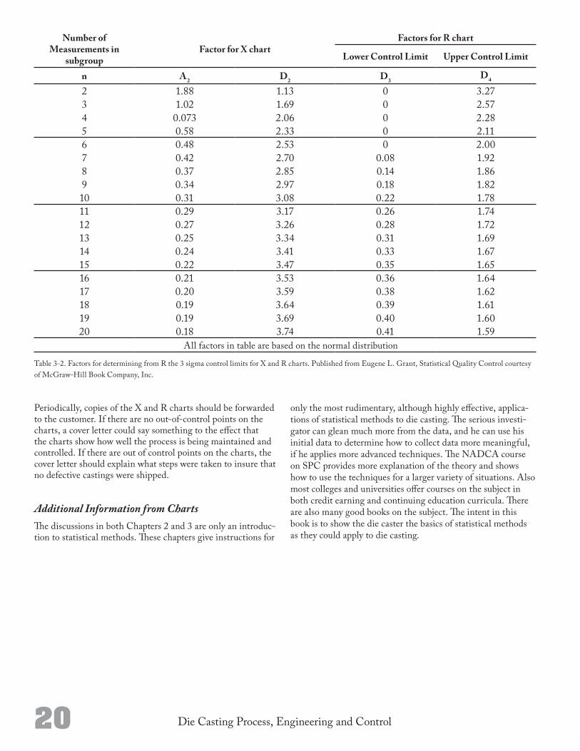
The second step is to compute the average, R, of the range values. For the data in Table 3­1, R equals 40.5. A line at the value of R is also drawn across the chart. Then the upper control limit for the range (UCLR) and the lower control limit for the range (LCLR) are computed by using the fac­tors from Table 3­2 as follows:

UCLR = D4R = 2.11 x 40.5 = 85.46

LCLR = D3R = 0 x 40.5 = 0

These control limits are then added to the R portion of the chart as dotted or dashed lines.

Next, the upper and lower control limits (UCLX and LCLX) are established for the X portion of the chart by using the A: factor from Table 3­2 as follows:

UCLX = X + A2R = 348.33 + (.58x40.5) = 371.82

LCLX = X - A2R = 348.33 - (.58 x40.5) = 324.84

Using the Control ChartsOnce the control chart is constructed it becomes a work­ing tool. Measurements are made on a continuing schedule, averages and ranges computed for subgroups of measure­ments and the values plotted. Then, whenever either statistic (X or R) of a subgroup falls outside the control limits, the process is probably “out of control”. Some corrective action (such as unplugging a waterline) and/or defensive action (such as 100 percent inspection of all castings made during the previous period) should be taken.

The fourth average value plotted in Fig. 3­1 is above the UCLX. Since those data were used to create the chart, there was no UCL, to trigger action when the point was plotted. Under these circumstances, the out of control data should be deleted from the calculations (not from the chart) for the control limits and the control limits recomputed and re­plotted. Then, the castings made during that out­of­control period should be located and inspected.

20 Die Casting Process, Engineering and Control

Number of Measurements in

subgroupFactor for X chart

Factors for R chart

Lower Control Limit Upper Control Limit

n A2 D2 D3D4

2 1.88 1.13 0 3.273 1.02 1.69 0 2.574 0.073 2.06 0 2.285 0.58 2.33 0 2.116 0.48 2.53 0 2.007 0.42 2.70 0.08 1.928 0.37 2.85 0.14 1.869 0.34 2.97 0.18 1.8210 0.31 3.08 0.22 1.7811 0.29 3.17 0.26 1.7412 0.27 3.26 0.28 1.7213 0.25 3.34 0.31 1.6914 0.24 3.41 0.33 1.6715 0.22 3.47 0.35 1.6516 0.21 3.53 0.36 1.6417 0.20 3.59 0.38 1.6218 0.19 3.64 0.39 1.6119 0.19 3.69 0.40 1.6020 0.18 3.74 0.41 1.59

All factors in table are based on the normal distribution

Table 3­2. Factors for determining from R the 3 sigma control limits for X and R charts. Published from Eugene L. Grant, Statistical Quality Control courtesy of McGraw­Hill Book Company, Inc.

Periodically, copies of the X and R charts should be forwarded to the customer. If there are no out­of­control points on the charts, a cover letter could say something to the effect that the charts show how well the process is being maintained and controlled. If there are out of control points on the charts, the cover letter should explain what steps were taken to insure that no defective castings were shipped.

Additional Information from ChartsThe discussions in both Chapters 2 and 3 are only an introduc­tion to statistical methods. These chapters give instructions for

only the most rudimentary, although highly effective, applica­tions of statistical methods to die casting. The serious investi­gator can glean much more from the data, and he can use his initial data to determine how to collect data more meaningful, if he applies more advanced techniques. The NADCA course on SPC provides more explanation of the theory and shows how to use the techniques for a larger variety of situations. Also most colleges and universities offer courses on the subject in both credit earning and continuing education curricula. There are also many good books on the subject. The intent in this book is to show the die caster the basics of statistical methods as they could apply to die casting.

Die Casting Process, Engineering and Control 22

Except for the alloying constituents (which are beyond the scope of this book), the temperature of the molten metal in the holding furnace is the first process variable that will influence the making of a die casting. And, it was probably the first variable to have had continuous feed back controls applied. Such controls must now be considered traditional practice in this application. The questions for today’s die caster are not if he needs metal temperature controls; but rather, how should his control system be configured to achieve the desired results. A second question could be: are the existing controls actually doing what one thinks they are doing? And finally, at what temperature should the molten metal be held for any specific casting.

Determining the Required PerformanceThe casting to be made determines the temperature at which the molten metal should be in the holding furnace. There can be some trade off between die temperature, cavity filling time and the temperature of the molten metal. Also, some alloys will experience excessive oxidation (e.g. dross) or other alloy degradation if held at too high a temperature, and some develop sludge if held at too low a temperature. The holding

Holding Furnace Temperature

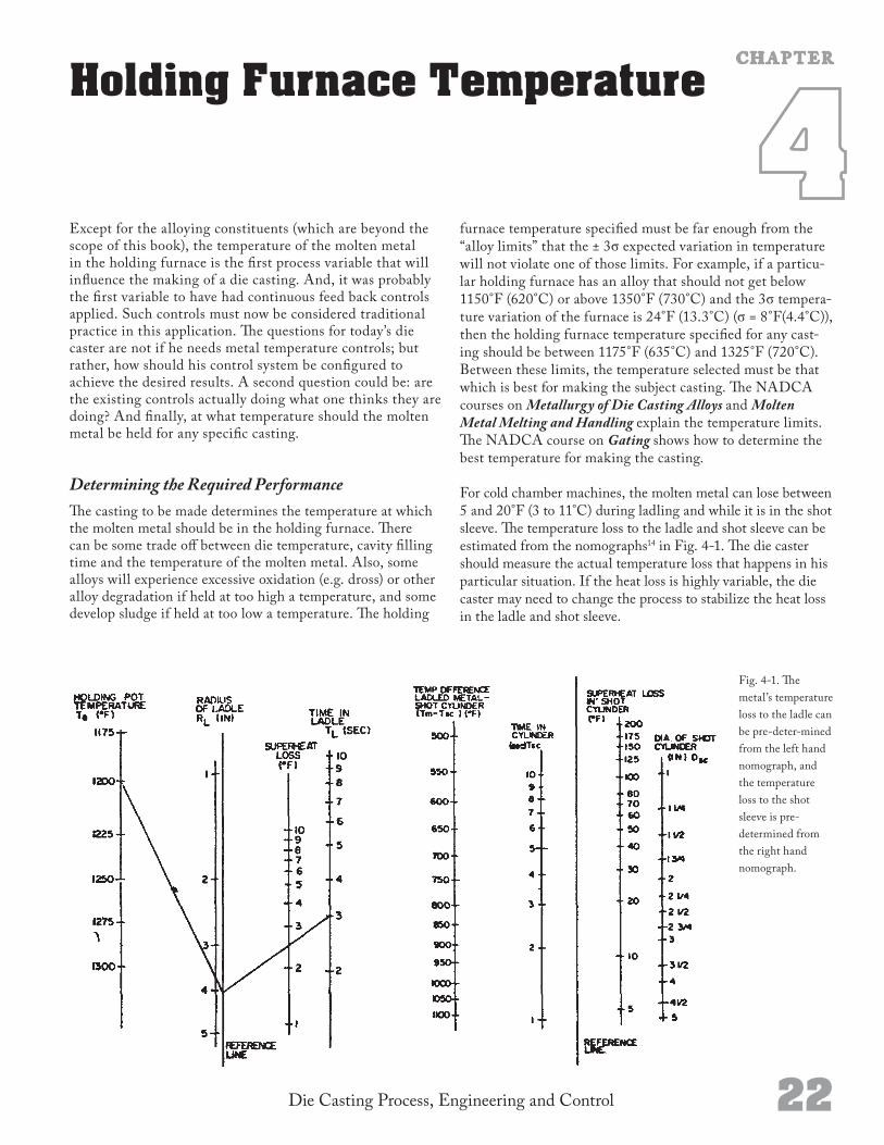
Fig. 4­1. The metal’s temperature loss to the ladle can be pre­deter­mined from the left hand nomograph, and the temperature loss to the shot sleeve is pre­determined from the right hand nomograph.

C H A P T E R

furnace temperature specified must be far enough from the “alloy limits” that the ± 3σ expected variation in temperature will not violate one of those limits. For example, if a particu­lar holding furnace has an alloy that should not get below 1150°F (620°C) or above 1350°F (730°C) and the 3σ tempera­ture variation of the furnace is 24°F (13.3°C) (σ = 8°F(4.4°C)), then the holding furnace temperature specified for any cast­ing should be between 1175°F (635°C) and 1325°F (720°C). Between these limits, the temperature selected must be that which is best for making the subject casting. The NADCA courses on Metallurgy of Die Casting Alloys and Molten Metal Melting and Handling explain the temperature limits. The NADCA course on Gating shows how to determine the best temperature for making the casting.

For cold chamber machines, the molten metal can lose between 5 and 20°F (3 to 11°C) during ladling and while it is in the shot sleeve. The temperature loss to the ladle and shot sleeve can be estimated from the nomographs14 in Fig. 4­1. The die caster should measure the actual temperature loss that happens in his particular situation. If the heat loss is highly variable, the die caster may need to change the process to stabilize the heat loss in the ladle and shot sleeve.

23 Die Casting Process, Engineering and Control

The next consideration is the effect of the metal temperature variation (± 24°F (13.9°C) in the above example) on the cast­ings to be made. Metal temperature can affect the surface finish and density of the casting. The process capability must be made available to the die and process engineer(s) so that it can be taken into account as the die gating system and the process set points are being calculated. The calculated die temperature and the plunger speeds could be effected by the metal temperature variation.

Changes in the holding furnace temperature can also cause variations in the castings dimensions’. Short term changes in the molten metal temperature will have a direct effect on the casting’s temperature at ejection if all other conditions are constant. If the holding furnace temperature increases 10°F (5.6°C), the castings will be about 10°F (5.6°C) hotter when ejected. The final size of the casting is determined by how much it shrinks after it is released from the die cavity. If the ejection temperature of consecutive aluminum castings was to change 40°F (22. 2°C), a 10 inch (254 mm) feature on the castings would change about 0.005 inch (0.127mm). The significance of the expected variation in percent solids or dimensions must be determined by the processing engineer. If the variation will be intolerable, modification or replace­ment of the holding furnace will be necessary.

Measuring and Controlling Actual PerformanceOnce the processing engineer has established the required holding furnace temperature and the acceptable variation from that temperature, the actual temperatures must be measured. A ceramic sheathed thermocouple15 is inserted (permanently) into the melt to make the temperature mea­surements. The thermocouple is connected to an indicating controller that displays the actual temperature and regulates the heat source. The furnace manufacturers can usually supply a furnace and control system to meet any situation provided the situation is clearly specified.

Existing furnaces may not have the same performance characteristics as new furnaces. Some furnaces, may not be properly sized for the job. The reader is referred to Chap­ter 2 for information on how to measure and quantify the furnace performance capability. When a capability study is made, the melt temperature should be measured in several places within the furnace. These places are: where the metal is ladled from the furnace, near the permanent thermo­couple, in each corner (or in three or four places around the perimeter if the furnace is round), and these measurements should be repeated near the top, near the center, and near the bottom.

Additional Control ActionsWhen temperature measurements from different regions of the furnace are significantly different, it may be necessary

to add circulation to the melt. Electric induction furnaces create a circulation, but electric resistance and gas fired furnaces do not. Sometimes a simple paddle submerged into the melt and rotated by an external motor will suffice. Some prefer molten metal pumps.9 When the process capability study is made, it could show that the location of the per­manent thermocouple is at a different temperature than the area where the metal is ladled from. Circulation can solve that problem, but it might also be appropriate to relocate the permanent thermocouple, or to offset the temperature set point by the amount of the difference.

One problem that could arise is that a furnace may never achieve the specified (i.e. set point) temperature. This phenom­enon is fairly common where a single furnace is used for both melting and holding and the furnace is overloaded. In these instances the furnace is simply too small. It must be replaced or the throughput reduced. Sometimes, however, the condition indicates improper burner adjustment or that covers and other insulation should be added. It could also indicate that molten metal being delivered to the furnace is too cold.

Alloy

Solid metal addedfor each

1000 lb -°F of temperature reduction

desired, lbs.

for each 1000 kg -°C

of temperature reduction desired, kg.

Mg 0.678 0.122Al 0.568 0.102Cu 0.407 0.073Fe 0.278 0.050Zn

(3, 5, 7)0.911 0.164

ZA (12, 27)

0.715 0.129

Pb 1.191 0.214

Table 4­1. When metal charged into a holding furnace is hotter than the desired temperature of the furnace, the extra heat can be compensated by adding the correct amount of solid metal (room temperature).

It is common for the delivery of molten metal to a holding furnace to be hotter or colder than the desired temperature of the holding furnace. When such charging of the furnace drives the temperature unacceptably low it is not a control problem as much as a capacity problem. But, more frequent charging with smaller amounts will help as will having the delivered metal hotter. When the charging drives the temperature too high, the charging can be done more fre­quently, or the temperature of the delivered metal lowered. Another alternative is to add some bars of alloy or trimmed runners and biscuits to the holding furnace each time it is

24Die Casting Process, Engineering and Control

refilled. Table 4­1 shows how many pounds of room tem­perature metal must be added for each 1000 pound­degrees of excess heat that is added with each refill of the furnace. The pound­degrees are found by multiplying the pounds of metal added to the furnace by the difference in temperature between the holding furnace and the metal being added. For example, suppose a holding furnace of aluminum should be at 1225°F (663°C), but it is periodically charged with 150 lbs. (68 kg) of molten alloy at 1275°F (691°C). The tempera­ture difference is:

Charge Temperature 1275°F (691°C)

Furnace Temperature 1225°F (663°C)

Temp. Difference 50°F ( 28°C)

Each charging is 150 Lbs. (68 kg), so:

Temp. diff. x Charge weight = 50°F x 150 Lbs. (28°C) (68kg) = 7500 Lb.-°F (1900 kg-°C)

From Table 4-1, one finds that 0.568 Lbs. (0.258 kg) of alloy must be added for each 1,000 Lb.-degs. (252 kg-°C), so:

{7500Lbs.-°F (1900kg.-°C) x 0.568 Lbs. (0.257 kg.)}/{1000 Lb.-°F (252kg.-°C)}= 4.26 Lbs. (1.93 kg.) of solid metal to be added

Such additions can be made as a regular procedure and can constitute a legitimate temperature control practice.

Die Casting Process, Engineering and Control 26

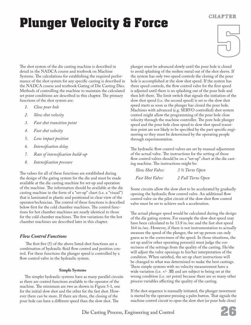
The shot system of the die casting machine is described in detail in the NADCA course and textbook on Machine Systems. The calculations for establishing the required perfor­mance of the shot system for any specific casting is described in the NADCA course and textbook Gating of Die Casting Dies. Methods of controlling the machine to maintain the calculated set point conditions are described in this chapter. The primary functions of the shot system are:

1. Close pour hole

2. Slow shot velocity

3. Fast shot transition point

4. Fast shot velocity

5. Low impact position

6. Intensification delay

7. Rate of intensification build-up

8. Intensification pressure

The values for all of these functions are established during the design of the gating system for the die and must be made available at the die casting machine for set­up and operation of the machine. The information should be available at the die casting machine in the form of a “set­up” chart (i.e. a “visual”) that is laminated in plastic and positioned in clear view of the operator/technician. The control of these functions is described below first for the cold chamber machines. The control func­tions for hot chamber machines are nearly identical to those for the cold chamber machines. The few variations for the hot chamber machines are described later in this chapter.

Flow Control Functions The first five (5) of the above listed shot functions are a

combination of hydraulic fluid flow control and position con­trol. For these functions the plunger speed is controlled by a flow control valve in the hydraulic system.

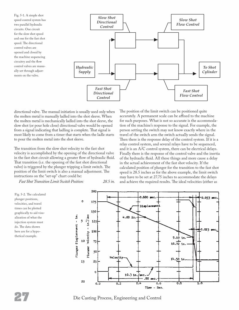
Simple SystemsThe simpler hydraulic systems have as many parallel circuits

as there are control functions available to the operator of the machine. The minimum are two as shown in Figure 5­1, one for the initial slow shot and the other for the fast shot. How­ever there can be more. If there are three, the closing of the pour hole can have a different speed than the slow shot. The

Plunger Velocity & ForceC H A P T E R

plunger must be advanced slowly until the pour hole is closed to avoid splashing of the molten metal out of the shot sleeve. If the system has only two speed controls the closing of the pour hole is accomplished at the slow shot speed. If the system has three speed controls, the flow control valve for the first speed is adjusted until there is no splashing out of the pour hole and then left there. The limit switch that signals the initiation of the slow shot speed (i.e. the second speed) is set so the slow shot speed starts as soon as the plunger has closed the pour hole. Machines with advanced (e.g. SERVO controlled) shot system control might allow the programming of the pour hole close velocity through the machine controller. The pore hole plunger speed and the pour hole close speed to slow shot speed transi­tion point are not likely to be specified by the part specific engi­neering so they must be determined by the operating people through experimentation.

The hydraulic flow control valves are set by manual adjustment of the actual valve. The instructions for the setting of those flow control valves should be on a “set­up” chart at the die cast­ing machine. The instructions might be:

Slow Shot Valve: 3 ½ Turns Open

Fast Shot Valve: 2 Full Turns Open

Some circuits allow the slow shot to be accelerated by gradually opening the hydraulic flow control valve. An additional flow control valve on the pilot circuit of the slow shot flow control valve must be set to achieve such a acceleration.

The actual plunger speed would be calculated during the design of the die gating system. For example the slow shot speed may have been calculated to be 13.8 in./sec and the fast shot speed 164 in./sec. However, if there is not instrumentation to actually measure the speed of the plunger, the set up person can only guess as to the correctness of the speed. In those situations, the set up and/or other operating person(s) must judge the cor­rectness of the settings from the quality of the casting. He/she will adjust the valve openings to his/her interpretation of the condition. When satisfied, the set up chart instructions will be changed to what was determined to make the best castings. These simple systems with no velocity measurement have a wide variation (i.e. +/­ 3σ) and are subject to being set at the wrong condition (i.e. set point) because there are so many other process variables affecting the quality of the casting.

If the shot sequence is manually initiated, the plunger movement is started by the operator pressing a palm button. That signals the machine control circuit to open the slow shot (or pour hole close)

27 Die Casting Process, Engineering and Control

directional valve. The manual initiation is usually used only when the molten metal is manually ladled into the shot sleeve. When the molten metal is mechanically ladled into the shot sleeve, the slow shot (or pour hole close) directional valve would be opened from a signal indicating that ladling is complete. That signal is most likely to come from a timer that starts when the ladle starts to pour the molten metal into the shot sleeve.

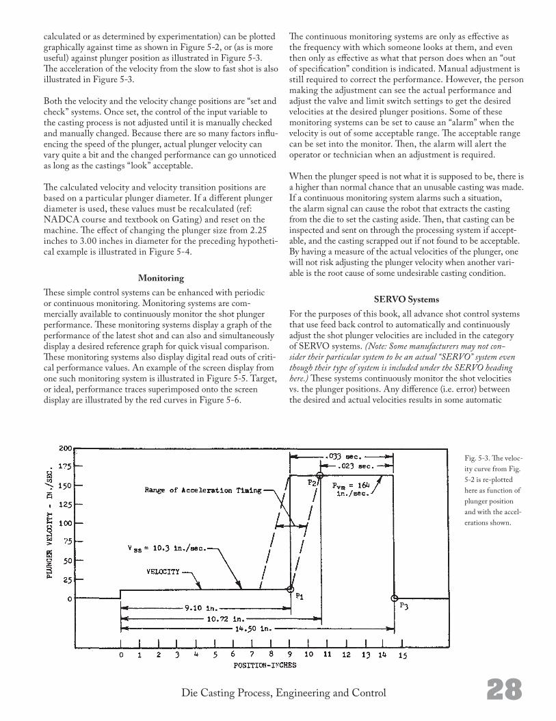
The transition from the slow shot velocity to the fast shot velocity is accomplished by the opening of the directional valve in the fast shot circuit allowing a greater flow of hydraulic fluid. That transition (i.e. the opening of the fast shot directional valve) is triggered by the plunger tripping a limit switch. The position of the limit switch is also a manual adjustment. The instructions on the “set­up” chart could be:

Fast Shot Transition Limit Switch Position: 28.5 in.

The position of the limit switch can be positioned quite accurately. A permanent scale can be affixed to the machine for such purposes. What is not so accurate is the accommoda­tion of the machine’s response to the signal. For example, the person setting the switch may not know exactly where in the travel of the switch arm the switch actually sends the signal. Then there is the response delay of the control system. If it is a relay control system, and several relays have to be sequenced, and it is an A/C control system, there can be electrical delays. Finally there is the response of the control valve and the inertia of the hydraulic fluid. All these things and more cause a delay in the actual achievement of the fast shot velocity. If the calculated position of plunger for the transition to the fast shot speed is 28.5 inches as for the above example, the limit switch may have to be set at 27.75 inches to accommodate the delays and achieve the required results. The ideal velocities (either as

Fig. 5­1. A simple shot speed control system has two parallel hydraulic circuits. One circuit for the slow shot speed and one for the fast shot speed. The directional control valves are opened and closed by the machine sequencing circuitry and the flow control valves are manu­ally set through adjust­ments on the valve.

Fig. 5­2. The calculated plunger positions, velocities, and travel times can be plotted graphically to aid visu­alization of what the injection system must do. The data shown here are for a hypo­thetical example.

28Die Casting Process, Engineering and Control

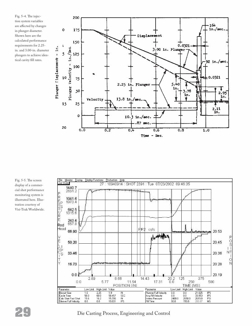
calculated or as determined by experimentation) can be plotted graphically against time as shown in Figure 5­2, or (as is more useful) against plunger position as illustrated in Figure 5­3. The acceleration of the velocity from the slow to fast shot is also illustrated in Figure 5­3.

Both the velocity and the velocity change positions are “set and check” systems. Once set, the control of the input variable to the casting process is not adjusted until it is manually checked and manually changed. Because there are so many factors influ­encing the speed of the plunger, actual plunger velocity can vary quite a bit and the changed performance can go unnoticed as long as the castings “look” acceptable.

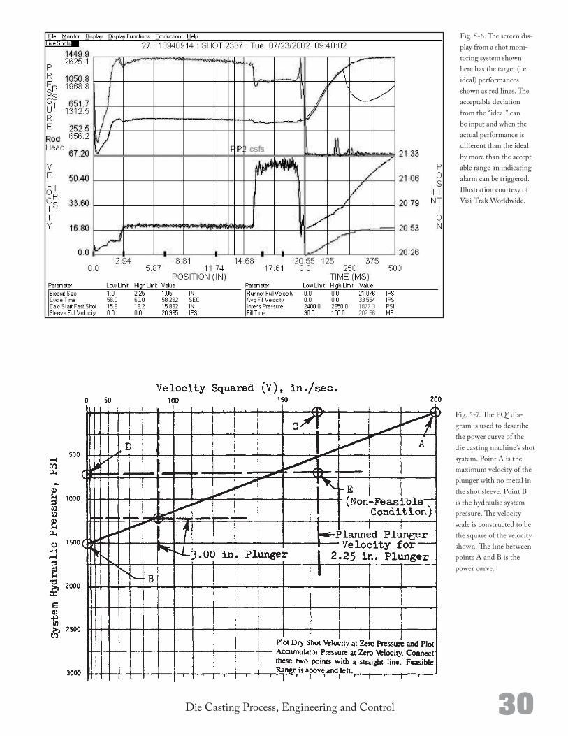
The calculated velocity and velocity transition positions are based on a particular plunger diameter. If a different plunger diameter is used, these values must be recalculated (ref: NADCA course and textbook on Gating) and reset on the machine. The effect of changing the plunger size from 2.25 inches to 3.00 inches in diameter for the preceding hypotheti­cal example is illustrated in Figure 5­4.

MonitoringThese simple control systems can be enhanced with periodic or continuous monitoring. Monitoring systems are com­mercially available to continuously monitor the shot plunger performance. These monitoring systems display a graph of the performance of the latest shot and can also and simultaneously display a desired reference graph for quick visual comparison. These monitoring systems also display digital read outs of criti­cal performance values. An example of the screen display from one such monitoring system is illustrated in Figure 5­5. Target, or ideal, performance traces superimposed onto the screen display are illustrated by the red curves in Figure 5­6.

The continuous monitoring systems are only as effective as the frequency with which someone looks at them, and even then only as effective as what that person does when an “out of specification” condition is indicated. Manual adjustment is still required to correct the performance. However, the person making the adjustment can see the actual performance and adjust the valve and limit switch settings to get the desired velocities at the desired plunger positions. Some of these monitoring systems can be set to cause an “alarm” when the velocity is out of some acceptable range. The acceptable range can be set into the monitor. Then, the alarm will alert the operator or technician when an adjustment is required.

When the plunger speed is not what it is supposed to be, there is a higher than normal chance that an unusable casting was made. If a continuous monitoring system alarms such a situation, the alarm signal can cause the robot that extracts the casting from the die to set the casting aside. Then, that casting can be inspected and sent on through the processing system if accept­able, and the casting scrapped out if not found to be acceptable. By having a measure of the actual velocities of the plunger, one will not risk adjusting the plunger velocity when another vari­able is the root cause of some undesirable casting condition.

SERVO SystemsFor the purposes of this book, all advance shot control systems that use feed back control to automatically and continuously adjust the shot plunger velocities are included in the category of SERVO systems. (Note: Some manufacturers may not con-sider their particular system to be an actual “SERVO” system even though their type of system is included under the SERVO heading here.) These systems continuously monitor the shot velocities vs. the plunger positions. Any difference (i.e. error) between the desired and actual velocities results in some automatic

Fig. 5­3. The veloc­ity curve from Fig. 5­2 is re­plotted here as function of plunger position and with the accel­erations shown.

29 Die Casting Process, Engineering and Control

Fig. 5­5. The screen display of a commer­cial shot performance monitoring system is illustrated here. Illus­tration courtesy of Visi­Trak Worldwide.

Fig. 5­4. The injec­tion system variables are affected by changes in plunger diameter. Shown here are the calculated performance requirements for 2.25­in. and 3.00­in. diameter plungers to achieve iden­tical cavity fill rates.

30Die Casting Process, Engineering and Control

Fig. 5­6. The screen dis­play from a shot moni­toring system shown here has the target (i.e. ideal) performances shown as red lines. The acceptable deviation from the “ideal” can be input and when the actual performance is different than the ideal by more than the accept­able range an indicating alarm can be triggered. Illustration courtesy of Visi­Trak Worldwide.

Fig. 5­7. The PQ2 dia­gram is used to describe the power curve of the die casting machine’s shot system. Point A is the maximum velocity of the plunger with no metal in the shot sleeve. Point B is the hydraulic system pressure. The velocity scale is constructed to be the square of the velocity shown. The line between points A and B is the power curve.

31 Die Casting Process, Engineering and Control

adjustment to the hydraulic valve. In most such systems the adjustment is immediate, so all castings are made at the cor­rect plunger velocity. The adjustment to the hydraulic flow control valve is made electrically rather than manually. The control system for SERVO systems should be programmed so that when the control signal to the valve is maxed out, and the plunger is not achieving the desired speed, there will be some type of alarm.

Impact ControlWhen the cavity fills with metal, the plunger must stop moving. There is no place for the molten metal to go. Imme­diately before that instant of the “cavity full” condition, the plunger is traveling at it’s fastest speed. The result of the sudden stopping of the plunger is that a hydraulic pressure spike is created in the molten metal. That hydraulic pressure spike can cause the die to spread open and flash. Some machines are equipped with a control that closes the hydraulic directional control valve just before the cavity fills. The result is that the inertial energies of the plunger, hydraulic piston, and hydraulic fluid are absorbed by the trapped hydraulic fluid in the machine rather than being transferred to the molten metal. These con­trols must operate very fast and very precisely. These controls are initiated by the position of the plunger. If the hydraulic fluid is trapped to soon, the casting will not fill properly. If it is trapped to late, the impact pressure and the associated flashing of the die will already have happened. Since the control is posi­tion controlled, the amount of molten metal ladled will effect its usefulness. If too much metal is ladled, the control will operate too late. If too little is ladled, the control will operate too soon. So, for such controls to be effective, the ladle quantity must be controlled as well.

Fast Shot Process CapabilityConsiderable power is required to accelerate the molten metal up to the gate velocity. The power required is a function of both the gate velocity and the volume of molten metal that must pass through the gate. At high plunger velocities a lot of the available power is used by (lost in) the machine and not available to push on the molten metal. These power losses are pressure drops of the hydraulic fluid passing through valves, around corners in the piping and friction. The machine’s power performance curve is described by the PQ2 diagram as illus­trated in Figure 5­7. The straight line connecting points A and B in the figure is the power curve for the machine. Point B is the hydraulic system pressure at the end of the shot plunger travel. This point B pressure might be less that the pressure setting of the system since some pressure drop is experienced as the accumulator is discharged to make the shot. Point A is the maximum plunger speed that can be obtained when all the flow control valves are fully open, the system pressure is at its cor­rect operating pressure, and there is no metal being pushed by the plunger. Point A is readily measurable if one has a monitor­ing system as described and illustrated above.

The operating people must measure the power performance (i.e. the values of points A and B) of their machine(s) and make sure the information is forwarded to the people engineering

the gating systems of future dies. These data are the capability of the machines metal injection system. These values should be re­measured periodically (e.g. every month) to check for degradation of the machine. If the performance of the machine reduces, it should be repaired.

Pressure Control FunctionsThe last three (3) of the shot plunger control functions (i.e. func­tions 6, 7 and 8) are pressure and time related functions. Once the cavity is full, the hydraulic pressure will reach the system pressure almost instantaneously. As the casting solidifies there is a volumetric shrinkage which results in porosity within the casting. High hydraulic pressure on the shot cylinder piston applies high force on the plunger, and hence on the biscuit. That high force crushes the solidifying shell of the biscuit reducing its volume. The crushing of the shell of the biscuit puts pressure on the molten metal core within the solidifying biscuit, runner system and casting causing molten (or partially solidified) metal to move into the shrinkage voids in the casting as they form. There is no evidence to indicate that excessive pressure is del­eterious to the solidification process. However, excessively high pressures will cause dies to spread open a bit and allow flash. Even with high applied pressures, actual internal cavity pressure will drop with time as the casting solidifies. The standard meth­ods of achieving the desired cavity pressures are by means of the hydraulic system pressure, ratio of hydraulic piston to metal plunger areas, and intensification of the hydraulic pressure.

Intensification delayThe first pressure control function is the delay of the applica­tion of the intensified hydraulic pressure. If the pressure on the molten core of the solidifying casting is increased too soon, it will force the dies open and flash will result. So, it is usually desirable to allow some solidification to take place before the high pressure is applied. A delay in the application of the inten­sified pressure is normally accomplished with a timer. Not all machine controls are equipped with intensification delay capa­bility. Also, the process engineering functions do not usually calculate what the delay should be. The most common method of determining the delay time is to experiment at the machine. Normally the delay is set at zero and then fractions of seconds of delay are added until the die stops flashing. Once the best delay time is established, it should be recorded on the “set­up” chart and the machine control re­set to that delay each time that particular die is set in the machine. The example in Figure 5­5 above shows no delay. The intensification pressure is shown to start building immediately after the cavity has filled.

Rate of Intensification Build-UpOnce the cavity has filled and plunger motion stops, the intensification pressure will build as rapidly as the dynam­ics and control settings of the mechanism will allow. Some machine control systems can achieve nearly instant application of full intensification pressure. Pressure build­up times can be adjusted on some machines. Unfortunately, there is no known formula for calculating the optimum delay time, and optimum settings are usually established by trial and error. The example

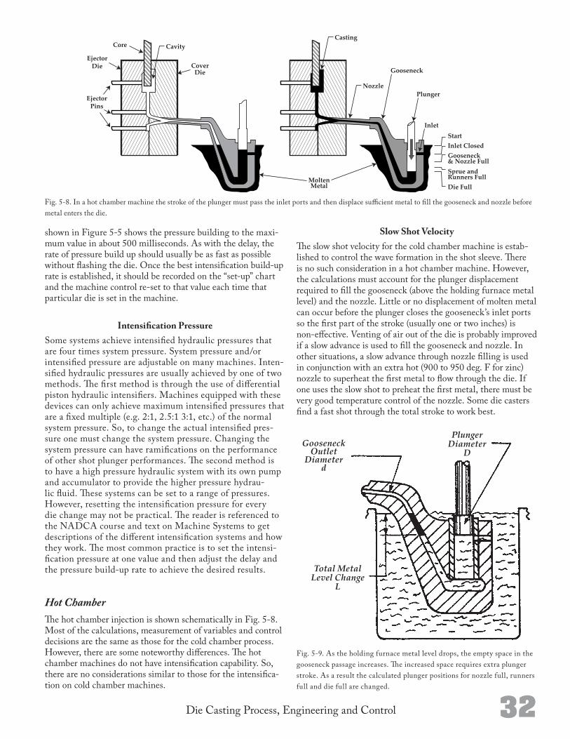
32Die Casting Process, Engineering and Control

Fig. 5­9. As the holding furnace metal level drops, the empty space in the gooseneck passage increases. The increased space requires extra plunger stroke. As a result the calculated plunger positions for nozzle full, runners full and die full are changed.

MoltenMetal

CavityCore

EjectorDie

EjectorPins

CoverDie

Casting

Nozzle

Gooseneck

Plunger

InletStartInlet ClosedGooseneck & Nozzle FullSprue andRunners FullDie Full

Fig. 5­8. In a hot chamber machine the stroke of the plunger must pass the inlet ports and then displace sufficient metal to fill the gooseneck and nozzle before metal enters the die.

shown in Figure 5­5 shows the pressure building to the maxi­mum value in about 500 milliseconds. As with the delay, the rate of pressure build up should usually be as fast as possible without flashing the die. Once the best intensification build­up rate is established, it should be recorded on the “set­up” chart and the machine control re­set to that value each time that particular die is set in the machine.

Intensification PressureSome systems achieve intensified hydraulic pressures that are four times system pressure. System pressure and/or intensified pressure are adjustable on many machines. Inten­sified hydraulic pressures are usually achieved by one of two methods. The first method is through the use of differential piston hydraulic intensifiers. Machines equipped with these devices can only achieve maximum intensified pressures that are a fixed multiple (e.g. 2:1, 2.5:1 3:1, etc.) of the normal system pressure. So, to change the actual intensified pres­sure one must change the system pressure. Changing the system pressure can have ramifications on the performance of other shot plunger performances. The second method is to have a high pressure hydraulic system with its own pump and accumulator to provide the higher pressure hydrau­lic fluid. These systems can be set to a range of pressures. However, resetting the intensification pressure for every die change may not be practical. The reader is referenced to the NADCA course and text on Machine Systems to get descriptions of the different intensification systems and how they work. The most common practice is to set the intensi­fication pressure at one value and then adjust the delay and the pressure build­up rate to achieve the desired results.

Hot ChamberThe hot chamber injection is shown schematically in Fig. 5­8. Most of the calculations, measurement of variables and control decisions are the same as those for the cold chamber process. However, there are some noteworthy differences. The hot chamber machines do not have intensification capability. So, there are no considerations similar to those for the intensifica­tion on cold chamber machines.

Slow Shot VelocityThe slow shot velocity for the cold chamber machine is estab­lished to control the wave formation in the shot sleeve. There is no such consideration in a hot chamber machine. However, the calculations must account for the plunger displacement required to fill the gooseneck (above the holding furnace metal level) and the nozzle. Little or no displacement of molten metal can occur before the plunger closes the gooseneck’s inlet ports so the first part of the stroke (usually one or two inches) is non­effective. Venting of air out of the die is probably improved if a slow advance is used to fill the gooseneck and nozzle. In other situations, a slow advance through nozzle filling is used in conjunction with an extra hot (900 to 950 deg. F for zinc) nozzle to superheat the first metal to flow through the die. If one uses the slow shot to preheat the first metal, there must be very good temperature control of the nozzle. Some die casters find a fast shot through the total stroke to work best.

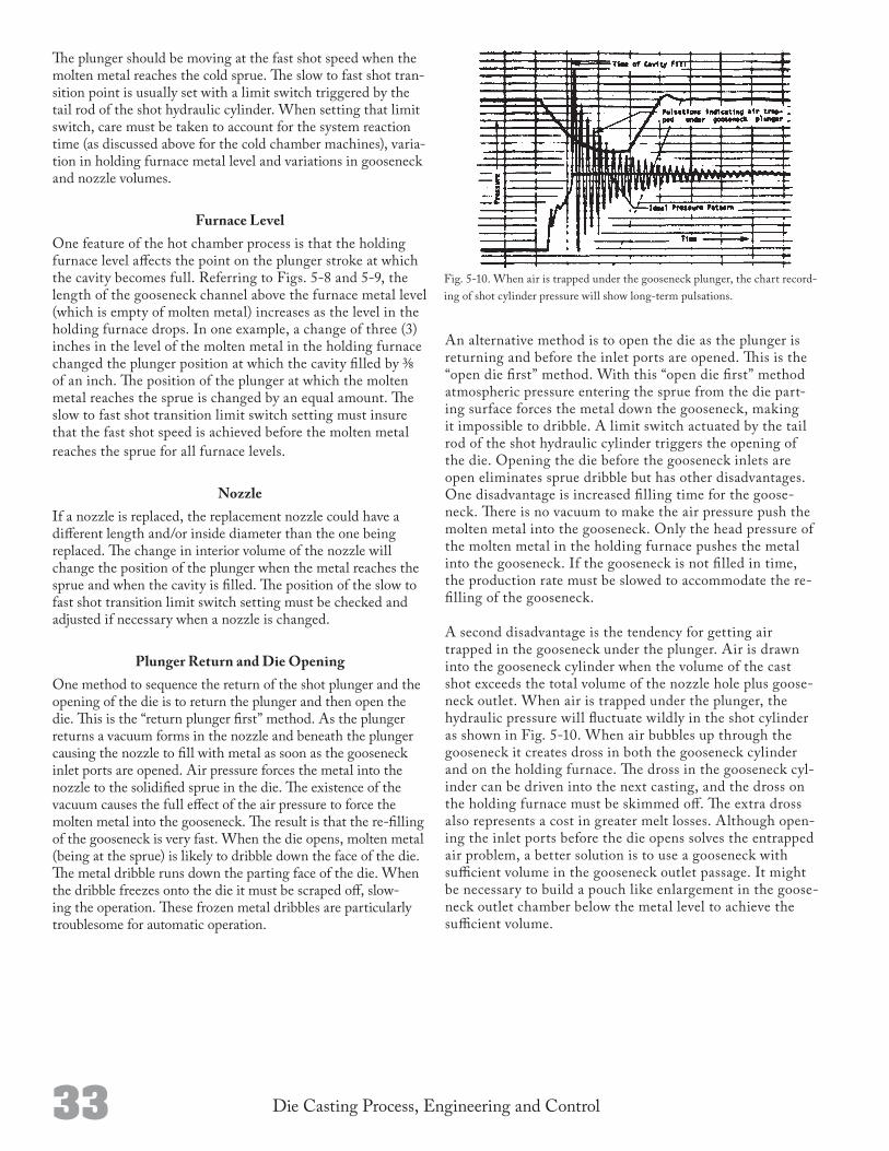
33 Die Casting Process, Engineering and Control

The plunger should be moving at the fast shot speed when the molten metal reaches the cold sprue. The slow to fast shot tran­sition point is usually set with a limit switch triggered by the tail rod of the shot hydraulic cylinder. When setting that limit switch, care must be taken to account for the system reaction time (as discussed above for the cold chamber machines), varia­tion in holding furnace metal level and variations in gooseneck and nozzle volumes.

Furnace LevelOne feature of the hot chamber process is that the holding furnace level affects the point on the plunger stroke at which the cavity becomes full. Referring to Figs. 5­8 and 5­9, the length of the gooseneck channel above the furnace metal level (which is empty of molten metal) increases as the level in the holding furnace drops. In one example, a change of three (3) inches in the level of the molten metal in the holding furnace changed the plunger position at which the cavity filled by 3/8 of an inch. The position of the plunger at which the molten metal reaches the sprue is changed by an equal amount. The slow to fast shot transition limit switch setting must insure that the fast shot speed is achieved before the molten metal reaches the sprue for all furnace levels.

NozzleIf a nozzle is replaced, the replacement nozzle could have a different length and/or inside diameter than the one being replaced. The change in interior volume of the nozzle will change the position of the plunger when the metal reaches the sprue and when the cavity is filled. The position of the slow to fast shot transition limit switch setting must be checked and adjusted if necessary when a nozzle is changed.

Plunger Return and Die OpeningOne method to sequence the return of the shot plunger and the opening of the die is to return the plunger and then open the die. This is the “return plunger first” method. As the plunger returns a vacuum forms in the nozzle and beneath the plunger causing the nozzle to fill with metal as soon as the gooseneck inlet ports are opened. Air pressure forces the metal into the nozzle to the solidified sprue in the die. The existence of the vacuum causes the full effect of the air pressure to force the molten metal into the gooseneck. The result is that the re­filling of the gooseneck is very fast. When the die opens, molten metal (being at the sprue) is likely to dribble down the face of the die. The metal dribble runs down the parting face of the die. When the dribble freezes onto the die it must be scraped off, slow­ing the operation. These frozen metal dribbles are particularly troublesome for automatic operation.

Fig. 5­10. When air is trapped under the gooseneck plunger, the chart record­ing of shot cylinder pressure will show long­term pulsations.

An alternative method is to open the die as the plunger is returning and before the inlet ports are opened. This is the “open die first” method. With this “open die first” method atmospheric pressure entering the sprue from the die part­ing surface forces the metal down the gooseneck, making it impossible to dribble. A limit switch actuated by the tail rod of the shot hydraulic cylinder triggers the opening of the die. Opening the die before the gooseneck inlets are open eliminates sprue dribble but has other disadvantages. One disadvantage is increased filling time for the goose­neck. There is no vacuum to make the air pressure push the molten metal into the gooseneck. Only the head pressure of the molten metal in the holding furnace pushes the metal into the gooseneck. If the gooseneck is not filled in time, the production rate must be slowed to accommodate the re­filling of the gooseneck.

A second disadvantage is the tendency for getting air trapped in the gooseneck under the plunger. Air is drawn into the gooseneck cylinder when the volume of the cast shot exceeds the total volume of the nozzle hole plus goose­neck outlet. When air is trapped under the plunger, the hydraulic pressure will fluctuate wildly in the shot cylinder as shown in Fig. 5­10. When air bubbles up through the gooseneck it creates dross in both the gooseneck cylinder and on the holding furnace. The dross in the gooseneck cyl­inder can be driven into the next casting, and the dross on the holding furnace must be skimmed off. The extra dross also represents a cost in greater melt losses. Although open­ing the inlet ports before the die opens solves the entrapped air problem, a better solution is to use a gooseneck with sufficient volume in the gooseneck outlet passage. It might be necessary to build a pouch like enlargement in the goose­neck outlet chamber below the metal level to achieve the sufficient volume.

Die Casting Process, Engineering and Control 34

The purpose of the clamping system of a die casting machine is to hold the die halves together as the molten metal is injected and to open and close the die for removal of the casting. This chapter addresses the holding together of the die halves.

There are two types of clamping frame structures used on die casting machines. These are the tie bars with platens type and the solid frame type. The tie bar and platen type is used as the example in this chapter because it is the most common, illus­

Clamping Force

Fig. 6­1. The force of the die­close hydraulic cylinder is multiplied by the toggles to stretch the tie bars after the die closes. The amount of tie bar elon­gation is directly related to the clamping force on the die.

C H A P T E R

trates all of the control concepts and it provides for the most possible adjustment. Except for the additional opportunity for adjustment of the individual tie bars on the tie bar and platen type, the two types yield to the same analyses.

The clamp system of a die casting machine is shown in Fig. 6­1 and consists of the platens, tie bars, toggles, and die close cylinder with its attendant hydraulic equipment. The perfor­mance of the clamp system can be analyzed by measuring tie bar strain, rod end hydraulic pressure in the die close cylinder, head end hydraulic pressure in the die close cylinder, and the time intervals between events in the cycle. Casting thickness variation is the most direct result of improper performance of the clamp system. Variations in casting thickness obviously have dimensional effects and they also influence direct material usage and heat input to the die. The dimensional relationships are developed thoroughly in the NADCA textbook Dimen-sional Repeatability of the Die Casting Process. Another, and rather obvious, result of improper performance is when the machine will not “lock up”. In that instance the die will close, but the toggles never straighten so the machine just stalls and does not continue the process sequence. Measurements of the critical variables of the clamp system can also contain clues to problems in the other machine systems.

Computing Required ConditionsThe critical control variables of the clamping system are the tie bar strains (i.e. elongations under load). The required or ideal strains are established by first determining the loads that must be carried and then computing the strain that will result. These loads are calculated in tons of machine clamping force. This clamping tonnage calculation is one of the first calculations the die casting engineer makes when considering a new casting to be made. The hydraulic system of the machine provides the energy to strain the tie bars. The hydraulic pressure in the die close cylinder, the diameter of the cylinder and the mechanical advantage of the toggles create the force to stretch the tie bars.

Computing Tie Bar LoadAs the toggles straighten, they first close the die, and then, as they approach the position of highest mechanical advantage, stretch the tie bars to develop the holding force on the die. The close­clamp sequence is illustrated in Fig. 6­1.

During the original planning and/or die design stage, the expected clamp force should be computed. The required die clamp force is:

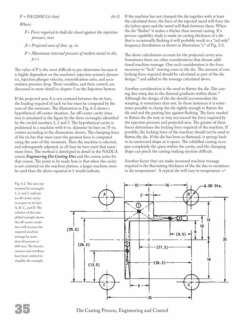
35 Die Casting Process, Engineering and Control

F = PA/(2000 Lb./ton) (6-1)

Where:

F= Force required to hold die closed against the injection pressure, tons

A = Projected area of shot, sq. in.

P = Maximum internal pressure of molten metal in die, p.s.i.

The value of P is the most difficult to pre­determine because it is highly dependent on the machine’s injection system’s dynam­ics, injection plunger velocity, intensification ratio, and accu­mulator pressure drop. These variables, and their control, are discussed in more detail in chapter 5 on the Injection System.

If the projected area A is not centered between the tie bars, the loading required of each tie bar must be computed by the sum­of­the­moments. The illustration in Fig. 6­2 shows a hypothetical off­center situation. An off­center cavity situa­tion is simulated in the figure by the three rectangles identified by the circled numbers 1, 2 and 3. The hypothetical cavity is positioned in a machine with 6­in. diameter tie bars on 35­in. centers according to the dimensions shown. The clamping force of the tie bar that must exert the greatest force is computed using the sum­of­the­moments. Then the machine is selected, and subsequently adjusted, so all four tie bars exert that maxi­mum force. The method is developed in detail in the NADCA course Engineering Die Casting Dies and the course notes for that course. The point to be made here is that when the cavity is not centered on the machine platens, a larger machine must be used than the above equation 6­1 would indicate.

If the machine has not clamped the die together with at least the calculated force, the force of the injected metal will force the die halves apart and the metal will flash between them. When the die “flashes” it makes a thicker than normal casting. If a process capability study is made on casting thickness of a die that is occasionally flashing it will probably result in a “tail only” frequency distribution as shown in illustration “e” of Fig. 2­2.

The above calculations account for the projected cavity area. Sometimes there are other considerations that dictate addi­tional machine tonnage. One such consideration is the force necessary to “lock” moving cores in the die. The amount of core locking force required should be calculated as part of the die design,24 and added to the tonnage calculated above.

Another consideration is the need to flatten the die. Die cast­ing dies warp due to the thermal gradients within them.24 Although the design of the die should accommodate the warping, it sometimes does not. In those instances it is some­times possible to clamp the die tightly enough to flatten the die and seal the parting line against flashing. The force needed to flatten the die may or may not exceed the force required by the injection pressure and projected area. The greater of these forces determines the locking force required of the machine. If possible, the locking force of the machine should not be used to flatten the die. If the die has been so flattened, it springs back to its unstressed shape as it opens. The solidified casting occu­pies completely the space within the cavity, and the changing shape can pinch the casting making ejection difficult.

Another factor that can make increased machine tonnage required is the fluctuating thickness of the die due to variations in die temperature1. A typical die will vary in temperature +/­

Fig. 6­2. The area rep­resented by rectangles 1, 2, and 3, indicate an off­center cavity in respect to tie bars A, B, C, and D. The solution of this sim­plified example shows the off­center condi­tion will increase the required machine tonnage by more than 60 percent to 600 tons. The biscuit, runners and overflows have been omitted to simplify the example.

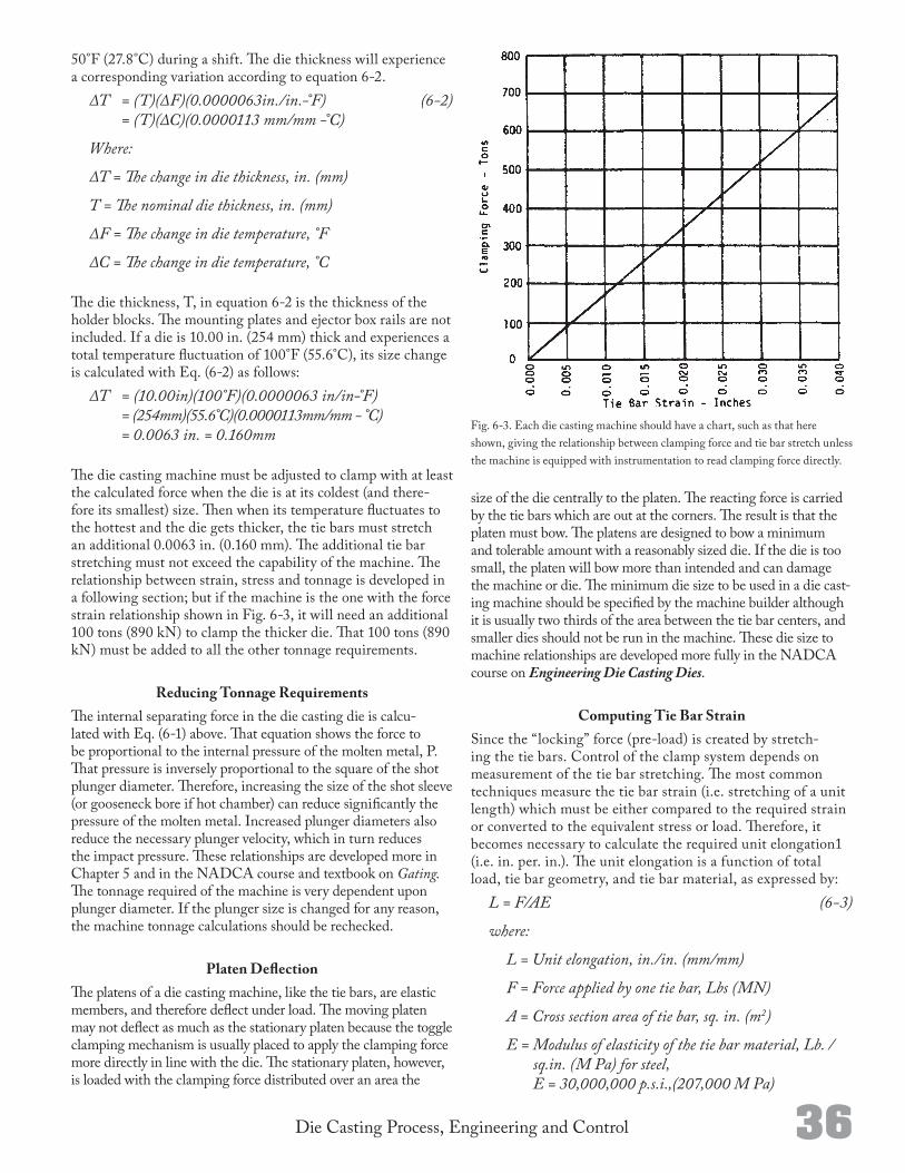
36Die Casting Process, Engineering and Control

50°F (27.8°C) during a shift. The die thickness will experience a corresponding variation according to equation 6­2.

ΔT = (T)(ΔF)(0.0000063in./in.-°F) (6-2) = (T)(ΔC)(0.0000113 mm/mm -°C)

Where:

ΔT = The change in die thickness, in. (mm)

T = The nominal die thickness, in. (mm)

ΔF = The change in die temperature, °F

ΔC = The change in die temperature, °C

The die thickness, T, in equation 6­2 is the thickness of the holder blocks. The mounting plates and ejector box rails are not included. If a die is 10.00 in. (254 mm) thick and experiences a total temperature fluctuation of 100°F (55.6°C), its size change is calculated with Eq. (6­2) as follows:

ΔT = (10.00in)(100°F)(0.0000063 in/in-°F) = (254mm)(55.6°C)(0.0000113mm/mm - °C) = 0.0063 in. = 0.160mm

The die casting machine must be adjusted to clamp with at least the calculated force when the die is at its coldest (and there­fore its smallest) size. Then when its temperature fluctuates to the hottest and the die gets thicker, the tie bars must stretch an additional 0.0063 in. (0.160 mm). The additional tie bar stretching must not exceed the capability of the machine. The relationship between strain, stress and tonnage is developed in a following section; but if the machine is the one with the force strain relationship shown in Fig. 6­3, it will need an additional 100 tons (890 kN) to clamp the thicker die. That 100 tons (890 kN) must be added to all the other tonnage requirements.

Reducing Tonnage RequirementsThe internal separating force in the die casting die is calcu­lated with Eq. (6­1) above. That equation shows the force to be proportional to the internal pressure of the molten metal, P. That pressure is inversely proportional to the square of the shot plunger diameter. Therefore, increasing the size of the shot sleeve (or gooseneck bore if hot chamber) can reduce significantly the pressure of the molten metal. Increased plunger diameters also reduce the necessary plunger velocity, which in turn reduces the impact pressure. These relationships are developed more in Chapter 5 and in the NADCA course and textbook on Gating. The tonnage required of the machine is very dependent upon plunger diameter. If the plunger size is changed for any reason, the machine tonnage calculations should be rechecked.

Platen DeflectionThe platens of a die casting machine, like the tie bars, are elastic members, and therefore deflect under load. The moving platen may not deflect as much as the stationary platen because the toggle clamping mechanism is usually placed to apply the clamping force more directly in line with the die. The stationary platen, however, is loaded with the clamping force distributed over an area the

size of the die centrally to the platen. The reacting force is carried by the tie bars which are out at the corners. The result is that the platen must bow. The platens are designed to bow a minimum and tolerable amount with a reasonably sized die. If the die is too small, the platen will bow more than intended and can damage the machine or die. The minimum die size to be used in a die cast­ing machine should be specified by the machine builder although it is usually two thirds of the area between the tie bar centers, and smaller dies should not be run in the machine. These die size to machine relationships are developed more fully in the NADCA course on Engineering Die Casting Dies.

Computing Tie Bar StrainSince the “locking” force (pre­load) is created by stretch­ing the tie bars. Control of the clamp system depends on measurement of the tie bar stretching. The most common techniques measure the tie bar strain (i.e. stretching of a unit length) which must be either compared to the required strain or converted to the equivalent stress or load. Therefore, it becomes necessary to calculate the required unit elongation1 (i.e. in. per. in.). The unit elongation is a function of total load, tie bar geometry, and tie bar material, as expressed by:

L = F/AE (6-3)

where:

L = Unit elongation, in./in. (mm/mm)

F = Force applied by one tie bar, Lbs (MN)

A = Cross section area of tie bar, sq. in. (m2)

E = Modulus of elasticity of the tie bar material, Lb. /sq.in. (M Pa) for steel, E = 30,000,000 p.s.i.,(207,000 M Pa)

Fig. 6­3. Each die casting machine should have a chart, such as that here shown, giving the relationship between clamping force and tie bar stretch unless the machine is equipped with instrumentation to read clamping force directly.

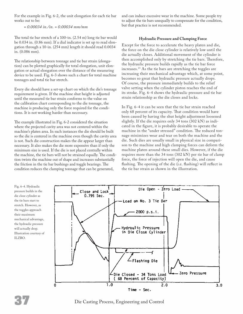
37 Die Casting Process, Engineering and Control

For the example in Fig. 6­2, the unit elongation for each tie bar works out to be:

= 0.00034 in./in. = 0.00034 mm/mm

The total tie bar stretch of a 100­in. (2.54 m) long tie bar would be 0.034 in. (0.86 mm). If a dial indicator is set up to read elon­gation through a 10­in. (254 mm) length it should read 0.0034 in. (0.086 mm).

The relationship between tonnage and tie bar strain (elonga­tion) can be plotted graphically for total elongation, unit elon­gation or actual elongation over the distance of the measuring device to be used. Fig. 6­3 shows such a chart for total machine tonnages and total tie bar stretch.

Every die should have a set­up chart on which the die’s tonnage requirement is given. If the machine shut height is adjusted until the measured tie bar strain conforms to the value on the calibration chart corresponding to the die tonnage, the machine is producing only the force required for the condi­tions. It is not working harder than necessary.

The example illustrated in Fig. 6­2 considered the situation where the projected cavity area was not centered within the machine’s platen area. In such instances the die should be built so the die is centered in the machine even though the cavity area is not. Such die construction makes the die appear larger than necessary. It also makes the die more expensive than if only the minimum size is used. If the die is not placed centrally within the machine, the tie bars will not be strained equally. The condi­tion twists the machine out of shape and increases substantially the friction in the tie bar bushings and toggle bearings. The condition reduces the clamping tonnage that can be generated,

and can induce excessive wear in the machine. Some people try to adjust the tie bars unequally to compensate for the condition, but that practice is not recommended.

Hydraulic Pressure and Clamping ForceExcept for the force to accelerate the heavy platen and die, the force on the die close cylinder is relatively low until the die actually closes. Additional movement of the cylinder is then accomplished only by stretching the tie bars. Therefore, the hydraulic pressure builds rapidly as the tie bar force increases.23 As the tie bars are stretching the toggles are increasing their mechanical advantage which, at some point, becomes so great that hydraulic pressure actually drops. Of course, the pressure immediately builds to the relief valve setting when the cylinder piston reaches the end of its stroke. Fig. 6­4 shows the hydraulic pressure and tie bar strain relationship as the die closes and locks.

In Fig. 6­4 it can be seen that the tie bar strain reached only 68 percent of its capacity. That condition would have been caused by having the shut height adjustment loosened slightly. If the die requires only 34 tons (302 kN) as indi­cated in the figure, it is probably desirable to operate the machine in the “under stressed” condition. The reduced ton­nage minimizes wear and tear on both the machine and the die. Such dies are usually small in physical size in compari­son to the machine and high clamping forces can deform the machine platen around these small dies. However, if the die requires more than the 34 tons (302 kN) per tie bar of clamp force, the force of injection will open the die, and cause flashing. The opening of the die (i.e. flashing) will reflect in the tie bar strain as shown in the illustration.

Fig. 6­4. Hydraulic pressure builds in the die close cylinder as the tie bars start to stretch. However, as the toggles approach their maximum mechanical advantage, the hydraulic pressure will actually drop. Illustration courtesy of ILZRO.

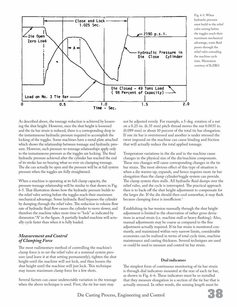
38Die Casting Process, Engineering and Control

As described above, the tonnage reduction is achieved by loosen­ing the shut height. However, once the shut height is loosened and the tie bar strain is reduced, there is a corresponding drop in the instantaneous hydraulic pressure required to accomplish the locking of the toggles. Some machines have a metal plate attached which shows the relationship between tonnage and hydraulic pres­sure. However, such pressure­to­tonnage relationships apply only to the instantaneous pressure as the toggles are locking. The final hydraulic pressure achieved after the cylinder has reached the end of its stroke has no bearing what­so­ever on clamping tonnage. The die can actually be open and the pressure will be at full system pressure when the toggles are fully straightened.

When a machine is operating at its full clamp capacity, the pressure­tonnage relationship will be similar to that shown in Fig. 6­5. That illustration shows how the hydraulic pressure builds to the relief valve setting before the toggles reach their maximum mechanical advantage. Some hydraulic fluid bypasses the cylinder by dumping through the relief valve. The reduction in volume flow rate of hydraulic fluid flow causes the cylinder to move slower, and therefore the machine takes more time to “lock” as indicated by dimension “A” in the figure. A partially­loaded machine will actu­ally cycle faster than when it is fully loaded.

Measurement and Control of Clamping ForceThe most rudimentary method of controlling the machine’s clamp force is to set the relief valve at a nominal system pres­sure (and leave it at that setting permanently), tighten the shut height until the machine will not lock, and then loosen the shut height until the machine will just lock. This technique may insure maximum clamp force for a few shots.

Several factors can cause undetectable variation in the tonnage when the above technique is used. First, the tie bar nuts may

not be adjusted evenly. For example, a 5­deg. rotation of a nut on a 0.25­in. (6.35 mm) pitch thread moves the nut 0.0035 in. (0.089 mm) or about 10 percent of the total tie bar elongation. If one tie bar is overstressed and another is under stressed the twist imposed on the machine can cause binding and friction that will actually reduce the total applied tonnage.

Temperature variations in the die and in the machine cause changes in the physical size of the die/machine components. These size changes will cause corresponding changes in the tie bar strain. The most obvious effect of this type of situation is when a die warms­up, expands, and hence requires more tie bar elongation than the clamp cylinder/toggle system can provide. The clamp system then stalls. All hydraulic fluid dumps over the relief valve, and the cycle is interrupted. The practical approach then is to back­off the shut height adjustment to compensate for the larger die. If the die should then cool somewhat, it may flash because clamping force is insufficient.1

Establishing tie bar tension manually through the shut height adjustment is limited to the observation of rather gross devia­tions in actual strain (i.e. machine stall or heavy flashing). Also, manual adjustments may be coarse as compared to the fine adjustment actually required. If tie bar strain is monitored con­stantly, and maintained within very narrow limits, considerable economies can be realized in terms of total cycle time, machine maintenance and casting thickness. Several techniques are used or could be used to measure and control tie bar strain.

Dial indicatorsThe simplest form of continuous monitoring of tie bar strain is through dial indicators mounted at the rear of each tie bar, as shown in Fig. 6­6. These indicators must be so installed that they measure elongation in a section of the tie bar that is actually stressed. In other words, the sensing length must be

Fig. 6­5. When hydraulic pressure must build to the relief valve setting before the toggles reach their maximum mechanical advantage, some fluid passes through the relief valve extending the machine cycle time. Illustration courtesy of ILZRO.

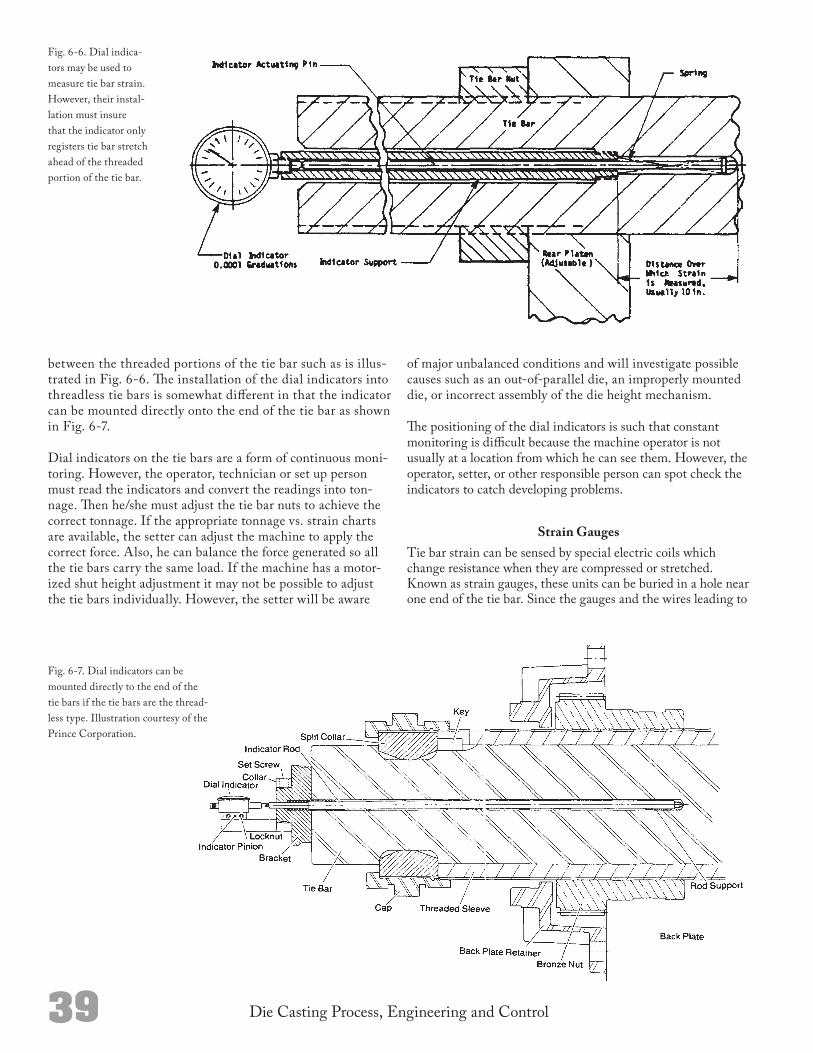
39 Die Casting Process, Engineering and Control

between the threaded portions of the tie bar such as is illus­trated in Fig. 6­6. The installation of the dial indicators into threadless tie bars is somewhat different in that the indicator can be mounted directly onto the end of the tie bar as shown in Fig. 6­7.

Dial indicators on the tie bars are a form of continuous moni­toring. However, the operator, technician or set up person must read the indicators and convert the readings into ton­nage. Then he/she must adjust the tie bar nuts to achieve the correct tonnage. If the appropriate tonnage vs. strain charts are available, the setter can adjust the machine to apply the correct force. Also, he can balance the force generated so all the tie bars carry the same load. If the machine has a motor­ized shut height adjustment it may not be possible to adjust the tie bars individually. However, the setter will be aware

of major unbalanced conditions and will investigate possible causes such as an out­of­parallel die, an improperly mounted die, or incorrect assembly of the die height mechanism.

The positioning of the dial indicators is such that constant monitoring is difficult because the machine operator is not usually at a location from which he can see them. However, the operator, setter, or other responsible person can spot check the indicators to catch developing problems.

Strain GaugesTie bar strain can be sensed by special electric coils which change resistance when they are compressed or stretched. Known as strain gauges, these units can be buried in a hole near one end of the tie bar. Since the gauges and the wires leading to

Fig. 6­6. Dial indica­tors may be used to measure tie bar strain. However, their instal­lation must insure that the indicator only registers tie bar stretch ahead of the threaded portion of the tie bar.

Fig. 6­7. Dial indicators can be mounted directly to the end of the tie bars if the tie bars are the thread­less type. Illustration courtesy of the Prince Corporation.

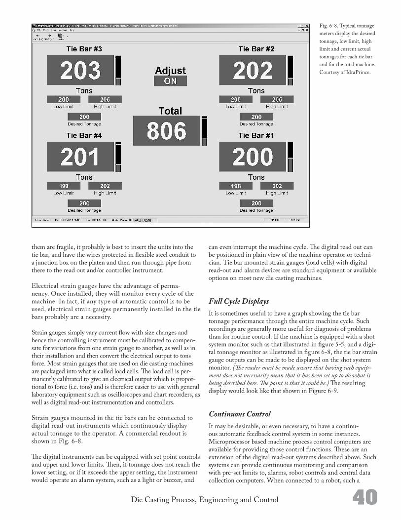
40Die Casting Process, Engineering and Control

them are fragile, it probably is best to insert the units into the tie bar, and have the wires protected in flexible steel conduit to a junction box on the platen and then run through pipe from there to the read out and/or controller instrument.

Electrical strain gauges have the advantage of perma­nency. Once installed, they will monitor every cycle of the machine. In fact, if any type of automatic control is to be used, electrical strain gauges permanently installed in the tie bars probably are a necessity.

Strain gauges simply vary current flow with size changes and hence the controlling instrument must be calibrated to compen­sate for variations from one strain gauge to another, as well as in their installation and then convert the electrical output to tons force. Most strain gauges that are used on die casting machines are packaged into what is called load cells. The load cell is per­manently calibrated to give an electrical output which is propor­tional to force (i.e. tons) and is therefore easier to use with general laboratory equipment such as oscilloscopes and chart recorders, as well as digital read­out instrumentation and controllers.

Strain gauges mounted in the tie bars can be connected to digital read­out instruments which continuously display actual tonnage to the operator. A commercial readout is shown in Fig. 6­8.

The digital instruments can be equipped with set point controls and upper and lower limits. Then, if tonnage does not reach the lower setting, or if it exceeds the upper setting, the instrument would operate an alarm system, such as a light or buzzer, and

Fig. 6­8. Typical tonnage meters display the desired tonnage, low limit, high limit and current actual tonnages for each tie bar and for the total machine. Courtesy of IdraPrince.

can even interrupt the machine cycle. The digital read out can be positioned in plain view of the machine operator or techni­cian. Tie bar mounted strain gauges (load cells) with digital read­out and alarm devices are standard equipment or available options on most new die casting machines.

Full Cycle DisplaysIt is sometimes useful to have a graph showing the tie bar tonnage performance through the entire machine cycle. Such recordings are generally more useful for diagnosis of problems than for routine control. If the machine is equipped with a shot system monitor such as that illustrated in figure 5­5, and a digi­tal tonnage monitor as illustrated in figure 6­8, the tie bar strain gauge outputs can be made to be displayed on the shot system monitor. (The reader must be made aware that having such equip-ment does not necessarily mean that it has been set up to do what is being described here. The point is that it could be.) The resulting display would look like that shown in Figure 6­9.

Continuous ControlIt may be desirable, or even necessary, to have a continu­ous automatic feedback control system in some instances. Microprocessor based machine process control computers are available for providing those control functions. These are an extension of the digital read­out systems described above. Such systems can provide continuous monitoring and comparison with pre­set limits to, alarms, robot controls and central data collection computers. When connected to a robot, such a

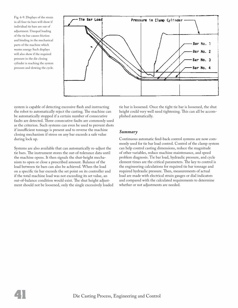
41 Die Casting Process, Engineering and Control

system is capable of detecting excessive flash and instructing the robot to automatically reject the casting. The machine can be automatically stopped if a certain number of consecutive faults are detected. Three consecutive faults are commonly used as the criterion. Such systems can even be used to prevent shots if insufficient tonnage is present and to reverse the machine closing mechanism if stress on any bar exceeds a safe value during lock up.

Systems are also available that can automatically re­adjust the tie bars. The instrument stores the out­of­tolerance data until the machine opens. It then signals the shut­height mecha­nism to open or close a prescribed amount. Balance of the load between tie bars can also be achieved. When the load on a specific tie bar exceeds the set point on its controller and if the total machine load was not exceeding its set value, an out­of­balance condition would exist. The shut height adjust­ment should not be loosened, only the single excessively loaded

Fig. 6­9. Displays of the strain in all four tie bars will show if individual tie bars are out of adjustment. Unequal loading of the tie bar causes friction and binding in the mechanical parts of the machine which wastes energy Such displays will also show if the required pressure in the die closing cylinder is reaching the system pressure and slowing the cycle.

tie bar is loosened. Once the tight tie bar is loosened, the shut height could very well need tightening. This can all be accom­plished automatically.

SummaryContinuous automatic feed­back control systems are now com­monly used for tie bar load control. Control of the clamp system can help control casting dimensions, reduce the magnitude of other variables, reduce machine maintenance, and speed problem diagnosis. Tie bar load, hydraulic pressure, and cycle element times are the critical parameters. The key to control is the engineering calculations for required tie bar tonnage and required hydraulic pressure. Then, measurements of actual load are made with electrical strain gauges or dial indicators and compared with the calculated requirements to determine whether or not adjustments are needed.

Die Casting Process, Engineering and Control 42

The flow of heat from the metal being cast determines the solidification pattern within the casting. If solidification progresses properly a usable casting results. However, if the wrong solidification pattern develops, the resulting casting must be scrapped. Die casting is therefore a thermal process. The control of the thermodynamics of the process is all that really matters. Much emphasis is placed on gating theory and injection control, but even those efforts are actually to establish the best possible initial thermal condition. It can be concluded that casting/die temperature control is the most important consideration in process control. A thorough discussion of the heat flow phenomenon3 is beyond the scope of this book. These phenomenon are developed in detail in the NADCA courses and textbooks on Die Casting Dies: Designing and Engineering Die Cooling Systems. How­ever, the temperature patterns that exist within the casting and die must be understood and therefore a certain amount of explanation is unavoidable. Techniques for measuring temperature patterns are described in this chapter, as are the means of controlling those patterns.

The goal is to have control of the transient temperature condition in each casting as it is solidifying and cooling in the die. Those transient thermal conditions drive the solidi­fication patterns and hence the distribution of porsity in the casting. The control of heat flow through the die is actually an indirect method of controlling the transient conditions during casting solidification.3

In one way or another all process variables are related to the transient heat flows during solidification. Cavity fill time and compaction pressure have been defined previously in terms of solidification requirements or behavior. Plunger velocity, tie bar strain, and hydraulic pressures are actually means to achieve the needed fill time and cavity pressure which in turn achieves the necessary thermal pattern or compensates for incorrect thermal patterns in the solidifying casting.

Die temperature is actually a pattern of temperatures. When operating properly, the die will have various temperatures across the parting surface. The sprue or biscuit area should probably be somewhat colder than the cavity area. And, the outermost extremities of the cavity should be hotter than near the gate. Similarly, the die gets colder at greater distances into the die steel from the cavity surface. The coldest areas are immediately adjacent to the water cooling lines and/or at the outside surfaces.

The average die temperature is effected by several other vari­ables. Cycle timing, metal temperature, shot speed and die

Die TemperatureC H A P T E R

blow (flashing) variations can change the average die tempera­ture or the pattern of the die temperature. It is usually more cost effective to control die temperature directly than to control all, or most, of the other variables that affect it.

Traditionally die temperature control was left to the machine operator. However, the operator was never told what the temperature should be, now was he given the means to know what it was. The operator was expected to look at the cast­ings being made and interpret texture, warping or sticking to make temperature related decisions. Depending on how he interpreted what he saw on the casting, he would speed up or slow down, change the application or release material or adjust the cooling water flow. Fortunately there are better tools today for the control of die temperature.

Determining RequirementsThe die temperature requirements for a specific die are

determined during the die design activity. The preciseness with which those requirements are established depends on the technique employed by the die designer. The techniques actu­ally used are:

1. Casual

2. Informed experience

3. Basic heat balance

4. Finite element analysis (FEA)

Each of these techniques are described in the following para­graphs so the process control engineer will understand what he must look for in each die before planning his control strategy.

Casual

The casual approach to the thermal design of the die cast­ing die is to let the die builder drill waterlines wherever he wishes. The die builder should not be expected to understand the nature of heat flow3 as that is not his trade. Even when the die builder does understand the heat flow considerations, he is faced with the conflict of doing what is correct from a heat flow point of view and building the die in the most cost effective way. Usually cost effectiveness wins. The result is a die with few water­lines that are too long and go through the wrong places. In many instances a single waterline will have many inches of length where no cooling is needed and only a short portion

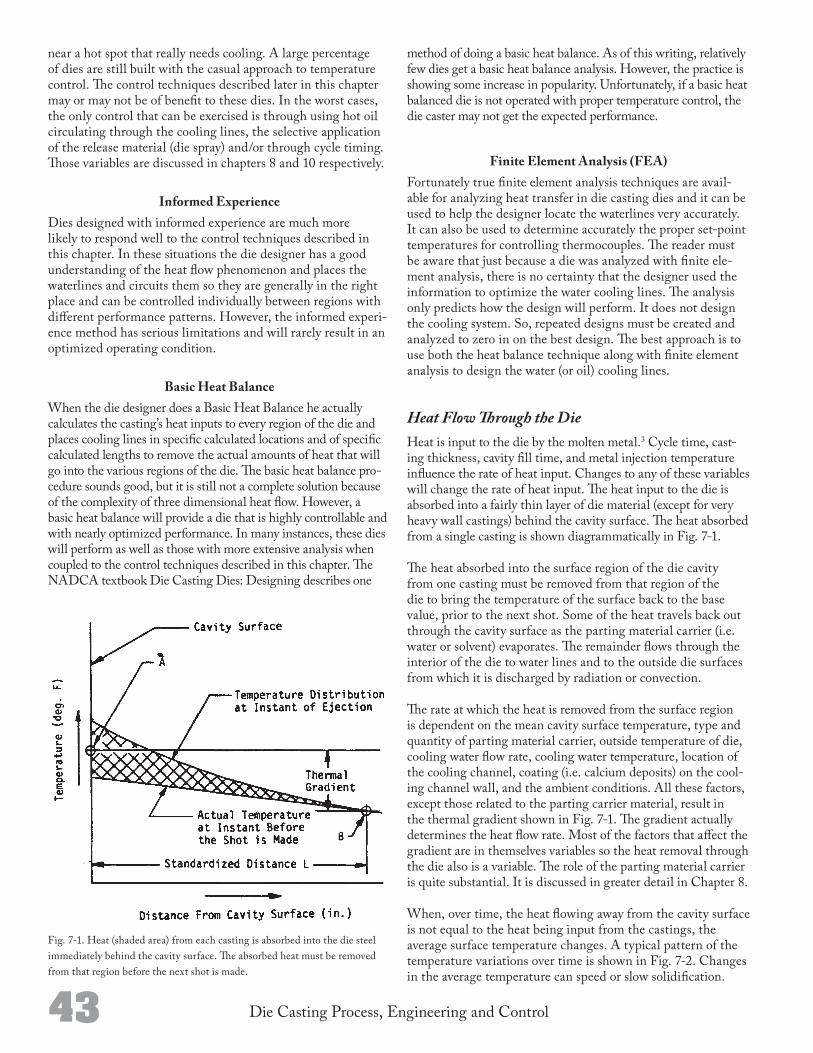
43 Die Casting Process, Engineering and Control

Fig. 7­1. Heat (shaded area) from each casting is absorbed into the die steel immediately behind the cavity surface. The absorbed heat must be removed from that region before the next shot is made.

near a hot spot that really needs cooling. A large percentage of dies are still built with the casual approach to temperature control. The control techniques described later in this chapter may or may not be of benefit to these dies. In the worst cases, the only control that can be exercised is through using hot oil circulating through the cooling lines, the selective application of the release material (die spray) and/or through cycle timing. Those variables are discussed in chapters 8 and 10 respectively.

Informed ExperienceDies designed with informed experience are much more likely to respond well to the control techniques described in this chapter. In these situations the die designer has a good understanding of the heat flow phenomenon and places the waterlines and circuits them so they are generally in the right place and can be controlled individually between regions with different performance patterns. However, the informed experi­ence method has serious limitations and will rarely result in an optimized operating condition.

Basic Heat BalanceWhen the die designer does a Basic Heat Balance he actually calculates the casting’s heat inputs to every region of the die and places cooling lines in specific calculated locations and of specific calculated lengths to remove the actual amounts of heat that will go into the various regions of the die. The basic heat balance pro­cedure sounds good, but it is still not a complete solution because of the complexity of three dimensional heat flow. However, a basic heat balance will provide a die that is highly controllable and with nearly optimized performance. In many instances, these dies will perform as well as those with more extensive analysis when coupled to the control techniques described in this chapter. The NADCA textbook Die Casting Dies: Designing describes one

method of doing a basic heat balance. As of this writing, relatively few dies get a basic heat balance analysis. However, the practice is showing some increase in popularity. Unfortunately, if a basic heat balanced die is not operated with proper temperature control, the die caster may not get the expected performance.

Finite Element Analysis (FEA)Fortunately true finite element analysis techniques are avail­able for analyzing heat transfer in die casting dies and it can be used to help the designer locate the waterlines very accurately. It can also be used to determine accurately the proper set­point temperatures for controlling thermocouples. The reader must be aware that just because a die was analyzed with finite ele­ment analysis, there is no certainty that the designer used the information to optimize the water cooling lines. The analysis only predicts how the design will perform. It does not design the cooling system. So, repeated designs must be created and analyzed to zero in on the best design. The best approach is to use both the heat balance technique along with finite element analysis to design the water (or oil) cooling lines.

Heat Flow Through the DieHeat is input to the die by the molten metal.3 Cycle time, cast­ing thickness, cavity fill time, and metal injection temperature influence the rate of heat input. Changes to any of these variables will change the rate of heat input. The heat input to the die is absorbed into a fairly thin layer of die material (except for very heavy wall castings) behind the cavity surface. The heat absorbed from a single casting is shown diagrammatically in Fig. 7­1.

The heat absorbed into the surface region of the die cavity from one casting must be removed from that region of the die to bring the temperature of the surface back to the base value, prior to the next shot. Some of the heat travels back out through the cavity surface as the parting material carrier (i.e. water or solvent) evaporates. The remainder flows through the interior of the die to water lines and to the outside die surfaces from which it is discharged by radiation or convection.

The rate at which the heat is removed from the surface region is dependent on the mean cavity surface temperature, type and quantity of parting material carrier, outside temperature of die, cooling water flow rate, cooling water temperature, location of the cooling channel, coating (i.e. calcium deposits) on the cool­ing channel wall, and the ambient conditions. All these factors, except those related to the parting carrier material, result in the thermal gradient shown in Fig. 7­1. The gradient actually determines the heat flow rate. Most of the factors that affect the gradient are in themselves variables so the heat removal through the die also is a variable. The role of the parting material carrier is quite substantial. It is discussed in greater detail in Chapter 8.

When, over time, the heat flowing away from the cavity surface is not equal to the heat being input from the castings, the average surface temperature changes. A typical pattern of the temperature variations over time is shown in Fig. 7­2. Changes in the average temperature can speed or slow solidification.

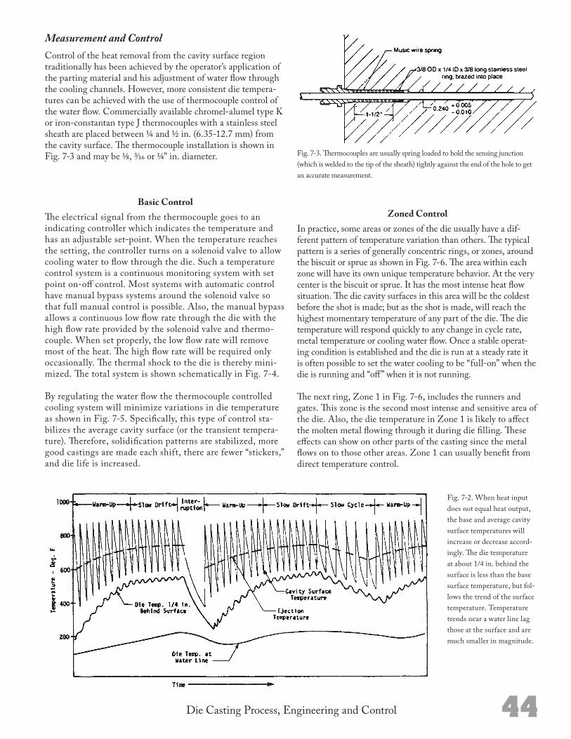
44Die Casting Process, Engineering and Control

Fig. 7­2. When heat input does not equal heat output, the base and average cavity surface temperatures will increase or decrease accord­ingly. The die temperature at about 1/4 in. behind the surface is less than the base surface temperature, but fol­lows the trend of the surface temperature. Temperature trends near a water line lag those at the surface and are much smaller in magnitude.

Fig. 7­3. Thermocouples are usually spring loaded to hold the sensing junction (which is welded to the tip of the sheath) tightly against the end of the hole to get an accurate measurement.

Measurement and ControlControl of the heat removal from the cavity surface region traditionally has been achieved by the operator’s application of the parting material and his adjustment of water flow through the cooling channels. However, more consistent die tempera­tures can be achieved with the use of thermocouple control of the water flow. Commercially available chromel­alumel type K or iron­constantan type J thermocouples with a stainless steel sheath are placed between 1/4 and 1/2 in. (6.35­12.7 mm) from the cavity surface. The thermocouple installation is shown in Fig. 7­3 and may be 1/8, 3/16 or 1/4” in. diameter.

Basic ControlThe electrical signal from the thermocouple goes to an indicating controller which indicates the temperature and has an adjustable set­point. When the temperature reaches the setting, the controller turns on a solenoid valve to allow cooling water to flow through the die. Such a temperature control system is a continuous monitoring system with set point on­off control. Most systems with automatic control have manual bypass systems around the solenoid valve so that full manual control is possible. Also, the manual bypass allows a continuous low flow rate through the die with the high flow rate provided by the solenoid valve and thermo­couple. When set properly, the low flow rate will remove most of the heat. The high flow rate will be required only occasionally. The thermal shock to the die is thereby mini­mized. The total system is shown schematically in Fig. 7­4.

By regulating the water flow the thermocouple controlled cooling system will minimize variations in die temperature as shown in Fig. 7­5. Specifically, this type of control sta­bilizes the average cavity surface (or the transient tempera­ture). Therefore, solidification patterns are stabilized, more good castings are made each shift, there are fewer “stickers,” and die life is increased.

Zoned ControlIn practice, some areas or zones of the die usually have a dif­ferent pattern of temperature variation than others. The typical pattern is a series of generally concentric rings, or zones, around the biscuit or sprue as shown in Fig. 7­6. The area within each zone will have its own unique temperature behavior. At the very center is the biscuit or sprue. It has the most intense heat flow situation. The die cavity surfaces in this area will be the coldest before the shot is made; but as the shot is made, will reach the highest momentary temperature of any part of the die. The die temperature will respond quickly to any change in cycle rate, metal temperature or cooling water flow. Once a stable operat­ing condition is established and the die is run at a steady rate it is often possible to set the water cooling to be “full­on” when the die is running and “off” when it is not running.

The next ring, Zone 1 in Fig. 7­6, includes the runners and gates. This zone is the second most intense and sensitive area of the die. Also, the die temperature in Zone 1 is likely to affect the molten metal flowing through it during die filling. These effects can show on other parts of the casting since the metal flows on to those other areas. Zone 1 can usually benefit from direct temperature control.

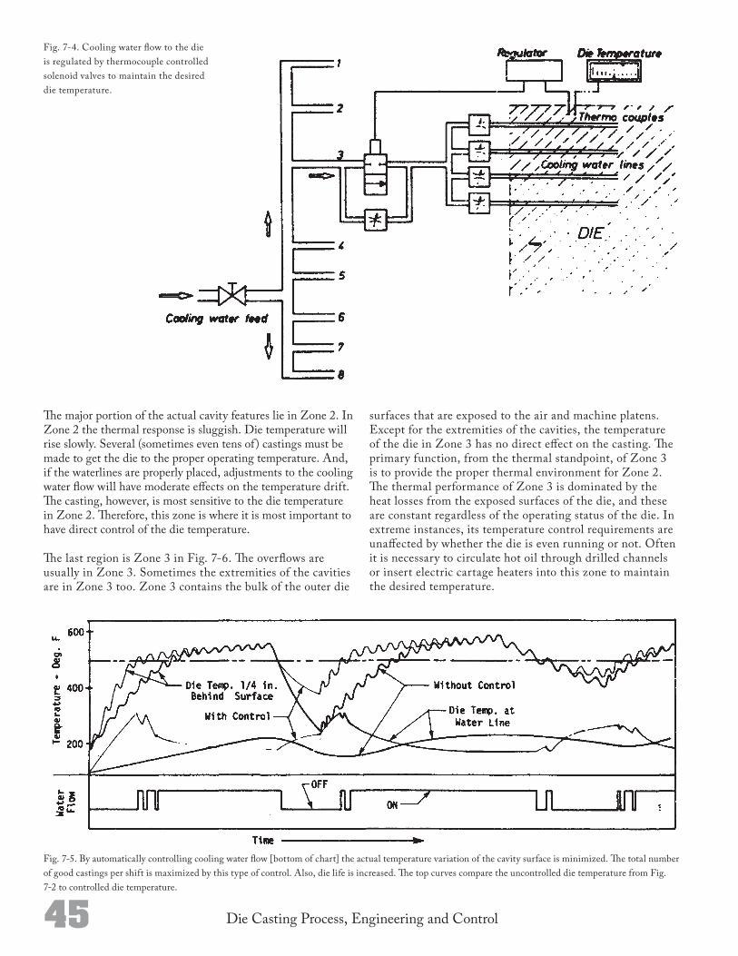
45 Die Casting Process, Engineering and Control

Fig. 7­4. Cooling water flow to the die is regulated by thermocouple controlled solenoid valves to maintain the desired die temperature.

Fig. 7­5. By automatically controlling cooling water flow [bottom of chart] the actual temperature variation of the cavity surface is minimized. The total number of good castings per shift is maximized by this type of control. Also, die life is increased. The top curves compare the uncontrolled die temperature from Fig. 7­2 to controlled die temperature.

The major portion of the actual cavity features lie in Zone 2. In Zone 2 the thermal response is sluggish. Die temperature will rise slowly. Several (sometimes even tens of) castings must be made to get the die to the proper operating temperature. And, if the waterlines are properly placed, adjustments to the cooling water flow will have moderate effects on the temperature drift. The casting, however, is most sensitive to the die temperature in Zone 2. Therefore, this zone is where it is most important to have direct control of the die temperature.

The last region is Zone 3 in Fig. 7­6. The overflows are usually in Zone 3. Sometimes the extremities of the cavities are in Zone 3 too. Zone 3 contains the bulk of the outer die

surfaces that are exposed to the air and machine platens. Except for the extremities of the cavities, the temperature of the die in Zone 3 has no direct effect on the casting. The primary function, from the thermal standpoint, of Zone 3 is to provide the proper thermal environment for Zone 2. The thermal performance of Zone 3 is dominated by the heat losses from the exposed surfaces of the die, and these are constant regardless of the operating status of the die. In extreme instances, its temperature control requirements are unaffected by whether the die is even running or not. Often it is necessary to circulate hot oil through drilled channels or insert electric cartage heaters into this zone to maintain the desired temperature.

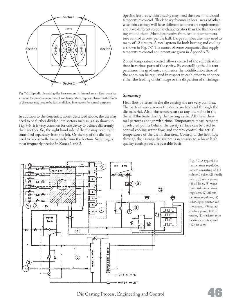
46Die Casting Process, Engineering and Control

Fig. 7­6. Typically die casting dies have concentric thermal zones. Each zone has a unique temperature requirement and temperature response characteristic. Some of the zones may need to be further divided into sectors for control purposes.

Fig. 7­7. A typical die temperature regulation system consisting of: (1) solenoid valve, (2) needle valve, (3) water pump, (4) oil lines, (5) water lines, (6) temperature regulator, (7) oil tem­perature regulator, (8) submerged resistor and thermostat, (9) sealed cooling pump, (10) oil pump, (11) resistor­type heating chamber, and (12) air vents.

In addition to the concentric zones described above, the die may need to be further divided into sectors such as is also shown in Fig. 7­6. It is very common for one cavity to behave differently than another. So, the right hand side of the die may need to be controlled separately from the left. Or the top of the die may need to be controlled separately from the bottom. Sectoring is most frequently needed in Zones 1 and 2.

Specific features within a cavity may need their own individual temperature control. Thick heavy features in local areas of other­wise thin castings will have different temperature requirements and have different response characteristics than the thinner cast­ing around them. Most dies require from two to four tempera­ture control circuits per die half. Large complex dies may need as many of 12 circuits. A total system for both heating and cooling is shown in Fig. 7­7. The names of some companies that supply temperature control equipment are given in Appendix B.

Zoned temperature control allows control of the solidification time in various parts of the cavity. By controlling the die tem­peratures, the gradients, and hence the solidification time of the zones can be regulated in respect to each other to enhance either the feeding of shrinkage or the dispersion of shrinkage.

SummaryHeat flow patterns in the die casting die are very complex. The pattern varies across the cavity surface and through the die material. Also, the temperature at any one point in the die will fluctuate during the casting cycle. All these ther­mal patterns change with time. Temperature measurements at selected points behind the cavity surface can be used to control cooling water flow, and thereby control the actual temperature of the die in that area. Control of the heat flow through the casting­die system is necessary to achieve high quality castings on a repeatable basis.

Die Casting Process, Engineering and Control 48

When the die has opened and the casting has been ejected, but before the die closes again, the cavity areas of the die receive an application of a release material. The application is usually made by spraying the material as a fine mist. Sometimes the application is not made every time the die is open, but only after some small number of shots. The purpose of the release material is to keep the casting from sticking to the die. The material is called by a variety of names including “lube,” “die spray,” “die lube,” “spray,” “parting” and “release.”

The­ practical die caster knows that the release material can have a significant influence on the performance of the die casting die. Sometimes, by changing the type or brand of material or by changing the application pattern or quantity, the operating performance of the die is improved. The improve­ments are not limited to the sticking of the castings to the die. Often surface finish, productivity, porosity or even warpage is affected. The release material and its application is a significant processing variable.

Determining Required PerformanceThe performance factors25 required from the release material are:

ReleaseAnti-solderLubricity (of the moving mechanical parts of the die)

A thin (and hopefully uniform) film of the material is applied to the cavity surface and to the sliding parts of the die to achieve those performance factors. The film of release material is a complex mixture of organic compounds and sometimes pigments such as graphite and aluminum particles. Except for lubrication for the moving mechanical parts of the die, the basic function of the film is to keep the molten metal from establishing intimate contact with the die steel. Without con­tact, the casting can not stick to the die.

The film also forms an insulating barrier between the molten metal and the die. That barrier slows the rate at which heat is lost from the metal to the die.26 The greater the thermal resis­tance, the better the casting’s surface finish and the longer the filling time can be. These relationships are developed in more detail in the NADCA textbook, Gating. Greater thermal resis­tance, however, may slow solidification somewhat. Increased thermal resistance of the release film will reduce thermal shock and therefore heat checking of the die steel.27 The high tem­

Release MaterialC H A P T E R

perature of the molten metal in combination with the high pressures cause chemical reactions to take place within the film of release material during and just after injection. These reactions can be exothermic (i.e. release heat), isothermic (i.e. have no heat released nor absorbed) or endothermic (i.e. absorb heat). If such reactions add or delete heat, they will affect the way the metal flows into and through the cavity.

The chemical reactions described above result in much of the release material being “burned” away. The burning away is desirable since the material will not then build up onto the die cavity (i.e. “varnish” or “scale”) or “stain” the casting. The pig­ments, if any, will not burn off. Release materials for the high temperature alloys such as brass may need to include pigments. The decomposition of the material must happen slowly enough that the cavity has time to fill and the casting’s skin form before the release material disappears.

Some release materials are graded in terms of their “release,” “anti­solder” and “lubricity” properties. These properties are probably not available in engineering units, but the rankings help the process engineer select the best material. The die caster should keep a history of the release materials used, the jobs that each was used on and the performances. Such a history could be a help in selecting the material for a new job.

The release material is applied to the die by spraying. The material is first mixed with a solvent (usually water) and then sprayed with compressed air through spray nozzles. The water boils off the hot die leaving the desired film. The sup­pliers of the release materials take great pains to formulate the materials to stay in solution with the water (it must not separate in the use tank) and to insure that it will spread­out (i.e. “wet”) on the cavity surface.

The processing engineer must determine how long the spray nozzles must spray to discharge the required amount of water and release before each shot. The total amount of solution to be discharged is the combined total of the water required. For example, assume that for each casting cycle a particular region of a die requires 0.70224 cu. in. (11.51 cm3) of water spayed for cooling purposes and 0.00186 cu. in. (0.03cm3) release material for an adequate barrier coating. The total amount of liquid to be sprayed each cycle is then the sum of both which is 0.70410 cu. in. (11.54 cm3). If the spray nozzle discharges 0.35205 cu. in. per second (5.77 cm3/sec), a single nozzle must spray for two seconds to discharge the required amount. If the spray nozzles are on a programmable reciprocating apparatus that passes them across the die face as they spray, it must be programmed

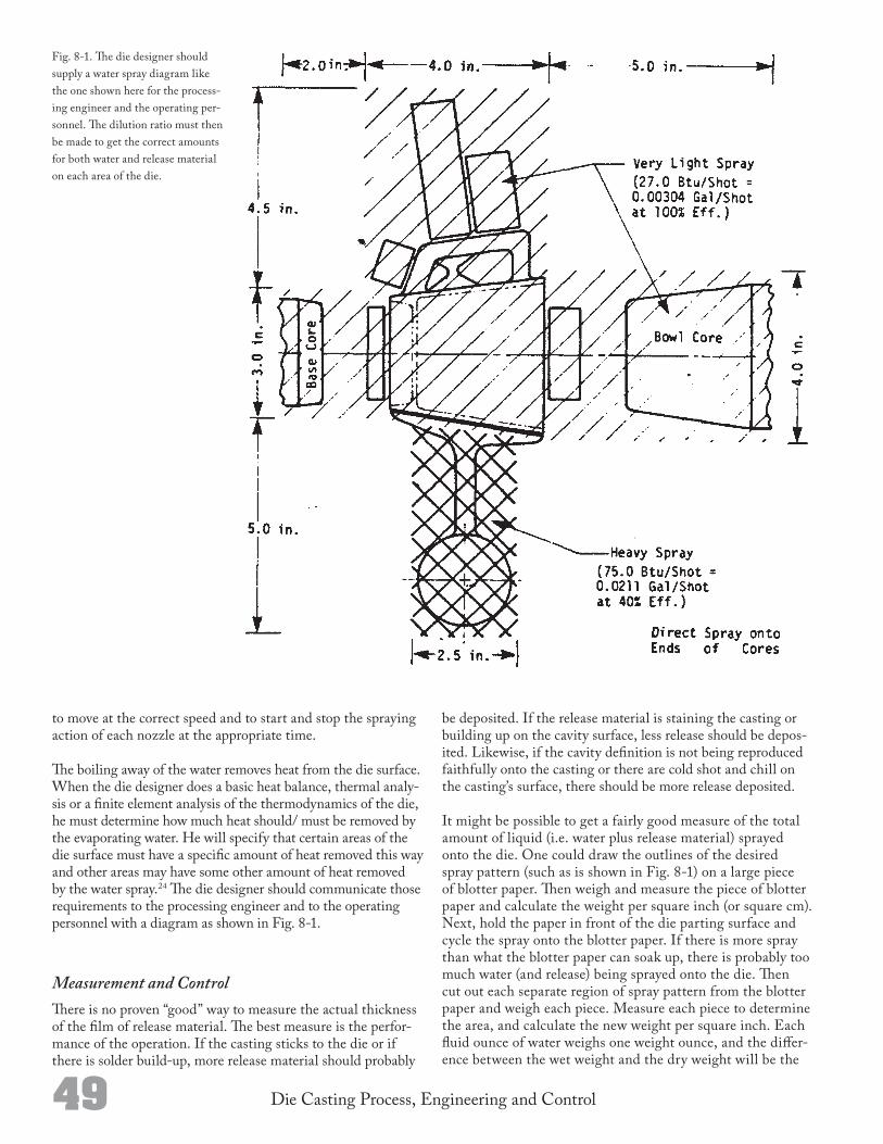
49 Die Casting Process, Engineering and Control

Fig. 8­1. The die designer should supply a water spray diagram like the one shown here for the process­ing engineer and the operating per­sonnel. The dilution ratio must then be made to get the correct amounts for both water and release material on each area of the die.

to move at the correct speed and to start and stop the spraying action of each nozzle at the appropriate time.

The boiling away of the water removes heat from the die surface. When the die designer does a basic heat balance, thermal analy­sis or a finite element analysis of the thermodynamics of the die, he must determine how much heat should/ must be removed by the evaporating water. He will specify that certain areas of the die surface must have a specific amount of heat removed this way and other areas may have some other amount of heat removed by the water spray.24 The die designer should communicate those requirements to the processing engineer and to the operating personnel with a diagram as shown in Fig. 8­1.

Measurement and ControlThere is no proven “good” way to measure the actual thickness of the film of release material. The best measure is the perfor­mance of the operation. If the casting sticks to the die or if there is solder build­up, more release material should probably

be deposited. If the release material is staining the casting or building up on the cavity surface, less release should be depos­ited. Likewise, if the cavity definition is not being reproduced faithfully onto the casting or there are cold shot and chill on the casting’s surface, there should be more release deposited.

It might be possible to get a fairly good measure of the total amount of liquid (i.e. water plus release material) sprayed onto the die. One could draw the outlines of the desired spray pattern (such as is shown in Fig. 8­1) on a large piece of blotter paper. Then weigh and measure the piece of blotter paper and calculate the weight per square inch (or square cm). Next, hold the paper in front of the die parting surface and cycle the spray onto the blotter paper. If there is more spray than what the blotter paper can soak up, there is probably too much water (and release) being sprayed onto the die. Then cut out each separate region of spray pattern from the blotter paper and weigh each piece. Measure each piece to determine the area, and calculate the new weight per square inch. Each fluid ounce of water weighs one weight ounce, and the differ­ence between the wet weight and the dry weight will be the

50Die Casting Process, Engineering and Control

amount of liquid absorbed by the blotter paper. The weight can be compared to the desired amount of spray and the nozzles and/or spray time adjusted accordingly.

As the amount of release is changed to adjust for the casting conditions, it must be remembered that the cooling effect is also changed because different amounts of water are sprayed onto the die. The interdependence of cooling and release is quite unfortunate since both are variables that the process is highly sensitive to, but quite possibly in different ways.

The dilution ratio of water to actual release material is established by Eq. 8-1.

Dilution ratio = Volume of water/Volume of release (8-1)

So, if 1 gallon of release is mixed into 25 gallons of water, the dilution ratio is 25.

Most release materials are already mixed with water when received from the supplier. The mixture ratio of the material “as received” must then be taken into account before the material is actually diluted. The supplier of the release material can best advise as to the best dilution ratio for each application of his product.

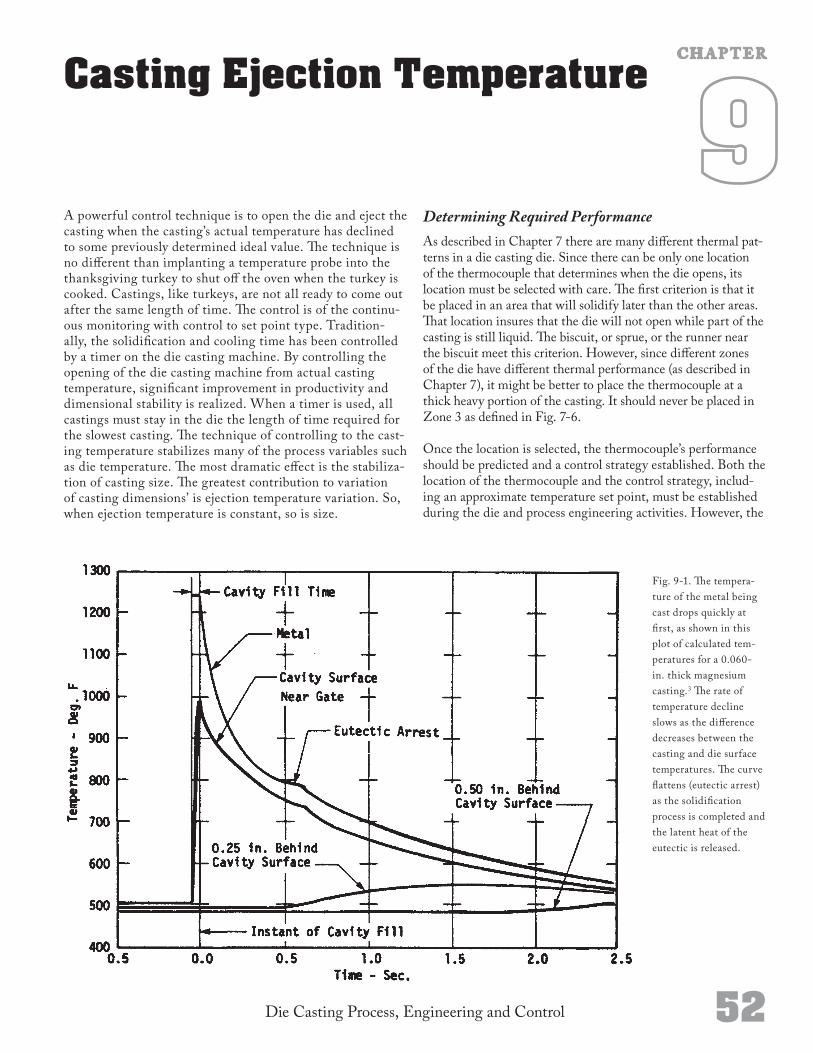
Die Casting Process, Engineering and Control 52

A powerful control technique is to open the die and eject the casting when the casting’s actual temperature has declined to some previously determined ideal value. The technique is no different than implanting a temperature probe into the thanksgiving turkey to shut off the oven when the turkey is cooked. Castings, like turkeys, are not all ready to come out after the same length of time. The control is of the continu­ous monitoring with control to set point type. Tradition­ally, the solidification and cooling time has been controlled by a timer on the die casting machine. By controlling the opening of the die casting machine from actual casting temperature, significant improvement in productivity and dimensional stability is realized. When a timer is used, all castings must stay in the die the length of time required for the slowest casting. The technique of controlling to the cast­ing temperature stabilizes many of the process variables such as die temperature. The most dramatic effect is the stabiliza­tion of casting size. The greatest contribution to variation of casting dimensions’ is ejection temperature variation. So, when ejection temperature is constant, so is size.

Casting Ejection Temperature

Fig. 9­1. The tempera­ture of the metal being cast drops quickly at first, as shown in this plot of calculated tem­peratures for a 0.060­in. thick magnesium casting.3 The rate of temperature decline slows as the difference decreases between the casting and die surface temperatures. The curve flattens (eutectic arrest) as the solidification process is completed and the latent heat of the eutectic is released.

C H A P T E R

Determining Required PerformanceAs described in Chapter 7 there are many different thermal pat­terns in a die casting die. Since there can be only one location of the thermocouple that determines when the die opens, its location must be selected with care. The first criterion is that it be placed in an area that will solidify later than the other areas. That location insures that the die will not open while part of the casting is still liquid. The biscuit, or sprue, or the runner near the biscuit meet this criterion. However, since different zones of the die have different thermal performance (as described in Chapter 7), it might be better to place the thermocouple at a thick heavy portion of the casting. It should never be placed in Zone 3 as defined in Fig. 7­6.

Once the location is selected, the thermocouple’s performance should be predicted and a control strategy established. Both the location of the thermocouple and the control strategy, includ­ing an approximate temperature set point, must be established during the die and process engineering activities. However, the

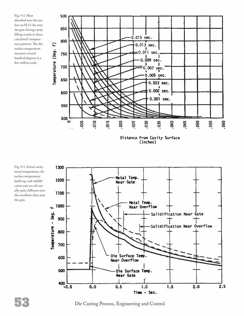
53 Die Casting Process, Engineering and Control

Fig. 9­2. Heat absorbed into the sur­face an H­13 die near the gate during cavity filling results in these calculated3 tempera­ture patterns. The die surface temperature increases several hundred degrees is a few milliseconds.

Fig. 9­3. Initial cavity metal temperature, die surface temperature build­up, and solidifi­cation rate are all usu­ally quite different near the overflows than near the gate.

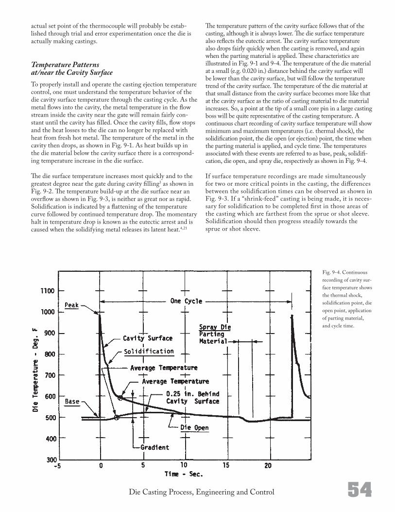
54Die Casting Process, Engineering and Control

Fig. 9­4. Continuous recording of cavity sur­face temperature shows the thermal shock, solidification point, die open point, application of parting material, and cycle time.

actual set point of the thermocouple will probably be estab­lished through trial and error experimentation once the die is actually making castings.

Temperature Patterns at/near the Cavity SurfaceTo properly install and operate the casting ejection temperature control, one must understand the temperature behavior of the die cavity surface temperature through the casting cycle. As the metal flows into the cavity, the metal temperature in the flow stream inside the cavity near the gate will remain fairly con­stant until the cavity has filled. Once the cavity fills, flow stops and the heat losses to the die can no longer be replaced with heat from fresh hot metal. The temperature of the metal in the cavity then drops, as shown in Fig. 9­1. As heat builds up in the die material below the cavity surface there is a correspond­ing temperature increase in the die surface.

The die surface temperature increases most quickly and to the greatest degree near the gate during cavity filling3 as shown in Fig. 9­2. The temperature build­up at the die surface near an overflow as shown in Fig. 9­3, is neither as great nor as rapid. Solidification is indicated by a flattening of the temperature curve followed by continued temperature drop. The momentary halt in temperature drop is known as the eutectic arrest and is caused when the solidifying metal releases its latent heat.4,21

The temperature pattern of the cavity surface follows that of the casting, although it is always lower. The die surface temperature also reflects the eutectic arrest. The cavity surface temperature also drops fairly quickly when the casting is removed, and again when the parting material is applied. These characteristics are illustrated in Fig. 9­1 and 9­4. The temperature of the die material at a small (e.g. 0.020 in.) distance behind the cavity surface will be lower than the cavity surface, but will follow the temperature trend of the cavity surface. The temperature of the die material at that small distance from the cavity surface becomes more like that at the cavity surface as the ratio of casting material to die material increases. So, a point at the tip of a small core pin in a large casting boss will be quite representative of the casting temperature. A continuous chart recording of cavity surface temperature will show minimum and maximum temperatures (i.e. thermal shock), the solidification point, the die open (or ejection) point, the time when the parting material is applied, and cycle time. The temperatures associated with these events are referred to as base, peak, solidifi­cation, die open, and spray die, respectively as shown in Fig. 9­4.

If surface temperature recordings are made simultaneously for two or more critical points in the casting, the differences between the solidification times can be observed as shown in Fig. 9­3. If a “shrink­feed” casting is being made, it is neces­sary for solidification to be completed first in those areas of the casting which are farthest from the sprue or shot sleeve. Solidification should then progress steadily towards the sprue or shot sleeve.

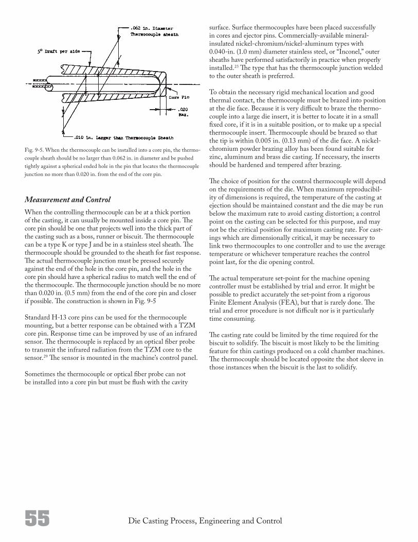
55 Die Casting Process, Engineering and Control

Fig. 9­5. When the thermocouple can be installed into a core pin, the thermo­couple sheath should be no larger than 0.062 in. in diameter and be pushed tightly against a spherical ended hole in the pin that locates the thermocouple junction no more than 0.020 in. from the end of the core pin.

Measurement and ControlWhen the controlling thermocouple can be at a thick portion of the casting, it can usually be mounted inside a core pin. The core pin should be one that projects well into the thick part of the casting such as a boss, runner or biscuit. The thermocouple can be a type K or type J and be in a stainless steel sheath. The thermocouple should be grounded to the sheath for fast response. The actual thermocouple junction must be pressed securely against the end of the hole in the core pin, and the hole in the core pin should have a spherical radius to match well the end of the thermocouple. The thermocouple junction should be no more than 0.020 in. (0.5 mm) from the end of the core pin and closer if possible. The construction is shown in Fig. 9­5

Standard H­13 core pins can be used for the thermocouple mounting, but a better response can be obtained with a TZM core pin. Response time can be improved by use of an infrared sensor. The thermocouple is replaced by an optical fiber probe to transmit the infrared radiation from the TZM core to the sensor.29 The sensor is mounted in the machine’s control panel.

Sometimes the thermocouple or optical fiber probe can not be installed into a core pin but must be flush with the cavity

surface. Surface thermocouples have been placed successfully in cores and ejector pins. Commercially­available mineral­insulated nickel­chromium/nickel­aluminum types with 0.040­in. (1.0 mm) diameter stainless steel, or “Inconel,” outer sheaths have performed satisfactorily in practice when properly installed.23 The type that has the thermocouple junction welded to the outer sheath is preferred.

To obtain the necessary rigid mechanical location and good thermal contact, the thermocouple must be brazed into position at the die face. Because it is very difficult to braze the thermo­couple into a large die insert, it is better to locate it in a small fixed core, if it is in a suitable position, or to make up a special thermocouple insert. Thermocouple should be brazed so that the tip is within 0.005 in. (0.13 mm) of the die face. A nickel­chromium powder brazing alloy has been found suitable for zinc, aluminum and brass die casting. If necessary, the inserts should be hardened and tempered after brazing.

The choice of position for the control thermocouple will depend on the requirements of the die. When maximum reproducibil­ity of dimensions is required, the temperature of the casting at ejection should be maintained constant and the die may be run below the maximum rate to avoid casting distortion; a control point on the casting can be selected for this purpose, and may not be the critical position for maximum casting rate. For cast­ings which are dimensionally critical, it may be necessary to link two thermocouples to one controller and to use the average temperature or whichever temperature reaches the control point last, for the die opening control.

The actual temperature set­point for the machine opening controller must be established by trial and error. It might be possible to predict accurately the set­point from a rigorous Finite Element Analysis (FEA), but that is rarely done. The trial and error procedure is not difficult nor is it particularly time consuming.

The casting rate could be limited by the time required for the biscuit to solidify. The biscuit is most likely to be the limiting feature for thin castings produced on a cold chamber machines. The thermocouple should be located opposite the shot sleeve in those instances when the biscuit is the last to solidify.

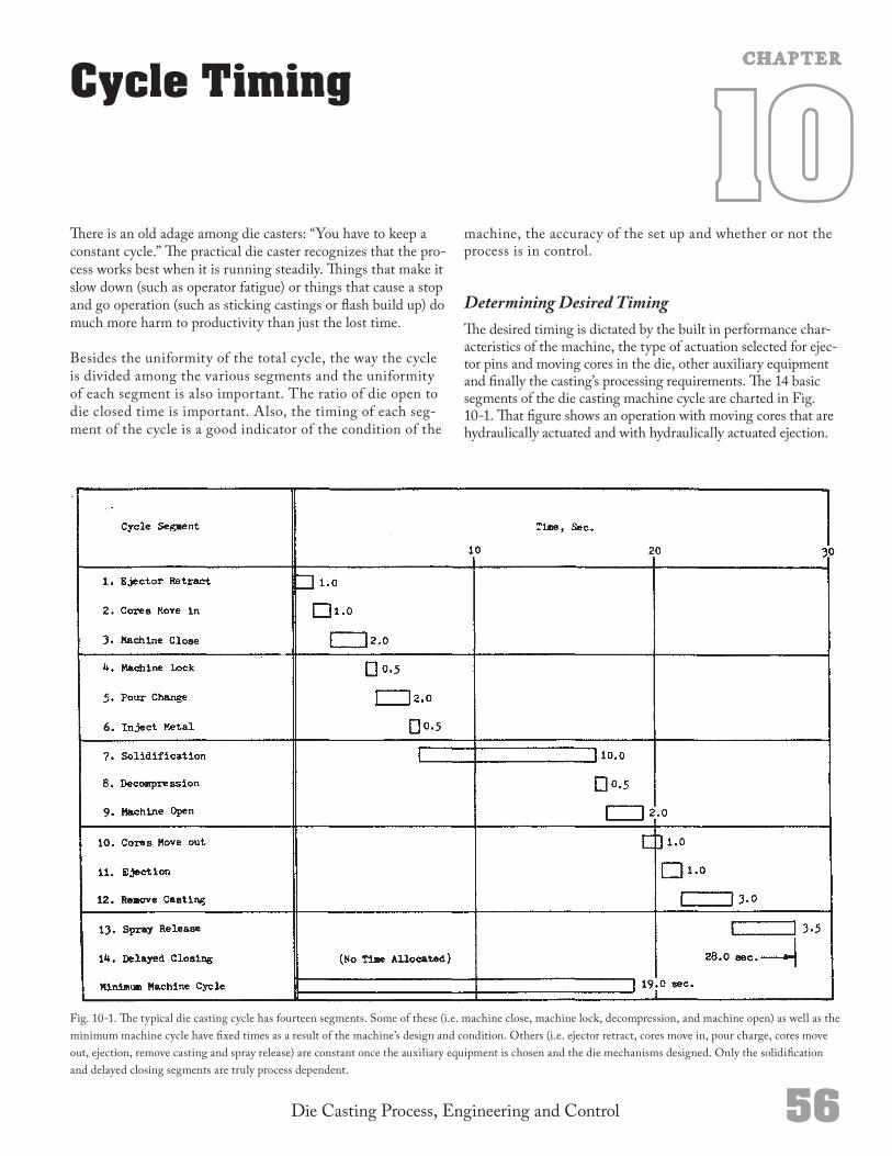
Die Casting Process, Engineering and Control 56

There is an old adage among die casters: “You have to keep a constant cycle.” The practical die caster recognizes that the pro­cess works best when it is running steadily. Things that make it slow down (such as operator fatigue) or things that cause a stop and go operation (such as sticking castings or flash build up) do much more harm to productivity than just the lost time.

Besides the uniformity of the total cycle, the way the cycle is divided among the various segments and the uniformity of each segment is also important. The ratio of die open to die closed time is important. Also, the timing of each seg­ment of the cycle is a good indicator of the condition of the

Cycle Timing

Fig. 10­1. The typical die casting cycle has fourteen segments. Some of these (i.e. machine close, machine lock, decompression, and machine open) as well as the minimum machine cycle have fixed times as a result of the machine’s design and condition. Others (i.e. ejector retract, cores move in, pour charge, cores move out, ejection, remove casting and spray release) are constant once the auxiliary equipment is chosen and the die mechanisms designed. Only the solidification and delayed closing segments are truly process dependent.

C H A P T E R

machine, the accuracy of the set up and whether or not the process is in control.

Determining Desired TimingThe desired timing is dictated by the built in performance char­acteristics of the machine, the type of actuation selected for ejec­tor pins and moving cores in the die, other auxiliary equipment and finally the casting’s processing requirements. The 14 basic segments of the die casting machine cycle are charted in Fig. 10­1. That figure shows an operation with moving cores that are hydraulically actuated and with hydraulically actuated ejection.

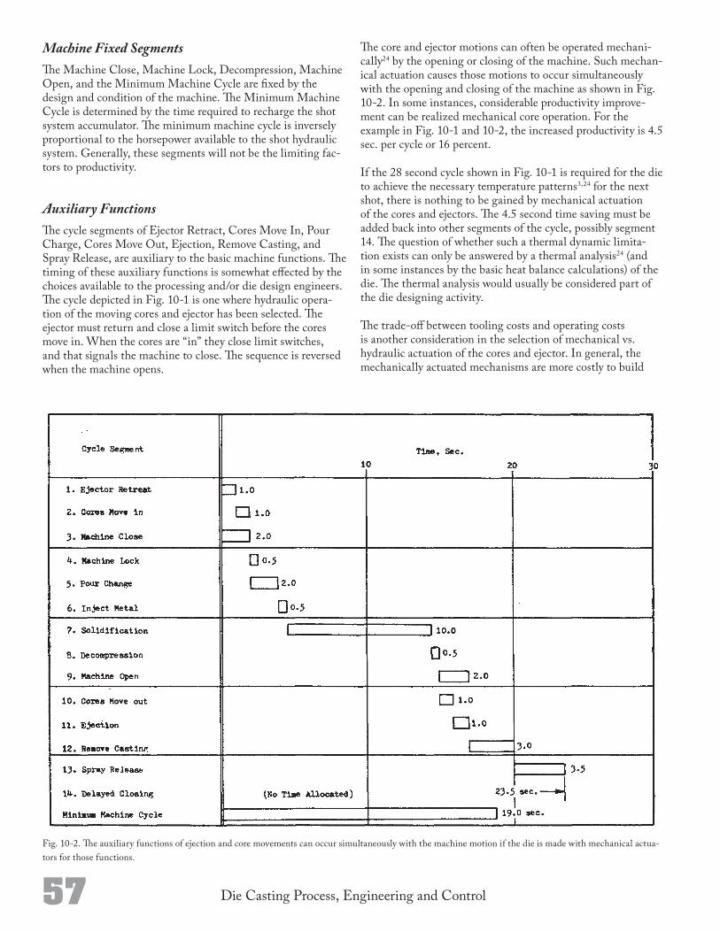
57 Die Casting Process, Engineering and Control

Fig. 10­2. The auxiliary functions of ejection and core movements can occur simultaneously with the machine motion if the die is made with mechanical actua­tors for those functions.

Machine Fixed SegmentsThe Machine Close, Machine Lock, Decompression, Machine Open, and the Minimum Machine Cycle are fixed by the design and condition of the machine. The Minimum Machine Cycle is determined by the time required to recharge the shot system accumulator. The minimum machine cycle is inversely proportional to the horsepower available to the shot hydraulic system. Generally, these segments will not be the limiting fac­tors to productivity.

Auxiliary FunctionsThe cycle segments of Ejector Retract, Cores Move In, Pour Charge, Cores Move Out, Ejection, Remove Casting, and Spray Release, are auxiliary to the basic machine functions. The timing of these auxiliary functions is somewhat effected by the choices available to the processing and/or die design engineers. The cycle depicted in Fig. 10­1 is one where hydraulic opera­tion of the moving cores and ejector has been selected. The ejector must return and close a limit switch before the cores move in. When the cores are “in” they close limit switches, and that signals the machine to close. The sequence is reversed when the machine opens.

The core and ejector motions can often be operated mechani­cally24 by the opening or closing of the machine. Such mechan­ical actuation causes those motions to occur simultaneously with the opening and closing of the machine as shown in Fig. 10­2. In some instances, considerable productivity improve­ment can be realized mechanical core operation. For the example in Fig. 10­1 and 10­2, the increased productivity is 4.5 sec. per cycle or 16 percent.

If the 28 second cycle shown in Fig. 10­1 is required for the die to achieve the necessary temperature patterns3,24 for the next shot, there is nothing to be gained by mechanical actuation of the cores and ejectors. The 4.5 second time saving must be added back into other segments of the cycle, possibly segment 14. The question of whether such a thermal dynamic limita­tion exists can only be answered by a thermal analysis24 (and in some instances by the basic heat balance calculations) of the die. The thermal analysis would usually be considered part of the die designing activity.

The trade­off between tooling costs and operating costs is another consideration in the selection of mechanical vs. hydraulic actuation of the cores and ejector. In general, the mechanically actuated mechanisms are more costly to build

58Die Casting Process, Engineering and Control

into the die. The higher costs are especially the case for large dies and large cores. Being part of the die, these costs are “up front” money. From a business standpoint, it is usually best to delay expenditures. So, the extra tooling costs must be adjusted for the time value of money (equivalent interest earning power) and amortized into all the parts to be made during the life of the product. If the resulting increased piece part cost exceeds the operating costs of the extra 16 percent of cycle time, the mechanical system should not be used.

The Pour Charge (i.e. ladle), Remove Casting, and Spray Release segments are also auxiliary functions, but are some­what different than the die actuations. These relate to auxiliary equipment associated with the die casting machine rather than the die. These time segments can only be changed by replacing or updating that equipment. One must make sure that if the equipment is programmable that it is not poorly programmed and is therefore operating more slowly than necessary.

Inject MetalThe cycle segment of injecting the molten metal is process dependent,2,13 but, is such a small part of the total that it is very seldom a consideration in the sense of the processing variation considered in this chaper. The timing within the segment is critical to the process, but those considerations are discussed in Chapter 5. Technically, the intensification build up time is part of this segment although it overlaps solidification.

Process Dependent SegmentsThe solidification and Delayed Closing segments are the only parts of the cycle that are truly process dependent. The solidi­fication time must be long enough to solidify and adequately cool all parts of the cast shot. The principle effect of increasing solidification time is to decrease casting ejection temperature. The ramifications of casting ejection temperature are discussed in Chapter 9. For each size of die casting machine, there is a minimum solidification time for the biscuit or sprue. In many instances the biscuit or sprue governs the solidification time. The casting could be removed sooner, if sprue or biscuit were solidified so the machine could be opened.

The delayed closing segment is almost always hidden and its existence denied. The function of the delayed closing is to provide sufficient total cycle time for the cooling water circu­lating through the die to remove the necessary amount of heat before the next shot. However, if it is put into the cycle as a true delay, the machine and operator will appear to be under­utilized and managers will try to get the operation speeded up

on the basis of time and motion concepts. Anyone that sets up a manufacturing operation with obvious delays is always open to criticism. So, the time is sometimes added into the cycle by adding time for spraying release. It is sometimes provided, at least in part, by having sequenced rather than simultaneous auxiliary functions. The net result is the same. The total cycle accommodates the thermodynamics of the die. By putting extra time into the spraying of the release material or the die closed time, additional die cooling is achieved which might work to shorten the cycle time, but more likely just reduces die temperature and hence die life.

Sometimes the required cycle time is achieved by adding the time to the solidification segment instead of having delayed closing time. That segment is always considered to be pure processing time (and therefore required) and not likely to draw criticism. This ploy may not work if dimensional tolerances are critical on the casting. The actual size of the casting is strongly dependent upon its ejection temperature1 (see Chapter 9), and the ejection temperature is determined, in part, by the time the casting is in the die. So, solidification time and total cycle time must be considered separately to achieve some performance requirements such as casting size.

Actual Performance MeasurementThe actual timing of the machine cycle segments can be mea­sured directly from the machine’s programmable logic control­ler (PLC). Each segment begins with some type of electrical control signal. A limit switch must close or open, a timer times out, or power is directed to a solenoid. If these are not conve­nient, the PLC can be programmed to output specific signals for the purpose of measurement.

The PLC signals can be processed through a resistor panel to reduce the voltage as required and then recorded on a chart recorder or read directly by a micro processor. A micro proces­sor can be programmed to display the segment timing much like the bar charts shown in Figs. 10­1 and 10­2. The micro processor could even highlight any segment not performing to a pre­established time duration.

A micro processor could monitor the operation continuously and activate an alarm if any segment exceeded its designed limits. Then a technician could review the displayed chart of all segments as well as other performance measurements to determine corrective action. The micro processor could have stored in memory the original performance characteristics of the machine. These data could be an important preventive maintenance tool.

Die Casting Process, Engineering and Control 61

Generally the mechanical parts of the die are not considered to be processing variables. Nevertheless some parts of the die are subject to wear and/or breakage and can therefore put the process “out of control”. When a part breaks, it is a catastrophic event. As wear occurs the process exhibits continuous drift. Both of these characteristics were described in the Introduc­tion, Chapter 1, of this book. Continuous drift is the behavior that is ideally suited to statistical process control (SPC) meth­ods, and that is the condition discussed in this chapter.

Characteristics of Die Cavity WearDie cavities wear slowly. Usually it takes weeks or months to achieve a distinguishable amount of wear. Wear on the cavity surface is caused by erosion/cavitation, heat checking, and soldering. Dimensions of features created by two different die members (such as dimensions that cross the parting line) can change because of wear in the mechanical surfaces such as gibs or leader pins that align the die members.

Erosion and/or cavitation occurs where gas bubbles entrained in the molten metal flow collapse with great violence at the instant of cavity filling.

Heat checking is the most common form of cavity wear. The thermal shock of the injected metal deforms the steel at the surface of the cavity. The repeated deformations fatigue the steel and it develops hair line cracks. At first the resulting cracks form a crazing of the surface. The cracks can either grow into visible crazing, or can let the small pieces of die steel between them be broken away. If the sprayed on release is washed out of the cracks during cavity filling, the molten metal can fill them and cause the casting to stick to the die. When the casting is ejected off such surfaces, the cast metal may shear away from the cavity leaving an obvious trace of cast metal on the cavity surface. This condition is usually identified as soldering although heat checking is the root cause. (True soldering is any time the cast metal establishes a metallurgical bond to the cavity surface. The casting is sheared or torn off the resulting intermetallic layer as it is ejected leaving a rough layer of cast metal on the cavity surface.)

Soldering and heat checking do not necessarily change the surface dimensionally. Soldering can result in a build up on the cavity surface that can change a casting’s dimension. The normal cause of change is the polishing that is done to the cavity surface to remove the heat checked or soldered condition. Sometimes cavities must be polished daily for such conditions.

Mechanical Die SystemC H A P T E R

If the die could be cooled periodically to room temperature and measured, changes in dimensions of cavity features could be assessed quite straight forwardly. However, it is usually more prac­tical for many reasons to measure the castings and deduce the con­dition of the die from those measurements. Unfortunately, a single measurement of a single casting may not accurately reveal the true condition of the die. Statistical methods are often required.

When a die casting die is operating under normal conditions and the cavity is not deteriorating, there is considerable variation of the casting dimensions. Those short term dimensional variations will tend to mask the long term deterioration due to wear. The short term process induced dimensional variations are of four types:

1) Linear

2) Parting Line (Blow)3) Shift/Match4) Warpage

The specific type of variation is determined by how the feature of the casting is formed between the members of the die. The mathematical relationships between the dimensional variations, die constructions and processing variables is developed fully in the NADCA Textbook Dimensional Repeatability and the associated NADCA course. A statistical process control (SPC) X and R chart as described in Chapter 3 would quantify those short term varia­tions. Such a control chart would look much like Fig. 3­1 except the vertical scales would be dimensions instead of temperatures.

The short term dimensional variations would have periods between peaks of a few hours, and in some instances several minutes. Samples should be collected and measured hourly. Within a few days, control limits could be established and an effective SPC system put into operation.

Establishing Desired ConditionsThe goal is to avoid having any dimension get outside of the part print tolerance due to die deterioration. So, SPC X and R control charts should be set up for all critical dimensions plus non­criti­cal dimensions that are expected to be (or subsequently found to be) subject to wear. Initially, such charts are not likely to show the long term drift of wear. Instead, they will describe the effects of the more short term processing variables such as die tempera­ture. Within a week of steady operation the control limits can be established and the X and R chart will be a working tool. Then is when the engineer should start watching for wear.

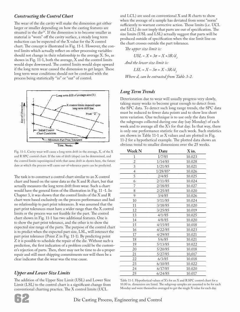
62 Die Casting Process, Engineering and Control

Constructing the Control ChartThe wear of the die cavity will make the dimension get either larger or smaller depending on how the casting features are situated in the die24. If the dimension is to become smaller as material is “worn” off the cavity surface, a steady long term reduction can be expected of the X value for the X control chart. The concept is illustrated in Fig. 11­1. However, the con­trol limits which actually reflect on other processing variables should not change in their relationship to the average X. So, as shown in Fig. 11­1, both the average, X and the control limits would slope downward. The control limits would slope upward if the long term wear caused the dimension to get larger. These long term wear conditions should not be confused with the process being statistically “in” or “out” of control.

Fig. 11­1. Cavity wear will cause a long term drift in the average, X, of the X and R SPC control chart. If the rate of drift (slope) can be determined, and the control limits superimposed with that same drift as shown here, the future date at which the process will cause out­of­tolerance parts can be predicted.

The task is to construct a control chart similar to an X control chart and based on the same data as the X and R chart, but that actually measures the long term drift from wear. Such a chart would have the general form of the illustration in Fig. 11 ­1. In Chapter 3, it was shown that the control limits of the X and R chart were based exclusively on the process performance and had no relationship to part print tolerances. It was assumed that the part print tolerances must have a wider range than the X control limits or the process was not feasible for the part. The control chart shown in Fig. 11­1 has two additional features. One is to show the part print tolerance, and the other is to show the expected size range of the parts. The purpose of the control chart is to predict when the expected part size, LSL, will intersect the part print tolerance (Point Z in Fig. 11­1). By predicting point Z it is possible to schedule the repair of the die. Without such­a prediction, the first indication of a problem could be the custom­er’s rejection of parts. Then, there may not be time to do a proper repair and still meet shipping commitments nor will there be a clear indicator that die wear was the true cause.

Upper and Lower Size LimitsThe addition of the Upper Size Limit (USL) and Lower Size Limit (LSL) to the control chart is a significant change from conventional charting practice. The X control limits (UCL

and LCL) are used on conventional X and R charts to show when the average of a sample has deviated from some “norm” sufficiently to warrant corrective action. Those limits (i.e. UCL and LCL) do not imply that parts are out of specification. The size limits (USL and LSL) actually suggest that parts will be produced outside of specification when the size limit line on the chart crosses outside the part tolerance.

The upper size limit is: USL = X + 3σ = X +3R/d2

And the lower size limit is: LSL = X – 3σ = X -3R/d2

Where d, can be extracted from Table 3-2.

Long Term TrendsDeterioration due to wear will usually progress very slowly, taking many weeks to become great enough to detect from the SPC data. To detect such long range trends, the SPC data must be reduced to fewer data points and to show less short term variation. One technique is to use only the data from the subgroups collected during one day (say Monday) of each week and to average all the X’s for that day. In that way, there is only one performance statistic for each week. Such statistics are shown in Table 11­1 as X values and are plotted in Fig. 11­2 for a hypothetical example. The plotted data shows an obvious trend to smaller dimensions over the 25 weeks.

Week N Date X in.1 I/7/85 10.0232 1/14/85 10.0283 1/21/85 10.0214 1/28/85* 10.0265 2/4/85 10.0256 2/11/85 10.0247 2/18/85 10.0278 2/25/85 10.0209 3/4/85 10.02610 3/11/85 10.02411 3/18/85 10.02012 3/25/85 10.01913 4/1/85 10.02514 4/8/85 10.02015 4/15/85 10.01816 4/22/85 10.02317 4/29/85 10.02118 5/6/85 10.02119 5/13/85 10.02220 5/20/85 10.01821 5/27/85 10,01722 6/3/85 10.01823 6/10/85 10.02224 6/17/85 10.02025 6/24/85 10.017

Table 11­1. Hypothetical values of X’s for an X and R SPC control chart for a 10.00 in. dimension are listed. The subgroup samples are assumed to be for each Monday and were themselves averaged to get the single X value for each day.

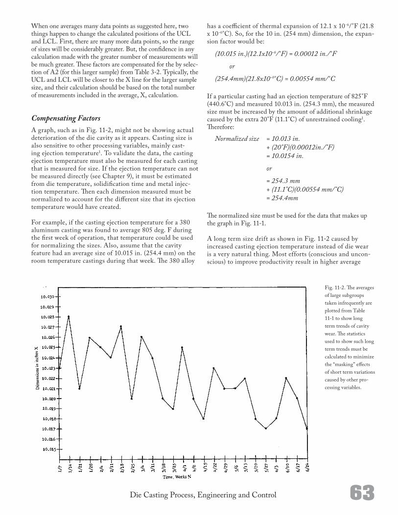
63Die Casting Process, Engineering and Control

Fig. 11­2. The averages of large subgroups taken infrequently are plotted from Table 11­1 to show long term trends of cavity wear. The statistics used to show such long term trends must be calculated to minimize the “masking” effects of short term variations caused by other pro­cessing variables.

When one averages many data points as suggested here, two things happen to change the calculated positions of the UCL and LCL. First, there are many more data points, so the range of sizes will be considerably greater. But, the confidence in any calculation made with the greater number of measurements will be much greater. These factors are compensated for the by selec­tion of A2 (for this larger sample) from Table 3­2. Typically, the UCL and LCL will be closer to the X line for the larger sample size, and their calculation should be based on the total number of measurements included in the average, X, calculation.

Compensating FactorsA graph, such as in Fig. 11­2, might not be showing actual deterioration of the die cavity as it appears. Casting size is also sensitive to other processing variables, mainly cast­ing ejection temperature1. To validate the data, the casting ejection temperature must also be measured for each casting that is measured for size. If the ejection temperature can not be measured directly (see Chapter 9), it must be estimated from die temperature, solidification time and metal injec­tion temperature. Then each dimension measured must be normalized to account for the different size that its ejection temperature would have created.

For example, if the casting ejection temperature for a 380 aluminum casting was found to average 805 deg. F during the first week of operation, that temperature could be used for normalizing the sizes. Also, assume that the cavity feature had an average size of 10.015 in. (254.4 mm) on the room temperature castings during that week. The 380 alloy

has a coefficient of thermal expansion of 12.1 x 10­6/°F (21.8 x 10­6°C). So, for the 10 in. (254 mm) dimension, the expan­sion factor would be:

(10.015 in.)(12.1x10-6/ °F) = 0.00012 in./ °F

or

(254.4mm)(21.8x10-6°C) = 0.00554 mm/ °C

If a particular casting had an ejection temperature of 825°F (440.6°C) and measured 10.013 in. (254.3 mm), the measured size must be increased by the amount of additional shrinkage caused by the extra 20°F (11.1°C) of unrestrained cooling1. Therefore:

Normalized size = 10.013 in. + (20°F)(0.00012in./°F) = 10.0154 in.

or

= 254.3 mm + (11.1°C)(0.00554 mm/°C) = 254.4mm

The normalized size must be used for the data that makes up the graph in Fig. 11­1.

A long term size drift as shown in Fig. 11­2 caused by increased casting ejection temperature instead of die wear is a very natural thing. Most efforts (conscious and uncon­scious) to improve productivity result in higher average

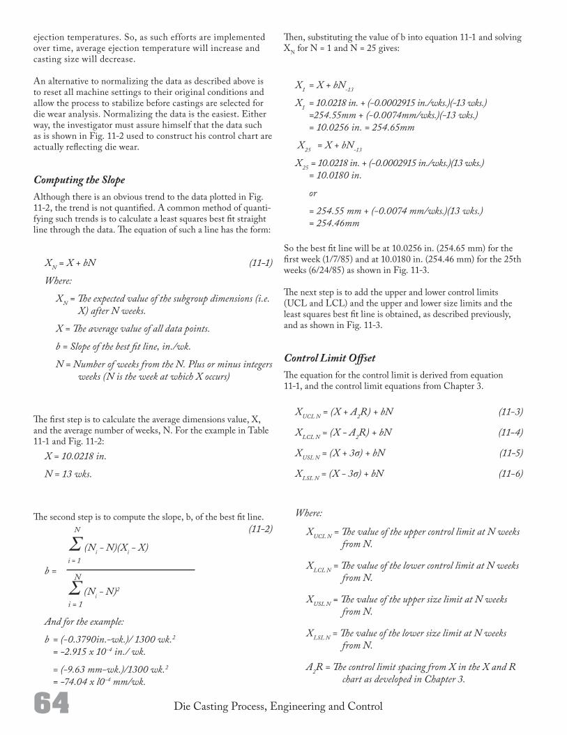
64 Die Casting Process, Engineering and Control

ejection temperatures. So, as such efforts are implemented over time, average ejection temperature will increase and casting size will decrease.

An alternative to normalizing the data as described above is to reset all machine settings to their original conditions and allow the process to stabilize before castings are selected for die wear analysis. Normalizing the data is the easiest. Either way, the investigator must assure himself that the data such as is shown in Fig. 11­2 used to construct his control chart are actually reflecting die wear.

Computing the SlopeAlthough there is an obvious trend to the data plotted in Fig. 11­2, the trend is not quantified. A common method of quanti­fying such trends is to calculate a least squares best fit straight line through the data. The equation of such a line has the form:

XN = X + bN (11-1)

Where:

XN = The expected value of the subgroup dimensions (i.e. X) after N weeks.

X = The average value of all data points.

b = Slope of the best fit line, in./wk.

N = Number of weeks from the N. Plus or minus integers weeks (N is the week at which X occurs)

The first step is to calculate the average dimensions value, X, and the average number of weeks, N. For the example in Table 11­1 and Fig. 11­2:

X = 10.0218 in.

N = 13 wks.

The second step is to compute the slope, b, of the best fit line. N (11-2)

Σ (Ni - N)(Xi - X) i = 1b = N Σ (Ni - N)2 i = 1

And for the example:

b = (-0.3790in.-wk.)/ 1300 wk.2 = -2.915 x 10-4 in./ wk.

= (-9.63 mm-wk.)/1300 wk.2 = -74.04 x l0-4 mm/wk.

Then, substituting the value of b into equation 11­1 and solving XN for N = 1 and N = 25 gives:

X1 = X + bN-13

X1 = 10.0218 in. + (-0.0002915 in./wks.)(-13 wks.) =254.55mm + (-0.0074mm/wks.)(-13 wks.) = 10.0256 in. = 254.65mm

X25 = X + bN-13

X25 = 10.0218 in. + (-0.0002915 in./wks.)(13 wks.) = 10.0180 in.

or

= 254.55 mm + (-0.0074 mm/wks.)(13 wks.) = 254.46mm

So the best fit line will be at 10.0256 in. (254.65 mm) for the first week (1/7/85) and at 10.0180 in. (254.46 mm) for the 25th weeks (6/24/85) as shown in Fig. 11­3.

The next step is to add the upper and lower control limits (UCL and LCL) and the upper and lower size limits and the least squares best fit line is obtained, as described previously, and as shown in Fig. 11­3.

Control Limit OffsetThe equation for the control limit is derived from equation 11­1, and the control limit equations from Chapter 3.

XUCL N = (X + A2R) + bN (11-3)

XLCL N = (X - A2R) + bN (11-4)

XUSL N = (X + 3σ) + bN (11-5)

XLSL N = (X - 3σ) + bN (11-6)

Where:

XUCL N = The value of the upper control limit at N weeks from N.

XLCL N = The value of the lower control limit at N weeks from N.

XUSL N = The value of the upper size limit at N weeks from N.

XLSL N = The value of the lower size limit at N weeks from N.

A2R = The control limit spacing from X in the X and R chart as developed in Chapter 3.

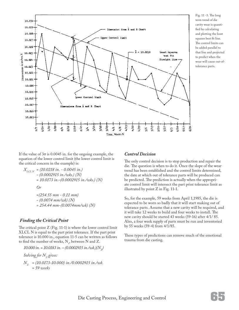
65Die Casting Process, Engineering and Control

Fig. 11 ­3. The long term trend of die cavity wear is quanti­fied by calculating and plotting the least squares best fit line. The control limits can be added parallel to that line and projected to predict when the wear will cause out­of­tolerance parts.

If the value of 3σ is 0.0045 in. for the ongoing example, the equation of the lower control limit (the lower control limit is the critical concern in the example) is:

XLCL N = (10.0218 in. - 0.0045 in.) - (0.0002915 in./wks.) (N) = 10.0173 in.-(0.0002915 in./wks.) (N)

Or

=(254.55 mm - 0.11 mm) - (0.0074 mm/wk) (N) = 254.44 mm-(0.0074mm/wk) (N)

Finding the Critical PointThe critical point Z (Fig. 11­1) is where the lower control limit XLCL N is equal to the part print tolerance. If the part print tolerance is 10.000 in., equation 11­5 can be written as follows to find the number of weeks, Nz, between N and Z.

10.000 in. = 10.0183 in. – (0.0002915 in./wk.)(NZ)

Solving for NZ gives:

NZ = (10.0173-10.000) in./0.0002915 in./wk. = 59 weeks

Control DecisionThe only control decision is to stop production and repair the die. The question is when to do it. Once the slope of the wear trend has been established and the control limits determined, the date at which out of tolerance parts will be produced can be predicted. The prediction is actually when the appropri­ate control limit will intersect the part print tolerance limit as illustrated by point Z in Fig. 11­1.

So, for the example, 59 weeks from April 1,1985, the die is expected to be worn so badly that it will start making out of tolerance parts. Assume that a new cavity will be required, and it will take 12 weeks to build and four weeks to install. The new cavity should be started 43 weeks (59­16) after 4/1/ 85. Also, a four week supply of parts must be run and inventoried by 55 weeks (59­4) from 4/1/85.

These types of predictions can remove much of the emotional trauma from die casting.

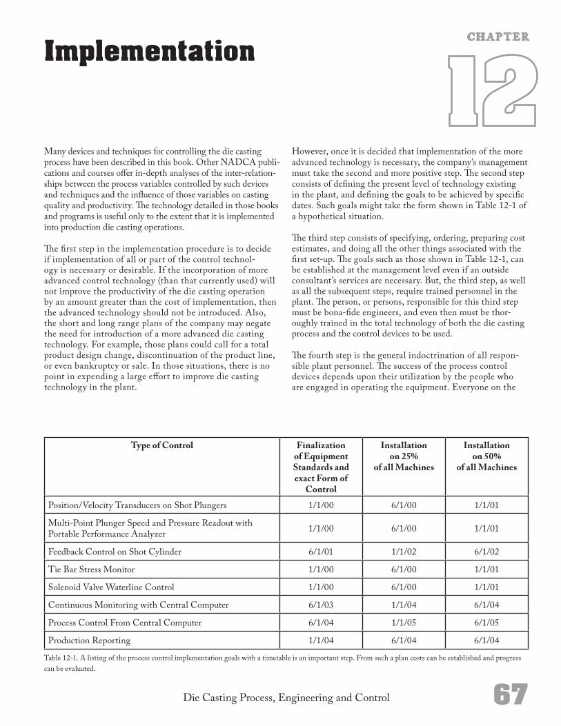
Die Casting Process, Engineering and Control 67

Many devices and techniques for controlling the die casting process have been described in this book. Other NADCA publi­cations and courses offer in­depth analyses of the inter­relation­ships between the process variables controlled by such devices and techniques and the influence of those variables on casting quality and productivity. The technology detailed in those books and programs is useful only to the extent that it is implemented into production die casting operations.

The first step in the implementation procedure is to decide if implementation of all or part of the control technol­ogy is necessary or desirable. If the incorporation of more advanced control technology (than that currently used) will not improve the productivity of the die casting operation by an amount greater than the cost of implementation, then the advanced technology should not be introduced. Also, the short and long range plans of the company may negate the need for introduction of a more advanced die casting technology. For example, those plans could call for a total product design change, discontinuation of the product line, or even bankruptcy or sale. In those situations, there is no point in expending a large effort to improve die casting technology in the plant.

Implementation

Type of Control Finalization of Equipment Standards and exact Form of

Control

Installation on 25%

of all Machines

Installation on 50%

of all Machines

Position/Velocity Transducers on Shot Plungers 1/1/00 6/1/00 1/1/01

Multi­Point Plunger Speed and Pressure Readout with Portable Performance Analyzer 1/1/00 6/1/00 1/1/01

Feedback Control on Shot Cylinder 6/1/01 1/1/02 6/1/02

Tie Bar Stress Monitor 1/1/00 6/1/00 1/1/01

Solenoid Valve Waterline Control 1/1/00 6/1/00 1/1/01

Continuous Monitoring with Central Computer 6/1/03 1/1/04 6/1/04

Process Control From Central Computer 6/1/04 1/1/05 6/1/05

Production Reporting 1/1/04 6/1/04 6/1/04

Table 12­1. A listing of the process control implementation goals with a timetable is an important step. From such a plan costs can be established and progress can be evaluated.

C H A P T E R

However, once it is decided that implementation of the more advanced technology is necessary, the company’s management must take the second and more positive step. The second step consists of defining the present level of technology existing in the plant, and defining the goals to be achieved by specific dates. Such goals might take the form shown in Table 12­1 of a hypothetical situation.

The third step consists of specifying, ordering, preparing cost estimates, and doing all the other things associated with the first set­up. The goals such as those shown in Table 12­1, can be established at the management level even if an outside consultant’s services are necessary. But, the third step, as well as all the subsequent steps, require trained personnel in the plant. The person, or persons, responsible for this third step must be bona­fide engineers, and even then must be thor­oughly trained in the total technology of both the die casting process and the control devices to be used.

The fourth step is the general indoctrination of all respon­sible plant personnel. The success of the process control devices depends upon their utilization by the people who are engaged in operating the equipment. Everyone on the

68 Die Casting Process, Engineering and Control

“team” must be introduced to the equipment, its philosophy, and the details of their specific duties or role.

The fifth step is to evaluate the results of the first phase of installation. These results may indicate that changes should be made to the basic plan, Table 12­1. Also, the experi­ence gained should result in formalization of the exact (and standardized) type, installation, and procedures that are to be used. This step should also include the establishment of information feed­back control systems to insure the continu­ing function of the devices and learned technology.

The final step is to install the devices and incorporate the oper­ating procedures on the die casting machines as planned.

The most difficult problem is the maintenance of a high level of process control. Little by little, one thing after another will slip out of control. The effect of each loss may be imperceptible. But, collectively, and after a period of time, the gains from the process controls will be lost. For this reason, the information systems to get details of daily performance (and evaluation), back to the line foreman and the machine operators, may be more critical than the technology. Standard “labor efficiency” techniques are definitely not adequate to the task.

Process control is an operational philosophy. It includes operating procedures and the general education of the responsible people. Installation of clever instrumentation and “black boxes” is not sufficient.

Die Casting Process, Engineering and Control 70

Many devices and instruments have been described in this book along with the operating principles by which these devices can be used to control the die casting process. The process technology set forth is sufficient for many degrees of control, which may be classified as:

Manual

Periodic Checks

Continuous Display and/or alarm

Computer control

As any particular installation is advanced from one level of control to the next, there will be an improvement in total useable pieces per shift, less scrap, better surface finish, higher dimensional repeatability, and better internal integ­rity of castings. It has been demonstrated30 that die castings can be produced to tolerance ranges of one tenth of those commercially produced. Likewise, tests have shown that corrosion failure risks of chromium­plated zinc die cast­

Process PotentialC H A P T E R

ings can be greatly reduced5 through control of the casting process. And, the control of internal soundness has been the subject of many research projects and papers.

If the critical variables are continuously monitored, potentially defective castings could theoretically be detected before the die is open. By implementing the proper measuring devices and readout or alarm controllers, the “good” castings could be certi­fied to conform to the specifications. The required measure­ments and control decisions would depend on the particular casting and its specifications. The limits of the measured values could not be pre­calculated in all situations. There usually would be a try­out period to establish the exact relationship between casting quality and the process variables.

The magnitude of the process potential for exploiting markets not generally serviced is great. Now, the means is available for extracting the required performance from the process. Together, these two situations present the greatest challenge ever faced by the die casting industry.

73Die Casting Process, Engineering and Control

1. E. A. Herman, Dimensional Repeatability of the Die Casting Process, The Society of Die Casting Engineers, Inc., 1982.

2. P. Thukkarum, H. H. Pokorny, Gating Die Casting Die, The Society of Die Casting Engineers, Inc., 1977.

3. E. A. Herman, Heat Flow in the Die Casting Process, The Society of Die Casting Engineers, Inc., 1972.

4. R. W. Bruner, Metallurgy of Die Casting Alloys, The Society of Die Casting Engineers, Inc., 1972.

5. E. A. Herman, “The Influence and Control of the Neutral Thermal Axis in Die Casting,” Transactions, Paper 54, The Society of Die Cast­ing Engineers, Inc., 1968.

6. Leonard J. Pomplas, “Digital Serve Control of Shot Plunger Velocity and Acceleration,” Transactions, Paper 1572, The Society of Die Casting Engineers, Inc., 1972.

7. R. J. Larkin, R. K. Beck & K. M. Debe, “Automatic Control of Die Tem­perature in Zinc Die Casting,” Transactions, Paper 62, The Society of Die Casting Engineers, Inc., 1970.

8. B. K. Dent, R. Fifer, “Product Operation with the ILZRO – Battlle Die Temperature Controller,” Transactions, Paper 5572, The Society of Die Casting Engineers, Inc., 1972.

9. E. A. Herman, “The Eight Control Areas of Die Casting,” Die Casting Engineer, November­December, The Society of Die Casting Engineers, Inc., 1972.

10. A. H. Bowker, G. J. Lieberman, Engineering Statistics, Prentice­Hall, Inc., 1960.

11. E. L. Grant, Statistical Quality Control, McGraw­Hill Book Company, Inc., 1952.

12. E. A. Herman, ed., Die Casting Handbook, The Society of Die Casting Engineers, Inc., 1982.

13. E. A. Herman, “Instruction Manual,” Computer Gating Program, The Society of Die Casting Engineers, Inc., 1983.

14. D. Lindsey and J. F. Wallace, “Heat and Fluid Flow in the Die Casting Process,” 1968 Transactions, Paper 12. The Society of Die Casting Engi­neers, Inc., 1968.

15. Temperature Measurement Handbook, Omega Engineering, Inc., 1983.

16. L. W. Garber, “Theoretical Analysis and Experimental Observation of Air Entrapment During Cold Chamber Filling,” Die Casting Engineer, May­June, The Society of Die Casting Engineers, Inc., 1982.

References

17. A. J. Davis, “Effects of the Relationship Between Molten Metal Flow is Feed Systems and Hydraulic Fluid Flow in Die Casting Machines,” Transactions, Paper G­T75­124, The Society of Die Cast­ing Engineers, Inc., 1975.

18. E. A. Herman, “Gating System Design: Now a Simple Science,” Die Cast-ing Engineer, The Society of Die Casting Engineers, Inc., 1973.

19. P. D. Frost, ILZRO Project ZM-132A Die Casting Process Improvement Progress Report No. 2 (For period January 1 to June 30, 1970), International Lead Zinc Research Organization, Inc., 1970.

20. D. L. LaVelle, “Metallurgy and Production of Aluminum and Zinc Cast­ings,” Plating. V. 47, November 2, 1960.

21. A. L. Bryant, “The General Motors Acurad Die Casting Process,” Trans-actions, The Society of Die Casting Engineers, Inc., 1966.

22. S. D. Sanders, R. C. Bruton, C. W. Rodmann, W. D. Kaiser and P. D. Frost, “Die casting Process Instrumentation Study,” Transactions, The Society of Die Casting Engineers, Inc., 1970.

23. New Technology for Die Casting Zinc, BNF Metals Technology Center for ILZRO, 1972

24. E. A. Herman, Die Casting Dies: Designing, The Society of Die Casting Engineers, Inc., 1979.

25. P. J. Hayes and G. F. Miller, “Evaluation Procedure for Die Lubricants,” Transactions, The Society of Die Casting Engineers, Inc., 1981.

26. C. Kim, G. Ruhlandt, “Computer Modeling of Thermal Stress in Die Cast­ing Dies,” Transactions, The Society of Die Casting Engineers, Inc., 1985.

27. C. W. Nelson, “Nature of Heat Transfer at the Die Face,” Transactions, The Society of Die Casting Engineers, Inc., 1970.

28. S. J. Noesen & H. A. Williams, “The Thermal Fatigue of Die Casting Dies,” Transactions, The Society of Die Casting Engineers, Inc., 1975.

29. A. P. Peterson, “Thermocycling Control of Aluminum Die Casting Machines,” Transactions, The Society of Die Casting Engineers, Inc.,, 1975.

30. D. G. Gill, W. Babington, “Factors in the Die Casting Process Affecting Product Dimensions,” Die Casting Engineer, The Society of Die Casting Engineers, Inc., November­December, 1967.

31. D. Apelian, M.M. Makhlouf, High Integrity Aluminum Die Casting, The North American Die Casting Association, 2004.

3250 N. Arlington Heights Rd., Ste. 101Arlington Heights, IL 60004

P: 847.279.0001 F: 847.279.0002www.diecasting.org

NORTH AMERICAN DIE CASTING ASSOCIATION