NORTHWESTERN UNIVERSITY · I would like to gratefully acknowledge Mr. Daniel Aucouturier,...

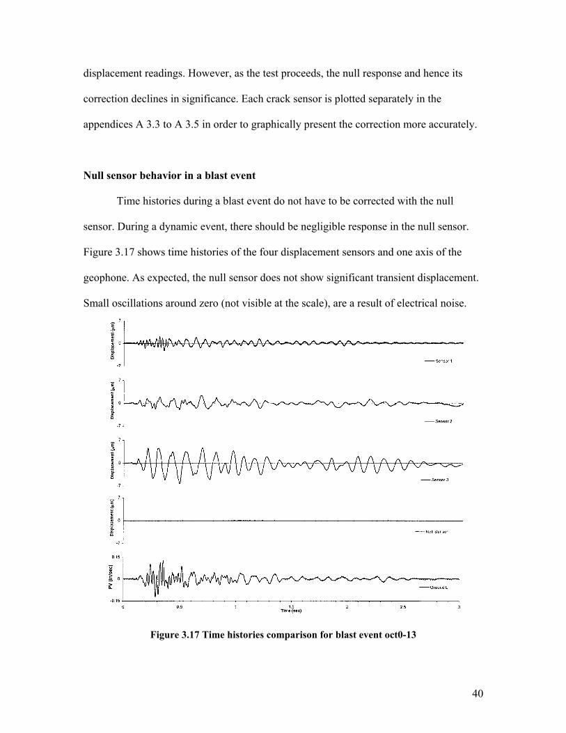
NORTHWESTERN UNIVERSITY

Autonomous Crack Comparometer Phase II

A Thesis

Submitted to the Graduate School In Partial Fulfillment of the Requirements

For the Degree

MASTER OF SCIENCE

Field of Civil Engineering

By

Michaël Louis

EVANSTON, IL

December 2000

ACKNOWLEDGEMENTS I would like to express my sincere gratitude to my advisor Professor Charles H.

Dowding, whose guidance and enthusiasm made this year at Northwestern University an

enriching and unforgettable experience.

Sincere thanks are also extended to Professor Richard J. Finno and Professor

Howard W. Reeves who reviewed my work and served on the committee.

I would like to gratefully acknowledge Mr. Daniel Aucouturier, Secrétaire

Général of the Fédération National des Travaux Publics (FNTP) for providing financial

support, Mr. Serge Eyrolles, chairman of the Ecole Spéciale des Travaux Publics (ESTP)

and Professor Raymond J. Krizek who organized the exchange program between the two

universities.

Thanks are also given to the staff of the Infrastructure Technology Institute and in

particular Dan Marron for all his advice and assistance during the project.

I would like to thank my friends Benoit, Laurelle, Stephane, and Jacques who

helped to make this year an enjoyable period of my life. Furthermore, I want to thank all

my fellow graduate students at Northwestern University for their support and friendship,

including Sebastian Bryson, Michele Calvello, Jejung Lee, Hsiao-chou Chao, Dan Priest,

Peter Babaian, Jill Roboski, Matthew Fortney, Bill Bergeson, Tanner Blackburn, James

ii

Lynch, and Helsin Wang. Good luck to Laureen McKenna who will take over this

research.

My parents, Anne-Marie Louis and Jean-Pierre Louis, my grand parents merit

special thanks for giving me their constant support and love. This exceptional experience

would not have been possible without their help.

Finally, I would like to dedicate this work to my brother Raphaël who would have

been so happy and proud to see me with this degree. I will never forget his joy and his

generosity. Raphaël, this work is for you in memory of your support and your constant

kind-hearted spirit.

iii

ABSTRACT

The thesis describes the second phase of development of the Autonomous Crack

Comparometer (ACC) system to incorporate measurements of ground motions and add

several changes in the autonomous operation. In order to obtain the ground motion and

air blast data, four additional transducers have been added. There are now a total of ten

channels of data autonomously collected and comparatively displayed by ACC. The web

page has been fully developed and now dynamic blast effects are compared with long-

term effects. Data are password protected. Finally, new data acquisition system software

has been installed that allows direct modem communication. The ACC installed in this

second test house allowed measurements, which verified past experience that daily and

weekly weather related crack displacements are greater than those produced by dynamic

events, whether they are household activities or blasts. Frontal (weekly) weather changes

produce the greatest crack response. Five different crack displacement sensors were

evaluated to determine the magnitude of thermal hysteresis and long-term electronic drift.

The eddy current sensor (9000 series) and the LVDT sensor were found to be acceptable

to measure micrometer displacements.

iv

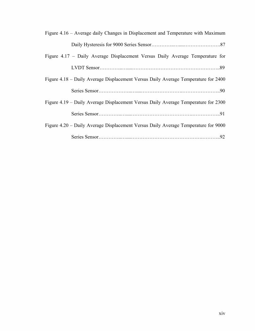
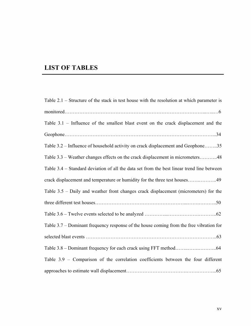
TABLE OF CONTENTS Acknowledgment………………………………………………………………………….ii

Abstract…………………………………………………………………………………...iv

Table of Contents………………………………………………………………………….v

List of Figures……………………………………………………………………………..x

List of Tables…………………………………………………………………………….xv

Chapter 1 – Introduction……………………….…………………………………….….1

New Approach to Vibration Monitoring…………..……………………..………1

Phase I Configuration………………...……………………………………...……2

System Development Led to Phase II Configuration………...…….…………….3

Focus of Thesis…………………………….………………..………….………....3

Chapter 2 – Phase II ACC as Installed in Test House Two………………….……..……..4

Introduction………………………………………………………..………………4

Hardware………...………………………………………………………………...5

Computer Instrumentation on Site..………………………….……………5

Data Acquisition System…………………………………………..5

Programming the DAS……………..……………………………...6

External Modem…………………………………………………..7

Micrometer Displacement Sensors…………………………...…………...8

v

Types of Sensors………………….…….…………………………8

Mounting Procedure………………………………………………9

Geophone: Ground Motion Sensor………………………………………..9

What Are the Characteristics of Ground Motion?……………...…9

Characteristics of the Sensor...………….………………………..10

Air Pressure Transducer………………………………………………….12

Characteristics……………………………………………………12

Conversion Factors………………………………………………12

Temperature and Humidity Sensor…………………….………………...13

Automated Data Collection Process………………………………………….….13

Control Polling Computer………………………………………………..13

Configuration…………………………………………………….13

Task Executed by the Polling Computer……..………………….14

Dynamic Generation of Graphs For The ACC Web Site……….……….15

Conversion Program Description………...……………………...15

Graphing Program……………………………………………….16

Web Site Changes……...……..………………………………………………….18

Opening Page………………………………………………….…………18

Site Specific Toolbar……………………………………………………..20

Future Work………………………………………………..…………….23

Null Sensor…...………………………………………………….23

Household Activities…………………………………………….23

Time Histories…………...………………………………………23

vi

Conclusion……………………………………………………………………….24

Chapter 3 – Measured Response of Test House Two………………………………….25

Introduction………………………………………………………………………25

Test House Description With Sensor Locations..…………………..……………26

Description………...………………………………………………….….26

Displacement Sensor Locations in the House……………………....……27

Outside Transducers……………………………………………………...31

Setting the Thresholds to Detect a Blast Event…………………………………..32

Blast Events……………………………………………………………...32

Electrical Noise of The Different Sensors…….…………….…………...34

Household Activity…………………………………..………………..…34

Thresholds…………………………………………....…………………..35

Crack Sensor Correction with Null Sensor………………………………..……..36

Correction for the Long-Term Data…………….……...………...………36

Null Sensor Behavior in a Blast Event…….……...……………….…….40

Crack Displacement Versus Weather…………………………...…………….…41

Correlation Between Crack Displacement and Temperature or

Humidity………………………………………………………..………..41

Separation of Daily and Weather Front Crack Response…………..……45

Sensitivity of Crack Displacement Versus Temperature and Humidity for

Different Test Houses……………………………………………………48

Standard Deviation of the Crack Displacement from The Best

Linear Trend Line…………………………………………….…48

vii

Daily and Weather Front Changes in Response……….………...51

Comparison of Environmental Effects and Blast Events on Crack

Displacement……………………………………………………………………..52

For Test House Two…………………………………………………..….52

For Book Test House and Test House Two…………………..…….……56

Comparison of Environmental Effects and Household Activity Effects on

Crack Displacement……………………………………………………...57

For Test House Two.....………………………………………….……….57

For the Three Different Test Houses…….……….……………………...60

House Structure Response……………………………………………………….62

Estimation of the Dominant Frequency Response of the House………...62

SDOF Analysis to Estimate Maximum Displacement of the Walls……..64

Comparison of Estimated Displacements and Ground Motion with Actual

Crack Displacements………………………...…………………………..65

Conclusion……………………………………………………………………….69

Chapter 4 – Comparison of Micrometer Displacement Sensors..……………………….70

Introduction………………………………………………………………………70

Micrometer Displacement Sensor Requirements and Crack Displacement

Definition…………...……………………………………………………………71

Micrometer Displacement Requirements……..………….……………...71

Crack Displacement Definition…………………..……………………...72

Test Description…...………………………………………...………………...…72

Comparison of Sensor Response with Theoretical Displacement.………72

viii

Mounting………………………………………………………….…...…73

Kaman Eddy Current Sensor (9000 Series)……………………………………...75

Fiberoptic Sensor from Philtec………………………….…………………….…75

Sensor Characteristics……………………………………………………75

Mounting…………………………………………………………………76

Test Results for The Fiberoptic Sensor…………………….…………………….77

Displacement Versus Temperature………………………………………………77

Cyclic Daily Hyteresis…………………………………………………………...83

Long-Term Electrical Drift………………………………………………………88

Conclusion………………………………………………………………….……94

Chapter 5 – Conclusions and Future Work……………………………………………....95

Summary…………………………………………………………………………95

Conclusions………………………………………………………………..…..…96

Future Work……………………………………………………………..…….....96

References……………………………………………………………………….….……98

Appendix 2: Mounting procedures for Kaman gages and Automate tasks to upload data

from the DAS and convert them into a text file……………………..A 2.1 – A 2.3

Appendix 3: Long term data, time histories, and transformed data………...A 3.1 – A 3.37

Appendix 4: Sensors data analysis…………………………………….……A 4.1 – A 4.1

ix

LIST OF FIGURES Figure 2.1 – Current ACC Configuration (Siebert, 2000)………………..……………….5

Figure 2.2 – Site Modem Scheme………………………...………………………….……7

Figure 2.3 – Dial Form Window to Call the DAS from the Polling Computer….....……..8

Figure 2.4 – Photograph taken in Test House Two showing That Eddy Current Sensors

Are Small and Do not Greatly Annoy the House Environment……….…….9

Figure 2.5 – Ground Motion Recorded in the Three Perpendicular Axis…………......…10

Figure 2.6 – Geophone View That Records Ground Motion……………………..…...…11

Figure 2.7 – Conversion between Volts and Particle Velocity……….………………….11

Figure 2.8 – Air Pressure Transducer Mounted in a Waterproof Box….………………..12

Figure 2.9 – Power Supply Board for Air Pressure Transducer……………….….……..12

Figure 2.10 – Chart Illustrating the Double Role of the Servlets Program……………....17

Figure 2.11 – Opening Page of the ACC Web Page……………………………………..18

Figure 2.12 – Crack Displacement Page that Defines Change in Crack Width…………19

Figure 2.13 – Household Activities Page that Compares Household Activity Effects with

Blasting Effects on the Crack Displacement………………………………20

Figure 2.14 – Site Page Showing the Specific Toolbar….………………………………21

Figure 2.15 – Page Proposing to the User, which Crack Sensor to See…………...….…22

x

Figure 2.16 – Comparison of Long-term and Ground Motion-induced Crack

Displacement…………………………………………………..…………...22

Figure 3.1 – Test House Two Front View……………...………………………………..26

Figure 3.2 – Plan View of the Test House…………………………………….………....28

Figure 3.3 – Elevation View of the Test House…………………………………….……28

Figure 3.4 – General Location of Crack Sensors 3 and 1…..…………………………....29

Figure 3.5 – Crack Sensor 3…………………………………….…………….………….29

Figure 3.6 – Crack Sensor 1………….………………………..…………………………29

Figure 3.7 – General Location of Crack Sensor 2 and Null Sensor ……...……………...30

Figure 3.8 – Crack Sensor 2……………………………………………………………...30

Figure 3.9 – Null Sensor………………………………………………………………....30

Figure 3.10 – Weather Transducers…...…………………………………….………...…31

Figure 3.11 – Geophone Location…………..…………………………………………...31

Figure 3.12 – Air Blast Transducer Location……………………………………………32

Figure 3.13 – Time Histories for the Smallest Blast Event………………...……..….….33

Figure 3.14 – Crack Sensors Versus Temperature from Sept 29th until Oct. 6th………...37

Figure 3.15 – Crack Sensors Versus Humidity from Sept 29th until Oct. 6th……………38

Figure 3.16 – Crack Sensors Correction Versus Time….………………...……..………39

Figure 3.17 – Time Histories Comparison for Blast Event Oct0-13…...………………..40

Figure 3.18 – Comparison of Crack Sensor 1 Displacement with Weather Changes…...42



xi

Figure 3.21 – Separation of Daily and Weather Front Crack Response for Crack 2 from

September 29 until October 06……………………………….……………46

Figure 3.22 – Separation of Daily and Weather Front Crack Response for Crack 2 from

September 16 until November 15…………………………….……………47

Figure 3.23 – Basement Crack Displacement Versus Temperature and Humidity for

Basement Sensor in the Sheridan Test House……………………………...51

Figure 3.24 – Comparison of Weather Effects and Blasting Effects on Crack 1………..53



Figure 3.27 – Comparison of the Maximum Blast-induced Displacement with Maximum

and Average Weather-induced Crack Displacement……...……………….56

Figure 3.28 – Comparison of Crack Time Histories for Typical Blast Event (0.09

inch/sec) and Slamming Main Entrance Door Event………….….……….58

Figure 3.29 – Comparison of Crack Time Histories for Typical Blast Event (0.09

inch/sec) and Running in the Living-Room Event………….….………….59

Figure 3.30 – Comparison of Environmental Effects and Household Activity Effects on

Crack Displacement…………………………….……………..…………...61

Figure 3.31 – Example of Free Vibration in the Crack Response……...……….……….63

Figure 3.32 – Comparison of Measured Displacement in the Crack with Estimated

Displacement of the Ground or the Wall for Crack 1…………….………..66

Figure 3.33 – Comparison of measured Displacement in the Crack with Estimated

Displacement of the Ground or the Wall for Crack 2……………….……..67

xii

Figure 3.34 – Comparison of measured Displacement in the Crack with Estimated

Displacement of the Ground or the Wall for Crack 3...…………..………..68

Figure 4.1 – Crack Displacement Definition (Siebert, 2000)….………...………………72

Figure 4.2 – Sensor Mounted on an Aluminum Plate between Two Aluminum

Brackets………………………………………………………………….....74

Figure 4.3 – Elevation, Top, Plan, and 3D Views of the Aluminum Bracket receiving the

Sensor- Dimensioning in Inches…...………………………………………74

Figure 4.4 – Eddy Current Sensor from Kaman (9000 Series)……………………..……75

Figure 4.5 – Fiberoptic Sensor from Philtec……………………..…………...………….76

Figure 4.6 – Screw Mounting………………………………..…………………………..76

Figure 4.7 – Ring Mounting………………………………..……………………………76

Figure 4.8 – Stiff Mounting………………………………..…………………………….76

Figure 4.9 – Displacement versus Temperature for the LVDT (6-day Test)..…………...79

Figure 4.10 – Displacement versus Temperature for the 2400 series (19-day Test)….....80



Figure 4.13 – Average Daily Changes in Displacement and Temperature with Maximum

Daily Hysteresis for LVDT Sensor……...…..…..…....……………………84


Daily Hysteresis for 2400 Series Sensor...………..………………………..85


Daily Hysteresis for 2300 Series Sensor…………..…...…………………..86

xiii

Figure 4.16 – Average daily Changes in Displacement and Temperature with Maximum

Daily Hysteresis for 9000 Series Sensor…………..…....………………….87

Figure 4.17 – Daily Average Displacement Versus Daily Average Temperature for

LVDT Sensor…………..…....……………………………………………..89

Figure 4.18 – Daily Average Displacement Versus Daily Average Temperature for 2400

Series Sensor………………..…....…………………….…………………..90


Series Sensor…………..…....……………………………….……………..91


Series Sensor…………..…....…………………………………….………..92

xiv

LIST OF TABLES Table 2.1 – Structure of the stack in test house with the resolution at which parameter is

monitored…………………………………………………………………………...…..…6

Table 3.1 – Influence of the smallest blast event on the crack displacement and the

Geophone………………………………………………………………………………...34

Table 3.2 – Influence of household activity on crack displacement and Geophone……..35

Table 3.3 – Weather changes effects on the crack displacement in micrometers………..48

Table 3.4 – Standard deviation of all the data set from the best linear trend line between

crack displacement and temperature or humidity for the three test houses…….………..49

Table 3.5 – Daily and weather front changes crack displacement (micrometers) for the

three different test houses………………………………………………...…….………..50

Table 3.6 – Twelve events selected to be analyzed …………...……………….………..62

Table 3.7 – Dominant frequency response of the house coming from the free vibration for

selected blast events ……………………………………………………………………..63

Table 3.8 – Dominant frequency for each crack using FFT method……..…….………..64

Table 3.9 – Comparison of the correlation coefficients between the four different

approaches to estimate wall displacement……………………………….…….………...65

xv

Table 4.1 – Comparison of the average of the daily hysteresis with the difference between

the maximum and the minimum daily average displacement…………….…….………..83

Table 4.2 – Comparison for each sensor of standard deviation of the average

displacement and temperature relationship from the best linear trend line…….………..88

xvi

CHAPTER 1

INTRODUCTION

NEW APPROACH TO VIBRATION MONITORING

Public fear of the possibility of vibration-induced cracking has led to a new

technology in vibration monitoring: an Autonomous Crack Comparometer (ACC). The

ACC technology focuses on monitoring the response of an existing crack because

observing crack response is easier than trying to determine the cause of cracking, which

is a very complex phenomena involving many parameters.

The main goal of the ACC system is the graphical comparison of crack

displacements produced by weather changes, blast-induced ground motion, household

activity, and other environmental effects such as thunder. As shown in case studies

(Dowding, 1996), the effects of temperature and humidity are much larger than

commonly thought by those with little background in structural investigation. Their

relative importance can be appreciated by comparing their effect on crack displacement

with that produced by blasting. The ACC is designed to be employed in houses or

buildings near quarries, mines, or construction sites. It is hoped that accessible graphs

1

will bring to involved parties information necessary to directly compare blasting effects

with those generated by weather.

The ACC project began several years ago. The phase I configuration system is

fully described by Siebert (2000). Developments and improvements involved in the phase

II configuration are the focus of this thesis.

PHASE I CONFIGURATION

Phase I was the first step of developing equipment and software necessary for the

system. The basic equipment consists of a hardware including a data acquisition system,

an on-site computer, micrometer proximity sensors, and weather sensors.

Data transfer from the field site to a server via computer modem is automated.

The AutoMate (Unisyn, version 4.5, 1999) program enables collection of long-term and

household vibration data every day and subsequent storage as text files. All computations

are made at the server in order to avoid taxing field units in anticipation of eventually

combining operations with existing commercial equipment.

Java programs display long-term crack displacement on the Internet on a web

page designed for easy access by the average computer. Use of serverside applets ensure

the accessibility of data by any browser and so assures the widest audience. The web

page presents an attractive image of simple and quickly transmitted graphics that are easy

to understand. This simplicity allows access by the oldest of computers still in operation.

Sidebars do not consume horizontal space and they can remain on all screens so viewers

do not need to recall possible options. Background information is provided to inform

public about the theory behind this technology. Graphs are updated every day.

2

SYSTEM DEVELOPMENT LED TO PHASE II CONFIGURATION

The phase II system configuration is based on ACC phase I technology but, in this

phase the system was updated and moved to a house adjacent to an operating quarry. The

Test House Two will refer here and after to the quarry Test House. Additional

development includes the following: 1) Addition of geophones to record ground motions

and an air pressure transducer to record blast-air over pressure. 2) Direct modem

communication between the site and the server through new data acquisition system

software. 3) Several changes in the autonomous operation. 4) Graphical comparison of

dynamic effects with long-term effects on the crack displacement. 5) Addition of a

password protection to ensure control of the data.

FOCUS OF THE THESIS

Chapter two describes in detail the phase II Autonomous Crack Comparometer as

installed in the second test house. It focuses on the development and improvements upon

the phase I system. Chapter three deals with the measured response at the new test house

(two). These results are compared to past case studies and similar test houses. Chapter

four compares attributes of the sensors considered to measure micrometer displacements,

and evaluates their reliability with respect to long-term behavior. Finally, Chapter five

summarizes the accomplishments and the limitations of the current system in order to

recommend future improvements of the ACC. Complete records of data as well as

program details are contained in a separately bound appendix.

3

CHAPTER 2

PHASE II ACC AS INSTALLED IN TEST HOUSE TWO

INTRODUCTION

The current Autonomous Crack Comparometer (ACC) as installed in Test House

Two is based on the technology developed in Sheridan Road Test House, which is fully

described by Siebert (2000). Figure 2.1 illustrates the ACC concept. Vibrations produced

by ground motion, and household activities as well as weather changes are automatically

monitored and compared with changes in crack width. Via the Internet, graphs are

available on a web site. This chapter focuses on system development necessary for data

transfer, and web site improvements. The main addition is monitoring of ground motion

and the air pressure variation in order to compare long-term crack induced displacement

with that induced by ground motion and household activity. The presentation describes in

detail only those changes made to the system described in Siebert (2000).

4

Self-triggered Vibration Monitor

Micrometer Crack Gage(s) Long-term and Vibration Displacement

Neighbors/Owners/ Regulators

Server Autonomously Produces WWW Graphical

Comparison

Figure 2.1 Current ACC configuration (Siebert, 2000)

HARDWARE

Instrumentation on site

Data Acquisition system

The Data Acquisition System (DAS) for Test House Two is based on the same

SOMAT platform as described in by Siebert (2000). However, the processor “Turbo

2100” is new. It can now be attached directly to an external phone modem. Thus, via a

phone modem, the DAS can be polled from any modem-equipped phone computer with

software WINTCS 2 provided by SOMAT. Therefore, an additional computer on site is

no longer needed, as was the case for the system described by Siebert (2000). The DAS is

made of layers of sensor inputs, which are stacked together described in Table 2.1.

5

Layers Filters Filter type TT

Type Resolution

Displacement crack 1 - 12 bit 0.1 µm Displacement crack 2 - 12 bit 0.1 µm Displacement crack 3 - 12 bit 0.1 µm Null sensor displacement - 12 bit 0.1 µm Temperature Yes 8 bit 0.4 °Celsius Humidity Yes 8 bit 0.4 % Geophone L axis - TT 8 bit 0.002 in/sec (0-p) Geophone T axis - TT 8 bit 0.002 in/sec (0-p) Geophone V axis - TT 8 bit 0.002 in/sec (0-p) Air blast transducer - 8 bit 0.0004 psi (0-p) 4 Megabytes memory Turbo processor

TT: four-point average to trigger

Table 2.1 Structure of the stack in test house with the resolution at which the parameter is monitored

The master sample rate of the DAS for each sensor is 1000 samples per second, or

a reading is taken every millisecond. Two types of multiple point time histories are

produced. The first one is employed to compare crack displacement with weather

changes (See Chapter 3) and records samples for each channel every hour. The second is

used to produce time histories of crack displacement, ground motion, and air pressure

when a dynamic event occurs. Triggers that start this type of data collection are set to

trigger only on ground motion as described in Chapter 3. These time histories are

recorded for three seconds yielding 3000 data points.

Programming the DAS

In order not to record events that are not blast induced, the DAS is programmed to

trigger on the average of the four last data points. This average is then compared to the

threshold values for triggering. If it is greater than the threshold, the DAS triggers and

6

records a three-second signal for all channels except the temperature and the humidity. If

the average is lower than the threshold, the DAS does not trigger. To ensure that the

entire signal is recorded, the three seconds of record begin 0.1 second before the trigger

(Siebert, 2000).

External modem

In order to access the DAS from any computer, a modem (shown in Figure 2.2)

that transfers data at a maximum rate of 33.6 kilobits per second, is necessary on site.

Figure 2.2 Site modem scheme

The modem is connected to the DAS with a null modem adapter and to a phone line. The

procedure to call the DAS is to open WINTCS in the Polling Computer (discussed further

in this chapter), select “modem” in the toolbar and click on “hang on”. Then a window

(shown in Figure 2.3) called “dial form” appears.

7

Figure 2.3 Dial form window to call the DAS from the Polling Computer

The phone number is written in the first box. The modem configuration is specified in the

second box. When “dial” is clicked, the communication is established. Modems can

transfer data only if they are compatible and if they use the same language. Moreover,

they need to interface at the same baud rate. The external modem has been programmed

on site with a laptop via a serial cable to meet these requirements.

Micrometer displacement sensors

Types of sensors

Four 9000 series eddy current sensors from Kaman are employed in Test House

Two. They showed acceptable thermal hysterisis and electrical drift of the three eddy

current sensors tested, as shown in Chapter 4. In addition, they are small and easy to

install, which minimizes disturbance to the home owner. The small size of the sensor and

electronics can be seen in Figure 2.4. A 15 VDC power supply feeds the four sensors.

8

s

Figure 2.4 Photograph taken in Tesmall and do not g

Mounting procedure

Mounting brackets are descr

mounting and calibration procedure,

Geophone: ground motion sensor

What are the characteristics of grou

The ground motion sensors (

ground along three perpendicular ax

(V). The amplitude of a blast-induce

Velocity (PPV) and the frequency at

electronic
sensor
st House Two showing that eddy current sensors are reatly annoy the house environment

ibed in Chapter 4. Kaman gages used a specified

which is available in appendix A 2.1.

nd motion?

geophones) record the velocity of particles in the

is; Longitudinal (L), Transversal (T) and Vertical

d ground motion is characterized by the Peak Particle

which it occurs. PPV is the maximum particle

9

velocity measured “zero to peak”. Figure 2.5 shows an example of ground motion

recorded in test house 2. The horizontal axis represents the time from 0 to 3 seconds.

Peak Particle Velocity

Figure 2.5 Ground motion recorded in the three perpendicular axis

For the example in Figure 2.5, the PPV in the T direction is equal to 0.13 inch per second,

and the frequency at which it occurs is around 31 Hertz.

Characteristics of the sensor

Geosonics Inc. manufactures this geophone shown in Figure 2.6 from three third

party transducers. While this device does not need any power supply, it generates a high

level of electrical noises, because of the unusually long (12 meters, 40 feet) connection

cable between the DAS and the geophones mounted outside below the ground level.

Typical electrical noise amplitudes are 0.005 inch per second and are filtered out with the

four-point average trigger condition as discussed previously in this chapter.

10

Figure 2.6 Geophone view that records ground motion (Geosonics Inc.)

The conversion between volts (output signal) and particle velocity in inch per second

must also include a conversion between “peak to peak” output voltage and “zero to peak”

PPV. Figure 2.7 illustrates this conversion.

-1.5

0

1.5

0 2 4 6 8 10

Time (seconds)

Parti

cle

velo

city

(in/

sec

0 to

pea

k)

-1.2

0.0

1.2Vo

lts (p

eak

to p

eak)

1 in/sec Zero to peak

1.550 volts peak to peak

Figure 2.7 Conversion between volts and particle velocity

.

11

Air pressure transducer

Characteristics

The differential air pressure sensor used in Test House Two is manufactured by

Sensym. It measures the variation in audible and inaudible atmosphere pressure

associated with the blast noise. This device requires an 8 VDC +/- 0.01 volts power

supply, which is somewhat unusual. The power supply had to be designed and built by

ITI personnel because they were not available on the market. Figure 2.8 shows the

transducer mounted in a waterproof box. The difference in air pressure is evaluated

between the two sensors protruding out of the cap. Figure 2.9 shows the board built to

supply the transducer with 8 VDC.

Figure 2.8 Air pressure transducer mounted in a waterproof box

Figure 2.9 Power supply board for air pressure transducer

Conversion factors

The air pressure response is given in volts by the transducer, which is easily

converted to pounds per squared inch. One millivolt corresponds to 0.0001 psi “zero to

12

peak”. Pressure must then be transformed into decibels with the following formula

(Dowding, 1996):

( )

= − psix

psiPdB 910 109.2log20 ,

where P in pounds per squared inch (psi) refers to the peak measured sound pressure

“zero to peak”.

Temperature and humidity sensor

Characteristics and mounting procedures are fully described by Siebert (2000).

AUTOMATED DATA COLLECTION PROCESS

Since the basic process is fully described in Siebert (2000), the discussion will

focus on the changes required to integrate ground motion and air-blast excitation.

Automate (Unisyn, version 4.5, 1999) continues to be employed to execute tasks

automatically. PCAnywhere (Symantec, version 9.2.1, 2000) is no longer necessary as

version 2, the Somat DAS software, now supports modem communication.

Control Polling Computer

Configuration

The configuration of the Polling Computer has been modified for this project. The

software WINTCS 2 (SoMat, version 2.0.1, 2000) was set up under the Windows 98

operating system for greater stability and efficiency. The Polling Computer is equipped

with a 56k modem in order to communicate with the DAS. The hard drive is about 10

Gigabytes and must save 2 Megabytes of files each day. Moreover, the Polling Computer

13

also is attached to the ITI network in order to share the data and text files with the server

computer that displays the graphs on the ACC web page.

Tasks executed by the Polling Computer

Details of polling tasks can be found in appendix A 2.2. The Automate task

program runs every day at 10:30 PM. Steps 1 to 25 transfer data from the DAS to the

Polling Computer. Steps 26 to 45 convert the data file into a text file.

Steps 1 to 6 start WINTCS 2 program and open the “command entry” window,

which is the critical step because of software issues. Therefore, steps 7 to 11 enable the

“command entry” window by pressing the “F4” key, in case this window did not appear

with steps 1 to 6. However, even this approach is not completely reliable. This reliability

deficit will be improved with the professional version of Automate, which allows

conditional tasks. Once the “command entry” is active, Automate goes through the steps

12 to 25: Basically, first the DAS is automatically dialed by the Polling Computer to

establish a communication between the site and the laboratory. Second, the DAS stops

the test, uploads the data to a shared directory on the Polling Computer, and initiates a

new test.

Steps 26 to 35 delete any data file already loaded in the EASE program. This is a

precaution. Steps 36 to 41 load the data file available on the shared directory and save it

as a text file on another shared directory accessible by Java programs described in the

following paragraph. Steps 42 to 45 clear the different channels and close the EASE

program (SoMat, version 3.03.10, 2000).

14

Dynamic generation of graphs for the ACC web site

Text files saved on the Polling Computer are used to automatically produce the

comparative graphs that are displayed on the ACC web site. Several improvements have

been made in this second phase. The conversion program has been made more flexible.

The rate at which graphs are displayed has been increased. Labels on time axis have been

improved, and password protection for individual sites has been added.

Conversion programs description

Java programs have been written (Kosnik, 2000) for displaying and comparing

both long-term (weather related) and dynamic (blast and household activity) data. Basic

to both types of data is the conversion of time and date to Julian time for computer

storage. Also basic to both types of data is the conversion of crack displacement sensor

voltage to micrometers. Since the same sensor measures both, the conversions are the

same. Temperature and humidity conversions are unnecessary.

Long-term data are differentiated from dynamic data by their order in the text file.

A single long-term data point for each crack sensor and time of reading is stored along

with the Julian time of recording. Both a 3000-point time history and a maximum

absolute value “zero to peak” value are produced for the dynamic crack response. A

similar program is employed for the ground motion and air blast data.

The cause of dynamic events needs to be determined. As explained in Chapter 3,

vibration events can be triggered by blast events, electrical noise events, and household

activity events. Most importantly electrical noise events need to be eliminated. First the

15

four-average data point trigger eliminates most of the spike noise events. A further

precaution is undertaken. Data are stored in a temporary data table. For each event,

maximum and minimum are evaluated then added. Blast or household activity events are

relatively symmetrical around zero. For an event to be electrical noise, the sum of the

maximum and the minimum must be greater than 0.03 inch per second. So far, this error

check condition has been reliable at 100 percent. This involved two months of testing

from September 16 until November 15 and thirty-one blast events. It is envisioned that

similar logic will be developed to autonomously distinguish household activity, thunder,

etc.

Graphing program

Graphs are produced by Java programs called “servlets”. The flowchart for these

in Figure 2.10 illustrates the double role of the servlets. They have two functions; A and

B. Function A is to plot graphs from blast events available in the database and to return a

GIF image. Function B is to control the flow of data between the user’s web browser and

the database.

16

User’s web browser

ITI server @ iti.birl.nwu.edu

Plot data from database to return a

GIF image

User sees either the graph or login required sign

Return a GIF image Transfer the graph request from user via the internet

Request a graph

A

Check password- If logged in, get blast dadatabase - If not logged in, return lofile from database

User

Figure 2.10 Chart illustrating the double role of the servlets prog

Servlets
Server submit request to
the servlets
B
: ta from

gin return

ram

17

WEB SITE CHANGES

Opening page

The structure of the opening page, seen in Figure 2.11, is the same as in phase I

with the consistent banner and the left side choice bar. However, new links can be visited

under the “Purpose of Project” directory. Moreover, another monitoring site is available.

The Northwestern University logo has been removed to speed downloading on older

machines.

Figure 2.11 Opening page of the ACC web site

One of the links available under “Purpose of Project” is “Crack displacement”.

This link refers to the definition of the crack displacement illustrated by a scheme. It was

important to understand that the crack width change (not crack width) is measured as

shown in Figure 2.12.

18

Figure 2.12 Crack displacement page that defines change in crack width

Another new link is “Human Effects” or “Habitation Vibrations”. The table seen

on Figure 2.13 compares the habitation vibrations with a blast event. This table

demonstrates that blasts often affect the crack displacement less than everyday actions

inside the house.

19

Figure 2.13 Household Activities page that compare household activity effects with blasting effects on the crack displacement

Site specific toolbar

As soon as a site is chosen in the opening page, a page appears with a left-hand

bar, shown in Figure 2.14, that is the same for each site page. A login and a password are

required in order to display information for sites other than test house on the

Northwestern campus. If the user does not log in, he will not see the graphs that compare

crack displacement with weather changes, household activities, and blast events.

However, the “Purpose of Project” section is still visible.

One of the new links is “Household Activities” in the “Crack Displacement

Induced by:” directory. This option will compare the crack displacement generated by

everyday life inside a house to daily or seasonal displacements due to weather changes.

This option will be developed during the next phase

20

Figure 2.14 Site page showing the specific toolbar

Another link is “Ground Motion” in the “Crack Displacement Induced by:”

directory. Figure 2.15 shows that when the link is clicked, a new page appears and

requests the user to choose the crack sensor of interest. Figure 2.16 is the page that

appears when the user picks a specific crack sensor. This graph includes a caption to

explain the method of comparison. This plot compares long-term crack displacement

(blue), with displacement induced by ground motion (green). Dark blue and light green

colored points were chosen to represent the effects of ground motion to avoid

21

Figure 2.15 Page proposing to the user, which crack sensor graphs to see

Figure 2.16 Comparison long-term and ground motion induced crack displacement

22

alarming reds or yellows. Dark (and light) green points represent the maximum positive

(and negative) excursions from the long-term crack position produced by the vibration

event. As discussed in Chapter 3, these dynamic changes are small compared to those

produced daily and weekly weather changes.

Future work

Null sensor

Long-term crack displacement will be corrected by subtracting null sensor

displacement as shown in Figure 3.16. In addition, null sensor time histories will be

included with crack and ground motion time histories. These time histories can be chosen

from a data table that will be presented when “Time History” (at the bottom of the left

hand choice bar) is chosen.

Household activities

Graphs shown in Figure 2.16 will be necessary to compare long-term induced

crack displacement with household activity-induced displacement. Each vibration event

will have to be isolated and identified as a blast or a household event. In addition

provisions will have to be made to allow the entire system to be triggered if an individual

crack sensor threshold level is exceeded.

Time histories

For this graph (as yet undeveloped) the first step would be to give examples of

time histories coming from different types of events. All responses: crack displacement,

23

ground motion from each axis, and air pressure variation would be compared on a

common time base. The ultimate goal is to provide the viewer the time histories for each

event by clicking on one of green dots plotted in the “Crack Displacement Induced by”

graphs. Interested parties could analyze the impact of those events and jump from one

event to another to make quick comparisons.

CONCLUSION

The second phase of development of the Autonomous Crack Comparometer

(ACC) system incorporated measurements of ground motions and several changes in the

autonomous operation. In order to obtain the ground motion and air blast data, four

additional transducers have been added. There are now a total of ten channels of data

autonomously collected and comparatively displayed by ACC. The left hand device bar

on the web page was expanded and modified for clarity. The “Purpose of the Project”

choice has been expanded and changed. Dynamic effects are compared with long-term

effects under the choice “Crack Displacement Induced by”. Comparisons from “Ground

Motion” have been fully developed. Password protection has been added to ensure

quality of the data. Finally new data acquisition system software has been installed that

allows direct modem communication.

24

CHAPTER 3

MEASURED RESPONSE OF TEST HOUSE TWO

INTRODUCTION

Chapter 3 describes response of Test House Two, which is located adjacent to an

aggregate quarry. As opposed to the Sheridan house, ground motion and air pressure

variations are recorded. The purpose of this chapter is to compare crack movements

produced by blast-induced ground motion with those produced by environmental effects

or by household activities. These results will be compared to those obtained at other test

houses. In addition the crack response of the structure will be analyzed to find dominant

frequencies of the house. Finally, the crack responses are compared to various descriptors

of ground motion in order to find correlations.

Summarizing tables and condensed graphs are presented in this Chapter.

Vibration event samples and graphs coming from data transformed are shown in the

appendices.

All the electronic data are stored in the polling computer. A backup on a CD is

made. To analyze the house response, time histories, Fast Fourier Transforms, Single

25

Degree of Freedom analysis have been produced from electronic data and they have been

recorded on a CD.

TEST HOUSE DESCRIPTION WITH SENSORS LOCATIONS

Description

The backyard of Test House 2 (shown in Figure 3.1) is adjacent to on an

aggregate quarry. The quarry boundary is at the end of the back yard and blasting

operations are around 600 meters (2000 feet) far from the test house. It is a one-story,

concrete masonry block structure with a concrete masonry block basement that opens out

to a backyard one story below the front yard. Figure 3.11 shows the slope between front

and back yard. A garage is located next to the house, but there is no connection between

the two structures. As shown, the exterior walls are faced with stone.

Figure 3.1 Test House Two front view

26

The first floor joists are supported by a wooden principal beam running

lengthwise. The ceiling is supported by transverse wooden joists which are supported at

the center by a wall that sits on top at the support beam.

Displacement sensor locations in the house

Three eddy current crack sensors span three different cracks and a null sensor is

mounted on an uncracked wall section as shown in Figure 3.2 and 3.3, plan and elevation

views respectively. The general locations of crack sensors 1 and 3 are shown in Figures

3.2, 3.3 and 3.4. Sensor 1, details of which are shown on Figure 3.5, is located in the

living room at the top of the wall separating the kitchen and the living room. It spans a

crack that seems to be created by expansion and contraction of the beam supporting

ceiling joists above the wide opening between the living room and the kitchen. Sensor 3,

details of which are shown on Figure 3.6, is located at the top of the wall separating the

main entrance hall and the living room. As with sensor 3, this sensor spans a crack that

seems to be caused by expansion or contraction of the beam spanning the opening from

the entrance to the living room.

The general locations of the crack sensor 2 and the null sensor are shown in

Figure 3.7. Sensor 2, details of which are shown in Figure 3.8, is mounted on a long

ceiling crack in the computer room. The null sensor, details of which are shown in Figure

3.9, is located above the door separating the main entrance hall and the computer room

on an uncracked wall section. It was mounted in that location to be as close as possible of

the other sensors and at approximately at the same height on the wall.

27

Computer room

Kitchen

Living room

Sensor 1

Sensor 2

Null SensorSensor 3

Main entrance door

Cabinet

BASEMENT

ROOFNull Sensor

Sensor 2Sensor 3

Sensor 1

Bedroom 1

Bedroom 2

Bathroom

Wooden deck

Geophone

Air pressure transducer

Figure 3.2 Plan view of the test house

Figure 3.3 Elevation view of the test house

28

Figure 3.4 General geometry of crack sensors 3 and 1

Figure 3.5 Crack sensor 3


Electronics

29

Figure 3.7 General geometry of crack sensor 2 and Null sensor


Figure 3.9 Null sensor

Electronics

30

Outside transducers

The weather transducer, shown in Figure 3.10, measures temperature and

humidity. It is mounted on the junction box, which contains the circuitry that provides

power and transmits output to the Data Acquisition System (DAS). While its location just

below the wooden deck protects it from intense rains, it may have lead to artificially high

humidity readings.

The 3-axis geophone that measures the ground motion was buried six inches

below the ground. The shovel seen on Figure 3-11 shows the exact location of the

Geophone. It is quite close to the wooden deck and therefore can sense outside household

activities.

The air blast transducer was mounted at the end of the deck. Figure 3.12 shows

the location of this sensor.

Junction box

Weather transducer

Geophone

Figure 3.10 Weather transducers

Figure 3.11 Geophone location

31

Air blast transducer

Figure 3.12 Air blast transducer location

SETTING THE THRESHOLDS TO DETECT A BLAST EVENT

Blast events

A blast event produces ground vibrations and crack movements. The ground

motion and response is recorded as time histories as shown in Figure 3.13. All discussion

herein is based upon the “zero to peak” value, which is the absolute distance of the

maximum excursion from zero. Time histories from one of the lowest intensity ground

motions are shown in Figure 3.13. These are three-second time histories.

32

Figure 3.13 Time histories for the smallest blast event

Table 3.1 summarizes the maximum “zero to peak” value for the crack sensors and for

each axis of the geophone for Figure 3.13. Therefore, to detect a blast event larger than

this smallest event, the thresholds should be set above 1-micrometer movement for the

sensors and 0.02 inch per second velocity for the geophone. L, T, and V respectively

stand for Longitudinal, Transversal, and Vertical.

33

Crack sensors Geophone #1 #2 #3 L T V

“zero to peak” displacement (micrometers)

0.5 0.4 1.0 - - -

PPV (inch/second) - - - 0.02 0.03 0.02

Table 3.1 Influence of the smallest blast event on the crack displacement and the Geophone

Electrical noise of the different sensors

Background electrical noise, associated with any electrical system affects the

output signal and the resolution. Regular noise usually has a constant frequency and

oscillates around zero. Thus a simple filter could eliminate it. However, in Test House

Two, the outside sensors, especially the geophone, showed recurrent irregular electrical

noise with large spikes in the signal. Some examples of noisy signals from the Geophone

and the crack sensors are shown in the appendix A 3.1. Also in appendix A 3.2 is the

typical level of electrical noise for each sensor and the maximum spikes amplitude that

can reach 0.25 in per second. These false events were filtered by triggering on a four-

sample average as explained in Chapter 2. Although this filter was very efficient, some of

the false events were of such magnitude that they were not filtered out.

Household activity

Everyday life in a house perturbs wall cracks. Outside activities in the backyard

around the geophone can also generate vibrations in the ground. If the thresholds for the

sensors are not set specifically for a blast event, the DAS will be triggered and record

these vibrations. To address this, several household activity vibrations have been

34

simulated. Table 3.2 represents the value “zero to peak” recorded for each of six example

household activities. They can be compared to those for the smallest blast event shown in

Table 3.1. Household activities generate more displacement in cracks and more ground

motion than the smallest blast event. To preclude activity from triggering the DAS, the

crack sensors have been set to a passive condition. Only output of the geophone is

allowed to trigger the DAS.

CRACK SENSORS (micrometers) #1 #2 #3

Running in the living room 3.0 0.4 3.5 Slamming main entrance door 1.4 2.4 3.4 Slamming closet door 0.9 1.4 2.8 Smallest blast event 0.5 0.4 1.0

GEOPHONE (inch/second) L T V

Jumping above the Geophone 0.08 0.12 0.10 Running around Geophone 0.07 0.06 0.05 Running on wooden deck 0.04 0.05 0.06 Smallest blast event 0.02 0.03 0.02

Table 3.2 Influence of household activity on crack displacement and geophone

Thresholds

The system only triggers upon geophone thresholds. The threshold velocity has

been set at 0.02 inch per second for each of the three directions. However, data must still

be evaluated in order to eliminate electrical noise events as well as household activity

events.

The next phase of research will focus on autonomous distinction of household

activity and blast events. Both geophone and crack sensors can be employed to

distinguish blast response. Considering the system triggerable from both, crack response

35

only would indicate inside household activity. Ground motion only would indicate

outside household activity. Finally both ground motion and crack response would be a

blast-induced condition. Air blast only would be a result of thunder.

CRACK SENSOR CORRECTION WITH NULL SENSOR

Correction for the long term data

“Crack displacement” is defined by Siebert (2000) and in Chapter 4 (Figure 4.1).

The crack displacement refers to the changes in crack width rather than the entire crack

width.

Dowding (1996) and Siebert (2000) show that crack displacement data may need

to be corrected to compensate for thermal hysterisis and an electrical drift. Thermal

hysteresis is produced by material expansion that includes brackets, plaster and epoxy

volume variations.

To correct the crack sensor displacement for these effects, the null displacement

has to be subtracted. Figure 3.14 shows sensor response as a function of temperature.

When the temperature increases, the crack sensor displacement tends to decrease while

the null sensor displacement rises slightly. When compared to the humidity in Figure

3.15, the crack sensors and the null sensor behave similarly as in Figure 3.14. As

described earlier, the humidity value may be high as a result of placement under the

porch in a position that is unusually humid.

Figure 3.16 represents the displacement response of each crack sensor when the

null response is subtracted. The correction appears to be of any significance at all only at

the beginning of the data collection. The correction decreases the crack sensor

36

displacement readings. However, as the test proceeds, the null response and hence its

correction declines in significance. Each crack sensor is plotted separately in the

appendices A 3.3 to A 3.5 in order to graphically present the correction more accurately.

Null sensor behavior in a blast event

Time histories during a blast event do not have to be corrected with the null

sensor. During a dynamic event, there should be negligible response in the null sensor.

Figure 3.17 shows time histories of the four displacement sensors and one axis of the

geophone. As expected, the null sensor does not show significant transient displacement.

Small oscillations around zero (not visible at the scale), are a result of electrical noise.

Figure 3.17 Time histories comparison for blast event oct0-13

40

CRACK DISPLACEMENT VERSUS WEATHER

As mentioned and shown by Dowding (1996), crack displacement is correlated to

environmental changes in humidity and temperature. Siebert (2000) also confirmed this

observation with satisfactory correlation.

Correlation between crack displacement and temperature or humidity

In Test House Two, the temperature and the humidity were monitored outside the

house whereas the sensors were mounted on inside walls the house. Figures 3.18, 3.19

3.20 compare crack sensor displacements and weather changes. Crack 2 is the most

responsive to the environmental changes as it shows the largest displacement changes

compared to the two other cracks. Figure 3.20 shows that Crack 3 closed gradually in

October whereas it tends to be affected only by the daily changes in the first two weeks

of November. However, Cracks 1 and 2 average displacement reflecting weather fronts

show no such trend with time, even though they show daily changes caused by weather

effects. At the beginning of the heating season, Crack 3 has begun to show cyclic

behavior that may reflect response to house heating.

The humidity sensor constantly yields high values. Some of which are above 100

percent. As discussed before, this gage may have been improperly placed in a location at

relatively high humidity. Therefore, any comparison with humidity data must be made

cautiously.

Crack displacement and weather changes do not correlate well. The average long-

term temperature is dropping because of the change from summer to fall. The heating

system is probably turned on in the house, which provides a relatively constant inside

41

temperature, and decreases crack displacement correlation with outside temperature

because of the desiccation of the wood. The phase III ACC will include inside

temperature and humidity sensors.

Separation of daily and weather front crack response

Daily and weather front changes can be separated. An eight-day period, extracted

from Figure 3.19 is considered. This period starts on September 29 and ends on October

06. As shown on Figure 3.21, subtracting the eight-day trend (the eight-day long sine

wave obtained with a degree six polynomial trend line of the long-term crack response)

from the crack response yields the daily response. The eight-day trend is the effect of a

passing weather front.

As illustrated in Figure 3.22 for Crack 2, separation has been generalized over the

studied period (from September 16 until November 15) for the three cracks in Test House

Two. The method used was slightly different. Instead of employing a polynomial trend

line to fit the crack displacement as in Figure 3.21, the weather front changes or delayed

crack response have been calculated as follows: First, the crack displacement is averaged

for each day and each average data point is plotted versus time. Second these average

data points are connected and the line obtained is labeled “average displacement

reflecting weather fronts” as shown on Figures 3.18 to 3.20. Third, an average horizontal

line of this graph is drawn by eye. Fourth, the distance between this line and each peak of

the “average displacement reflecting weather front” line is recorded. The average of these

distances is given in Table3.3 as “Weather front changes”. The daily change graph is

obtained by subtracting the measured crack displacement from the graph labeled

45

“average displacement reflecting weather front”. Table 3.3, details of which are shown in

appendices A 3.6 to A 3.8, summarizes results of this procedure for the three cracks in

Test House Two. The table also compares daily and weather front crack displacement

with the maximum blast induced displacement. The maximum PPV in Table 3.3 was

associated with the event that produced the maximum displacement for the crack.

Crack 1 Crack 2 Crack 3 Average 7 24 12 Daily changes

Std deviation 4 14 8 Average 14 50 20 Weather front

changes Std deviation 7 16 14 Maximum household activity 3 2.5 3.5 Maximum blast-induced crack

displacement 4 7 9

Maximum associated PPV (in/sec)

0.09 0.08 0.09

Table 3.3 Weather changes effects on the crack displacement in micrometers

Sensitivity of crack displacement versus temperature and humidity for different test

houses

Cracks in two other houses are analyzed for weather effects. First, the Book Test

House is a case study from Dowding (1996). The second is the Sheridan Road Test

House from Siebert (2000). Plan and elevation views showing sensor location and house

descriptions are available in appendices A 3.9 to A 3.12.

Standard deviation of crack displacement from the best linear trend line

Simply plotting crack displacement versus temperature and humidity, a standard

deviation set from the best linear trend line of the entire data can be calculated. Figure

48

3.23 shows such a plot for the basement crack in the Sheridan House. Table 3.4 compares

these standard deviations of similar plots for five cracks in the three test houses. The

entire set of graph is presented in appendices A 3.13 to A 3.16.

Temperature Humidity Test House Crack

SE or σ* R2** SE or σ* R2** Book C7 13.39 0.3312 16.28 0.0275

Sheridan Basement 3.56 0.0291 2.33 0.5844 1 8.79 0.0234 8.77 0.0277 2 22.23 0.0206 22.46 0.0001 Two 3 14.75 0.0134 14.80 0.0067

* Standard Error in micrometers ** Correlation coefficient of the best fit linear trend line (dimensionless)

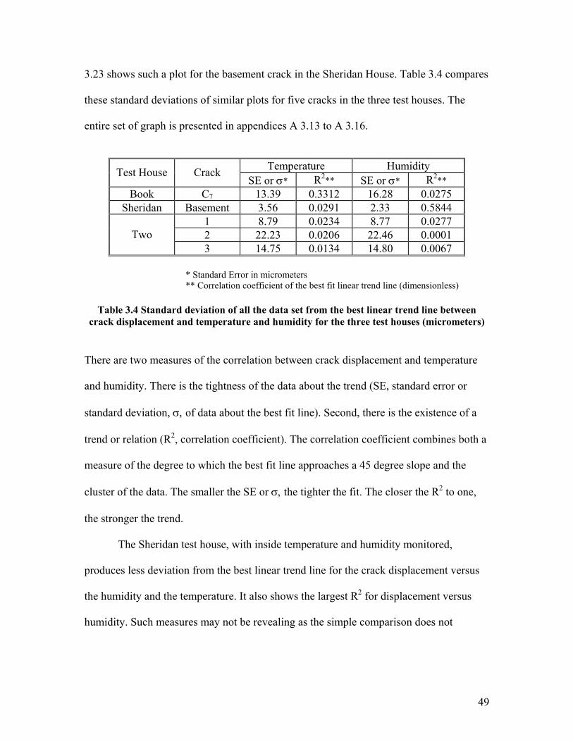
Table 3.4 Standard deviation of all the data set from the best linear trend line between

crack displacement and temperature and humidity for the three test houses (micrometers)

There are two measures of the correlation between crack displacement and temperature

and humidity. There is the tightness of the data about the trend (SE, standard error or

standard deviation, σ, of data about the best fit line). Second, there is the existence of a

trend or relation (R2, correlation coefficient). The correlation coefficient combines both a

measure of the degree to which the best fit line approaches a 45 degree slope and the

cluster of the data. The smaller the SE or σ, the tighter the fit. The closer the R2 to one,

the stronger the trend.

The Sheridan test house, with inside temperature and humidity monitored,

produces less deviation from the best linear trend line for the crack displacement versus

the humidity and the temperature. It also shows the largest R2 for displacement versus

humidity. Such measures may not be revealing as the simple comparison does not

49

account for time effects. As shown in Dowding (1996), crack response is a function of

intensity of humidity change and the length of time that change is in effect.

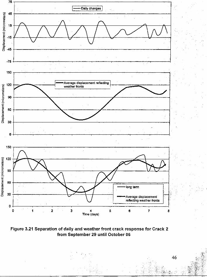
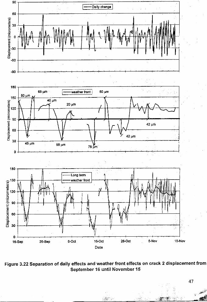
Daily and weather front changes in response

The generalized separation procedure between the daily changes and the weather

front changes in crack response explained before is also employed for the three different

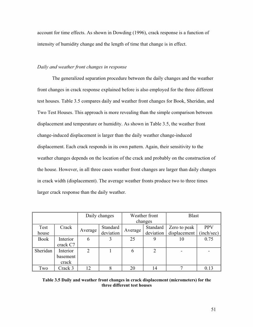
test houses. Table 3.5 compares daily and weather front changes for Book, Sheridan, and

Two Test Houses. This approach is more revealing than the simple comparison between

displacement and temperature or humidity. As shown in Table 3.5, the weather front

change-induced displacement is larger than the daily weather change-induced

displacement. Each crack responds in its own pattern. Again, their sensitivity to the

weather changes depends on the location of the crack and probably on the construction of

the house. However, in all three cases weather front changes are larger than daily changes

in crack width (displacement). The average weather fronts produce two to three times

larger crack response than the daily weather.

Daily changes Weather front changes

Blast

Test house

Crack Average Standard deviation Average Standard

deviation Zero to peak displacement

PPV (inch/sec)

Book Interior crack C7

6 3 25 9 10 0.75

Sheridan Interior basement

crack

2 1 6 2 - -

Two Crack 3 12 8 20 14 7 0.13

Table 3.5 Daily and weather front changes in crack displacement (micrometers) for the three different test houses

51

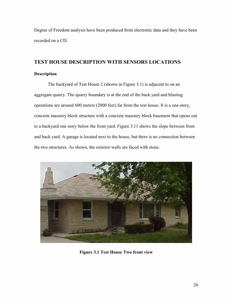
COMPARISON OF ENVIRONMENTAL EFFECTS AND BLAST EVENTS ON CRACK DISPLACEMENT For Test House Two For each blast event, the crack displacement “zero to peak” is collected for the

three crack sensors. After selecting the axis with the larger peak particle velocity, they are

named as follows. Each blast event has a unique name. The three or four first letters

indicate the month, the single digit before the dash symbolizes the year and finally the

two digits following the dash give the order of event in the month. For example, event

Oct0-13 is the thirtieth blast event that occurred in October 2000. According to the table

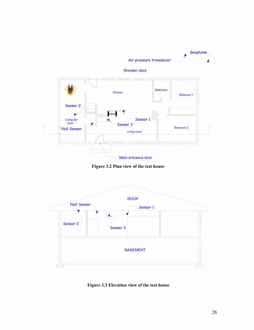
shown in the appendix A 3.17, the maximum crack response is given by Crack sensor 3,

which is located in the main entrance. Crack 2 reacts less than Crack 3 but more than

Crack 1, which shows the smallest response of the three.

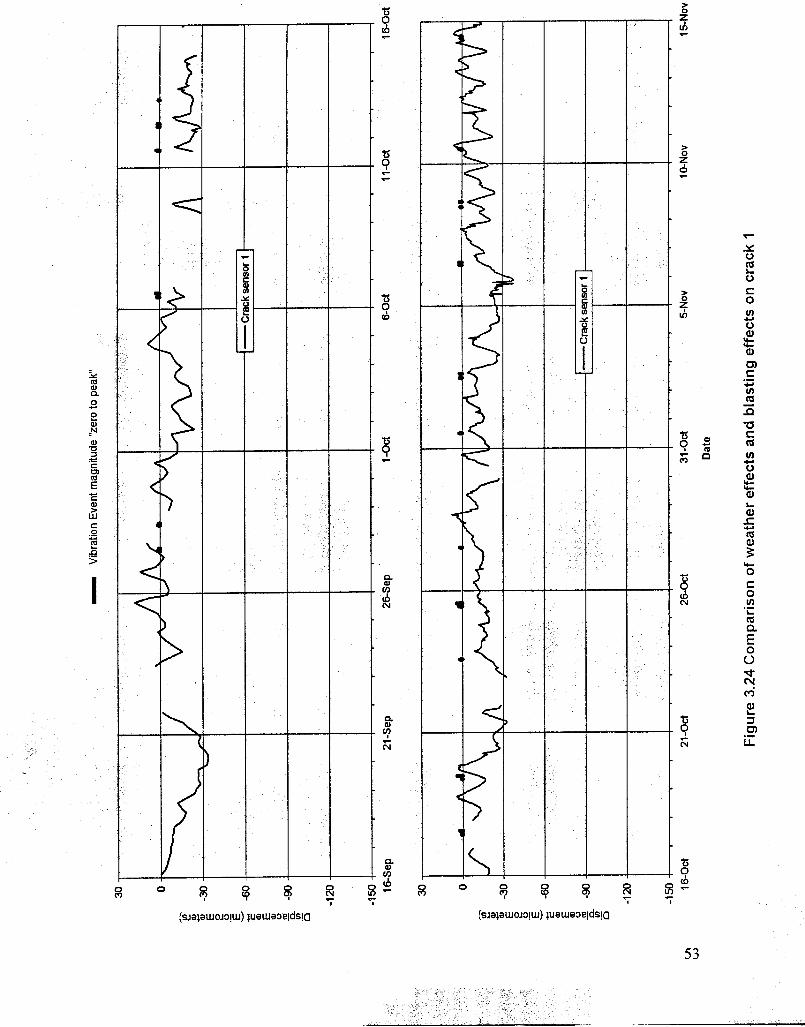
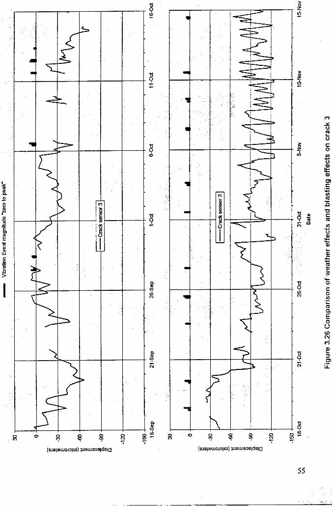
Comparisons of the environmental effects (from Figures 3.18, 3.19, and 3.20) and

the blast effects are presented in Figures 3.24, 3.25, 3.26 for each crack. Crack

displacements produced by a blast is insignificant compared to displacements produced

by environmental effects. This difference is most remarkable for the ceiling crack (2),

which is greatly affected by weather changes (see previous paragraph) but very little by

blasting.

52

For Book Test House and Test House Two

Two of the three test houses were subjected to blast events: Book and Two Test

Houses. The magnitude of crack displacement induced by blasting varied from house to

house. Figure 3.27 compares the maximum induced-blast crack displacement with that

caused by daily and the longer term weather front environmental changes (from Table

3.5) for the two different test houses

0

10

20

30

40

50

60

Test House 2 Crack3(0.13in/s)

Book Test HouseCrack7 (0.75in/s)

Cra

ck d

ispl

acem

ent (

mic

rom

eter

s)

Average weather front-induced displacement

blast-induced displacement

Average daily weather changes-induceddisplacement

0

10

20

30

40

50

60

Test House 2 Crack3 (0.13in/s)

Book Test HouseCrack7 (0.75in/s)

Cra

ck d

ispl

acem

ent (

mic

rom

eter

s)

Maximum weather front-induced displacement

blast-induced displacement

Maximum daily weather changes-induceddisplacement

Average

Maxima

Figure 3.27 Comparison of the maximum blast-induced displacement with maximum and average weather-induced crack displacement

In all cases, daily and longer term or weather front environmental changes greatly affect

crack displacement. Furthermore they produce larger crack displacements than does

blasting, even with relatively high ground motions. The weather front induced-crack

56

displacement is three and 2.5 times greater than the blast-induced displacements for Test

House Two and the Book Test House, respectively.

COMPARISON OF ENVIRONMENTAL EFFECTS AND HOUSEHOLD ACTIVITIES ON CRACK DISPLACEMENT For Test House Two

In terms of magnitude, crack displacements from household activity are not

significant compared to the daily environmentally-induced displacements. According to

Table 3.2, the maximum value “zero to peak” recorded was 3.5 micrometers for crack 3

while running in the living room. As shown in Table 3.3, the average daily changes for

Crack 3 is 12 micrometers and the maximum displacement from household activity for

Crack 3 is 3.5 micrometers as shown in Table 3.2.

Time histories of dynamic crack response to household events of door slamming

or running in the living room are compared to a typical blast response in Figures 3.28 and

3.29. This typical blast response was produced by ground motion with a single axis

maximum peak particle velocity of 0.09 inch per second. The door slam produces free

response after the single vertical pulse. Differences in the response and dominant

frequencies are discussed in detail below. The door slam produces single peaks at Crack

2 and 1 that are similar in magnitude to the 0.09 inch per second blast-induced ground

motion. Running in the living room produces similar peaks at Crack 1 as the blast, but

little to no response in Crack 2 located in the adjacent room ceiling.

Other time histories of household activity events are shown in appendices A 3.18

to A 3.21. These show the sensitivity of Crack 2 when the closet door is slammed and the

sensitivity of the geophones to near-by jumping or running.

57

For the three different test houses

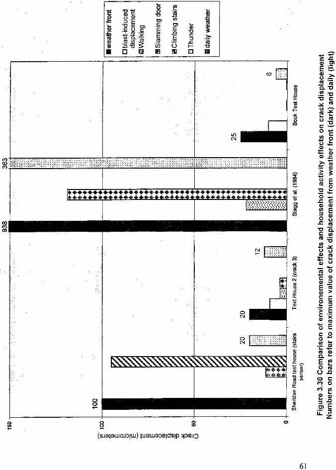
Figure 3.30 compares crack displacements produced by household activities with

weather effects for each test house and another study by Stagg et al. (1984). In the

Sheridan house, household activity events can produce greater crack displacement than

daily weather. However, these household activities produce less crack displacements than

weather front effects. Test house 2 shows that weather-front induced crack displacement

is at least ten times greater than the effect of slamming a door or running in the house for

the crack selected for the investigation. Test house 2 comparisons are based upon

response of crack 3. Even though for crack 3, household activities produce less effect

than blasting, environmental effects are by far more significant than blasting. Although

Stagg et al. (1984) results show far larger crack displacements from household activity

weather effects still dominate. Stagg et al. household activities were very close to the

gage position, which may account for the large magnitudes. In the Book Test House, the

household activity and thunder events produced displacements smaller than one

micrometer. However weather effects remain greater than blast vibrations effects on the

crack displacement.

All cracks in a house do not behave similary. Some of them respond more to the

weather changes and some more to household activities. However, as shown on Figure

3.30, weather changes tend to govern the crack displacement response.

60

HOUSE STRUCTURE RESPONSE

Twelve blast events have been selected to cover the span of excitation ground

motion magnitude and frequencies for the response study. Events showing free vibrations

have also been selected. Detailed time histories of these events are available in the

appendix. Table 3.6 indicates the use of each event selected. FFT refers to Fast Fourier

Transform and SDOF refers to Single Degree Of Freedom, which are explained further in

this section.

Event FFT Free vibration

SDOF and estimated displacement

Aug0-02 Aug0-03 Aug0-04 Sep0-02 Sep0-03 Oct0-02 Oct0-03 Oct0-09 Oct0-10 Oct0-12 Oct0-13 Oct0-14

Table 3.6 Twelve events selected to be analyzed

Estimation of the dominant frequency response of the house

Two methods are available to estimate the dominant frequency of the house. The

first involves comparison of the crack response with the ground motion time histories to

determine free response. Once ground motion excitation has ceased, the structure (and

crack) is free to respond at the natural frequency. Figure 3.31 represents an example of

free vibration in the crack response. It is also observed in the door slam response in

Figure 3.28.

62

Figure 3.31 Example of free vibration in the crack response

In this case, the dominant frequency response of the house, fs, is equal to:

HzT

f s 9sec110.0

11===

Five different events presented in appendices A 3.22 to A 3.26 showed free vibration.

Table 3.7 displays results from the calculation.

Crack sensor T (seconds) Fs (Hertz) Aug0-02 2 0.125 8 Sept0-02 1 0.078 13 Oct0-02 1 0.078 13 Oct0-09 3 0.120 8 Oct0-14 3 0.110 9

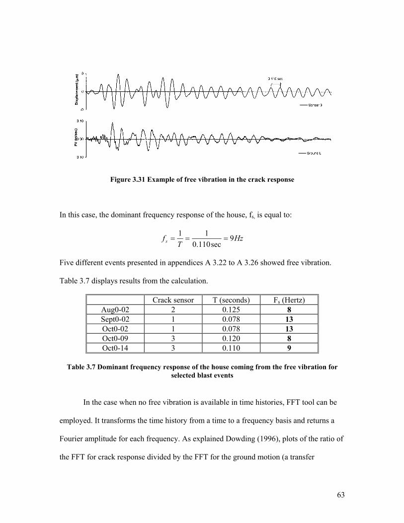
Table 3.7 Dominant frequency response of the house coming from the free vibration for

selected blast events

In the case when no free vibration is available in time histories, FFT tool can be

employed. It transforms the time history from a time to a frequency basis and returns a

Fourier amplitude for each frequency. As explained Dowding (1996), plots of the ratio of

the FFT for crack response divided by the FFT for the ground motion (a transfer

63

function), identifies the dominant frequency as that at which there is a maximum

amplification with a significant input amplitude. Time histories and FFT graphs are

contained in the appendices A 3.26 to A 3.33. Table 3.8 summarizes the results. Input

motion for the FFT transfer function were chosen at the basis of maximum response ratio.

While motions in all other axis were employed for Crack 1 and 3, only vertical motions

were employed for Crack 2.

Crack 1 Crack 2 Crack 3 Dominant frequency 12-13 Hz 8 or 11 Hz 8-9 Hz

Table 3.8 Dominant frequency for each crack using FFT method

SDOF analysis to estimate maximum displacement of the walls

As explained by Dowding (1996, Chapter 5), it is possible to estimate relative

wall displacement from pseudo velocity response of a single degree of freedom system to

the ground motion given the damping ratio and the system natural frequency. In this

study, the damping ratio is equal to 5 percent, which is typical and verified by analysis of

structural response to blast event oct0-02 in the transverse axis. The response spectrum

has been calculated with the ground motion time history from the axis with the maximum

peak particle velocity. The maximum displacement is read for a frequency equal to 11 Hz

for all cracks. The time histories employed are in appendices A 3.24, A 3.26, A 3.27, A

3.29, and A 3.33 to A 3.36.

64

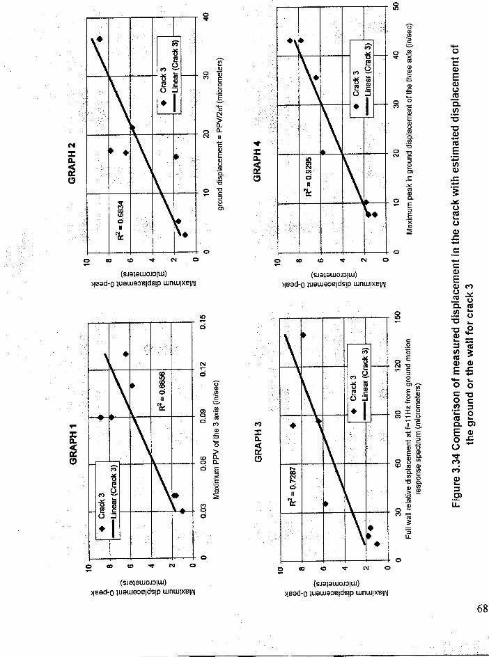
Comparison of estimated displacements and ground motion with actual crack displacements Four different methods of estimating crack response are compared with measured

crack displacement in Figures 3.32 to 3.34. They are as follows 1) Maximum peak

particle velocity of the three directions. 2) A sinusoidal estimate of the ground

displacement, taking into account the PPV and the frequency at which it occurs.3)

Relative displacement at 11 Hertz in the response spectrum of the particle velocity time

history of the ground showing the maximum PPV of the 3 directions. 4) Ground

displacement obtained by integrating the particle velocity of the time history showing the

maximum PPV.

Measured crack displacement are compared with these estimations of

displacement in graphs 1 through 4 for each crack. Details about the data are provided in

appendix A 3.37. The regression coefficients of the three cracks are shown in Table 3.9

for each approach.

Average correlation coefficient

Graph 1 Graph 2 Graph 3 Graph 4

Crack 1 0.4657 0.5749 0.6211 0.8357 Crack 2 0.7503 0.5778 0.4746 0.7009 Crack 3 0.6656 0.6834 0.7287 0.9295

Average for the 3 cracks 0.6272 0.6120 0.6081 0.8220

Table 3.9 Comparison of the correlation coefficients between the four different approaches

for Cracks 1, 2, and 3 in Test House Two to estimate wall displacement

65

The correlation coefficient is highest for the ground displacement by integration and

SDOF response. They are lower for the peak particle velocity and sinusoidal estimates of

peak ground displacement.

CONCLUSION

In Test House Two, daily and weekly weather related crack displacements are

greater than those produced by either type of dynamic event, household activities or

blasts. While the three cracks show a wide variation in response, all three show crack

displacements that far exceed the measured null sensor. They are so much larger that a

null sensor may not be needed in all cases. Frontal weather changes produce the greatest

crack response. While daily response is less, it is still greater than that produced by

vibration levels of up 0.13 inch per second. The natural frequency of the structure falls

within expected ranges. Finally, crack response shows greater correlation with ground

displacement obtained by integrating the excitation particle velocity time history and

single degree of freedom response.

69

CHAPTER 4

COMPARISON OF MICROMETER DISPLACEMENT SENSORS

INTRODUCTION

Long-term stability and resolution of five different micrometer displacement

sensors are compared in this chapter. Response of an LVDT sensor and two eddy current

sensors (Kaman 2400 and 2300 series) were reported by Siebert (2000). To those results

response of another eddy current sensor (Kaman 9000 series) and a fiberoptic sensor have

been added. All these sensors have been evaluated based on their resolution, range of

measurements, size, temperature sensitivity, electrical drift, and input and output

voltages.

70

MICROMETER DISPLACEMENT SENSORS REQUIREMENTS AND CRACK DISPLACEMENT DEFINITION Micrometer displacement requirements

Crack displacement sensors within the context of the Autonomous Crack

Comparometer (ACC) may be expected to perform for period up to one year. Thus, the

range of the sensor has to span the range of the change in crack displacement over one

year. Dowding (Chapter 13, 1996) measured a maximum displacement over a ten-month

test of 4 mils or 102 micrometers. Siebert (Chapter 5, 2000) recorded a maximum

displacement over a four-month period of 15 mils or 381 micrometers. Since the sensor

can be adjusted for unusual changes, the range does not have match an extreme such as

Siebert’s especially responsive crack. However, it should be expected that sensors should

be able to follow changes of plus or minus 200 micrometers without adjustment.

Another important technical requirement is the resolution of the sensor. Again,

according to the Dowding (1996) and Siebert (2000) experience, resolution must be at

least at a submicrometer scale in order to track daily temperature effects that might be on

the order of three micrometers. Thus minimum resolution of 0.1 micrometers or 0.004

mils is preferred. The resolution depends on the range of the sensor, the larger the range,

the less the resolution. Thus range and resolution must be considered together. Resolution

is also dependent upon the A/D converter resolution. A 12-bit A/D converter, which is

capable of 4096 subdivisions, can achieve a resolution of (400/4096) = 0.1 micrometer

for a sensor with a plus or minus 200 micrometers.

71

Crack displacement definition

The crack width is not really measured, but rather the variations of the crack

width as shown in Figure 4.1. The “change in crack width” will hereinafter be defined as

crack displacement. By measuring the crack displacement instead of the crack width, it is

possible to mount the sensor probe and the target away from the exact sides of the crack.

Typical Crack

Total Crack Width

Change in Crack Width

Figure 4.1 Crack displacement definition (Siebert, 2000)

TEST DESCRIPTION

Comparison of sensor response with theoretical displacement

In order to quantify the effects of electrical drift and cyclical temperature changes,

sensors and electronics were subjected to a long-term environmentally variable test. The

sensors were mounted on an aluminum block of a known coefficient of thermal

72

expansion (CTE). Thermocouples (as shown on Figure 4.2) were mounted on the block to

determine the current temperature. All sensors and electronics together were subjected to

temperature that cyclically ranged between 5 to 35 degrees Celsius (41 to 95 degrees

Fahrenheit) during daily temperature changes. Readings were taken every five minutes

during the test period. The electronics and the sensors followed the same temperatures

during the test by virtue of their identical location. Sensor response is evaluated by

comparison with theoretical response of the aluminum. The theoretical displacement was

computed from the known temperature variation and CTE by multiplying the CTE by the

initial distance between the two brackets by the temperature changes. The CTE for the

aluminum is equal to 0.02358 mils per degree Celsius per inch.

Mounting

The sensor is mounted on an aluminum plate, as shown on Figure 4.2. This plate

measures 10 inches by 7 inches. Two aluminum brackets, details of which are shown in

Figure 4.3, are epoxyed to the plate. As it is shown on Figure 4.2, one supports the sensor

probe and the other is a target to for the sensor. The initial distance between the two

aluminum brackets is 0.25 inch (6 mm) for LVDT and 0.75 inch (19 mm) for the eddy

current sensors. The initial distance between the sensor tip and the target for the eddy

current sensors is 10 mils (254 micrometers)

73

Thermocouple

Figure 4.2 Sensor mounted an a aluminum plate between two aluminum brackets

Figure 4.3 Elevation, top, plan, and 3D views of the aluminum bracket receiving the sensor. Dimensioning is in inches

74

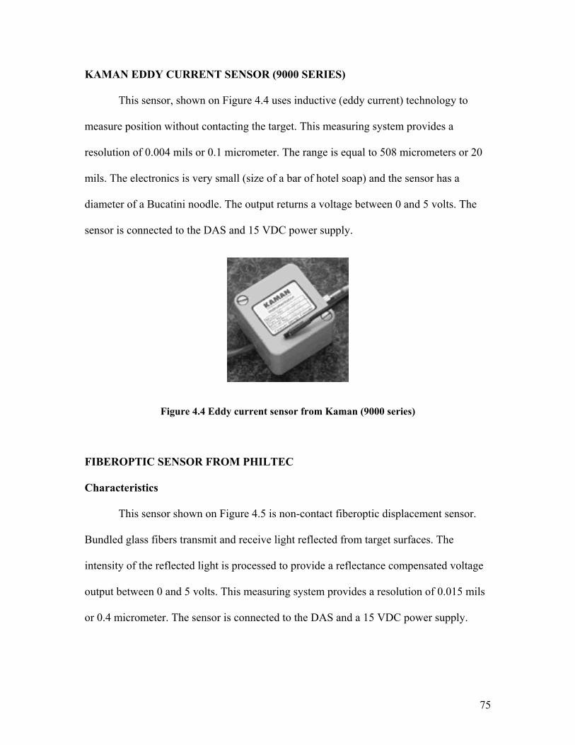
KAMAN EDDY CURRENT SENSOR (9000 SERIES)

This sensor, shown on Figure 4.4 uses inductive (eddy current) technology to

measure position without contacting the target. This measuring system provides a

resolution of 0.004 mils or 0.1 micrometer. The range is equal to 508 micrometers or 20

mils. The electronics is very small (size of a bar of hotel soap) and the sensor has a

diameter of a Bucatini noodle. The output returns a voltage between 0 and 5 volts. The

sensor is connected to the DAS and 15 VDC power supply.

Figure 4.4 Eddy current sensor from Kaman (9000 series)

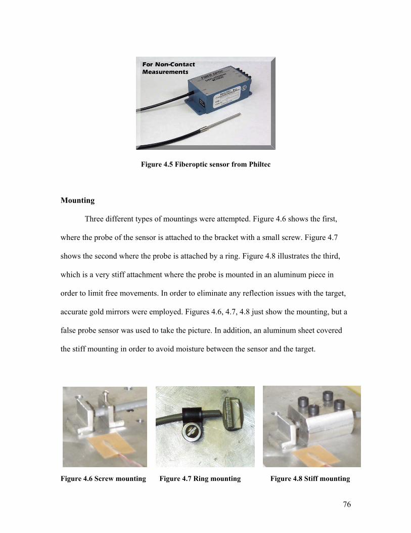
FIBEROPTIC SENSOR FROM PHILTEC

Characteristics

This sensor shown on Figure 4.5 is non-contact fiberoptic displacement sensor.

Bundled glass fibers transmit and receive light reflected from target surfaces. The

intensity of the reflected light is processed to provide a reflectance compensated voltage

output between 0 and 5 volts. This measuring system provides a resolution of 0.015 mils

or 0.4 micrometer. The sensor is connected to the DAS and a 15 VDC power supply.

75

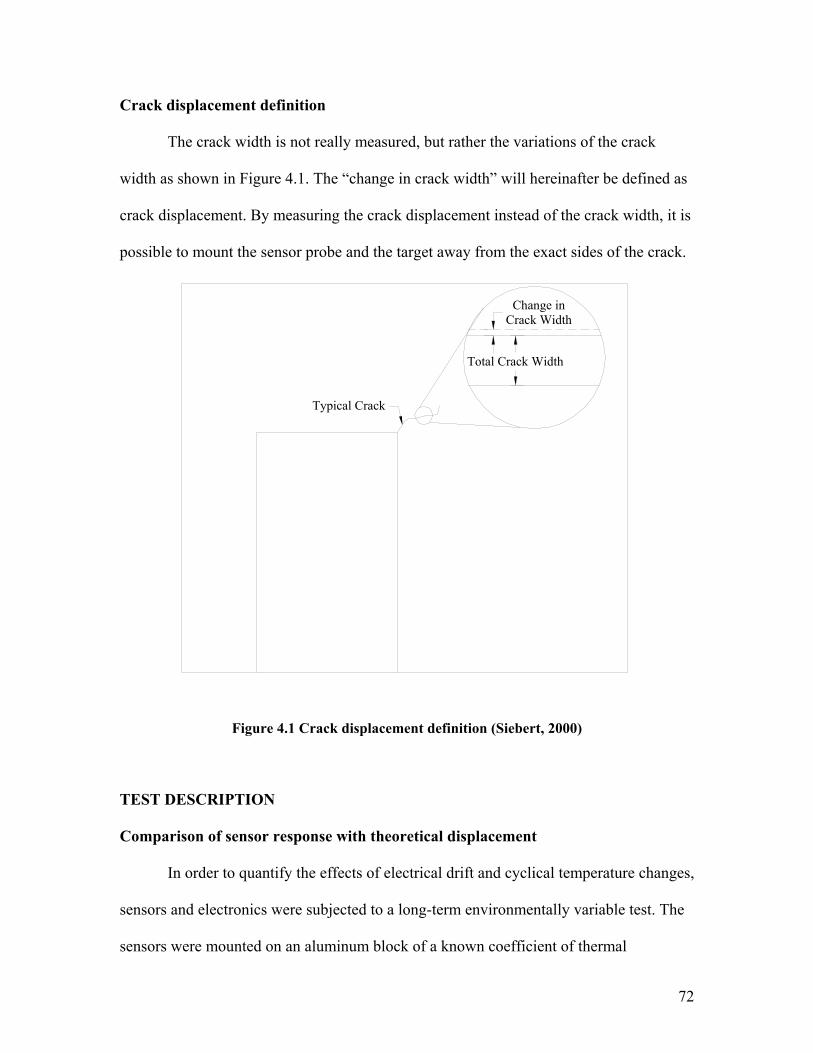
Figure 4.5 Fiberoptic sensor from Philtec

Mounting

Three different types of mountings were attempted. Figure 4.6 shows the first,

where the probe of the sensor is attached to the bracket with a small screw. Figure 4.7

shows the second where the probe is attached by a ring. Figure 4.8 illustrates the third,

which is a very stiff attachment where the probe is mounted in an aluminum piece in

order to limit free movements. In order to eliminate any reflection issues with the target,

accurate gold mirrors were employed. Figures 4.6, 4.7, 4.8 just show the mounting, but a

false probe sensor was used to take the picture. In addition, an aluminum sheet covered

the stiff mounting in order to avoid moisture between the sensor and the target.

Figure 4.6 Screw mounting

Figure 4.7 Ring mounting

Figure 4.8 Stiff mounting

76

TEST RESULTS FOR THE FIBEROPTOC SENSOR

This test is treated separately because, as shown in appendix A 4.1, it does not

meet the requirements to measure micrometer crack displacement in long-term

conditions. For the screw mounting, the graphs shows that there is an attachment problem

according to the gap width values, which are reasonable during the first hours of the test,

but are too low afterwards. It seems that the attachment may have been too loose. For the

ring mounting, there are some irregularities in the early morning probably because of the

dew. For the stiff mounting, the graph is smoother, so the moisture problem seems to be

solved. However, the attachment is too stiff or too thermally massive because there is no

peak in the displacement.

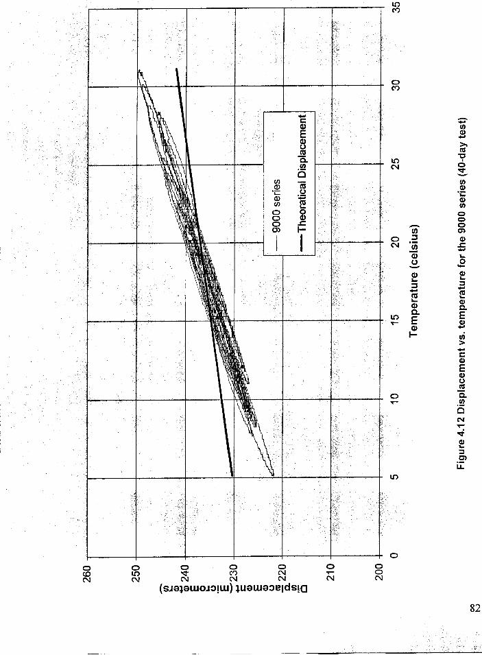
Thus, the precision of the optical sensor is affected by moisture and mounting

stiffness. No mounting has been found to produce variations in measured width similar to

those calculated from the aluminum CTE, which led to the daily loop shown in Figure

4.12 for the Kaman gages.

DISPLACEMENT VERSUS TEMPERATURE

Evaluation of the four other sensors is based upon graphical comparison of

displacement versus temperature as shown on Figures 4.9, 4.10, 4.11, and 4.12 for the

LVDT and the 2400, 2300, and 9000 series sensors. Every five minutes, displacement is

plotted on the same scale versus temperature for each sensor. The theoretical

displacement (from CTE) is also displayed on each graph for comparison. Sensor

response appears to be cyclic with variable hysteresis.

77

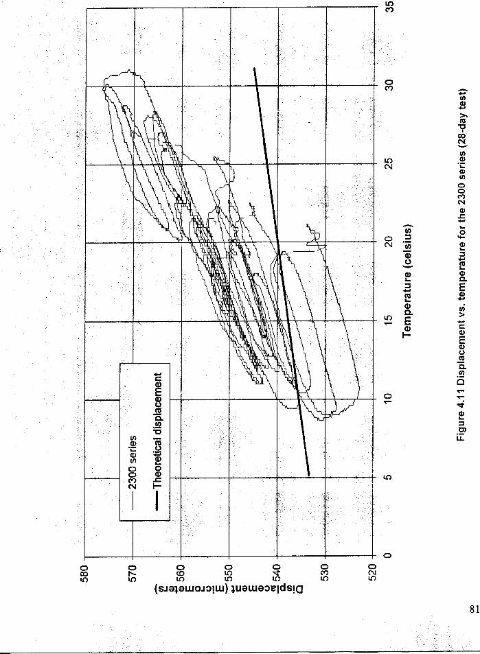
Ideally, the best correlation would be a linear relationship between the theoretical

displacement values and the measured displacement values. Figure 4.11 clearly shows

that the sensor behavior can be separated in two parts: electrical drift and daily hysteresis.

By looking at a one-day cycle the effect of electronic drift is removed because the

electronic drift is a long-term effect, and should have a minimal effect on a one-day

cycle.

The LVDT measured displacements follow the theoretical displacement most

closely of all the sensors and the Kaman 9000 is the next closest follower. The average

slope of the theoretical and measured displacements varies. This slope is a function of

mounting details. Its effect is taken into account in the conversion of sensor output to

displacement.

78

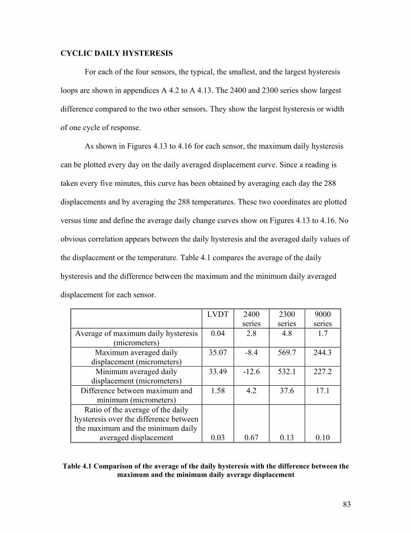
CYCLIC DAILY HYSTERESIS

For each of the four sensors, the typical, the smallest, and the largest hysteresis

loops are shown in appendices A 4.2 to A 4.13. The 2400 and 2300 series show largest

difference compared to the two other sensors. They show the largest hysteresis or width

of one cycle of response.

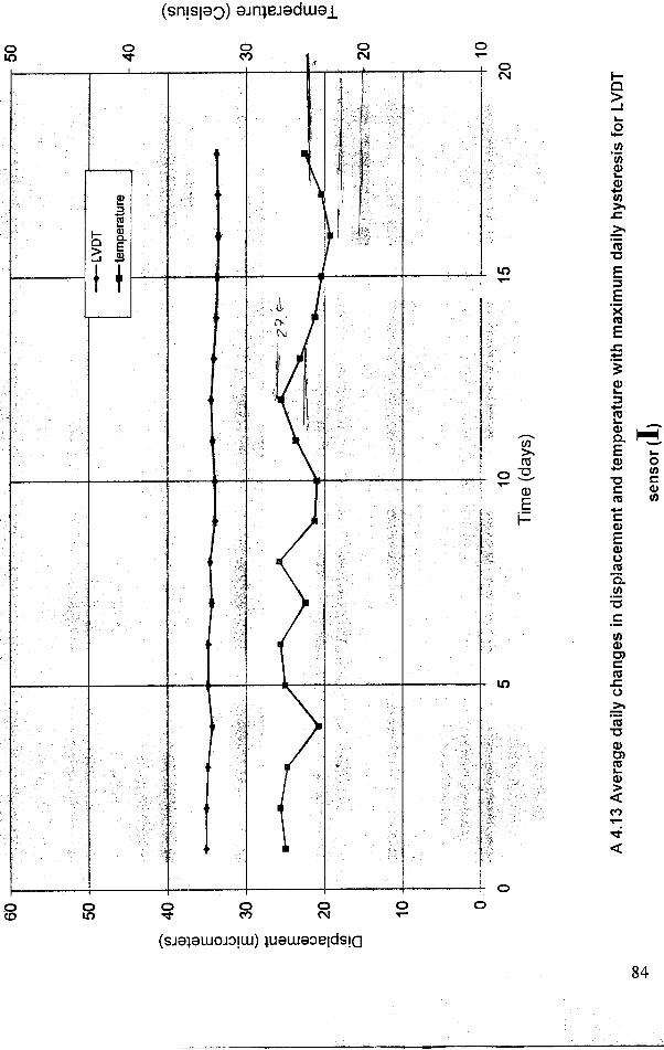
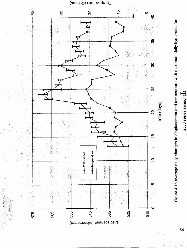
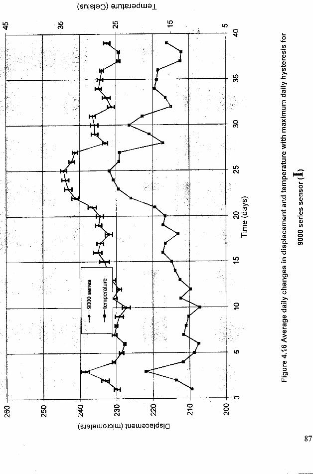
As shown in Figures 4.13 to 4.16 for each sensor, the maximum daily hysteresis

can be plotted every day on the daily averaged displacement curve. Since a reading is

taken every five minutes, this curve has been obtained by averaging each day the 288

displacements and by averaging the 288 temperatures. These two coordinates are plotted

versus time and define the average daily change curves show on Figures 4.13 to 4.16. No

obvious correlation appears between the daily hysteresis and the averaged daily values of

the displacement or the temperature. Table 4.1 compares the average of the daily

hysteresis and the difference between the maximum and the minimum daily averaged

displacement for each sensor.

LVDT 2400 series

2300 series

9000 series

Average of maximum daily hysteresis (micrometers)

0.04 2.8 4.8 1.7

Maximum averaged daily displacement (micrometers)

35.07 -8.4 569.7 244.3

Minimum averaged daily displacement (micrometers)

33.49 -12.6 532.1 227.2

Difference between maximum and minimum (micrometers)

1.58 4.2 37.6 17.1

Ratio of the average of the daily hysteresis over the difference between the maximum and the minimum daily

averaged displacement 0.03 0.67 0.13 0.10

Table 4.1 Comparison of the average of the daily hysteresis with the difference between the maximum and the minimum daily average displacement

83

The LVDT sensor has the least thermal hysteresis whereas the 2400 series sensor

produces the more hysteresis. If the hysteresis is normalized by dividing it by the average

displacement, the LVDT still induces the least. However, the 9000 series offers a

reasonable alternative.

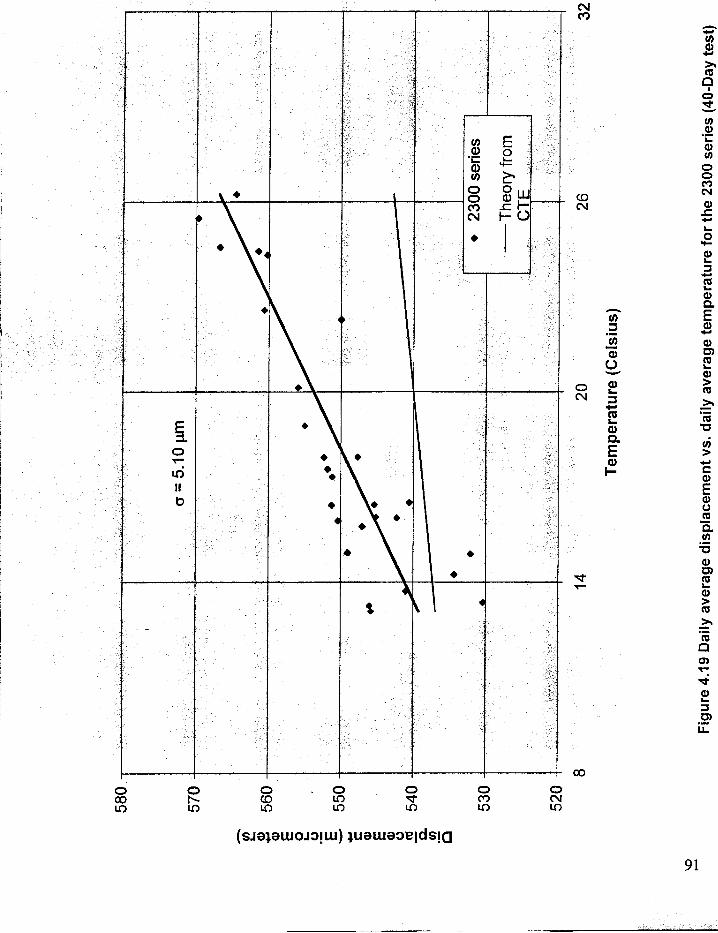
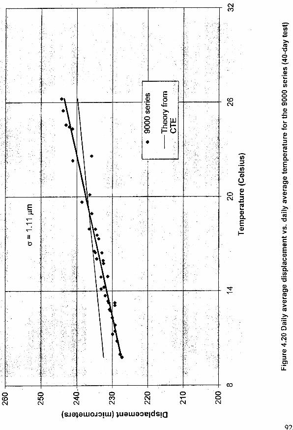
LONG-TERM ELECTRICAL DRIFT

The electrical drift characterizes the long-term behavior of the sensor. The

electrical drift can be isolated by plotting the daily average displacement versus the daily

average temperature as a single point as shown on Figures 4.17, 4.18, 4.19, and 4.20 for

the LVDT and 2400, 2300, and 9000 series respectively. This averaging approach

discounts the daily hysteresis and enables a focus on the electrical drift. The correlation

of the average daily displacement temperature relationship with its mean linear trend

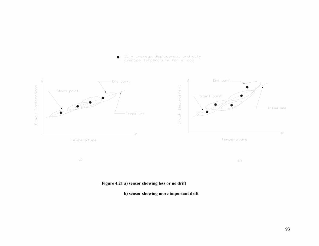
describes the degree of drift. As shown in Figures 4.21, sensor whose average response is

closer to the mean trend (a) would show less drift that with case (b). Table 4.2 compares

the standard deviation of the average daily displacement and temperature relationship

from the best linear trend line passing through the data series (from Figures 4.17 to 4.20).

LVDT 2400 series 2300 series 9000 series Standard deviation σ

(micrometers) 0.25 0.86 5.10 1.11

Table 4.2 Comparison for each sensor of standard deviation of the average displacement

and temperature relationship from the best linear trend line

88

Figure 4.21 a) sensor showing less or no drift

b) sensor showing more important drift

93

Without considering the daily hysteresis, the 2300 series produces the largest scatter or

standard deviation (drift) as seen on the Figure 4.19. The LVDT, 2400 and 9000 series

involve similar standard deviations (drift). However, the 2400 series has large hysteresis.

Comparison of Figures 4.17, 4.18, 4.19, and 4.20 shows that the mean trend line

do not have the same slope as the theoretical. This difference may result from a number

of systematic factors from the mounting but is eliminated through the conversion of

transducer response to displacement based upon these comparisons

CONCLUSION

The LVDT and the Kaman 9000 appear to be the best over-all micrometer

displacement sensors. Of the five sensors tested, it appears that the fiberoptic sensor

cannot not meet project needs because of mounting and moisture issues. The 2300 and

2400 series show unacceptable drift and hysteresis compared to the LVDT sensor and the

9000 series sensors. The eddy current sensor series 9000 from Kaman is small, easy to

mount and produces an acceptable hysteresis value, and has an acceptably small drift.

94

CHAPTER 5

CONCLUSIONS AND FUTURE WORK

Summary

Public concern over the possibility of construction vibration-induced cracking led

to the creation of a new approach to vibration monitoring, an Autonomous Crack

Comparometer (ACC). This system automatically compares long-term weather-induced

micrometer changes in crack opening with those produced by household activities and

ground motion. This comparison is displayed in real time via the Internet without human

interaction. The first step of developing equipment and software necessary for this system

was fully described by Siebert (2000).

The thesis describes the second phase of development of the ACC system to

incorporate measurements of ground motions and add several changes in the autonomous

operation. In order to obtain the ground motion and air blast data, four additional

transducers have been added. There are now a total of ten channels of data autonomously

collected and comparatively displayed by ACC. The web page has been fully developed

and now dynamic blast effects are compared with long-term effects. Data are password

95

protected. Finally, new data acquisition system software has been installed that allows

direct modem communication.

Conclusions

The ACC installed in Test House Two allowed measurements that verified past

experience that daily and weekly weather related crack displacements are greater than

those produced by dynamic events, whether they are household activities or blasts.

Frontal (weekly) weather changes produce the greatest crack response. Measurements

with the null sensor may not be needed because crack displacements are much larger than

null sensor displacements.

Five different crack displacement sensors were evaluated to determine magnitude

of thermal hysteresis and long-term electronic drift. Robust sensors are needed for this

application. The eddy current sensor (9000 series) offers a good compromise. It is small,

easy to mount, and provides an acceptable hysteresis value, as well as linear response.

The LVDT also is acceptable.

Future work

The next phase (III) ACC system should trigger the data acquisition system with

household activity events or with thunder event for additional automatic comparison. The

first step will be to set trigger thresholds on crack displacement sensors and on the air

pressure transducer. The second step will be to develop logical filters in the Java

programs in order to distinguish a household activity from a blast vibration event.

96

The web should also present time histories of crack response for each vibration

event. At first these time histories will be provided by a look up table. Eventually it is

hoped that the time histories can be accessed by clicking on a blast point on the graph

comparing long-term crack displacement with that produced by blasting.

Finally, the automate tasks will be modified with the professional version of

Automate (Unisyn, version 4.5, 1999). This version will help to improve the reliability of

the data transfer from the DAS to the Polling computer.

97

REFERENCES

Dowding, C. H. (1996) Construction Vibrations, Prentice Hall, Upper Saddle River, New Jersey, Chapter 13, "Comparison of Environmental and Vibration-Induced Crack Movement".

Dowding, Charles H. (2000), Personal Communication. Professor, Department of

Civil Engineering Northwestern University, Evanston IL. Kaman Instrumentation Corporation (2000). SMU-9000 User Manual. 3450 North

Nevada Avenue P.O. Box 33010. Geosonics Inc. (2000). Calibration Data for supplied Geophone P.O. Box 779

Warrendale, PA 15095. Kosnik D. (2000), Personal Communication, Student, Department of Electrical and

Computer Engineering, Northwestern University, Evanston, IL. Omega Engineering, Inc. (1989). Omega Manual Model HX93 Relative Humidity

and Temperature Transmitter: Operations Manual. One Omega Drive Stamford, CT.

Sensym Inc. (1988) Sensym manual for 142SC Series 1804 Mc Carthy Blvd Milpitas,

CA 95035. Siebert, D. (2000), Autonomous Crack Comparometer. Master of Science Thesis,

Department of Civil Engineering, Northwestern University, Evanston, IL.

Siebert, D. (2000), Appendixes for Autonomous Crack Comparometer Phase I. Internal Report for Infrastructure Technology Institute, Northwestern University, Evanston, IL.

Somat Corporation, (1999), “EASE Ver 3.03.10” SoMat Corporation 702 West

Killarney Urbana, IL. Somat Corporation, (1999), “WinTCS Ver. 2.0.1 “ SoMat Corporation 702 West

Killarney Urbana, IL.

98

Symantec Corporation, (2000), “PcAnywhere Ver. 9.2.1” Symantec Corporate Offices, 20330 Stevens Creek Blvd., Cupertino, CA.

Unisyn Software, LLC (2000), “AutoMate, Ver. 4.5” 3440 Wilshire Boulevard Suite

910, Los Angeles, CA.

99

Date post:	11-Oct-2018
Category:	Documents
Upload:	phungkhanh
View:	214 times
Download:	0 times

NORTHWESTERN UNIVERSITY · I would like to gratefully acknowledge Mr. Daniel Aucouturier,...

Documents