Page 1
Priorsforthelongrun
Giannone,Lenza,Prim iceri Priors for the long run
Domenico GiannoneNewYorkFed
MicheleLenzaEuropeanCentralBank
GiorgioPrimiceriNorthwesternUniversity
9th ECB Workshop on Forecasting TechniquesJune3,2016
Page 2
Giannone,Lenza,Prim iceri Priors for the long run
Whatwedo
n ProposeaclassofpriordistributionsforVARsthatdisciplinethelong-runimplicationsofthemodel
Priorsforthelongrun
Page 3
Giannone,Lenza,Prim iceri Priors for the long run
Whatwedo
n ProposeaclassofpriordistributionsforVARsthatdisciplinethelong-runimplicationsofthemodel
Priorsforthelongrun
n PropertiesØ BasedonmacroeconomictheoryØ Conjugateà Easy toimplement andcombinewithexistingpriors
n Performwell inapplicationsØ Good(long-run)forecastingperformance
Page 4
Giannone,Lenza,Prim iceri Priors for the long run
Outline
n Aspecificpathologyof(flat-prior)VARsØ Toomuchexplanatorypowerofinitialconditionsanddeterministic trendsØ Sims(1996and2000)
n PriorsforthelongrunØ IntuitionØ Specificationandimplementation
n Alternativeinterpretationsandrelationwiththeliterature
n Application:macroeconomicforecasting
Page 5
Giannone,Lenza,Prim iceri Priors for the long run
Simpleexample
n AR(1):
€
yt = c + ρyt−1 +ε t
Page 6
Giannone,Lenza,Prim iceri Priors for the long run
Simpleexample
n AR(1):
n Iteratebackwards:
€
yt = c + ρyt−1 +ε t
€
yt = ρ t y0 + ρ jcj=0
t−1∑ + ρ jε t− jj=0
t−1∑
Page 7
Giannone,Lenza,Prim iceri Priors for the long run
Simpleexample
n AR(1):
n Iteratebackwards:
➠ModelseparatesobservedvariationofthedataintoØ DC:deterministic component,predictablefromdataattime0Ø SC:unpredictable/stochastic component
€
yt = c + ρyt−1 +ε t
€
yt = ρ t y0 + ρ jcj=0
t−1∑ + ρ jε t− jj=0
t−1∑
SCDC
Page 8
Giannone,Lenza,Prim iceri Priors for the long run
Simpleexample
n AR(1):
n Iteratebackwards:
➠ModelseparatesobservedvariationofthedataintoØ DC:deterministic component,predictablefromdataattime0Ø SC:unpredictable/stochastic component
n Ifρ =1,DCisasimplelineartrend:
€
yt = c + ρyt−1 +ε t
€
yt = ρ t y0 + ρ jcj=0
t−1∑ + ρ jε t− jj=0
t−1∑
€
DC = y0 + c⋅ t
SCDC
Page 9
Giannone,Lenza,Prim iceri Priors for the long run
Simpleexample
n AR(1):
n Iteratebackwards:
➠ModelseparatesobservedvariationofthedataintoØ DC:deterministic component,predictablefromdataattime0Ø SC:unpredictable/stochastic component
n Ifρ =1,DCisasimplelineartrend:
n Otherwisemorecomplex:
€
yt = c + ρyt−1 +ε t
€
yt = ρ t y0 + ρ jcj=0
t−1∑ + ρ jε t− jj=0
t−1∑
€
DC = y0 + c⋅ t
€
DC =c
1− ρ+ ρ t y0 −
c1− ρ
$
% &
'
( )
SCDC
Page 10
Giannone,Lenza,Prim iceri Priors for the long run
Pathologyof(flat-prior)VARs(Sims,1996and2000)
n OLS/MLEhasatendencyto“use”thecomplexityofdeterministiccomponentstofitthelowfrequencyvariationinthedata
n Possiblebecauseinferenceistypicallyconditionalony0Ø Nopenalizationforparameterestimates ofimplyingsteadystates ortrendsfar
awayfrominitialconditions
Page 11
Giannone,Lenza,Prim iceri Priors for the long run
DeterministiccomponentsinVARs
n ProblemmoreseverewithVARsØ implieddeterministic component ismuchmorecomplexthaninAR(1)case
Page 12
Giannone,Lenza,Prim iceri Priors for the long run
DeterministiccomponentsinVARs
n ProblemmoreseverewithVARsØ implieddeterministic component ismuchmorecomplexthaninAR(1)case
n Example:7-variableVAR(5)withquarterlydataonØ GDPØ ConsumptionØ InvestmentØ RealWagesØ HoursØ InflationØ Federalfundsrate
n Sample:1955:I– 1994:IV
n FlatorMinnesotaprior
Page 13
Giannone,Lenza,Prim iceri Priors for the long run
“Over-fitting”ofdeterministiccomponentsinVARs
1960 1980 2000
5.55.65.75.85.9
66.16.26.36.4
GDP
1960 1980 20003.9
44.14.24.34.44.54.64.7
Investment
1960 1980 2000
-0.65
-0.6
-0.55
-0.5
Hours
1960 1980 2000
-1.7-1.65
-1.6-1.55
-1.5-1.45
-1.4-1.35
-1.3-1.25
Investment-to-GDP ratio
1960 1980 2000-0.015
-0.01-0.005
00.005
0.010.015
0.020.025
Inflation
1960 1980 2000
-0.01
0
0.01
0.02
0.03
0.04
Interest rate
Data Flat MN PLR
Page 14
Giannone,Lenza,Prim iceri Priors for the long run
“Over-fitting”ofdeterministiccomponentsinVARs
1960 1980 2000
5.55.65.75.85.9
66.16.26.36.4
GDP
1960 1980 20003.9
44.14.24.34.44.54.64.7
Investment
1960 1980 2000
-0.65
-0.6
-0.55
-0.5
Hours
1960 1980 2000
-1.7-1.65
-1.6-1.55
-1.5-1.45
-1.4-1.35
-1.3-1.25
Investment-to-GDP ratio
1960 1980 2000-0.015
-0.01-0.005
00.005
0.010.015
0.020.025
Inflation
1960 1980 2000
-0.01
0
0.01
0.02
0.03
0.04
Interest rate
Data Flat MN PLR
Page 15
Giannone,Lenza,Prim iceri Priors for the long run
Pathologyof(flat-prior)VARs(Sims,1996and2000)
n OLS/MLEhasatendencyto“use”thecomplexityofdeterministiccomponentstofitthelowfrequencyvariationinthedata
n Possiblebecauseinferenceistypicallyconditionalony0Ø Nopenalizationforparameterestimates ofimplyingsteadystates ortrendsfar
awayfrominitialconditions
➠Flat-priorVARsattributean(implausibly) largeshareofthelowfrequencyvariationinthedatatodeterministiccomponents
Page 16
Giannone,Lenza,Prim iceri Priors for the long run
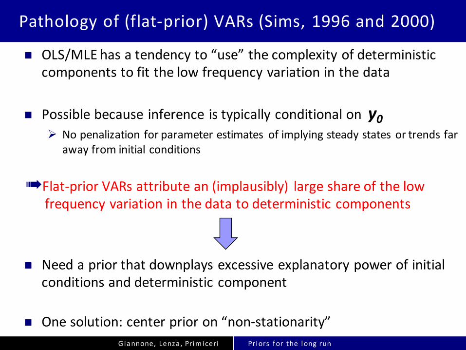
Pathologyof(flat-prior)VARs(Sims,1996and2000)
n OLS/MLEhasatendencyto“use”thecomplexityofdeterministiccomponentstofitthelowfrequencyvariationinthedata
n Possiblebecauseinferenceistypicallyconditionalony0Ø Nopenalizationforparameterestimates ofimplyingsteadystates ortrendsfar
awayfrominitialconditions
➠Flat-priorVARsattributean(implausibly) largeshareofthelowfrequencyvariationinthedatatodeterministiccomponents
n Needapriorthatdownplaysexcessiveexplanatorypowerofinitialconditionsanddeterministiccomponent
n Onesolution:centerprioron“non-stationarity”
Page 17
Giannone,Lenza,Prim iceri Priors for the long run
Outline
n Aspecificpathologyof(flat-prior)VARsØ Toomuchexplanatorypowerofinitialconditionsanddeterministic trendsØ Sims(1996and2000)
n PriorsforthelongrunØ IntuitionØ Specificationandimplementation
n Alternativeinterpretationsandrelationwiththeliterature
n Application:macroeconomicforecasting
Page 18
Giannone,Lenza,Prim iceri Priors for the long run
Priorforthelongrun
€
VAR(1) : yt = c + Byt−1 +ε t , ε t ~ N 0,Σ( )
Page 19
Giannone,Lenza,Prim iceri Priors for the long run
Priorforthelongrun
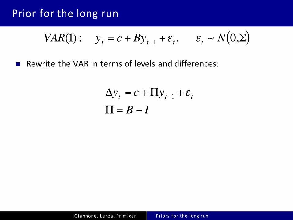
n RewritetheVARintermsoflevelsanddifferences:
€
VAR(1) : yt = c + Byt−1 +ε t , ε t ~ N 0,Σ( )
€
Δyt = c +Πyt−1 +ε tΠ = B − I
Page 20
Giannone,Lenza,Prim iceri Priors for the long run
Priorforthelongrun
n RewritetheVARintermsoflevelsanddifferences:
n Priorforthelongrun prioroncenteredat0
€
VAR(1) : yt = c + Byt−1 +ε t , ε t ~ N 0,Σ( )
€
Δyt = c +Πyt−1 +ε tΠ = B − I
€
Π
Page 21
Giannone,Lenza,Prim iceri Priors for the long run
Priorforthelongrun
n RewritetheVARintermsoflevelsanddifferences:
n Priorforthelongrun prioroncenteredat0
n Standardapproach(DLS,SZ,andmanyfollowers)Ø Pushcoefficientstowardsallvariablesbeingindependentrandomwalks
€
VAR(1) : yt = c + Byt−1 +ε t , ε t ~ N 0,Σ( )
€
Δyt = c +Πyt−1 +ε tΠ = B − I
€
Π
Page 22
Giannone,Lenza,Prim iceri Priors for the long run
Priorforthelongrun
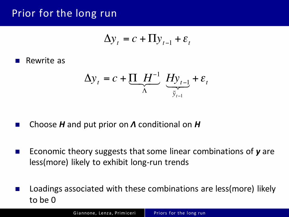
n Rewriteas
€
Δyt = c +Πyt−1 +ε t
€
Δyt = c +Π H −1
Λ! " # Hyt−1
˜ y t−1
! " # +ε t
Page 23
Giannone,Lenza,Prim iceri Priors for the long run
Priorforthelongrun
n Rewriteas
n ChooseH andputprioronΛ conditionalonH
€
Δyt = c +Πyt−1 +ε t
€
Δyt = c +Π H −1
Λ! " # Hyt−1
˜ y t−1
! " # +ε t
Page 24
Giannone,Lenza,Prim iceri Priors for the long run
Priorforthelongrun
n Rewriteas
n ChooseH andputprioronΛ conditionalonH
n Economictheorysuggeststhatsomelinearcombinationsofy areless(more)likelytoexhibitlong-runtrends
€
Δyt = c +Πyt−1 +ε t
€
Δyt = c +Π H −1
Λ! " # Hyt−1
˜ y t−1
! " # +ε t
Page 25
Giannone,Lenza,Prim iceri Priors for the long run
Priorforthelongrun
n Rewriteas
n ChooseH andputprioronΛ conditionalonH
n Economictheorysuggeststhatsomelinearcombinationsofy areless(more)likelytoexhibitlong-runtrends
n Loadingsassociatedwiththesecombinationsareless(more)likelytobe0
€
Δyt = c +Πyt−1 +ε t
€
Δyt = c +Π H −1
Λ! " # Hyt−1
˜ y t−1
! " # +ε t
Page 26
Giannone,Lenza,Prim iceri Priors for the long run
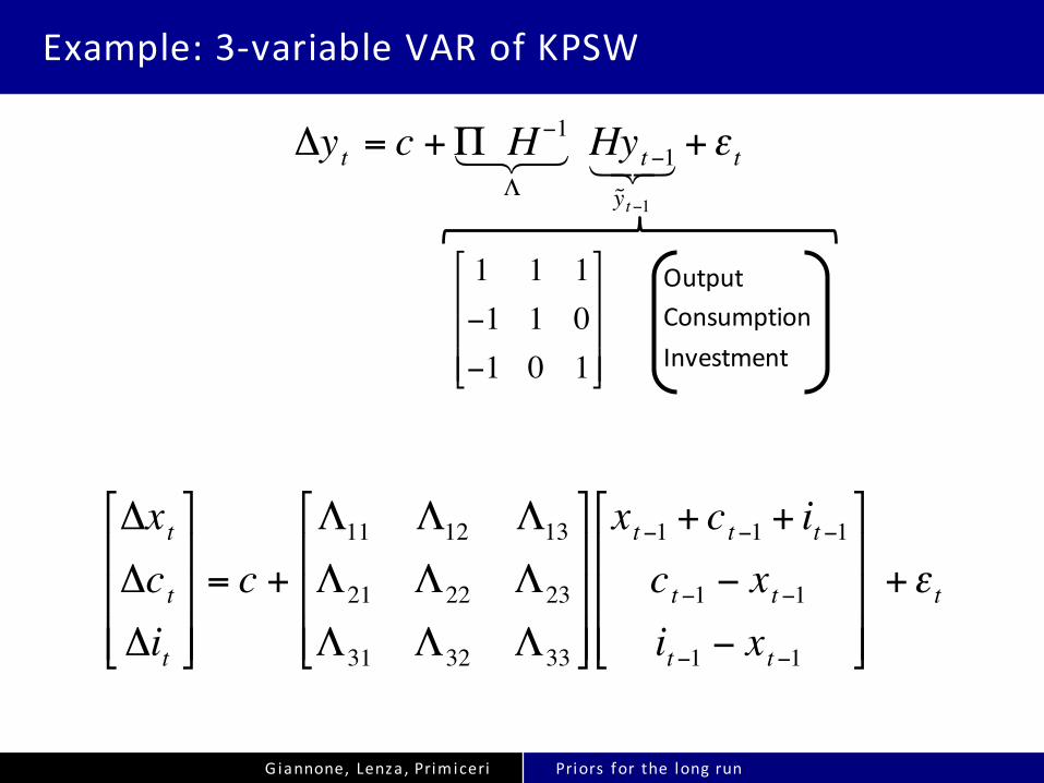
Example:3-variableVARofKPSW
OutputConsumptionInvestment
€
Δyt = c +Π H −1
Λ! " # Hyt−1
˜ y t−1
! " # +ε t
€
1 1 1−1 1 0−1 0 1
#
$
% % %
&
'
( ( (
Page 27
Giannone,Lenza,Prim iceri Priors for the long run
Example:3-variableVARofKPSW
OutputConsumptionInvestment
€
ΔxtΔctΔit
#
$
% % %
&
'
( ( (
= c +
Λ11 Λ12 Λ13
Λ21 Λ22 Λ23
Λ31 Λ32 Λ33
#
$
% % %
&
'
( ( (
xt−1 + ct−1 + it−1
ct−1 − xt−1
it−1 − xt−1
#
$
% % %
&
'
( ( ( +ε t
€
Δyt = c +Π H −1
Λ! " # Hyt−1
˜ y t−1
! " # +ε t
€
1 1 1−1 1 0−1 0 1
#
$
% % %
&
'
( ( (
Page 28
Giannone,Lenza,Prim iceri Priors for the long run
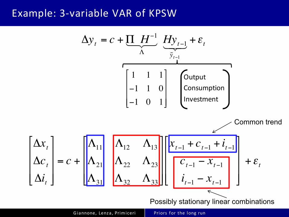
Example:3-variableVARofKPSW
OutputConsumptionInvestment
€
ΔxtΔctΔit
#
$
% % %
&
'
( ( (
= c +
Λ11 Λ12 Λ13
Λ21 Λ22 Λ23
Λ31 Λ32 Λ33
#
$
% % %
&
'
( ( (
xt−1 + ct−1 + it−1
ct−1 − xt−1
it−1 − xt−1
#
$
% % %
&
'
( ( ( +ε t
€
Δyt = c +Π H −1
Λ! " # Hyt−1
˜ y t−1
! " # +ε t
Possibly stationary linear combinations
€
1 1 1−1 1 0−1 0 1
#
$
% % %
&
'
( ( (
Page 29
Giannone,Lenza,Prim iceri Priors for the long run
Example:3-variableVARofKPSW
OutputConsumptionInvestment
€
ΔxtΔctΔit
#
$
% % %
&
'
( ( (
= c +
Λ11 Λ12 Λ13
Λ21 Λ22 Λ23
Λ31 Λ32 Λ33
#
$
% % %
&
'
( ( (
xt−1 + ct−1 + it−1
ct−1 − xt−1
it−1 − xt−1
#
$
% % %
&
'
( ( ( +ε t
€
Δyt = c +Π H −1
Λ! " # Hyt−1
˜ y t−1
! " # +ε t
Common trend
Possibly stationary linear combinations
€
1 1 1−1 1 0−1 0 1
#
$
% % %
&
'
( ( (
Page 30
Giannone,Lenza,Prim iceri Priors for the long run
Example:3-variableVARofKPSW
OutputConsumptionInvestment
€
ΔxtΔctΔit
#
$
% % %
&
'
( ( (
= c +
Λ11 Λ12 Λ13
Λ21 Λ22 Λ23
Λ31 Λ32 Λ33
#
$
% % %
&
'
( ( (
xt−1 + ct−1 + it−1
ct−1 − xt−1
it−1 − xt−1
#
$
% % %
&
'
( ( ( +ε t
€
Δyt = c +Π H −1
Λ! " # Hyt−1
˜ y t−1
! " # +ε t
Common trend
Possibly stationary linear combinations
€
1 1 1−1 1 0−1 0 1
#
$
% % %
&
'
( ( (
Page 31
Giannone,Lenza,Prim iceri Priors for the long run
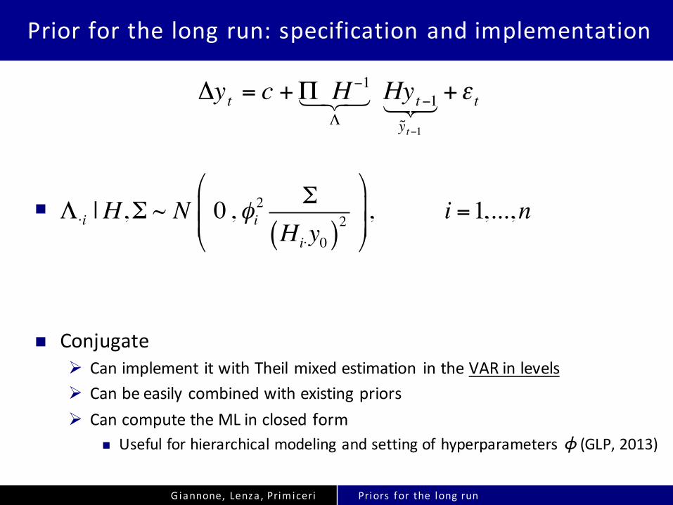
Priorforthelongrun:specificationandimplementation
n
€
Δyt = c +Π H −1
Λ! " # Hyt−1
˜ y t−1
! " # +ε t
Λ⋅i |H,Σ ~ N 0 , φi2 Σ
Hi⋅y0( )2 $
%&&
'
()), i =1,...,n
Page 32
Giannone,Lenza,Prim iceri Priors for the long run
Priorforthelongrun:specificationandimplementation
n
€
Δyt = c +Π H −1
Λ! " # Hyt−1
˜ y t−1
! " # +ε t
Λ⋅i |H,Σ ~ N 0 , φi2 Σ
Hi⋅y0( )2 $
%&&
'
()), i =1,...,n
Page 33
Giannone,Lenza,Prim iceri Priors for the long run
Priorforthelongrun:specificationandimplementation
n
n ConjugateØ Canimplement itwithTheilmixedestimation intheVARinlevels
€
Δyt = c +Π H −1
Λ! " # Hyt−1
˜ y t−1
! " # +ε t
Λ⋅i |H,Σ ~ N 0 , φi2 Σ
Hi⋅y0( )2 $
%&&
'
()), i =1,...,n
Page 34
Giannone,Lenza,Prim iceri Priors for the long run
Priorforthelongrun:specificationandimplementation
n
n ConjugateØ Canimplement itwithTheilmixedestimation intheVARinlevelsØ Canbeeasilycombinedwithexistingpriors
€
Δyt = c +Π H −1
Λ! " # Hyt−1
˜ y t−1
! " # +ε t
Λ⋅i |H,Σ ~ N 0 , φi2 Σ
Hi⋅y0( )2 $
%&&
'
()), i =1,...,n
Page 35
Giannone,Lenza,Prim iceri Priors for the long run
Priorforthelongrun:specificationandimplementation
n
n ConjugateØ Canimplement itwithTheilmixedestimation intheVARinlevelsØ CanbeeasilycombinedwithexistingpriorsØ CancomputetheMLinclosedform
n Usefulforhierarchicalmodelingandsettingofhyperparameters ϕ (GLP,2013)
€
Δyt = c +Π H −1
Λ! " # Hyt−1
˜ y t−1
! " # +ε t
Λ⋅i |H,Σ ~ N 0 , φi2 Σ
Hi⋅y0( )2 $
%&&
'
()), i =1,...,n
Page 36
Giannone,Lenza,Prim iceri Priors for the long run
Empiricalresults
n Deterministiccomponentin7-variableVAR
n ForecastingØ 3-variableVARØ 5-variableVARØ 7-variableVAR
Page 37
Giannone,Lenza,Prim iceri Priors for the long run
Empiricalresults
n Deterministiccomponentin7-variableVAR
Page 38
Giannone,Lenza,Prim iceri Priors for the long run
Empiricalresults
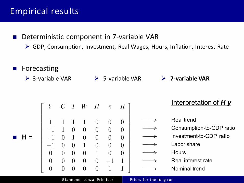
n Deterministiccomponentin7-variableVARØ GDP,Consumption,Investment,RealWages,Hours,Inflation,InterestRate
Page 39
Giannone,Lenza,Prim iceri Priors for the long run
Empiricalresults
n Deterministiccomponentin7-variableVARØ GDP,Consumption,Investment,RealWages,Hours,Inflation,InterestRate
n H=
Real trendConsumption-to-GDP ratioInvestment-to-GDP ratioLabor shareHoursReal interest rateNominal trend
Interpretation of H y2
6666666666664
Y C I W H ⇡ R
1 1 1 1 0 0 0�1 1 0 0 0 0 0�1 0 1 0 0 0 0�1 0 0 1 0 0 00 0 0 0 1 0 00 0 0 0 0 �1 10 0 0 0 0 1 1
3
7777777777775
1
Page 40
Giannone,Lenza,Prim iceri Priors for the long run
Empiricalresults
n Deterministiccomponentin7-variableVARØ GDP,Consumption,Investment,RealWages,Hours,Inflation,InterestRate
n ForecastingØ 3-variableVAR
n H=
Real trendConsumption-to-GDP ratioInvestment-to-GDP ratioLabor shareHoursReal interest rateNominal trend
Interpretation of H y2
6666666666664
Y C I W H ⇡ R
1 1 1 1 0 0 0�1 1 0 0 0 0 0�1 0 1 0 0 0 0�1 0 0 1 0 0 00 0 0 0 1 0 00 0 0 0 0 �1 10 0 0 0 0 1 1
3
7777777777775
1
Ø 5-variableVAR Ø 7-variableVAR
Page 41
Giannone,Lenza,Prim iceri Priors for the long run
Empiricalresults
n Deterministiccomponentin7-variableVARØ GDP,Consumption,Investment,RealWages,Hours,Inflation,InterestRate
n ForecastingØ 3-variableVAR
n H=
Real trendConsumption-to-GDP ratioInvestment-to-GDP ratioLabor shareHoursReal interest rateNominal trend
Interpretation of H y2
6666666666664
Y C I W H ⇡ R
1 1 1 1 0 0 0�1 1 0 0 0 0 0�1 0 1 0 0 0 0�1 0 0 1 0 0 00 0 0 0 1 0 00 0 0 0 0 �1 10 0 0 0 0 1 1
3
7777777777775
1
Ø 5-variableVAR Ø 7-variableVAR
Page 42
Giannone,Lenza,Prim iceri Priors for the long run
Empiricalresults
n Deterministiccomponentin7-variableVARØ GDP,Consumption,Investment,RealWages,Hours,Inflation,InterestRate
n ForecastingØ 3-variableVAR
n H=
Real trendConsumption-to-GDP ratioInvestment-to-GDP ratioLabor shareHoursReal interest rateNominal trend
Interpretation of H y2
6666666666664
Y C I W H ⇡ R
1 1 1 1 0 0 0�1 1 0 0 0 0 0�1 0 1 0 0 0 0�1 0 0 1 0 0 00 0 0 0 1 0 00 0 0 0 0 �1 10 0 0 0 0 1 1
3
7777777777775
1
Ø 5-variableVAR Ø 7-variableVAR
Page 43
Giannone,Lenza,Prim iceri Priors for the long run
DeterministiccomponentsinVARs
1960 1980 2000
5.55.65.75.85.9
66.16.26.36.4
GDP
1960 1980 20003.9
44.14.24.34.44.54.64.7
Investment
1960 1980 2000
-0.65
-0.6
-0.55
-0.5
Hours
1960 1980 2000
-1.7-1.65
-1.6-1.55
-1.5-1.45
-1.4-1.35
-1.3-1.25
Investment-to-GDP ratio
1960 1980 2000-0.015
-0.01-0.005
00.005
0.010.015
0.020.025
Inflation
1960 1980 2000
-0.01
0
0.01
0.02
0.03
0.04
Interest rate
Data Flat MN PLR
Page 44
Giannone,Lenza,Prim iceri Priors for the long run
DeterministiccomponentsinVARswithPriorfortheLongRun
1960 1980 2000
5.5
6
6.5GDP
1960 1980 2000
4
4.2
4.4
4.6
4.8
5Investment
1960 1980 2000
-0.65
-0.6
-0.55
-0.5
Hours
1960 1980 2000
-1.7-1.65
-1.6-1.55
-1.5-1.45
-1.4-1.35
-1.3-1.25
Investment-to-GDP ratio
1960 1980 2000-0.015
-0.01-0.005
00.005
0.010.015
0.020.025
Inflation
1960 1980 2000
-0.01
0
0.01
0.02
0.03
0.04
Interest rate
Data Flat MN PLR
Page 45
Giannone,Lenza,Prim iceri Priors for the long run
Forecastingresultswith3-,5- and7-variableVARs
n Recursiveestimationstartsin1955:I
n Forecast-evaluationsample:1985:I– 2013:I
Page 46
Giannone,Lenza,Prim iceri Priors for the long run
3-variableVAR:MSFE(1985-2013)
0 10 20 30 40
MSF
E
0
0.002
0.004
0.006
0.008
0.01Y
Quarters ahead0 10 20 30 40
MSF
E
0
0.02
0.04
0.06
0.08
0.1
0.12
0.14Y + C + I
0 10 20 30 40 0
0.002
0.004
0.006
0.008
0.01
0.012
0.014C
Quarters ahead0 10 20 30 40
0
0.0002
0.0004
0.0006
0.0008
0.001
0.0012C - Y
0 10 20 30 40 0
0.01
0.02
0.03
0.04
0.05
0
0.01
0.02
0.03I
Quarters ahead0 10 20 30 40
0
0.005
0.01
0.015
0.02
0.025
0.03I - Y
MN SZ Naive PLR
Page 47
Giannone,Lenza,Prim iceri Priors for the long run
3-variableVAR:MSFE(1985-2013)
0 10 20 30 40
MSF
E
0
0.002
0.004
0.006
0.008
0.01Y
Quarters ahead0 10 20 30 40
MSF
E
0
0.02
0.04
0.06
0.08
0.1
0.12
0.14Y + C + I
0 10 20 30 40 0
0.002
0.004
0.006
0.008
0.01
0.012
0.014C
Quarters ahead0 10 20 30 40
0
0.0002
0.0004
0.0006
0.0008
0.001
0.0012C - Y
0 10 20 30 40 0
0.01
0.02
0.03
0.04
0.05I
Quarters ahead0 10 20 30 40
0
0.005
0.01
0.015
0.02
0.025
0.03I - Y
MN SZ Naive PLR
Page 48
Giannone,Lenza,Prim iceri Priors for the long run
Consumption- andInvestment-to-GDPratios
1960 1970 1980 1990 2000 2010-0.65
-0.6
-0.55
-0.5
C - Y
1960 1970 1980 1990 2000 2010-1.7
-1.6
-1.5
-1.4
-1.3
I - Y
Actual Naive PLR
Page 49
Giannone,Lenza,Prim iceri Priors for the long run
Forecasts(5yearsahead)
1960 1970 1980 1990 2000 2010-0.65
-0.6
-0.55
-0.5
C - Y
1960 1970 1980 1990 2000 2010-1.7
-1.6
-1.5
-1.4
-1.3
I - Y
Actual Naive PLR
Page 50
Giannone,Lenza,Prim iceri Priors for the long run
Forecasts(5yearsahead)
1960 1970 1980 1990 2000 2010-0.65
-0.6
-0.55
-0.5
C - Y
1960 1970 1980 1990 2000 2010-1.7
-1.6
-1.5
-1.4
-1.3
I - Y
Actual Naive PLR
Page 51
Giannone,Lenza,Prim iceri Priors for the long run
5-variableVAR:MSFE(1985-2013)
0 10 20 30 40
MSF
E
0
0.001
0.002
0.003
0.004
0.005
0.006
0.007
0.008Y
0 10 20 30 40M
SFE
0
0.002
0.004
0.006
0.008
0.01
0.012C
0 10 20 30 40
MSF
E
0
0.01
0.02
0.03
0.04
0.05
0.06
0.07
0.08I
Quarters Ahead0 10 20 30 40
MSF
E
0
0.001
0.002
0.003
0.004
0.005
0.006
0.007H
Quarters Ahead0 10 20 30 40
MSF
E
0
0.002
0.004
0.006
0.008
0.01
0.012W
MNSZNaivePLR
Page 52
Giannone,Lenza,Prim iceri Priors for the long run
7-variableVAR:MSFE(1985-2013)
0 20 40
MSF
E
00.0010.0020.0030.0040.0050.0060.0070.0080.009 0.01
Y
0 20 40
MSF
E
0
0.002
0.004
0.006
0.008
0.01
0.012
0.014C
0 20 40
MSF
E
0
0.01
0.02
0.03
0.04
0.05
0.06
0.07
0.08I
0 20 40
MSF
E
0
0.001
0.002
0.003
0.004
0.005
0.006
0.007
0.008
0.009H
Quarters Ahead0 20 40
MSF
E
00.0020.0040.0060.008 0.01
0.0120.0140.0160.018 0.02
W
Quarters Ahead0 20 40
MSF
E
0
2e-05
4e-05
6e-05
8e-05
0.0001
0.00012:
Quarters Ahead0 20 40
MSF
E
0
5e-05
0.0001
0.00015
0.0002
0.00025
0.0003R
MNSZNaivePLR
𝝅
Page 53
Giannone,Lenza,Prim iceri Priors for the long run
Invariancetorotationsofthe“stationary”space
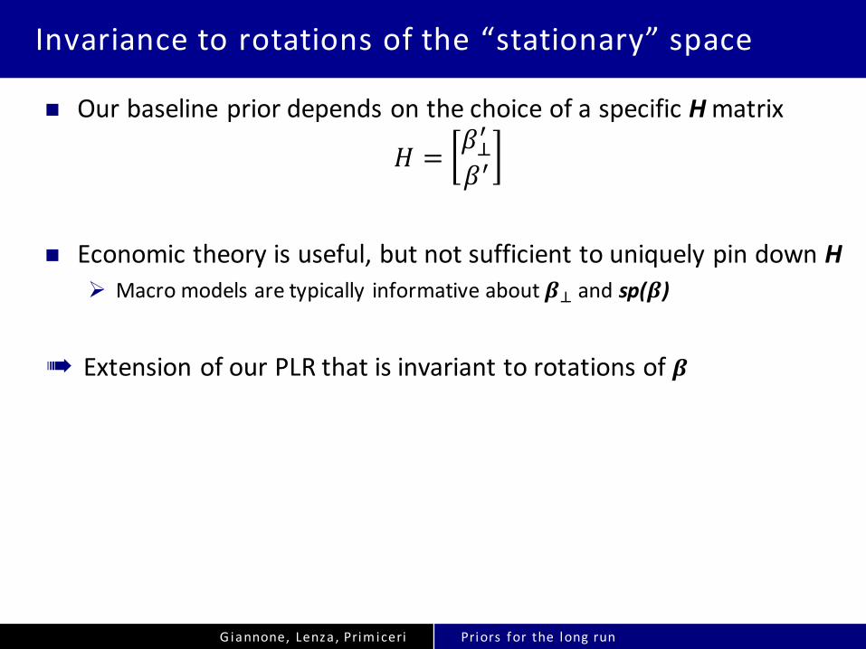
n OurbaselinepriordependsonthechoiceofaspecificHmatrix
𝐻 = 𝛽%&
𝛽&
Page 54
Giannone,Lenza,Prim iceri Priors for the long run
Invariancetorotationsofthe“stationary”space
n OurbaselinepriordependsonthechoiceofaspecificHmatrix
𝐻 = 𝛽%&
𝛽&
n Economictheoryisuseful,butnotsufficienttouniquelypindownHØ Macromodelsaretypically informativeabout𝜷%andsp(𝜷)
Page 55
Giannone,Lenza,Prim iceri Priors for the long run
Invariancetorotationsofthe“stationary”space
n OurbaselinepriordependsonthechoiceofaspecificHmatrix
𝐻 = 𝛽%&
𝛽&
n Economictheoryisuseful,butnotsufficienttouniquelypindownHØ Macromodelsaretypically informativeabout𝜷%andsp(𝜷)
➠ ExtensionofourPLRthatisinvarianttorotationsof𝜷
Page 56
Giannone,Lenza,Prim iceri Priors for the long run
Invariancetorotationsofthe“stationary”space
n OurbaselinepriordependsonthechoiceofaspecificHmatrix
𝐻 = 𝛽%&
𝛽&
n Economictheoryisuseful,butnotsufficienttouniquelypindownHØ Macromodelsaretypically informativeabout𝜷%andsp(𝜷)
➠ ExtensionofourPLRthatisinvarianttorotationsof𝜷
BaselinePLR: Λ*+ * 𝐻+*𝑦-. |𝐻, Σ~𝑁 0,𝜙+6Σ , 𝑖 = 1, … ,𝑛
Page 57
Giannone,Lenza,Prim iceri Priors for the long run
Invariancetorotationsofthe“stationary”space
n OurbaselinepriordependsonthechoiceofaspecificHmatrix
𝐻 = 𝛽%&
𝛽&
n Economictheoryisuseful,butnotsufficienttouniquelypindownHØ Macromodelsaretypically informativeabout𝜷%andsp(𝜷)
➠ ExtensionofourPLRthatisinvarianttorotationsof𝜷
BaselinePLR: Λ*+ * 𝐻+*𝑦-. |𝐻, Σ~𝑁 0,𝜙+6Σ , 𝑖 = 1, … ,𝑛
InvariantPLR: ;Λ*+ * 𝐻+*𝑦-. |𝐻, Σ~𝑁 0,𝜙+6Σ , 𝑖 = 1, … ,𝑛 − 𝑟
∑ Λ*+ * 𝐻+*𝑦-. |𝐻, Σ~𝑁 0,𝜙?@ABC6 Σ?+D?@ABC
Page 58
Giannone,Lenza,Prim iceri Priors for the long run
7-variableVAR:Forecasting resultswith“invariant”PLR
0 20 40
MS
FE
0
0.002
0.004
0.006
0.008
0.01Y
0 20 40M
SFE
0
0.002
0.004
0.006
0.008
0.01C
0 20 40
MS
FE
0
0.01
0.02
0.03
0.04
0.05I
0 20 40
MS
FE
0
0.002
0.004
0.006
0.008H
0 20 40
MS
FE
0
2e-05
4e-05
6e-05
8e-05
0.0001π
0 20 40M
SFE
0
2e-05
4e-05
6e-05
8e-05
0.0001
0.00012R
Quarters Ahead0 20 40
MS
FE
0
0.0005
0.001
0.0015
0.002
0.0025
0.003C - Y
Quarters Ahead0 20 40
MS
FE
0
0.005
0.01
0.015
0.02
0.025I - Y
Quarters Ahead0 20 40
MS
FE
0
0.0005
0.001
0.0015
0.002W - Y
PLR baseline PLR invariant PLR invariant (except C-Y)
Page 59
Giannone,Lenza,Prim iceri Priors for the long run
Hy inthedata
1940 1960 1980 2000 2020-0.7
-0.65
-0.6
-0.55
-0.5
-0.45C-Y
1940 1960 1980 2000 2020-1.8
-1.7
-1.6
-1.5
-1.4
-1.3
-1.2I-Y
1940 1960 1980 2000 2020-0.72-0.7-0.68-0.66-0.64-0.62-0.6-0.58-0.56-0.54-0.52
H
1940 1960 1980 2000 2020-0.62
-0.6
-0.58
-0.56
-0.54
-0.52
-0.5W-Y
1940 1960 1980 2000 2020-0.01
0
0.01
0.02
0.03
0.04
0.05
0.06
0.07R+:
1940 1960 1980 2000 2020-0.01
-0.005
0
0.005
0.01
0.015
0.02
0.025
0.03R-:𝝅 𝝅
Page 60
Giannone,Lenza,Prim iceri Priors for the long run
7-variableVAR:Forecasting resultswith“invariant”PLR
0 20 40
MS
FE
0
0.002
0.004
0.006
0.008
0.01Y
0 20 40M
SFE
0
0.002
0.004
0.006
0.008
0.01C
0 20 40
MS
FE
0
0.01
0.02
0.03
0.04
0.05I
0 20 40
MS
FE
0
0.002
0.004
0.006
0.008H
0 20 40
MS
FE
0
2e-05
4e-05
6e-05
8e-05
0.0001π
0 20 40M
SFE
0
2e-05
4e-05
6e-05
8e-05
0.0001
0.00012R
Quarters Ahead0 20 40
MS
FE
0
0.0005
0.001
0.0015
0.002
0.0025
0.003C - Y
Quarters Ahead0 20 40
MS
FE
0
0.005
0.01
0.015
0.02
0.025I - Y
Quarters Ahead0 20 40
MS
FE
0
0.0005
0.001
0.0015
0.002W - Y
PLR baseline PLR invariant PLR invariant (except C-Y)
Page 61
Giannone,Lenza,Prim iceri Priors for the long run
Strengthsandweaknesses
n StrengthsØ Imposesdiscipline onlong-runbehaviorofthemodelØ BasedonrobustlessonsoftheoreticalmacromodelsØ Performswellinforecasting(especially atlongerhorizons)Ø Veryeasytoimplement
Page 62
Giannone,Lenza,Prim iceri Priors for the long run
Strengthsandweaknesses
n StrengthsØ Imposesdiscipline onlong-runbehaviorofthemodelØ BasedonrobustlessonsoftheoreticalmacromodelsØ Performswellinforecasting(especially atlongerhorizons)Ø Veryeasytoimplement
n “Weak”pointsØ Non-automaticprocedureà needtothinkaboutitØ Mightprovedifficulttosetupinlarge-scalemodelsà mightrequiretoo
muchthinking
Page 63
Giannone,Lenza,Prim iceri Priors for the long run
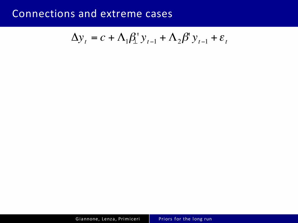
Connectionsandextremecases
n Rewriteas
€
Δyt = c +Π H −1
Λ! " # Hyt−1
˜ y t−1
! " # +ε t
Δyt = c+ Λ1 Λ2[ ] β⊥ 'β '$
%&
'
()yt−1 +εt
Page 64
Giannone,Lenza,Prim iceri Priors for the long run
Connectionsandextremecases
n Rewriteas
€
Δyt = c +Π H −1
Λ! " # Hyt−1
˜ y t−1
! " # +ε t
Δyt = c+ Λ1 Λ2[ ] β⊥ 'β '$
%&
'
()yt−1 +εt
Δyt = c+Λ1β⊥ ' yt−1 +Λ2β ' yt−1 +εt
Page 65
Giannone,Lenza,Prim iceri Priors for the long run
Connectionsandextremecases
€
Δyt = c +Λ1β⊥' yt−1 +Λ2β' yt−1 +ε t
Page 66
Giannone,Lenza,Prim iceri Priors for the long run
Connectionsandextremecases
n ErrorCorrectionModel:dogmaticprioronΛ1=0
€
Δyt = c +Λ1β⊥' yt−1 +Λ2β' yt−1 +ε t
Page 67
Giannone,Lenza,Prim iceri Priors for the long run
Connectionsandextremecases
n ErrorCorrectionModel:dogmaticprioronΛ1=0
€
Δyt = c +Λ1β⊥' yt−1 +Λ2β' yt−1 +ε t
Ø KPSW,CEEn fixβ basedontheoryn flatprioronΛ2
Page 68
Giannone,Lenza,Prim iceri Priors for the long run
Connectionsandextremecases
n ErrorCorrectionModel:dogmaticprioronΛ1=0
€
Δyt = c +Λ1β⊥' yt−1 +Λ2β' yt−1 +ε t
Ø KPSW,CEEn fixβ basedontheoryn flatprioronΛ2
Ø Cointegrationn estimateβn flatprioronΛ2
n EG(1987)
Page 69
Giannone,Lenza,Prim iceri Priors for the long run
Connectionsandextremecases
n ErrorCorrectionModel:dogmaticprioronΛ1=0
€
Δyt = c +Λ1β⊥' yt−1 +Λ2β' yt−1 +ε t
Ø Bayesiancointegrationn uniform prioronsp(β)n KSvDV (2006)
Ø Cointegrationn estimateβn flatprioronΛ2
n EG(1987)
Ø KPSW,CEEn fixβ basedontheoryn flatprioronΛ2
Page 70
Giannone,Lenza,Prim iceri Priors for the long run
Connectionsandextremecases
n ErrorCorrectionModel:dogmaticprioronΛ1=0
n VARinfirstdifferences:dogmaticprioronΛ1=Λ2=0
€
Δyt = c +Λ1β⊥' yt−1 +Λ2β' yt−1 +ε t
Ø KPSW,CEEn fixβ basedontheoryn flatprioronΛ2
Ø Cointegrationn estimateβn flatprioronΛ2
n EG(1987)
Ø Bayesiancointegrationn uniform prioronsp(β)n KSvDV (2006)
Page 71
Giannone,Lenza,Prim iceri Priors for the long run
Connectionsandextremecases
n ErrorCorrectionModel:dogmaticprioronΛ1=0
n VARinfirstdifferences:dogmaticprioronΛ1=Λ2=0
n Sum-of-coefficientsprior(DLS,SZ)Ø [β’ β’]’ =H=IØ shrinkΛ1 andΛ2 to0
€
Δyt = c +Λ1β⊥' yt−1 +Λ2β' yt−1 +ε t
Ø KPSW,CEEn fixβ basedontheoryn flatprioronΛ2
Ø Cointegrationn estimateβn flatprioronΛ2
n EG(1987)
Ø Bayesiancointegrationn uniform prioronsp(β)n KSvDV (2006)
Page 72
Giannone,Lenza,Prim iceri Priors for the long run
3-varVAR:MeanSquaredForecastErrors(1985-2013)
0 10 20 30 40
MSF
E
0
0.002
0.004
0.006
0.008
0.01Y
Quarters ahead0 10 20 30 40
MSF
E
0
0.02
0.04
0.06
0.08
0.1
0.12
0.14Y + C + I
0 10 20 30 40 0
0.002
0.004
0.006
0.008
0.01
0.012
0.014C
Quarters ahead0 10 20 30 40
0
0.0002
0.0004
0.0006
0.0008
0.001
0.0012C - Y
0 10 20 30 40 0
0.01
0.02
0.03
0.04
0.05I
Quarters ahead0 10 20 30 40
0
0.005
0.01
0.015
0.02
0.025
0.03I - Y
MN SZ Naive PLR