384
Notes on Theory of Distributed Systems CS 465/565: Spring 2014 James Aspnes 2014-05-02 18:02
| Date post: | 25-Dec-2015 |
| Category: |
Documents |
| Upload: | abir-dutta |
| View: | 3 times |
| Download: | 0 times |

Notes on Theory of Distributed SystemsCS 465/565: Spring 2014
James Aspnes
2014-05-02 18:02

Contents
Table of contents i
List of figures xi
List of tables xii
List of algorithms xiii
Preface xvii
Syllabus xviii
Lecture schedule xxi
1 Introduction 1
I Message passing 5
2 Model 62.1 Basic message-passing model . . . . . . . . . . . . . . . . . . 6
2.1.1 Formal details . . . . . . . . . . . . . . . . . . . . . . 62.1.2 Network structure . . . . . . . . . . . . . . . . . . . . 8
2.2 Asynchronous systems . . . . . . . . . . . . . . . . . . . . . . 82.2.1 Example: client-server computing . . . . . . . . . . . . 8
2.3 Synchronous systems . . . . . . . . . . . . . . . . . . . . . . . 102.4 Complexity measures . . . . . . . . . . . . . . . . . . . . . . . 10
3 Coordinated attack 123.1 Formal description . . . . . . . . . . . . . . . . . . . . . . . . 123.2 Impossibility proof . . . . . . . . . . . . . . . . . . . . . . . . 13
i

CONTENTS ii
3.3 Randomized coordinated attack . . . . . . . . . . . . . . . . . 143.3.1 An algorithm . . . . . . . . . . . . . . . . . . . . . . . 153.3.2 Why it works . . . . . . . . . . . . . . . . . . . . . . . 163.3.3 Almost-matching lower bound . . . . . . . . . . . . . . 17
4 Broadcast and convergecast 184.1 Flooding . . . . . . . . . . . . . . . . . . . . . . . . . . . . . . 18
4.1.1 Basic algorithm . . . . . . . . . . . . . . . . . . . . . . 184.1.2 Adding parent pointers . . . . . . . . . . . . . . . . . 204.1.3 Termination . . . . . . . . . . . . . . . . . . . . . . . . 21
4.2 Convergecast . . . . . . . . . . . . . . . . . . . . . . . . . . . 224.3 Flooding and convergecast together . . . . . . . . . . . . . . . 23
5 Distributed breadth-first search 255.1 Using explicit distances . . . . . . . . . . . . . . . . . . . . . 255.2 Using layering . . . . . . . . . . . . . . . . . . . . . . . . . . . 275.3 Using local synchronization . . . . . . . . . . . . . . . . . . . 27
6 Leader election 316.1 Symmetry . . . . . . . . . . . . . . . . . . . . . . . . . . . . . 326.2 Leader election in rings . . . . . . . . . . . . . . . . . . . . . 33
6.2.1 The Le-Lann-Chang-Roberts algorithm . . . . . . . . 336.2.1.1 Proof of correctness for synchronous executions 346.2.1.2 Performance . . . . . . . . . . . . . . . . . . 34
6.2.2 The Hirschberg-Sinclair algorithm . . . . . . . . . . . 356.2.3 Peterson’s algorithm for the unidirectional ring . . . . 356.2.4 A simple randomized O(n logn)-message algorithm . . 36
6.3 Leader election in general networks . . . . . . . . . . . . . . . 386.4 Lower bounds . . . . . . . . . . . . . . . . . . . . . . . . . . . 38
6.4.1 Lower bound on asynchronous message complexity . . 396.4.2 Lower bound for comparison-based algorithms . . . . 40
7 Synchronous agreement 437.1 Problem definition . . . . . . . . . . . . . . . . . . . . . . . . 437.2 Lower bound on rounds . . . . . . . . . . . . . . . . . . . . . 447.3 Solutions . . . . . . . . . . . . . . . . . . . . . . . . . . . . . 46
7.3.1 Flooding . . . . . . . . . . . . . . . . . . . . . . . . . . 467.4 Exponential information gathering . . . . . . . . . . . . . . . 47
7.4.1 Basic invariants . . . . . . . . . . . . . . . . . . . . . . 487.4.2 Stronger facts . . . . . . . . . . . . . . . . . . . . . . . 49

CONTENTS iii
7.4.3 The payoff . . . . . . . . . . . . . . . . . . . . . . . . 497.4.4 The real payoff . . . . . . . . . . . . . . . . . . . . . . 49
7.5 Variants . . . . . . . . . . . . . . . . . . . . . . . . . . . . . . 49
8 Byzantine agreement 508.1 Lower bounds . . . . . . . . . . . . . . . . . . . . . . . . . . . 50
8.1.1 Minimum number of rounds . . . . . . . . . . . . . . . 508.1.2 Minimum number of processes . . . . . . . . . . . . . 508.1.3 Minimum connectivity . . . . . . . . . . . . . . . . . . 528.1.4 Weak Byzantine agreement . . . . . . . . . . . . . . . 53
8.2 Upper bounds . . . . . . . . . . . . . . . . . . . . . . . . . . . 548.2.1 Exponential information gathering gets n = 3f + 1 . . 55
8.2.1.1 Proof of correctness . . . . . . . . . . . . . . 558.2.2 Phase king gets constant-size messages . . . . . . . . . 57
8.2.2.1 The algorithm . . . . . . . . . . . . . . . . . 578.2.2.2 Proof of correctness . . . . . . . . . . . . . . 598.2.2.3 Performance of phase king . . . . . . . . . . 59
9 Impossibility of asynchronous agreement 619.1 Agreement . . . . . . . . . . . . . . . . . . . . . . . . . . . . . 629.2 Failures . . . . . . . . . . . . . . . . . . . . . . . . . . . . . . 629.3 Steps . . . . . . . . . . . . . . . . . . . . . . . . . . . . . . . . 629.4 Bivalence and univalence . . . . . . . . . . . . . . . . . . . . . 639.5 Existence of an initial bivalent configuration . . . . . . . . . . 639.6 Staying in a bivalent configuration . . . . . . . . . . . . . . . 649.7 Generalization to other models . . . . . . . . . . . . . . . . . 65
10 Paxos 6610.1 Motivation: replicated state machines . . . . . . . . . . . . . 6610.2 The Paxos algorithm . . . . . . . . . . . . . . . . . . . . . . . 6710.3 Informal analysis: how information flows between rounds . . 6910.4 Safety properties . . . . . . . . . . . . . . . . . . . . . . . . . 6910.5 Learning the results . . . . . . . . . . . . . . . . . . . . . . . 7110.6 Liveness properties . . . . . . . . . . . . . . . . . . . . . . . . 71
11 Failure detectors 7311.1 How to build a failure detector . . . . . . . . . . . . . . . . . 7411.2 Classification of failure detectors . . . . . . . . . . . . . . . . 74
11.2.1 Degrees of completeness . . . . . . . . . . . . . . . . . 7411.2.2 Degrees of accuracy . . . . . . . . . . . . . . . . . . . 74

CONTENTS iv
11.2.3 Boosting completeness . . . . . . . . . . . . . . . . . . 7511.2.4 Failure detector classes . . . . . . . . . . . . . . . . . . 76
11.3 Consensus with S . . . . . . . . . . . . . . . . . . . . . . . . . 7711.3.1 Proof of correctness . . . . . . . . . . . . . . . . . . . 78
11.4 Consensus with ♦S and f < n/2 . . . . . . . . . . . . . . . . 7911.4.1 Proof of correctness . . . . . . . . . . . . . . . . . . . 81
11.5 f < n/2 is still required even with ♦P . . . . . . . . . . . . . 8211.6 Relationships among the classes . . . . . . . . . . . . . . . . . 83
12 Logical clocks 8512.1 Causal ordering . . . . . . . . . . . . . . . . . . . . . . . . . . 8512.2 Implementations . . . . . . . . . . . . . . . . . . . . . . . . . 87
12.2.1 Lamport clock . . . . . . . . . . . . . . . . . . . . . . 8712.2.2 Neiger-Toueg-Welch clock . . . . . . . . . . . . . . . . 8812.2.3 Vector clocks . . . . . . . . . . . . . . . . . . . . . . . 89
12.3 Applications . . . . . . . . . . . . . . . . . . . . . . . . . . . . 8912.3.1 Consistent snapshots . . . . . . . . . . . . . . . . . . . 89
12.3.1.1 Property testing . . . . . . . . . . . . . . . . 9112.3.2 Replicated state machines . . . . . . . . . . . . . . . . 91
13 Synchronizers 9313.1 Definitions . . . . . . . . . . . . . . . . . . . . . . . . . . . . . 9313.2 Implementations . . . . . . . . . . . . . . . . . . . . . . . . . 94
13.2.1 The alpha synchronizer . . . . . . . . . . . . . . . . . 9513.2.2 The beta synchronizer . . . . . . . . . . . . . . . . . . 9513.2.3 The gamma synchronizer . . . . . . . . . . . . . . . . 96
13.3 Applications . . . . . . . . . . . . . . . . . . . . . . . . . . . . 9713.4 Limitations of synchronizers . . . . . . . . . . . . . . . . . . . 97
13.4.1 Impossibility with crash failures . . . . . . . . . . . . 9713.4.2 Unavoidable slowdown with global synchronization . . 97
13.5 Outline of the proof . . . . . . . . . . . . . . . . . . . . . . . 98
14 Quorum systems 10014.1 Basics . . . . . . . . . . . . . . . . . . . . . . . . . . . . . . . 10014.2 Simple quorum systems . . . . . . . . . . . . . . . . . . . . . 10014.3 Goals . . . . . . . . . . . . . . . . . . . . . . . . . . . . . . . 10114.4 Paths system . . . . . . . . . . . . . . . . . . . . . . . . . . . 10214.5 Byzantine quorum systems . . . . . . . . . . . . . . . . . . . 10314.6 Probabilistic quorum systems . . . . . . . . . . . . . . . . . . 104
14.6.1 Example . . . . . . . . . . . . . . . . . . . . . . . . . . 105

CONTENTS v
14.6.2 Performance . . . . . . . . . . . . . . . . . . . . . . . 10514.7 Signed quorum systems . . . . . . . . . . . . . . . . . . . . . 106
II Shared memory 107
15 Model 10815.1 Atomic registers . . . . . . . . . . . . . . . . . . . . . . . . . 10815.2 Single-writer versus multi-writer registers . . . . . . . . . . . 10915.3 Fairness and crashes . . . . . . . . . . . . . . . . . . . . . . . 11015.4 Concurrent executions . . . . . . . . . . . . . . . . . . . . . . 11015.5 Consistency properties . . . . . . . . . . . . . . . . . . . . . . 11115.6 Complexity measures . . . . . . . . . . . . . . . . . . . . . . . 11215.7 Fancier registers . . . . . . . . . . . . . . . . . . . . . . . . . 113
16 Distributed shared memory 11516.1 Message passing from shared memory . . . . . . . . . . . . . 11616.2 The Attiya-Bar-Noy-Dolev algorithm . . . . . . . . . . . . . . 11616.3 Proof of linearizability . . . . . . . . . . . . . . . . . . . . . . 11816.4 Proof that f < n/2 is necessary . . . . . . . . . . . . . . . . . 11916.5 Multiple writers . . . . . . . . . . . . . . . . . . . . . . . . . . 11916.6 Other operations . . . . . . . . . . . . . . . . . . . . . . . . . 120
17 Mutual exclusion 12117.1 The problem . . . . . . . . . . . . . . . . . . . . . . . . . . . 12117.2 Goals . . . . . . . . . . . . . . . . . . . . . . . . . . . . . . . 12117.3 Mutual exclusion using strong primitives . . . . . . . . . . . . 122
17.3.1 Test and set . . . . . . . . . . . . . . . . . . . . . . . . 12217.3.2 A lockout-free algorithm using an atomic queue . . . . 123
17.3.2.1 Reducing space complexity . . . . . . . . . . 12417.4 Mutual exclusion using only atomic registers . . . . . . . . . 125
17.4.1 Peterson’s tournament algorithm . . . . . . . . . . . . 12517.4.1.1 Correctness of Peterson’s protocol . . . . . . 12617.4.1.2 Generalization to n processes . . . . . . . . . 129
17.4.2 Fast mutual exclusion . . . . . . . . . . . . . . . . . . 12917.4.3 Lamport’s Bakery algorithm . . . . . . . . . . . . . . 13217.4.4 Lower bound on the number of registers . . . . . . . . 133
17.5 RMR complexity . . . . . . . . . . . . . . . . . . . . . . . . . 13517.5.1 Cache-coherence vs. distributed shared memory . . . . 13517.5.2 RMR complexity of Peterson’s algorithm . . . . . . . 136

CONTENTS vi
17.5.3 Mutual exclusion in the DSM model . . . . . . . . . . 13717.5.4 Lower bounds . . . . . . . . . . . . . . . . . . . . . . . 139
18 The wait-free hierarchy 14018.1 Classification by consensus number . . . . . . . . . . . . . . . 141
18.1.1 Level 1: registers etc. . . . . . . . . . . . . . . . . . . 14218.1.2 Level 2: interfering RMW objects etc. . . . . . . . . . 14318.1.3 Level ∞: objects where first write wins . . . . . . . . 14518.1.4 Level 2m− 2: simultaneous m-register write . . . . . . 146
18.1.4.1 Matching impossibility result . . . . . . . . . 14818.1.5 Level m: m-process consensus objects . . . . . . . . . 149
18.2 Universality of consensus . . . . . . . . . . . . . . . . . . . . . 150
19 Atomic snapshots 15319.1 The basic trick: two identical collects equals a snapshot . . . 15319.2 The Gang of Six algorithm . . . . . . . . . . . . . . . . . . . 154
19.2.1 Linearizability . . . . . . . . . . . . . . . . . . . . . . 15519.2.2 Using bounded registers . . . . . . . . . . . . . . . . . 156
19.3 Faster snapshots using lattice agreement . . . . . . . . . . . . 15919.3.1 Lattice agreement . . . . . . . . . . . . . . . . . . . . 15919.3.2 Connection to vector clocks . . . . . . . . . . . . . . . 16019.3.3 The full reduction . . . . . . . . . . . . . . . . . . . . 16019.3.4 Why this works . . . . . . . . . . . . . . . . . . . . . . 16219.3.5 Implementing lattice agreement . . . . . . . . . . . . . 163
19.4 Practical snapshots using LL/SC . . . . . . . . . . . . . . . . 16719.4.1 Details of the single-scanner snapshot . . . . . . . . . 16819.4.2 Extension to multiple scanners . . . . . . . . . . . . . 170
19.5 Applications . . . . . . . . . . . . . . . . . . . . . . . . . . . . 17019.5.1 Multi-writer registers from single-writer registers . . . 17019.5.2 Counters and accumulators . . . . . . . . . . . . . . . 17119.5.3 Resilient snapshot objects . . . . . . . . . . . . . . . . 171
20 Lower bounds on perturbable objects 173
21 Restricted-use objects 17621.1 Implementing bounded max registers . . . . . . . . . . . . . . 17621.2 Encoding the set of values . . . . . . . . . . . . . . . . . . . . 17821.3 Unbounded max registers . . . . . . . . . . . . . . . . . . . . 17921.4 Lower bound . . . . . . . . . . . . . . . . . . . . . . . . . . . 17921.5 Max-register snapshots . . . . . . . . . . . . . . . . . . . . . . 180

CONTENTS vii
21.5.1 Linearizability . . . . . . . . . . . . . . . . . . . . . . 18321.5.2 Application to standard snapshots . . . . . . . . . . . 183
22 Common2 18622.1 Test-and-set and swap for two processes . . . . . . . . . . . . 18722.2 Building n-process TAS from 2-process TAS . . . . . . . . . . 18722.3 Single-use swap objects . . . . . . . . . . . . . . . . . . . . . 189
23 Randomized consensus and test-and-set 19223.1 Role of the adversary in randomized algorithms . . . . . . . . 19223.2 History . . . . . . . . . . . . . . . . . . . . . . . . . . . . . . 19423.3 Reduction to simpler primitives . . . . . . . . . . . . . . . . . 194
23.3.1 Adopt-commit objects . . . . . . . . . . . . . . . . . . 19523.3.2 Conciliators . . . . . . . . . . . . . . . . . . . . . . . . 196
23.4 Implementing an adopt-commit object . . . . . . . . . . . . . 19623.5 A one-register conciliator for an oblivious adversary . . . . . 19723.6 Sifters . . . . . . . . . . . . . . . . . . . . . . . . . . . . . . . 199
23.6.1 Test-and-set using sifters . . . . . . . . . . . . . . . . 20123.6.2 Consensus using sifters . . . . . . . . . . . . . . . . . . 201
23.7 O(log∗ n) Randomized test-and-set . . . . . . . . . . . . . . . 20323.8 Space bounds . . . . . . . . . . . . . . . . . . . . . . . . . . . 205
24 Renaming 20724.1 Renaming . . . . . . . . . . . . . . . . . . . . . . . . . . . . . 20724.2 Performance . . . . . . . . . . . . . . . . . . . . . . . . . . . . 20824.3 Order-preserving renaming . . . . . . . . . . . . . . . . . . . 20924.4 Deterministic renaming . . . . . . . . . . . . . . . . . . . . . 209
24.4.1 Wait-free renaming with 2n− 1 names . . . . . . . . . 21024.4.2 Long-lived renaming . . . . . . . . . . . . . . . . . . . 21124.4.3 Renaming without snapshots . . . . . . . . . . . . . . 212
24.4.3.1 Splitters . . . . . . . . . . . . . . . . . . . . . 21224.4.3.2 Splitters in a grid . . . . . . . . . . . . . . . 213
24.4.4 Getting to 2n− 1 names in polynomial space . . . . . 21524.4.5 Renaming with test-and-set . . . . . . . . . . . . . . . 216
24.5 Randomized renaming . . . . . . . . . . . . . . . . . . . . . . 21624.5.1 Randomized splitters . . . . . . . . . . . . . . . . . . . 21724.5.2 Randomized test-and-set plus sampling . . . . . . . . 21724.5.3 Renaming with sorting networks . . . . . . . . . . . . 218
24.5.3.1 Sorting networks . . . . . . . . . . . . . . . . 21824.5.3.2 Renaming networks . . . . . . . . . . . . . . 219

CONTENTS viii
24.5.4 Randomized loose renaming . . . . . . . . . . . . . . . 220
25 Software transactional memory 22225.1 Motivation . . . . . . . . . . . . . . . . . . . . . . . . . . . . 22325.2 Basic approaches . . . . . . . . . . . . . . . . . . . . . . . . . 22325.3 Implementing multi-word RMW . . . . . . . . . . . . . . . . 224
25.3.1 Overlapping LL/SC . . . . . . . . . . . . . . . . . . . 22525.3.2 Representing a transaction . . . . . . . . . . . . . . . 22525.3.3 Executing a transaction . . . . . . . . . . . . . . . . . 22625.3.4 Proof of linearizability . . . . . . . . . . . . . . . . . . 22625.3.5 Proof of non-blockingness . . . . . . . . . . . . . . . . 227
25.4 Improvements . . . . . . . . . . . . . . . . . . . . . . . . . . . 22725.5 Limitations . . . . . . . . . . . . . . . . . . . . . . . . . . . . 228
26 Obstruction-freedom 22926.1 Why build obstruction-free algorithms? . . . . . . . . . . . . 23026.2 Examples . . . . . . . . . . . . . . . . . . . . . . . . . . . . . 230
26.2.1 Lock-free implementations . . . . . . . . . . . . . . . . 23026.2.2 Double-collect snapshots . . . . . . . . . . . . . . . . . 23026.2.3 Software transactional memory . . . . . . . . . . . . . 23126.2.4 Obstruction-free test-and-set . . . . . . . . . . . . . . 23126.2.5 An obstruction-free deque . . . . . . . . . . . . . . . . 233
26.3 Boosting obstruction-freedom to wait-freedom . . . . . . . . . 23526.3.1 Cost . . . . . . . . . . . . . . . . . . . . . . . . . . . . 239
26.4 Lower bounds for lock-free protocols . . . . . . . . . . . . . . 24026.4.1 Contention . . . . . . . . . . . . . . . . . . . . . . . . 24026.4.2 The class G . . . . . . . . . . . . . . . . . . . . . . . . 24126.4.3 The lower bound proof . . . . . . . . . . . . . . . . . . 24326.4.4 Consequences . . . . . . . . . . . . . . . . . . . . . . . 24726.4.5 More lower bounds . . . . . . . . . . . . . . . . . . . . 247
26.5 Practical considerations . . . . . . . . . . . . . . . . . . . . . 247
27 BG simulation 24827.1 Safe agreement . . . . . . . . . . . . . . . . . . . . . . . . . . 24827.2 The basic simulation algorithm . . . . . . . . . . . . . . . . . 25027.3 Effect of failures . . . . . . . . . . . . . . . . . . . . . . . . . 25127.4 Inputs and outputs . . . . . . . . . . . . . . . . . . . . . . . . 25127.5 Correctness of the simulation . . . . . . . . . . . . . . . . . . 25227.6 BG simulation and consensus . . . . . . . . . . . . . . . . . . 253

CONTENTS ix
28 Topological methods 25428.1 Basic idea . . . . . . . . . . . . . . . . . . . . . . . . . . . . . 25428.2 k-set agreement . . . . . . . . . . . . . . . . . . . . . . . . . . 25528.3 Representing distributed computations using topology . . . . 256
28.3.1 Simplicial complexes and process states . . . . . . . . 25628.3.2 Subdivisions . . . . . . . . . . . . . . . . . . . . . . . 260
28.4 Impossibility of k-set agreement . . . . . . . . . . . . . . . . . 26428.5 Simplicial maps and specifications . . . . . . . . . . . . . . . 265
28.5.1 Mapping inputs to outputs . . . . . . . . . . . . . . . 26628.6 The asynchronous computability theorem . . . . . . . . . . . 267
28.6.1 The participating set protocol . . . . . . . . . . . . . . 26828.7 Proving impossibility results . . . . . . . . . . . . . . . . . . . 270
28.7.1 k-connectivity . . . . . . . . . . . . . . . . . . . . . . . 27028.7.2 Impossibility proofs for specific problems . . . . . . . 271
29 Approximate agreement 27329.1 Algorithms for approximate agreement . . . . . . . . . . . . . 27329.2 Lower bound on step complexity . . . . . . . . . . . . . . . . 276
Appendix 279
A Assignments 279A.1 Assignment 1: due Wednesday, 2014-01-29, at 5:00pm . . . . 279
A.1.1 Counting evil processes . . . . . . . . . . . . . . . . . 279A.1.2 Avoiding expensive processes . . . . . . . . . . . . . . 280
A.2 Assignment 2: due Wednesday, 2014-02-12, at 5:00pm . . . . 282A.2.1 Synchronous agreement with weak failures . . . . . . . 282A.2.2 Byzantine agreement with contiguous faults . . . . . . 283
A.3 Assignment 3: due Wednesday, 2014-02-26, at 5:00pm . . . . 284A.3.1 Among the elect . . . . . . . . . . . . . . . . . . . . . 284A.3.2 Failure detectors on the cheap . . . . . . . . . . . . . . 285
A.4 Assignment 4: due Wednesday, 2014-03-26, at 5:00pm . . . . 286A.4.1 A global synchronizer with a global clock . . . . . . . 286A.4.2 A message-passing counter . . . . . . . . . . . . . . . 287
A.5 Assignment 5: due Wednesday, 2014-04-09, at 5:00pm . . . . 287A.5.1 A concurrency detector . . . . . . . . . . . . . . . . . 287A.5.2 Two-writer sticky bits . . . . . . . . . . . . . . . . . . 289
A.6 Assignment 6: due Wednesday, 2014-04-23, at 5:00pm . . . . 290A.6.1 A rotate register . . . . . . . . . . . . . . . . . . . . . 290

CONTENTS x
A.6.2 A randomized two-process test-and-set . . . . . . . . . 291A.7 CS465/CS565 Final Exam, May 2nd, 2014 . . . . . . . . . . . 294
A.7.1 Maxima (20 points) . . . . . . . . . . . . . . . . . . . 294A.7.2 Historyless objects (20 points) . . . . . . . . . . . . . 295A.7.3 Hams (20 points) . . . . . . . . . . . . . . . . . . . . . 296A.7.4 Mutexes (20 points) . . . . . . . . . . . . . . . . . . . 297
B Sample assignments from Fall 2011 299B.1 Assignment 1: due Wednesday, 2011-09-28, at 17:00 . . . . . 299
B.1.1 Anonymous algorithms on a torus . . . . . . . . . . . 299B.1.2 Clustering . . . . . . . . . . . . . . . . . . . . . . . . . 300B.1.3 Negotiation . . . . . . . . . . . . . . . . . . . . . . . . 301
B.2 Assignment 2: due Wednesday, 2011-11-02, at 17:00 . . . . . 302B.2.1 Consensus with delivery notifications . . . . . . . . . . 302B.2.2 A circular failure detector . . . . . . . . . . . . . . . . 303B.2.3 An odd problem . . . . . . . . . . . . . . . . . . . . . 305
B.3 Assignment 3: due Friday, 2011-12-02, at 17:00 . . . . . . . . 306B.3.1 A restricted queue . . . . . . . . . . . . . . . . . . . . 306B.3.2 Writable fetch-and-increment . . . . . . . . . . . . . . 307B.3.3 A box object . . . . . . . . . . . . . . . . . . . . . . . 308
B.4 CS465/CS565 Final Exam, December 12th, 2011 . . . . . . . 309B.4.1 Lockable registers (20 points) . . . . . . . . . . . . . . 309B.4.2 Byzantine timestamps (20 points) . . . . . . . . . . . 310B.4.3 Failure detectors and k-set agreement (20 points) . . . 311B.4.4 A set data structure (20 points) . . . . . . . . . . . . . 312
C Additional sample final exams 313C.1 CS425/CS525 Final Exam, December 15th, 2005 . . . . . . . 313
C.1.1 Consensus by attrition (20 points) . . . . . . . . . . . 313C.1.2 Long-distance agreement (20 points) . . . . . . . . . . 314C.1.3 Mutex appendages (20 points) . . . . . . . . . . . . . 316
C.2 CS425/CS525 Final Exam, May 8th, 2008 . . . . . . . . . . . 317C.2.1 Message passing without failures (20 points) . . . . . . 317C.2.2 A ring buffer (20 points) . . . . . . . . . . . . . . . . . 317C.2.3 Leader election on a torus (20 points) . . . . . . . . . 318C.2.4 An overlay network (20 points) . . . . . . . . . . . . . 319
C.3 CS425/CS525 Final Exam, May 10th, 2010 . . . . . . . . . . 320C.3.1 Anti-consensus (20 points) . . . . . . . . . . . . . . . . 320C.3.2 Odd or even (20 points) . . . . . . . . . . . . . . . . . 321C.3.3 Atomic snapshot arrays using message-passing (20 points)321

CONTENTS xi
C.3.4 Priority queues (20 points) . . . . . . . . . . . . . . . 323
D I/O automata 325D.1 Low-level view: I/O automata . . . . . . . . . . . . . . . . . . 325
D.1.1 Enabled actions . . . . . . . . . . . . . . . . . . . . . . 325D.1.2 Executions, fairness, and traces . . . . . . . . . . . . . 326D.1.3 Composition of automata . . . . . . . . . . . . . . . . 326D.1.4 Hiding actions . . . . . . . . . . . . . . . . . . . . . . 327D.1.5 Fairness . . . . . . . . . . . . . . . . . . . . . . . . . . 327D.1.6 Specifying an automaton . . . . . . . . . . . . . . . . 328
D.2 High-level view: traces . . . . . . . . . . . . . . . . . . . . . . 328D.2.1 Example . . . . . . . . . . . . . . . . . . . . . . . . . . 329D.2.2 Types of trace properties . . . . . . . . . . . . . . . . 329
D.2.2.1 Safety properties . . . . . . . . . . . . . . . . 329D.2.2.2 Liveness properties . . . . . . . . . . . . . . . 330D.2.2.3 Other properties . . . . . . . . . . . . . . . . 331
D.2.3 Compositional arguments . . . . . . . . . . . . . . . . 331D.2.3.1 Example . . . . . . . . . . . . . . . . . . . . 332
D.2.4 Simulation arguments . . . . . . . . . . . . . . . . . . 332D.2.4.1 Example . . . . . . . . . . . . . . . . . . . . 333
Bibliography 334
Index 351

List of Figures
6.1 Labels in the bit-reversal ring with n = 32 . . . . . . . . . . . 42
8.1 Synthetic execution for Byzantine agreement lower bound . . 518.2 Synthetic execution for Byzantine agreement connectivity . . 52
11.1 Failure detector classes . . . . . . . . . . . . . . . . . . . . . . 77
14.1 Figure 2 from [NW98] . . . . . . . . . . . . . . . . . . . . . . 102
21.1 Snapshot from max arrays [AACHE12] . . . . . . . . . . . . . 185
24.1 A 6× 6 Moir-Anderson grid . . . . . . . . . . . . . . . . . . . 21424.2 Path through a Moir-Anderson grid . . . . . . . . . . . . . . 21524.3 A sorting network . . . . . . . . . . . . . . . . . . . . . . . . 219
28.1 Subdivision corresponding to one round of immediate snapshot26228.2 Subdivision corresponding to two rounds of immediate snapshot26328.3 An attempt at 2-set agreement . . . . . . . . . . . . . . . . . 26428.4 Output complex for renaming with n = 3, m = 4 . . . . . . . 272
A.1 Connected Byzantine nodes take over half a cut . . . . . . . . 284
xii

List of Tables
18.1 Position of various types in the wait-free hierarchy . . . . . . 142
xiii

List of Algorithms
2.1 Client-server computation: client code . . . . . . . . . . . . . . 92.2 Client-server computation: server code . . . . . . . . . . . . . 9
4.1 Basic flooding algorithm . . . . . . . . . . . . . . . . . . . . . 194.2 Flooding with parent pointers . . . . . . . . . . . . . . . . . . 204.3 Convergecast . . . . . . . . . . . . . . . . . . . . . . . . . . . . 224.4 Flooding and convergecast combined . . . . . . . . . . . . . . . 24
5.1 AsynchBFS algorithm (from [Lyn96]) . . . . . . . . . . . . . . 26
6.1 LCR leader election . . . . . . . . . . . . . . . . . . . . . . . . 346.2 Peterson’s leader-election algorithm . . . . . . . . . . . . . . . 37
8.1 Byzantine agreement: phase king . . . . . . . . . . . . . . . . . 58
11.1 Boosting completeness . . . . . . . . . . . . . . . . . . . . . . . 7511.2 Consensus with a strong failure detector . . . . . . . . . . . . . 7811.3 Reliable broadcast . . . . . . . . . . . . . . . . . . . . . . . . . 80
17.1 Mutual exclusion using test-and-set . . . . . . . . . . . . . . . 12317.2 Mutual exclusion using a queue . . . . . . . . . . . . . . . . . 12417.3 Mutual exclusion using read-modify-write . . . . . . . . . . . . 12517.4 Peterson’s mutual exclusion algorithm for two processes . . . . 12617.5 Implementation of a splitter . . . . . . . . . . . . . . . . . . . 13017.6 Lamport’s Bakery algorithm . . . . . . . . . . . . . . . . . . . 13217.7 Yang-Anderson mutex for two processes . . . . . . . . . . . . . 137
18.1 Determining the winner of a race between 2-register writes . . 14718.2 A universal construction based on consensus . . . . . . . . . . 151
19.1 Snapshot of [AAD+93] using unbounded registers . . . . . . . 155
xiv

LIST OF ALGORITHMS xv
19.2 Lattice agreement snapshot . . . . . . . . . . . . . . . . . . . . 16119.3 Update for lattice agreement snapshot . . . . . . . . . . . . . . 16219.4 Increasing set data structure . . . . . . . . . . . . . . . . . . . 16519.5 Single-scanner snapshot: scan . . . . . . . . . . . . . . . . . . 16819.6 Single-scanner snapshot: update . . . . . . . . . . . . . . . . . 168
21.1 Max register read operation . . . . . . . . . . . . . . . . . . . . 17721.2 Max register write operations . . . . . . . . . . . . . . . . . . . 17721.3 Recursive construction of a 2-component max array . . . . . . 182
22.1 Building 2-process TAS from 2-process consensus . . . . . . . . 18722.2 Two-process one-shot swap from TAS . . . . . . . . . . . . . . 18722.3 Tournament algorithm with gate . . . . . . . . . . . . . . . . . 18822.4 Trap implementation from [AWW93] . . . . . . . . . . . . . . 19022.5 Single-use swap from [AWW93] . . . . . . . . . . . . . . . . . . 191
23.1 Consensus using adopt-commit . . . . . . . . . . . . . . . . . . 19523.2 A 2-valued adopt-commit object . . . . . . . . . . . . . . . . . 19723.3 Impatient first-mover conciliator from [Asp12b] . . . . . . . . . 19723.4 A sifter . . . . . . . . . . . . . . . . . . . . . . . . . . . . . . . 19923.5 Test-and-set in O(log logn) expected time . . . . . . . . . . . . 20223.6 Sifting conciliator (from [Asp12a]) . . . . . . . . . . . . . . . . 20323.7 Giakkoupis-Woelfel sifter [GW12a] . . . . . . . . . . . . . . . . 204
24.1 Wait-free deterministic renaming . . . . . . . . . . . . . . . . . 21024.2 Releasing a name . . . . . . . . . . . . . . . . . . . . . . . . . 21224.3 Implementation of a splitter . . . . . . . . . . . . . . . . . . . 213
25.1 Overlapping LL/SC . . . . . . . . . . . . . . . . . . . . . . . . 225
26.1 Obstruction-free 2-process test-and-set . . . . . . . . . . . . . 23226.2 Obstruction-free deque . . . . . . . . . . . . . . . . . . . . . . 23426.3 Obstruction-freedom booster from [FLMS05] . . . . . . . . . . 237
27.1 Safe agreement (adapted from [BGLR01]) . . . . . . . . . . . . 249
28.1 Participating set . . . . . . . . . . . . . . . . . . . . . . . . . . 268
29.1 Approximate agreement . . . . . . . . . . . . . . . . . . . . . . 274
A.1 Counter algorithm for Problem A.4.2. . . . . . . . . . . . . . . 287A.2 Two-process consensus using the object from Problem A.5.1 . . 288

LIST OF ALGORITHMS xvi
A.3 Implementation of a rotate register . . . . . . . . . . . . . . . 292A.4 Randomized two-process test-and-set for A.6.2 . . . . . . . . . 292A.5 Mutex using a swap object and register . . . . . . . . . . . . . 297
B.1 Resettable fetch-and-increment . . . . . . . . . . . . . . . . . . 308B.2 Consensus using a lockable register . . . . . . . . . . . . . . . 309B.3 Timestamps with n ≥ 3 and one Byzantine process . . . . . . . 311B.4 Counter from set object . . . . . . . . . . . . . . . . . . . . . . 312
D.1 Spambot as an I/O automaton . . . . . . . . . . . . . . . . . . 328

Preface
These are notes for the Spring 2014 semester version of the Yale course CPSC465/565 Theory of Distributed Systems. This document also incorporatesthe lecture schedule and assignments, as well as some sample assignmentsfrom previous semesters. Because this is a work in progress, it will beupdated frequently over the course of the semester.
Notes from Fall 2011 can be found at http://www.cs.yale.edu/homes/aspnes/classes/469/notes-2011.pdf.
Notes from earlier semesters can be found at http://pine.cs.yale.edu/pinewiki/465/.
Much of the structure of the course follows the textbook, Attiya andWelch’s Distributed Computing [AW04], with some topics based on Lynch’sDistributed Algorithms [Lyn96] and additional readings from the researchliterature. In most cases you’ll find these materials contain much moredetail than what is presented here, so it is better to consider this documenta supplement to them than to treat it as your primary source of information.
AcknowledgmentsMany parts of these notes were improved by feedback from students takingvarious versions of this course. I’d like to thank Mike Marmar and Hao Panin particular for suggesting improvements to some of the posted solutions.I’d also like to apologize to the many other students who should be thankedhere but whose names I didn’t keep track of in the past.
xvii

Syllabus
DescriptionModels of asynchronous distributed computing systems. Fundamental con-cepts of concurrency and synchronization, communication, reliability, topo-logical and geometric constraints, time and space complexity, and distributedalgorithms.
Meeting timesLectures are MW 11:35–12:50 in AKW 200.
On-line course informationThe lecture schedule, course notes, and all assignments can be found in a sin-gle gigantic PDF file at http://www.cs.yale.edu/homes/aspnes/classes/465/notes.pdf. You should probably bookmark this file, as it will be up-dated frequently.
StaffThe instructor for the course is James Aspnes. Office: AKW 401. Email:[email protected]. URL: http://www.cs.yale.edu/homes/aspnes/.
The teaching fellow is Ennan Zhai. Office: AKW 404. Email: [email protected] hours can be found in the course calendar at Google Calendar,
which can also be reached through James Aspnes’s web page.
xviii

SYLLABUS xix
TextbookHagit Attiya and Jennifer Welch, Distributed Computing: Fundamentals,Simulations, and Advanced Topics, second edition. Wiley, 2004. QA76.9.D5A75X 2004 (LC). ISBN 0471453242.
On-line version: http://dx.doi.org/10.1002/0471478210. (This maynot work outside Yale.)
Errata: http://www.cs.technion.ac.il/~hagit/DC/2nd-errata.html.
Reserved books at Bass Library
Nancy A. Lynch, Distributed Algorithms. Morgan Kaufmann, 1996. ISBN1558603484. QA76.9 D5 L963X 1996 (LC). Definitive textbook on formalanalysis of distributed systems.
Ajay D. Kshemkalyani and Mukesh Singhal. Distributed Computing:Principles, Algorithms, and Systems. Cambridge University Press, 2008.QA76.9.D5 K74 2008 (LC). ISBN 9780521876346. A practical manual ofalgorithms with an emphasis on message-passing models.
Course requirementsSix homework assignments (60% of the semester grade) plus a final exam(40%).
Use of outside helpStudents are free to discuss homework problems and course material witheach other, and to consult with the instructor or a TA. Solutions handed in,however, should be the student’s own work. If a student benefits substan-tially from hints or solutions received from fellow students or from outsidesources, then the student should hand in their solution but acknowledgethe outside sources, and we will apportion credit accordingly. Using outsideresources in solving a problem is acceptable but plagiarism is not.
Clarifications for homework assignmentsFrom time to time, ambiguities and errors may creep into homework assign-ments. Questions about the interpretation of homework assignments should
SYLLABUS xx
be sent to the instructor at [email protected]. Clarifications willappear in an updated version of the assignment.
Late assignmentsLate assignments will not be accepted without a Dean’s Excuse.
Academic integrity statementThe graduate school asks that the following statement be included in allgraduate course syllabi:
Academic integrity is a core institutional value at Yale. Itmeans, among other things, truth in presentation, diligence andprecision in citing works and ideas we have used, and acknowl-edging our collaborations with others. In view of our commit-ment to maintaining the highest standards of academic integrity,the Graduate School Code of Conduct specifically prohibits thefollowing forms of behavior: cheating on examinations, problemsets and all other forms of assessment; falsification and/or fab-rication of data; plagiarism, that is, the failure in a dissertation,essay or other written exercise to acknowledge ideas, research, orlanguage taken from others; and multiple submission of the samework without obtaining explicit written permission from both in-structors before the material is submitted. Students found guiltyof violations of academic integrity are subject to one or more ofthe following penalties: written reprimand, probation, suspen-sion (noted on a student’s transcript) or dismissal (noted on astudent’s transcript).

Lecture schedule
As always, the future is uncertain, so you should take parts of the schedulethat haven’t happened yet with a grain of salt. Readings refer to chaptersor sections in the course notes, except for those specified as in AW, whichrefer to the course textbook Attiya and Welch [AW04].
2014-01-13 Distributed systems vs. classical and parallel systems. Non-determinism and the adversary. Message-passing vs. shared-memory.Basic message-passing model: states, outbufs, inbufs; computation anddelivery events; executions. Synchrony and asynchrony. Fairness andadmissible executions. Performance measures. Proof of correctnessfor a simple client-server interaction. Impossibility proof for the TwoGenerals problem using indistinguishability. Sketch of algorithm us-ing randomization. Readings: Chapter 1, Chapter 2, Chapter 3 except§3.3.3; AW Chapter 1.
2014-01-15 Flooding and convergecast algorithms. A simple distributedbreadth-first search protocol. Readings: Chapter 4, §5.1; AW Chapter2
2014-01-17 In AKW 000 for this lecture only. More distributedbreadth-first search. Start of leader election. Readings: Rest of Chap-ter 5, §§6.1–6.2; AW §§3.1–3.3.2, 3.4.1.1.
2014-01-22 More leader election algorithms. Lower bounds on messagecomplexity. Readings: Rest of Chapter 6, AW rest of §§3.3 and 3.4.
2014-01-27 Synchronous agreement: lower bounds and algorithms for thecrash-failure model. Impossibility of Byzantine agreement with n ≤3f . Readings: Chapter 7, §8.1.2; AW §§5.1, 5.2.1–5.2.3.
2014-01-29 More Byzantine agreement: additional impossibility results,the exponential information gathering algorithm. Readings: §§8.1.3–8.2.1; AW §5.2.4.
xxi

LECTURE SCHEDULE xxii
2014-02-03 Phase king algorithm for Byzantine agreement. Bivalence ar-guments and the Fischer-Lynch-Paterson impossibility proof for asyn-chronous agreement with one crash failure. Doing asynchronous agree-ment anyway using Paxos. Readings: §8.2.2, Chapter 9, Chapter 10;AW §5.2.5–5.3, [Lam01].
2014-02-05 No lecture due to weather.
2014-02-10 Failure detectors: classification of failure detectors, consensususing S and ♦S. Readings: Chapter 11 up through 11.4; [CT96].
2014-02-12 Impossibility results for failure detectors. Logical clocks: Lam-port clocks, Neiger-Toueg-Welch clocks, Readings: §§11.5–11.6, Chap-ter 12 through §12.2.2; AW §§6.1.1–6.1.2.
2014-02-17 More logical clocks: vector clocks, applications. Synchronizersand the session problem. Readings: §12.2.3 and §12.3, Chapter 13;AW §§6.1.3 and 6.2, Chapter 11.
2014-02-19 Shared memory and distributed shared memory. Readings:Chapter 15, Chapter 16; AW §§9.1 and 9.3.
2014-02-24 Quorum systems. Readings: Chapter 14; [NW98].
2014-02-26 Start of mutual exclusion: problem definition, algorithms forstrong primitives, Peterson’s tournament algorithm. A bit about split-ters and fast mutex, although I ran over before getting to the punchline(see §17.4.2). Readings: Chapter 17 through §17.4.2; AW §§4.1–4.3.2,4.4.2–4.4.3, 4.4.5.
2014-03-03 More mutex: return of the splitters, Lamport’s bakery algo-rithm, Burns-Lynch lower bound on space, RMR complexity. Read-ings: §§17.4.2–17.5.2. AW 4.4.4, [YA95].
2014-03-05 End of mutex: The Yang-Anderson algorithm for low RMRmutex in the distributed shared memory model, a few more commentson lower bounds. Wait-free computation and universality of consen-sus. Readings: §§17.5.3, 17.5.4, and 18.2, also a bit of the start ofChapter 18; [Her91b].
2014-03-24 The wait-free hierarchy: consensus number of various objects.Readings: rest of Chapter 18 (except §18.1.4).

LECTURE SCHEDULE xxiii
2014-03-26 Consensus number of simultaneous m-register write. Atomicsnapshots of shared memory: definition, the Afek et al. algorithm,applications, reduction to lattice agreement. Readings: §18.1.4, Chap-ter 19 through §19.2.1, §19.5, §§19.3.1–19.3.3; AW §10.3, [AHR95].
2014-03-31 Implementing lattice agreement. Perturbable objects and theJayanti-Tan-Toueg lower bound. How bounded max registers escapethe bound. Readings: §19.3.5, Chapter 20, §21.1. [IMCT94, JTT00,AAC09].
2014-04-02 More on restricted-use objects: max register variants, lowerbounds for max registers, max arrays and restricted-use snapshots withpolylogarithmic cost. How 2-process test-and-set (and by extensionany object with consensus number 2) implements all historyless ob-jects. Readings: rest of Chapter 21, Chapter 22; [AAC09, AACHE12,AWW93].
2014-04-07 Randomized consensus: adversaries, adopt-commits, and con-ciliators. Reaching agreement in the Bracha-Rachman (for adaptiveadversary) and Chor-Israeli-Li (for weak adversary) algorithms. Read-ings: Chapter 23 through §23.5.
2014-04-09 Faster algorithms for randomized test-and-set. Splitters asweak test-and-set algorithms. Adaptive algorithms and RatRace. Read-ings: §23.6 through §23.6.1, §24.4.3.1, §24.5.2; [AAG+10, AA11, GW12a].
2014-04-14 More randomized consensus: O(log logn)-time consensus foran oblivious adversary. Renaming: definition, renaming to 2n − 1names using snapshots. Readings: §§23.6.2, 24.1, 24.2, and 24.4.1;[Asp12a], AW §16.3.1.
2014-04-16 More renaming: renaming using splitters, randomized renam-ing. Readings: §§24.4.3–24.5; [MA95, AAGG11, AAGW13].
2014-04-21 Solvability of asynchronous decision tasks: BG simulation ofn-process executions with f failures with f + 1-process wait-free exe-cutions, start of topological methods. Readings: Chapter 27, §28.3.1;[BG97].
2014-04-23 Rest of topological methods: iterated immediate snapshots,subdivisions, impossibility of k-set agreement with k failures, how re-naming is like trying to turn a sphere into a torus. Readings: rest of

LECTURE SCHEDULE xxiv
Chapter 28; AW §16.1 if you want to see a non-topological proof of thek-set agreement result, [HS99] for more of the topological approach.
2014-05-02 The final exam was given Friday, May 2nd, 2014, starting at2:00 pm in AKW 200. It was a closed-book exam covering all materialdiscussed during the semester. See Appendix A.7 for sample solutions.

Chapter 1
Introduction
Distributed computing systems are characterized by their structure: atypical distributed computing system will consist of some large number ofinteracting devices that each run their own programs but that are affected byreceiving messages or observing shared-memory updates from other devices.Examples of distributed computing systems range from simple systems inwhich a single client talks to a single server to huge amorphous networkslike the Internet as a whole.
As distributed systems get larger, it becomes harder and harder to pre-dict or even understand their behavior. Part of the reason for this is that weas programmers have not yet developed the kind of tools for managing com-plexity (like subroutines or objects with narrow interfaces, or even simplestructured programming mechanisms like loops or if/then statements) thatare standard in sequential programming. Part of the reason is that largedistributed systems bring with them large amounts of inherent nondeter-minism—unpredictable events like delays in message arrivals, the suddenfailure of components, or in extreme cases the nefarious actions of faulty ormalicious machines opposed to the goals of the system as a whole. Becauseof the unpredictability and scale of large distributed systems, it can oftenbe difficult to test or simulate them adequately. Thus there is a need fortheoretical tools that allow us to prove properties of these systems that willlet us use them with confidence.
The first task of any theory of distributed systems is modeling: defining amathematical structure that abstracts out all relevant properties of a largedistributed system. There are many foundational models for distributedsystems, but for this class we will follow [AW04] and use simple automaton-based models. Here we think of the system as a whole as passing from one
1

CHAPTER 1. INTRODUCTION 2
global state or configuration to another in response to events, e.g. localcomputation at some processor, an operation on shared memory, or thedelivery of a message by the network. The details of the model will dependon what kind of system we are trying to represent:
• Message passing models (which we will cover in Part I) correspondto systems where processes communicate by sending messages througha network. In synchronous message-passing, every process sendsout messages at time t that are delivered at time t+ 1, at which pointmore messages are sent out that are delivered at time t + 2, and soon: the whole system runs in lockstep, marching forward in perfectsynchrony. Such systems are difficult to build when the componentsbecome too numerous or too widely dispersed, but they are often easierto analyze than asynchronous systems, where messages are deliveredeventually after some unknown delay. Variants on these models includesemi-synchronous systems, where message delays are unpredictablebut bounded, and various sorts of timed systems. Further variationscome from restricting which processes can communicate with whichothers, by allowing various sorts of failures (crash failures that stopa process dead, Byzantine failures that turn a process evil, or omis-sion failures that drop messages in transit), or—on the helpful side—by supplying additional tools like failure detectors (Chapter 11) orrandomization (Chapter 23).
• Shared-memory models (Part II) correspond to systems where pro-cesses communicate by executing operations on shared objects that inthe simplest case are typically simple memory cells supporting readand write operations (), but which could be more complex hardwareprimitives like compare-and-swap (§18.1.3), load-linked/store-conditional (§18.1.3), atomic queues, or more exotic objects fromthe seldom-visited theoretical depths. Practical shared-memory sys-tems may be implemented as distributed shared-memory (Chap-ter 16) on top of a message-passing system in various ways.Like message-passing systems, shared-memory systems must also dealwith issues of asynchrony and failures, both in the processes and inthe shared objects.
• Other specialized models emphasize particular details of distributedsystems, such as the labeled-graph models used for analyzing routingor the topological models used to represent some specialized agreementproblems (see Chapter 28.

CHAPTER 1. INTRODUCTION 3
We’ll see many of these at some point in this course, and examine whichof them can simulate each other under various conditions.
Properties we might want to prove about a model include:
• Safety properties, of the form “nothing bad ever happens” or moreprecisely “there are no bad reachable states of the system.” Theseinclude things like “at most one of the traffic lights at the intersectionof Busy and Main is ever green.” Such properties are typically provedusing invariants, properties of the state of the system that are trueinitially and that are preserved by all transitions; this is essentially adisguised induction proof.
• Liveness properties, of the form “something good eventually hap-pens.” An example might be “my email is eventually either delivered orreturned to me.” These are not properties of particular states (I mightunhappily await the eventual delivery of my email for decades with-out violating the liveness property just described), but of executions,where the property must hold starting at some finite time. Livenessproperties are generally proved either from other liveness properties(e.g., “all messages in this message-passing system are eventually de-livered”) or from a combination of such properties and some sort oftimer argument where some progress metric improves with every tran-sition and guarantees the desirable state when it reaches some bound(also a disguised induction proof).
• Fairness properties are a strong kind of liveness property of the form“something good eventually happens to everybody.” Such propertiesexclude starvation, a situation where most of the kids are happilychowing down at the orphanage (“some kid eventually eats something”is a liveness property) but poor Oliver Twist is dying for lack of gruelin the corner.
• Simulations show how to build one kind of system from another, suchas a reliable message-passing system built on top of an unreliable sys-tem (TCP), a shared-memory system built on top of a message-passingsystem (distributed shared-memory), or a synchronous system buildon top of an asynchronous system (synchronizers—see Chapter 13).
• Impossibility results describe things we can’t do. For example, theclassic Two Generals impossibility result (Chapter 3) says that it’simpossible to guarantee agreement between two processes across an

CHAPTER 1. INTRODUCTION 4
unreliable message-passing channel if even a single message can belost. Other results characterize what problems can be solved if variousfractions of the processes are unreliable, or if asynchrony makes timingassumptions impossible. These results, and similar lower bounds thatdescribe things we can’t do quickly, include some of the most tech-nically sophisticated results in distributed computing. They stand incontrast to the situation with sequential computing, where the reli-ability and predictability of the underlying hardware makes provinglower bounds extremely difficult.
There are some basic proof techniques that we will see over and overagain in distributed computing.
For lower bound and impossibility proofs, the main tool is an in-distinguishability argument. Here we construct two (or more) executionsin which some process has the same input and thus behaves the same way,regardless of what algorithm it is running. This exploitation of process’signorance is what makes impossibility results possible in distributed com-puting despite being notoriously difficult in most areas of computer science.1
For safety properties, statements that some bad outcome never occurs,the main proof technique is to construct an invariant. An invariant is es-sentially an induction hypothesis on reachable configurations of the system;an invariant proof shows that the invariant holds in all initial configurations,and that if it holds in some configuration, it holds in any configuration thatis reachable in one step.
Induction is also useful for proving termination and liveness proper-ties, statements that some good outcome occurs after a bounded amount oftime. Here we typically structure the induction hypothesis as a progressmeasure, showing that some sort of partial progress holds by a particulartime, with the full guarantee implied after the time bound is reached.
1An exception might be lower bounds for data structures, which also rely on a process’signorance.

Part I
Message passing
5

Chapter 2
Model
See [AW04, Chapter 2] for details. We’ll just give the basic overview here.
2.1 Basic message-passing modelWe have a collection of n processes p1 . . . p2, each of which has a stateconsisting of a state from from state set Qi, together with an inbuf and out-buf component representing messages available for delivery and messagesposted to be sent, respectively. Messages are point-to-point, with a singlesender and recipient: if you want broadcast, you have to pay for it. A con-figuration of the system consists of a vector of states, one for each process.The configuration of the system is updated by an event, which is eithera delivery event (a message is moved from some process’s outbuf to theappropriate process’s inbuf) or a computation event (some process up-dates its state based on the current value of its inbuf and state components,possibly adding new messages to its outbuf). An execution segment is asequence of alternating configurations and events C0, φ1, C1, φ2, . . . , in whicheach triple Ciφi+1Ci+1 is consistent with the transition rules for the eventφi+1 (see [AW04, Chapter 2] or the discussion below for more details onthis) and the last element of the sequence (if any) is a configuration. If thefirst configuration C0 is an initial configuration of the system, we have anexecution. A schedule is an execution with the configurations removed.
2.1.1 Formal details
Each process i has, in addition to its state statei, a variable inbufi[j] for eachprocess j it can receive messages from and outbufi[j] for each process j it
6

CHAPTER 2. MODEL 7
can send messages to. We assume each process has a transition functionthat maps tuples consisting of the inbuf values and the current state toa new state plus zero or one messages to be added to each outbuf (notethat this means that the process’s behavior can’t depend on which of itsprevious messages have been delivered or not). A computation event comp(i)applies the transition function for i, emptying out all of i’s inbuf variables,updating its state, and adding any outgoing messages to i’s outbuf variables.A delivery event del(i, j,m) moves message m from outbufi[j] to inbufj [i].
Some implicit features in this definition:
• A process can’t tell when its outgoing messages are delivered, becausethe outbufi variables aren’t included in the accessible state used asinput to the transition function.
• Processes are deterministic: The next action of each process dependsonly on its current state, and not on extrinsic variables like the phaseof the moon, coin-flips, etc. We may wish to relax this condition laterby allowing coin-flips; to do so, we will need to extend the model toincorporate probabilities.
• Processes must process all incoming messages at once. This is not assevere a restriction as one might think, because we can always havethe first comp(i) event move all incoming messages to buffers in thestatei variable, and process messages sequentially during subsequentcomp(i) events.
• It is possible to determine the accessible state of a process by lookingonly at events that involve that process. Specifically, given a scheduleS, define the restriction S|i to be the subsequence consisting of allcomp(i) and del(j, i,m) events (ranging over all possible j and m).Since these are the only events that affect the accessible state of i,and only the accessible state of i is needed to apply the transitionfunction, we can compute the accessible state of i looking only atS|i. In particular, this means that i will have the same accessiblestate after any two schedules S and S′ where S|i = S′|i, and thuswill take the same actions in both schedules. This is the basis forindistinguishability proofs (§3.2), a central technique in obtaininglower bounds and impossibility results.
A curious feature of this particular model is that communication chan-nels are not modeled separately from processes, but instead are split across

CHAPTER 2. MODEL 8
processes (as the inbuf and outbuf variables). This leads to some oddities likehaving to distinguish the accessible state of a process (which excludes theoutbufs) from the full state (which doesn’t). A different approach (taken, forexample, by [Lyn96]) would be to have separate automata representing pro-cesses and communication channels. But since the resulting model producesessentially the same executions, the exact details don’t really matter.
2.1.2 Network structure
It may be the case that not all processes can communicate directly; if so,we impose a network structure in the form of a directed graph, where ican send a message to j if and only if there is an edge from i to j in thegraph. Typically we assume that each process knows the identity of all itsneighbors.
For some problems (e.g., in peer-to-peer systems or other overlay net-works) it may be natural to assume that there is a fully-connected un-derlying network but that we have a dynamic network on top of it, whereprocesses can only send to other processes that they have obtained the ad-dresses of in some way.
2.2 Asynchronous systemsIn an asynchronous model, only minimal restrictions are placed on whenmessages are delivered and when local computation occurs. A schedule issaid to be admissible if (a) there are infinitely many computation stepsfor each process, and (b) every message is eventually delivered. (These arefairness conditions.) The first condition (a) assumes that processes do notexplicitly terminate, which is the assumption used in [AW04]; an alternative,which we will use when convenient, is to assume that every process eitherhas infinitely many computation steps or reaches an explicit halting state.
2.2.1 Example: client-server computing
Almost every distributed system in practical use is based on client-serverinteractions. Here one process, the client, sends a request to a secondprocess, the server, which in turn sends back a response. We can modelthis interaction using our asynchronous message-passing model by describingwhat the transition functions for the client and the server look like: seeAlgorithms 2.1 and 2.2.

CHAPTER 2. MODEL 9
1 initially do2 send request to server
Algorithm 2.1: Client-server computation: client code
1 upon receiving request do2 send response to client
Algorithm 2.2: Client-server computation: server code
The interpretation of Algorithm 2.1 is that the client sends request (byadding it to its outbuf) in its very first computation event (after which it doesnothing). The interpretation of Algorithm 2.2 is that in any computationevent where the server observes request in its inbuf, it sends response.
We want to claim that the client eventually receives response in anyadmissible execution. To prove this, observe that:
1. After finitely many steps, the client carries out a computation event.This computation event puts request in its outbuf.
2. After finitely many more steps, a delivery event occurs that movesrequest to the server’s inbuf.
3. After finitely many more steps, the server executes a computationevent that causes it to send response.
4. After finitely many more steps, a delivery event occurs that movesresponse to the client’s inbuf.
5. After finitely many more steps, the client executes a computationevent that causes it to process response (and do nothing, given thatwe haven’t include any code to handle this response).
Each step of the proof is justified by the constraints on admissible execu-tions. If we could run for infinitely many steps without a particular processdoing a computation event or a particular message being delivered, we’dviolate those constraints.
Most of the time we will not attempt to prove the correctness of a pro-tocol at quite this level of tedious detail. But if you are only interested indistributed algorithms that people actually use, you have now seen a proofof correctness for 99.9% of them, and do not need to read any further.

CHAPTER 2. MODEL 10
2.3 Synchronous systemsA synchronous message-passing system is exactly like an asynchronoussystem, except we insist that the schedule consists of alternating phases inwhich (a) every process executes a computation step, and (b) all messagesare delivered. The combination of a computation phase and a delivery phaseis called a round. Synchronous systems are effectively those in which allprocesses execute in lock-step, and there is no timing uncertainty. Thismakes protocols much easier to design, but makes them less resistant toreal-world timing oddities. Sometimes this can be dealt with by applying asynchronizer (Chapter 13), which transforms synchronous protocols intoasynchronous protocols at a small cost in complexity.
2.4 Complexity measuresThere is no explicit notion of time in the asynchronous model, but we candefine a time measure by adopting the rule that every message is deliveredand processed at most 1 time unit after it is sent. Formally, we assign time0 to the first event, and assign the largest time we can to each subsequentevent, subject to the rule that if a message m from i to j is created at time t,then the time for the delivery of m from i to j and the time for the followingcomputation step of j are both no greater than j+1. This is consistent withan assumption that message propagation takes at most 1 time unit and thatlocal computation takes 0 time units. Another way to look at this is that it isa definition of a time unit in terms of maximum message delay together withan assumption that message delays dominate the cost of the computation.This last assumption is pretty much always true for real-world networks withany non-trivial physical separation between components, thanks to speed oflight limitations.
The time complexity of a protocol (that terminates) is the time of thelast event before all processes finish.
Note that looking at step complexity, the number of computationevents involving either a particular process (individual step complexity)or all processes (total step complexity) is not useful in the asynchronousmodel, because a process may be scheduled to carry out arbitrarily manycomputation steps without any of its incoming or outgoing messages beingdelivered, which probably means that it won’t be making any progress.These complexity measures will be more useful when we look at shared-memory models (Part II).

CHAPTER 2. MODEL 11
For a protocol that terminates, the message complexity is the totalnumber of messages sent. We can also look at message length in bits, to-tal bits sent, etc., if these are useful for distinguishing our new improvedprotocol from last year’s model.
For synchronous systems, time complexity becomes just the number ofrounds until a protocol finishes. Message complexity is still only looselyconnected to time complexity; for example, there are synchronous leaderelection (Chapter 6) algorithms that, by virtue of grossly abusing the syn-chrony assumption, have unbounded time complexity but very low messagecomplexity.

Chapter 3
Coordinated attack
(See also [Lyn96, §5.1].)The Two Generals problem was the first widely-known distributed con-
sensus problem, described in 1978 by Jim Gray [Gra78, §5.8.3.3.1], althoughthe same problem previously appeared under a different name [AEH75].
The setup of the problem is that we have two generals on opposite sidesof an enemy army, who must choose whether to attack the army or retreat.If only one general attacks, his troops will be slaughtered. So the generalsneed to reach agreement on their strategy.
To complicate matters, the generals can only communicate by sendingmessages by (unreliable) carrier pigeon. We also suppose that at some pointeach general must make an irrevocable decision to attack or retreat. Theinteresting property of the problem is that if carrier pigeons can becomelost, there is no protocol that guarantees agreement in all cases unless theoutcome is predetermined (e.g. the generals always attack no matter whathappens). The essential idea of the proof is that any protocol that doesguarantee agreement can be shortened by deleting the last message; iteratingthis process eventually leaves a protocol with no messages.
Adding more generals turns this into the coordinated attack problem,a variant of consensus; but it doesn’t make things any easier.
3.1 Formal descriptionTo formalize this intuition, suppose that we have n ≥ 2 generals in a syn-chronous system with unreliable channels—the set of messages received inround i + 1 is always a subset of the set sent in round i, but it may be aproper subset (even the empty set). Each general starts with an input 0
12

CHAPTER 3. COORDINATED ATTACK 13
(retreat) or 1 (attack) and must output 0 or 1 after some bounded numberof rounds. The requirements for the protocol are that, in all executions:
Agreement All processes output the same decision (0 or 1).
Validity If all processes have the same input x, and no messages are lost,all processes produce output x. (If processes start with different inputsor one or more messages are lost, processes can output 0 or 1 as longas they all agree.)
Termination All processes terminate in a bounded number of rounds.1
Sadly, there is not protocol that satisfies all three conditions. We showthis in the next section.
3.2 Impossibility proofTo show coordinated attack is impossible,2 we use an indistinguishabilityproof.
The basic idea of an indistinguishability proof is this:
• Execution A is indistinguishable from execution B for some processp if p sees the same things (messages or operation results) in bothexecutions.
• If A is indistinguishable from B for p, then p does the same thing inboth executions.
So far, pretty dull. But now let’s consider a chain of executions A =A0A1 . . . Ak = B, where Ai is indistinguishable from Ai+1 for some processpi. Suppose also that we are trying to solve an agreement task, where everyprocess must output the same value. Then since pi outputs the same value
1Bounded means that there is a fixed upper bound on the length of any execution.We could also demand merely that all processes terminate in a finite number of rounds.In general, finite is a weaker requirement than bounded, but if the number of possibleoutcomes at each step is finite (as they are in this case), they’re equivalent. The reasonis that if we build a tree of all configurations, each configuration has only finitely manysuccessors, and the length of each path is finite, then König’s lemma (see http://en.wikipedia.org/wiki/Konig’s_lemma) says that there are only finitely many paths. Sowe can take the length of the longest of these paths as our fixed bound. [BG97, Lemma3.1]
2Without making additional assumptions, always a caveat when discussing impossibil-ity.

CHAPTER 3. COORDINATED ATTACK 14
in Ai and Ai+1, every process outputs the same value in Ai and Ai+1. Byinduction on k, every process outputs the same value in A and B, eventhough A and B may be very different executions.
This gives us a tool for proving impossibility results for agreement: showthat there is a path of indistinguishable executions between two executionsthat are supposed to produce different output. Another way to picturethis: consider a graph whose nodes are all possible executions with an edgebetween any two indistinguishable executions; then the set of output-0 exe-cutions can’t be adjacent to the set of output-1 executions. If we prove thegraph is connected, we prove the output is the same for all executions.
For coordinated attack, we will show that no protocol satisfies all ofagreement, validity, and termination using an indistinguishability argument.The key idea is to construct a path between the all-0-input and all-1-inputexecutions with no message loss via intermediate executions that are indis-tinguishable to at least one process.
Let’s start with A = A0 being an execution in which all inputs are 1 andall messages are delivered. We’ll build executions A1, A2, etc. by pruningmessages. Consider Ai and let m be some message that is delivered in thelast round in which any message is delivered. Construct Ai+1 by not deliv-ering m. Observe that while Ai is distinguishable from Ai+1 by the recipientof m, on the assumption that n ≥ 2 there is some other process that can’ttell whether m was delivered or not (the recipient can’t let that other pro-cess know, because no subsequent message it sends are delivered in eitherexecution). Continue until we reach an execution Ak in which all inputs are1 and no messages are sent. Next, let Ak+1 through Ak+n be obtained bychanging one input at a time from 1 to 0; each such execution is indistin-guishable from its predecessor by any process whose input didn’t change.Finally, construct Ak+n through A2k+n by adding back messages in the re-verse process used for A0 through Ak. This gets us to an execution Ak+nin which all processes have input and no messages are lost. If agreementholds, then the indistinguishability of adjacent executions to some processmeans that the common output in A0 is the same as in A2k+n. But validityrequires that A0 outputs 1 and A2k+n outputs 0: so validity is violated.
3.3 Randomized coordinated attackSo we now know that we can’t solve the coordinated attack problem. Butmaybe we want to solve it anyway. The solution is to change the problem.
Randomized coordinated attack is like standard coordinated attack,

CHAPTER 3. COORDINATED ATTACK 15
but with less coordination. Specifically, we’ll allow the processes to flip coinsto decide what to do, and assume that the communication pattern (whichmessages get delivered in each round) is fixed and independent of the coin-flips. This corresponds to assuming an oblivious adversary that can’tsee what is going on at all or perhaps a content-oblivious adversarythat can only see where messages are being sent but not the contents of themessages. We’ll also relax the agreement property to only hold with somehigh probability:
Randomized agreement For any adversary A, the probability that someprocess decides 0 and some other process decides 1 given A is at mostε.
Validity and termination are as before.
3.3.1 An algorithm
Here’s an algorithm that gives ε = 1/r. (See [Lyn96, §5.2.2] for detailsor [VL92] for the original version.) A simplifying assumption is that networkis complete, although a strongly-connected network with r greater than orequal to the diameter also works.
• First part: tracking information levels
– Each process tracks its “information level,” initially 0. The stateof a process consists of a vector of (input, information-level) pairsfor all processes in the system. Initially this is (my-input, 0) foritself and (⊥,−1) for everybody else.
– Every process sends its entire state to every other process in everyround.
– Upon receiving a messagem, process i stores any inputs carried inm and, for each process j, sets leveli[j] to max(leveli[j], levelm[j]).It then sets its own information level to minj(leveli[j]) + 1.
• Second part: deciding the output
– Process 1 chooses a random key value uniformly in the range[1, r].
– This key is distributed along with leveli[1], so that every processwith leveli[1] ≥ 0 knows the key.

CHAPTER 3. COORDINATED ATTACK 16
– A process decides 1 at round r if and only if it knows the key,its information level is greater than or equal to the key, and allinputs are 1.
3.3.2 Why it works
Termination Immediate from the algorithm.
Validity • If all inputs are 0, no process sees all 1 inputs (technicallyrequires an invariant that processes’ non-null views are consistentwith the inputs, but that’s not hard to prove.)• If all inputs are 1 and no messages are lost, then the informationlevel of each process after k rounds is k (prove by induction) andall processes learn the key and all inputs (immediate from firstround). So all processes decide 1.
Randomized Agreement • First prove a lemma: Define levelti[k] tobe the value of leveli[k] after t rounds. Then for all i, j, k, t, (1)leveli[j]t ≥ levelj [j]t−1 and (2)
∣∣leveli[k]t − levelj [k]t∣∣ ≤ 1. As
always, the proof is by induction on rounds. Part (1) is easy andboring so we’ll skip it. For part (2), we have:– After 0 rounds, level0i [k] = level0j [k] = −1 if neither i nor j
equals k; if one of them is k, we have level0k[k] = 0, which isstill close enough.
– After t rounds, consider levelti[k] − levelt−1i [k] and similarly
leveltj [k] − levelt−1j [k]. It’s not hard to show that each can
jump by at most 1. If both deltas are +1 or both are 0,there’s no change in the difference in views and we win fromthe induction hypothesis. So the interesting case is whenleveli[k] stays the same and levelj [k] increases or vice versa.
– There are two ways for levelj [k] to increase:∗ If j 6= k, then j received a message from some j′ withlevelt−1
j′ [k] > levelt−1j [k]. From the induction hypothesis,
levelt−1j′ [k] ≤ levelt−1
i [k] + 1 = levelti[k]. So we are happy.∗ If j = k, then j has leveltj [j] = 1 + mink 6=j leveltj [k] ≤
1 + leveltj [i] ≤ 1 + levelti[i]. Again we are happy.• Note that in the preceding, the key value didn’t figure in; soeverybody’s level at round r is independent of the key.

CHAPTER 3. COORDINATED ATTACK 17
• So now we have that levelri [i] is in `, `+1, where ` is some fixedvalue uncorrelated with key. The only way to get some processto decide 1 while others decide 0 is if ` + 1 ≥ key but ` < key.(If ` = 0, a process at this level doesn’t know key, but it can stillreason that 0 < key since key is in [1, r].) This can only occur ifkey = `+ 1, which occurs with probability at most 1/r since keywas chosen uniformly.
3.3.3 Almost-matching lower bound
The bound on the probability of disagreement in the previous algorithm isalmost tight. Varghese and Lynch show that no synchronous algorithm canget a probability of disagreement less than 1
r+1 , using a stronger validitycondition that requires that the processes output 0 if any input is 0. This isa natural assumption for database commit, where we don’t want to commitif any process wants to abort. We restate their result below:
Theorem 3.3.1. For any synchronous algorithm for randomized coordi-nated attack that runs in r rounds that satisfies the additional conditionthat all non-faulty processes decide 0 if any input is 0, Pr[disagreement] ≥1/(r + 1).
Proof. Let ε be the bound on the probability of disagreement. Define levelti[k]as in the previous algorithm (whatever the real algorithm is doing). We’llshow Pr[i decides 1] ≤ ε · (levelri [i] + 1), by induction on levelri [i].
• If levelri [i] = 0, the real execution is indistinguishable (to i) from anexecution in which some other process j starts with 0 and receives nomessages at all. In that execution, j must decide 0 or risk violating thestrong validity assumption. So i decides 1 with probability at most ε(from the disagreement bound).
• If levelri [i] = k > 0, the real execution is indistinguishable (to i) froman execution in which some other process j only reaches level k − 1and thereafter receives no messages. From the induction hypothesis,Pr[j decides 1] ≤ εk in that pruned execution, and so Pr[i decides 1] ≤ε(k + 1) in the pruned execution. But by indistinguishability, we alsohave Pr[i decides 1] ≤ ε(k + 1) in the original execution.
Now observe that in the all-1 input execution with no messages lost,levelri [i] = r and Pr[i decides 1] = 1 (by validity). So 1 ≤ ε(r + 1), whichimplies ε ≥ 1/(r + 1).

Chapter 4
Broadcast and convergecast
Here we’ll describe protocols for propagating information throughout a net-work from some central initiator and gathering information back to thatsame initiator. We do this both because the algorithms are actually usefuland because they illustrate some of the issues that come up with keepingtime complexity down in an asynchronous message-passing system.
4.1 FloodingFlooding is about the simplest of all distributed algorithms. It’s dumb andexpensive, but easy to implement, and gives you both a broadcast mecha-nism and a way to build rooted spanning trees.
We’ll give a fairly simple presentation of flooding roughly following Chap-ter 2 of [AW04].
4.1.1 Basic algorithm
The basic flooding algorithm is shown in Algorithm 4.1. The idea is thatwhen a process receives a message M , it forwards it to all of its neighborsunless it has seen it before, which it tracks using a single bit seen-message.
Theorem 4.1.1. Every process receives M after at most D time and atmost |E| messages, where D is the diameter of the network and E is the setof (directed) edges in the network.
Proof. Message complexity: Each process only sends M to its neighborsonce, so each edge carries at most one copy of M .
Time complexity: By induction on d(root, v), we’ll show that each vreceives M for the first time no later than time d(root, v) ≤ D. The base
18

CHAPTER 4. BROADCAST AND CONVERGECAST 19
1 initially do2 if pid = root then3 seen-message← true4 send M to all neighbors5 else6 seen-message← false
7 upon receiving M do8 if seen-message = false then9 seen-message← true
10 send M to all neighbors
Algorithm 4.1: Basic flooding algorithm
case is when v = root, d(root, v) = 0; here root receives message at time0. For the induction step, Let d(root, v) = k > 0. Then v has a neighboru such that d(root, u) = k − 1. By the induction hypothesis, u receives Mfor the first time no later than time k − 1. From the code, u then sendsM to all of its neighbors, including v; M arrives at v no later than time(k − 1) + 1 = k.
Note that the time complexity proof also demonstrates correctness: everyprocess receives M at least once.
As written, this is a one-shot algorithm: you can’t broadcast a sec-ond message even if you wanted to. The obvious fix is for each processto remember which messages it has seen and only forward the new ones(which costs memory) and/or to add a time-to-live (TTL) field on eachmessage that drops by one each time it is forwarded (which may cost ex-tra messages and possibly prevents complete broadcast if the initial TTLis too small). The latter method is what was used for searching in http://en.wikipedia.org/wiki/Gnutella, an early peer-to-peer system. Aninteresting property of Gnutella was that since the application of floodingwas to search for huge (multiple MiB) files using tiny ( 100 byte) query mes-sages, the actual bit complexity of the flooding algorithm was not especiallylarge relative to the bit complexity of sending any file that was found.
We can optimize the algorithm slightly by not sending M back to thenode it came from; this will slightly reduce the message complexity in manycases but makes the proof a sentence or two longer. (It’s all a question ofwhat you want to optimize.)

CHAPTER 4. BROADCAST AND CONVERGECAST 20
4.1.2 Adding parent pointers
To build a spanning tree, modify Algorithm 4.1 by having each processremember who it first received M from. The revised code is given as Algo-rithm 4.2
1 initially do2 if pid = root then3 parent← root4 send M to all neighbors5 else6 parent← ⊥
7 upon receiving M from p do8 if parent = ⊥ then9 parent← p
1011 send M to all neighbors
Algorithm 4.2: Flooding with parent pointers
We can easily prove that Algorithm 4.2 has the same termination prop-erties as Algorithm 4.1 by observing that if we map parent to seen-messageby the rule ⊥ → false, anything else → true, then we have the same al-gorithm. We would like one additional property, which is that when thealgorithm quiesces (has no outstanding messages), the set of parent point-ers form a rooted spanning tree. For this we use induction on time:
Lemma 4.1.2. At any time during the execution of Algorithm 4.2, thefollowing invariant holds:
1. If u.parent 6= ⊥, then u.parent.parent 6= ⊥ and following parent point-ers gives a path from u to root.
2. If there is a message M in transit from u to v, then u.parent 6= ⊥.
Proof. We have to show that any event preserves the invariant.
Delivery event M used to be in u.outbuf, now it’s in v.inbuf, but it’s stillin transit and u.parent is still not ⊥.1
1This sort of extraneous special case is why I personally don’t like the split betweenoutbuf and inbuf used in [AW04], even though it makes defining the synchronous modeleasier.

CHAPTER 4. BROADCAST AND CONVERGECAST 21
Computation event Let v receive M from u. There are two cases: ifv.parent is already non-null, the only state change is that M is nolonger in transit, so we don’t care about u.parent any more. If v.parentis null, then
1. v.parent is set to u. This triggers the first case of the invariant.From the induction hypothesis we have that u.parent 6= ⊥ andthat there exists a path from u to the root. Then v.parent.parent =u.parent 6= ⊥ and the path from v → u → root gives the pathfrom v.
2. Message M is sent to all of v’s neighbors. Because M is now intransit from v, we need v.parent 6= ⊥; but we just set it to u, sowe are happy.
At the end of the algorithm, the invariant shows that every process hasa path to the root, i.e., that the graph represented by the parent pointers isconnected. Since this graph has exactly |V | − 1 edges (if we don’t count theself-loop at the root), it’s a tree.
Though we get a spanning tree at the end, we may not get a very goodspanning tree. For example, suppose our friend the adversary picks someHamiltonian path through the network and delivers messages along thispath very quickly while delaying all other messages for the full allowed 1time unit. Then the resulting spanning tree will have depth |V | − 1, whichmight be much worse than D. If we want the shallowest possible spanningtree, we need to do something more sophisticated: see the discussion ofdistributed breadth-first search in Chapter 5. However, we may behappy with the tree we get from simple flooding: if the message delay oneach link is consistent, then it’s not hard to prove that we in fact get ashortest-path tree. As a special case, flooding always produces a BFS treein the synchronous model.
Note also that while the algorithm works in a directed graph, the parentpointers may not be very useful if links aren’t two-way.
4.1.3 Termination
See [AW04, Chapter 2] for further modifications that allow the processes todetect termination. In a sense, each process can terminate as soon as it isdone sending M to all of its neighbors, but this still requires some mecha-nism for clearing out the inbuf; by adding acknowledgments as described in

CHAPTER 4. BROADCAST AND CONVERGECAST 22
[AW04], we can terminate with the assurance that no further messages willbe received.
4.2 ConvergecastA convergecast is the inverse of broadcast: instead of a message propa-gating down from a single root to all nodes, data is collected from outlyingnodes to the root. Typically some function is applied to the incoming dataat each node to summarize it, with the goal being that eventually the rootobtains this function of all the data in the entire system. (Examples wouldbe counting all the nodes or taking an average of input values at all thenodes.)
A basic convergecast algorithm is given in Algorithm 4.3; it propagatesinformation up through a previously-computed spanning tree.
1 initially do2 if I am a leaf then3 send input to parent
4 upon receiving M from c do5 append (c,M) to buffer6 if buffer contains messages from all my children then7 v ← f(buffer, input)8 if pid = root then9 return v
10 else11 send v to parent
Algorithm 4.3: Convergecast
The details of what is being computed depend on the choice of f :
• If input = 1 for all nodes and f is sum, then we count the number ofnodes in the system.
• If input is arbitrary and f is sum, then we get a total of all the inputvalues.
• Combining the above lets us compute averages, by dividing the totalof all the inputs by the node count.

CHAPTER 4. BROADCAST AND CONVERGECAST 23
• If f just concatenates its arguments, the root ends up with a vectorof all the input values.
Running time is bounded by the depth of the tree: we can prove byinduction that any node at height h (height is length of the longest pathfrom this node to some leaf) sends a message by time h at the latest. Mes-sage complexity is exactly n − 1, where n is the number of nodes; this iseasily shown by observing that each node except the root sends exactly onemessage.
Proving that convergecast returns the correct value is similarly done byinduction on depth: if each child of some node computes a correct value, thenthat node will compute f applied to these values and its own input. Whatthe result of this computation is will, of course, depend on f ; it generallymakes the most sense when f represents some associative operation (as inthe examples above).
4.3 Flooding and convergecast togetherA natural way to build the spanning tree used by convergecast is to runflooding first. This also provides a mechanism for letting the leaves knowthat they are leaves and initiating the protocol. The combined algorithm isshown as Algorithm 4.4.
However, this may lead to very bad time complexity for the convergecaststage. Consider a wheel-shaped network consisting of one central node p0connected to nodes p1, p2, . . . , pn−1, where each pi is also connected to pi+1.By carefully arranging for the pipi+1 links to run much faster than thep0pi links, the adversary can make flooding build a tree that consists ofa single path p0p1p2 . . . pn−1, even though the diameter of the network isonly 2. While it only takes 2 time units to build this tree (because everynode is only one hop away from the initiator), when we run convergecastwe suddenly find that the previously-speedy links are now running only atthe guaranteed ≤ 1 time unit per hop rate, meaning that convergecast takesn− 1 time.
This may be less of an issue in real networks, where the latency of linksmay be more uniform over time, meaning that a deep tree of fast links isstill likely to be fast when we reach the convergecast step. But in the worstcase we will need to be more clever about building the tree. We show howto do this in Chapter 5.

CHAPTER 4. BROADCAST AND CONVERGECAST 24
1 initially do2 children← ∅3 nonChildren← ∅4 if pid = root then5 parent← root6 send init to all neighbors7 else8 parent← ⊥
9 upon receiving init from p do10 if parent = ⊥ then11 parent← p12 send init to all neighbors13 else14 send nack to p
15 upon receiving nack from p do16 nonChildren← nonChildren ∪ p17 as soon as children ∪ nonChildren includes all my neighbors do18 v ← f(buffer, input)19 if pid = root then20 return v21 else22 send ack(v) to parent
23 upon receiving ack(v) from k do24 add (k, v) to buffer25 add k to children
Algorithm 4.4: Flooding and convergecast combined

Chapter 5
Distributed breadth-firstsearch
Here we describe some algorithms for building a breadth-first search(BFS) tree in a network. All assume that there is a designated initia-tor node that starts the algorithm. At the end of the execution, each nodeexcept the initiator has a parent pointer and every node has a list of chil-dren. These are consistent and define a BFS tree: nodes at distance k fromthe initiator appear at level k of the tree.
In a synchronous network, flooding (§4.1) solves BFS; see [AW04, Lemma2.8, page 21] or [Lyn96, §4.2]. So the interesting case is when the networkis asynchronous.
In an asynchronous network, the complication is that we can no longerrely on synchronous communication to reach all nodes at distance d at thesame time. So instead we need to keep track of distances explicitly, orpossibly enforce some approximation to synchrony in the algorithm. (Ageneral version of this last approach is to apply a synchronizer to one of thesynchronous algorithms using a synchronizer; see Chapter 13.)
To keep things simple, we’ll drop the requirement that a parent learnthe IDs of its children, since this can be tacked on as a separate notificationprotocol, in which each child just sends one message to its parent once itfigures out who its parent is.
5.1 Using explicit distancesThis is a translation of the AsynchBFS automaton from [Lyn96, §15.4]. It’sa very simple algorithm, closely related to Dijkstra’s algorithm for shortest
25
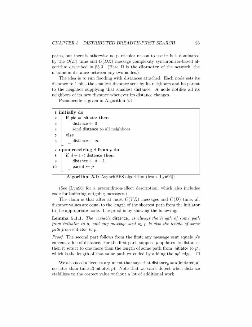
CHAPTER 5. DISTRIBUTED BREADTH-FIRST SEARCH 26
paths, but there is otherwise no particular reason to use it; it is dominatedby the O(D) time and O(DE) message complexity synchronizer-based al-gorithm described in §5.3. (Here D is the diameter of the network, themaximum distance between any two nodes.)
The idea is to run flooding with distances attached. Each node sets itsdistance to 1 plus the smallest distance sent by its neighbors and its parentto the neighbor supplying that smallest distance. A node notifies all itsneighbors of its new distance whenever its distance changes.
Pseudocode is given in Algorithm 5.1
1 initially do2 if pid = initiator then3 distance← 04 send distance to all neighbors5 else6 distance←∞
7 upon receiving d from p do8 if d+ 1 < distance then9 distance← d+ 1
10 parent← p
Algorithm 5.1: AsynchBFS algorithm (from [Lyn96])
(See [Lyn96] for a precondition-effect description, which also includescode for buffering outgoing messages.)
The claim is that after at most O(V E) messages and O(D) time, alldistance values are equal to the length of the shortest path from the initiatorto the appropriate node. The proof is by showing the following:Lemma 5.1.1. The variable distancep is always the length of some pathfrom initiator to p, and any message sent by p is also the length of somepath from initiator to p.Proof. The second part follows from the first; any message sent equals p’scurrent value of distance. For the first part, suppose p updates its distance;then it sets it to one more than the length of some path from initiator to p′,which is the length of that same path extended by adding the pp′ edge.
We also need a liveness argument that says that distancep = d(initiator, p)no later than time d(initiator, p). Note that we can’t detect when distancestabilizes to the correct value without a lot of additional work.

CHAPTER 5. DISTRIBUTED BREADTH-FIRST SEARCH 27
In [Lyn96], there’s an extra |V | term in the time complexity that comesfrom message pile-ups, since the model used there only allows one incomingmessage to be processed per time units (the model in [AW04] doesn’t havethis restriction). The trick to arranging this to happen often is to build agraph where node 1 is connected to nodes 2 and 3, node 2 to 3 and 4, node3 to 4 and 5, etc. This allows us to quickly generate many paths of distinctlengths from node 1 to node k, which produces k outgoing messages fromnode k. It may be that a more clever analysis can avoid this blowup, byshowing that it only happens in a few places.
5.2 Using layeringThis approach is used in the LayeredBFS algorithm in [Lyn96], which is dueto Gallager [Gal82].
Here we run a sequence of up to |V | instances of the simple algorithmwith a distance bound on each: instead of sending out just 0, the initiatorsends out (0, bound), where bound is initially 1 and increases at each phase.A process only sends out its improved distance if it is less than bound.
Each phase of the algorithm constructs a partial BFS tree that containsonly those nodes within distance bound of the root. This tree is used toreport back to the root when the phase is complete. For the following phase,notification of the increase in bound increase is distributed only through thepartial BFS tree constructed so far. With some effort, it is possible toprove that in a bidirectional network that this approach guarantees thateach edge is only probed once with a new distance (since distance-1 nodesare recruited before distance-2 nodes and so on), and the bound-update andacknowledgment messages contribute at most |V | messages per phase. Sowe get O(E + V D) total messages. But the time complexity is bad: O(D2)in the worst case.
5.3 Using local synchronizationThe reason the layering algorithm takes so long is that at each phase wehave to phone all the way back up the tree to the initiator to get permissionto go on to the next phase. We need to do this to make sure that a nodeis only recruited into the tree once: otherwise we can get pile-ups on thechannels as in the simple algorithm. But we don’t necessarily need to dothis globally. Instead, we’ll require each node at distance d to delay sendingout a recruiting message until it has confirmed that none of its neighbors

CHAPTER 5. DISTRIBUTED BREADTH-FIRST SEARCH 28
will be sending it a smaller distance. We do this by having two classes ofmessages:1
• exactly(d): “I know that my distance is d.”
• more-than(d): “I know that my distance is > d.”
The rules for sending these messages for a non-initiator are:
1. I can send exactly(d) as soon as I have received exactly(d− 1) from atleast one neighbor and more-than(d− 2) from all neighbors.
2. I can sendmore-than(d) if d = 0 or as soon as I have receivedmore-than(d−1) from all neighbors.
The initiator sends exactly(0) to all neighbors at the start of the protocol(these are the only messages the initiator sends).
My distance will be the unique distance that I am allowed to send in anexactly(d) messages. Note that this algorithm terminates in the sense thatevery node learns its distance at some finite time.
If you read the discussion of synchronizers in Chapter 13, this algo-rithm essentially corresponds to building the alpha synchronizer into thesynchronous BFS algorithm, just as the layered model builds in the betasynchronizer. See [AW04, §11.3.2] for a discussion of BFS using synchro-nizers. The original approach of applying synchronizers to get BFS is dueto Awerbuch [Awe85].
We now show correctness. Under the assumption that local computationtakes zero time and message delivery takes at most 1 time unit, we’ll showthat if d(initiator, p) = d, (a) p sends more-than(d′) for any d′ < d by timed′, (b) p sends exactly(d) by time d, (c) p never sends more-than(d′) for anyd′ ≥ d, and (d) p never sends exactly(d′) for any d′ 6= d. For parts (c) and(d) we use induction on d′; for (a) and (b), induction on time. This is notterribly surprising: (c) and (d) are safety properties, so we don’t need totalk about time. But (a) and (b) are liveness properties so time comes in.
Let’s start with (c) and (d). The base case is that the initiator neversends any more-than messages at all, and so never sends more-than(0), andany non-initiator never sends exactly(0). For larger d′, observe that if anon-initiator p sends more-than(d′) for d′ ≥ d, it must first have received
1In an earlier version of these notes, these messages where called distance(d) andnot-distance(d); the more self-explanatory exactly and more-than terminology is taken from[BDLP08].

CHAPTER 5. DISTRIBUTED BREADTH-FIRST SEARCH 29
more-than(d′− 1) from all neighbors, including some neighbor p′ at distanced−1. But the induction hypothesis tells us that p′ can’t send more-than(d′−1) for d′ − 1 ≥ d − 1. Similarly, to send exactly(d′) for d′ < d, p must firsthave received exactly(d′− 1) from some neighbor p′, but again p′ must be atdistance at least d−1 from the initiator and so can’t send this message either.In the other direction, to send exactly(d′) for d′ > d, p must first receivemore-than(d′−2) from this closer neighbor p′, but then d′−2 > d−2 ≥ d−1so more-than(d′ − 2) is not sent by p′.
Now for (a) and (b). The base case is that the initiator sends exactly(0)to all nodes at time 0, giving (a), and there is no more-than(d′) with d′ < 0for it to send, giving (b) vacuously; and any non-initiator sends more-than(0)immediately. At time t+ 1, we have that (a) more-than(t) was sent by anynode at distance t + 1 or greater by time t and (b) exactly(t) was sent byany node at distance t by time t; so for any node at distance t + 2 wesend more-than(t+ 1) no later than time t+ 1 (because we already receivedmore-than(t) from all our neighbors) and for any node at distance t + 1 wesend exactly(t + 1) no later than time t + 1 (because we received all thepreconditions for doing so by this time).
Message complexity: A node at distance d sends more-than(d′) for all0 < d′ < d and exactly(d) and no other messages. So we have messagecomplexity bounded by |E| ·D in the worst case. Note that this is gives abound of O(DE), which is slightly worse than the O(E + DV ) bound forthe layered algorithm.
Time complexity: It’s immediate from (a) and (b) that all messages thatare sent are sent by time D, and indeed that any node p learns its distanceat time d(initiator, p). So we have optimal time complexity, at the cost ofhigher message complexity. I don’t know if this trade-off is necessary, or ifa more sophisticated algorithm could optimize both.
Our time proof assumes that messages don’t pile up on edges, or thatsuch pile-ups don’t affect delivery time (this is the default assumption usedin [AW04]). A more sophisticated proof could remove this assumption.
One downside of this algorithm is that it has to be started simultane-ously at all nodes. Alternatively, we could trigger “time 0” at each nodeby a broadcast from the initiator, using the usual asynchronous broadcastalgorithm; this would give us a BFS tree in O(|E| ·D) messages (since theO(|E|) messages of the broadcast disappear into the constant) and 2D time.The analysis of time goes through as before, except that the starting time 0becomes the time at which the last node in the system is woken up by thebroadcast. Further optimizations are possible; see, for example, the paperof Boulinier et al. [BDLP08], which shows how to run the same algorithm

CHAPTER 5. DISTRIBUTED BREADTH-FIRST SEARCH 30
with constant-size messages.

Chapter 6
Leader election
See [AW04, Chapter 3] or [Lyn96, Chapter 3] for details.The basic idea of leader election is that we want a single process to
declare itself leader and the others to declare themselves non-leaders. Thenon-leaders may or may not learn the identity of the leader as part of the pro-tocol; if not, we can always add an extra phase where the leader broadcastsits identity to the others. Traditionally, leader election has been used as away to study the effects of symmetry, and many leader election algorithmsare designed for networks in the form of a ring.
A classic result of Angluin [Ang80] shows that leader election in a ringis impossible if the processes do not start with distinct identities. The proofis that if everybody is in the same state at every step, they all put on thecrown at the same time. We discuss this result in more detail in §6.1.
With ordered identities, a simple algorithm due to Le Lann [LL77] andChang and Roberts [CR79] solves the problem in O(n) time with O(n2)messages: I send out my own id clockwise and forward any id bigger thanmine. If I get my id back, I win. This works with a unidirectional ring,doesn’t require synchrony, and never produces multiple leaders. See §6.2.1for more details.
On a bidirectional ring we can get O(n logn) messages and O(n) timewith power-of-2 probing, using an algorithm of Hirschberg and Sinclair [HS80].This is described in §6.2.2.
An evil trick: if we have synchronized starting, known n, and known idspace, we can have process with id i wait until round i · n to start sendingits id around, and have everybody else drop out when they receive it; thisway only one process (the one with smallest id) ever starts a message andonly n messages are sent [FL87]. But the running time can be pretty bad.
31

CHAPTER 6. LEADER ELECTION 32
For general networks, we can apply the same basic strategy as in LeLann-Chang-Roberts by having each process initiate a broadcast/convergecastalgorithm that succeeds only if the initiator has the smallest id. This isdescribed in more detail in §6.3.
Some additional algorithms for the asynchronous ring are given in §§6.2.3and 6.2.4. Lower bounds are shown in §6.4.
6.1 SymmetryA system exhibits symmetry if we can permute the nodes without changingthe behavior of the system. More formally, we can define a symmetry as anequivalence relation on processes, where we have the additional propertiesthat all processes in the same equivalence class run the same code; andwhenever p is equivalent to p′, each neighbor q of p is equivalent to thecorresponding neighbor q′ of p′.
An example of a network with a lot of symmetries would be an anony-mous ring, which is a network in the form of a cycle (the ring part) inwhich every process runs the same code (the anonymous part). In this caseall nodes are equivalent. If we have a line, then we might or might not haveany non-trivial symmetries: if each node has a sense of direction thattells it which neighbor is to the left and which is to the right, then we canidentify each node uniquely by its distance from the left edge. But if thenodes don’t have a sense of direction,1 we can flip the line over and pair upnodes that map to each other.
Symmetries are convenient for proving impossibility results, as observedby Angluin [Ang80]. The underlying theme is that without some mecha-nism for symmetry breaking, a message-passing system escape from asymmetric initial configuration. The following lemma holds for determin-istic systems, basically those in which processes can’t flip coins:
Lemma 6.1.1. A symmetric deterministic message-passing system thatstarts in an initial configuration in which equivalent processes have the samestate has a synchronous execution in which equivalent processes continue tohave the same state.
Proof. Easy induction on rounds: if in some round p and p′ are equivalentand have the same state, and all their neighbors are equivalent and have thesame state, then p and p′ receive the same messages from their neighbors
1Typically, this means that the nodes can tell their neighbors apart, but that theircode behaves the same way if the left and right neighbors are flipped.

CHAPTER 6. LEADER ELECTION 33
and can proceed to the same state (including outgoing messages) in the nextround.
An immediate corollary is that you can’t do leader election in an anony-mous system with a symmetry that puts each node in a non-trivial equiva-lence class, because as soon as I stick my hand up to declare I’m the leader,so do all my equivalence-class buddies.
With randomization, Lemma 6.1.1 doesn’t directly apply, since we canbreak symmetry by having my coin-flips come up differently from yours. Itdoes show that we can’t guarantee convergence to a single leader in any fixedamount of time (because otherwise we could just fix all the coin flips to geta deterministic algorithm). Depending on what the processes know aboutthe size of the system, it may still be possible to show that a randomizedalgorithm necessarily fails in some cases.
A more direct way to break symmetry is to assume that all processeshave identities; now processes can break symmetry by just declaring thatthe one with the smaller or larger identity wins. This approach is taken inthe algorithms in the following sections.
6.2 Leader election in ringsHere we’ll describe some basic leader election algorithms for rings. Histor-ically, rings were the first networks in which leader election was studied,because they are the simplest networks whose symmetry makes the problemdifficult, and because of the connection to token-ring networks, a methodfor congestion control in local-area networks that is no longer used much.
6.2.1 The Le-Lann-Chang-Roberts algorithm
.This is about the simplest leader election algorithm there is. It works
in a unidirectional ring, where messages can only travel clockwise.2 Thealgorithms works does not require synchrony, but we’ll assume synchrony tomake it easier to follow.
Formally, we’ll let the state space for each process i consist of two vari-ables: leader, initially 0, which is set to 1 if i decides it’s a leader; and maxId,the largest id seen so far. We assume that i denotes i’s position rather than
2We’ll see later in §6.2.3 that the distinction between unidirectional rings and bidirec-tional rings is not a big deal, but for now let’s imagine that having a unidirectional ringis a serious hardship.

CHAPTER 6. LEADER ELECTION 34
its id, which we’ll write as idi. We will also treat all positions as values modn, to simplify the arithmetic.
Code for the LCR algorithm is given in Algorithm 6.1.
1 initially do2 leader← 03 maxId← idi4 send idi to clockwise neighbor5 upon receiving j do6 if j = idi then7 leader← 18 if j > maxId then9 maxId← j
10 send j to clockwise neighbor
Algorithm 6.1: LCR leader election
6.2.1.1 Proof of correctness for synchronous executions
By induction on the round number k. The induction hypothesis is thatin round k, each process i’s leader bit is 0, its maxId value is equal to thelargest id in the range (i−k) . . . i, and that it sends idi−k if and only if idi−kis the largest id in the range (i− k) . . . i. The base case is that when k = 0,maxId = idi is the largest id in i . . . i, and i sends idi. For the induction step,observe that in round k− 1, i− 1 sends id(i−1)−(k−1) = idi−k if and only if itis the largest in the range (i− k) . . . (i− 1), and that i adopts it as the newvalue of maxId and sends it just in case it is larger than the previous largestvalue in (i− k + 1) . . . (i− 1), i.e., if it is the largest value in (i− k) . . . i.
Finally, in round n − 1, i − 1 sends idi−N = idi if and only if i is thelargest id in (i−n+ 1) . . . i, the whole state space. So i receives idi and setsleaderi = 1 if and only if it has the maximum id.
6.2.1.2 Performance
It’s immediate from the correctness proof that the protocols terminates afterexactly n rounds.
To count message traffic, observe that each process sends at most 1message per round, for a total of O(n2) messages. This is a tight bound

CHAPTER 6. LEADER ELECTION 35
since if the ids are in decreasing order n, n− 1, n− 2, . . . 1, then no messagesget eaten until they hit n.
6.2.2 The Hirschberg-Sinclair algorithm
Basically the same as for LCR but both the protocol and the invariantget much messier. To specify the protocol, it may help to think of mes-sages as mobile agents and the state of each process as being of the form(local-state, agents I’m carrying). Then the sending rule for a process be-comes ship any agents in whatever direction they want to go and the tran-sition rule is accept any incoming agents and update their state in terms oftheir own internal transition rules. An agent state for LCR will be some-thing like (original-sender, direction, hop-count, max-seen) where directionis R or L depending on which way the agent is going, hop-count is initially2k when the agent is sent and drops by 1 each time the agent moves, andmax-seen is the biggest id of any node the agent has visited. An agent turnsaround (switches direction) when hop-count reaches 0.
To prove this works, we can mostly ignore the early phases (though wehave to show that the max-id node doesn’t drop out early, which is nottoo hard). The last phase involves any surviving node probing all the wayaround the ring, so it will declare itself leader only when it receives its ownagent from the left. That exactly one node does so is immediate from thesame argument for LCR.
Complexity analysis is mildly painful but basically comes down to thefact that any node that sends a message 2k hops had to be a winner atphase 2k−1, which means that it is the largest of some group of 2k−1 ids.Thus the 2k-hop senders are spaced at least 2k−1 away from each other andthere are at most n/2k−1 of them. Summing up over all dlgne phases, weget
∑dlgnek=0 2kn/2k−1 = O(n logn) messages and
∑dlgnek=0 2k = O(n) time.
6.2.3 Peterson’s algorithm for the unidirectional ring
This algorithm is due to Peterson [Pet82] and assumes an asynchronous,unidirectional ring. It gets O(n logn) message complexity in all executions.
The basic idea (2-way communication version): Start with n candidateleaders. In each of at most lgn asynchronous phases, each candidate probesits nearest neighbors to the left and right; if its ID is larger than the IDs ofboth neighbors, it survives to the next phase. Non-candidates act as relayspassing messages between candidates. As in Hirschberg and Sinclair (§6.2.2),the probing operations in each phase take O(n) messages, and at least half

CHAPTER 6. LEADER ELECTION 36
of the candidates drop out in each phase. The last surviving candidate winswhen it finds that it’s its own neighbor.
To make this work in a 1-way ring, we have to simulate 2-way communi-cation by moving the candidates clockwise around the ring to catch up withtheir unsendable counterclockwise messages. Peterson’s algorithm does thiswith a two-hop approach that is inspired by the 2-way case above; in eachphase k, a candidate effectively moves two positions to the right, allowing itto look at the ids of three phase-k candidates before deciding to continue inphase k+ 1 or not. Here is a very high-level description; it assumes that wecan buffer and ignore incoming messages from the later phases until we getto the right phase, and that we can execute sends immediately upon receiv-ing messages. Doing this formally in terms of I/O automata or the model of§2.1 means that we have to build explicit internal buffers into our processes,which we can easily do but won’t do here (see [Lyn96, pp. 483–484] for theright way to do this.)
We can use a similar trick to transform any bidirectional-ring algorithminto a unidirectional-ring algorithm: alternative between phases where wesend a message right, then send a virtual process right to pick up any left-going messages deposited for us. The problem with this trick is that itrequires two messages per process per phase, which gives us a total messagecomplexity of O(n2) if we start with an O(n)-time algorithm. Peterson’salgorithm avoids this by only propagating the surviving candidates.
Pseudocode for Peterson’s algorithm is given in Algorithm 6.2.Note: the phase arguments in the probe messages are useless if one has
FIFO channels, which is why [Lyn96] doesn’t use them. Note also that thealgorithm does not elect the process with the highest ID, but the processthat is carrying the sole surviving candidate in the last phase.
Proof of correctness is essentially the same as for the 2-way algorithm.For any pair of adjacent candidates, at most one of their current IDs survivesto the next phase. So we get a sole survivor after lgn phases. Each processsends or relays at most 2 messages per phases, so we get at most 2n lgntotal messages.
6.2.4 A simple randomized O(n log n)-message algorithm
An alternative to running a more sophisticated algorithm is to reduce theaverage cost of LCR using randomization. The presentation here follows theaverage-case analysis done by Chang and Roberts [CR79].
Run LCR where each id is constructed by prepending a long randombit-string to the real id. This gives uniqueness (since the real id’s act as

CHAPTER 6. LEADER ELECTION 37
1 procedure candidate()2 phase← 03 current← pid4 while true do5 send probe(phase, current)6 wait for probe(phase, x)7 id2 ← x8 send probe(phase, current)9 wait for probe(phase, x)
10 id3 ← x11 if id2 = current then12 I am the leader!13 return14 else if id2 > current and id2 > id3 do15 current← id216 phase← phase + 117 else18 switch to relay()
19 procedure relay()20 upon receiving probe(p, i) do21 send probe(p, i)
Algorithm 6.2: Peterson’s leader-election algorithm

CHAPTER 6. LEADER ELECTION 38
tie-breakers) and something very close to a random permutation on theconstructed id’s. When we have unique random id’s, a simple argumentshows that the i-th largest id only propagates an expected n/i hops, givinga total of O(nHn) = O(n logn) hops.3 Unique random id’s occur with highprobability provided the range of the random sequence is n2.
The downside of this algorithm compared to Peterson’s is that knowledgeof n is required to pick random id’s from a large enough range. It also hashigher bit complexity since Peterson’s algorithm is sending only IDs (in theofficial version) without any random padding.
6.3 Leader election in general networksFor general networks, a simple approach is to have each node initiate abreadth-first-search and convergecast, with nodes refusing to participate inthe protocol for any initiator with a lower id. It follows that only the nodewith the maximum id can finish its protocol; this node becomes the leader.If messages from parallel broadcasts are combined, it’s possible to keep themessage complexity of this algorithm down to O(DE).
More sophisticated algorithms reduce the message complexity by coalesc-ing local neighborhoods similar to what happens in the Hirschberg-Sinclairand Peterson algorithms. A noteworthy example is an O(n logn) message-complexity algorithm of Afek and Gafni [AG91], who also show an Ω(n logn)lower bound on message complexity for any synchronous algorithm in a com-plete network.
6.4 Lower boundsHere we present two classic Ω(logn) lower bounds on message complexityfor leader election in the ring. The first, due to Burns [Bur80], assumesthat the system is asynchronous and that the algorithm is uniform: itdoes not depend on the size of the ring. The second, due to Fredericksonand Lynch [FL87], allows a synchronous system and relaxes the uniformityassumption, but requires that the algorithm can’t do anything to ids butcopy and compare them.
3Alternatively, we could consider the average-case complexity of the algorithm whenwe assume all n! orderings of the ids are equally likely; this also gives O(n logn) expectedmessage complexity [CR79].

CHAPTER 6. LEADER ELECTION 39
6.4.1 Lower bound on asynchronous message complexity
Here we describe a lower bound for uniform asynchronous leader election inthe ring. The description here is based on [AW04, §3.3.3]; a slightly differentpresentation can also be found in [Lyn96, §15.1.4]. The original result is dueto Burns [Bur80]. We assume the system is deterministic.
The basic idea is to construct a bad execution in which n processessend lots of messages recursively, by first constructing two bad (n/2)-processexecutions and pasting them together in a way that generates many extramessages. If the pasting step produces Θ(n) additional messages, we get arecurrence T (n) ≥ 2T (n/2) + Θ(n) for the total message traffic, which hassolution T (n) = Ω(n logn).
We’ll assume that all processes are trying to learn the identity of theprocess with the smallest id. This is a slightly stronger problem that mereleader election, but it can be solved with at most an additional 2n messagesonce we actually elect a leader. So if we get a lower bound of f(n) messageson this problem, we immediately get a lower bound of f(n) − 2n on leaderelection.
To construct the bad execution, we consider “open executions” on ringsof size n where no message is delivered across some edge (these will be partialexecutions, because otherwise the guarantee of eventual delivery kicks in).Because no message is delivered across this edge, the processes can’t tell ifthere is really a single edge there or some enormous unexplored fragment ofa much larger ring. Our induction hypothesis will show that a line of n/2processes can be made to send at least T (n/2) messages in an open execution(before seeing any messages across the open edge); we’ll then show that alinear number of additional messages can be generated by pasting two suchexecutions together end-to-end, while still getting an open execution with nprocesses.
In the base case, we let n = 2. Somebody has to send a message even-tually, giving T (2) ≥ 1.
For larger n, suppose that we have two open executions on n/2 processesthat each send at least T (n/2) messages. Break the open edges in bothexecutions and paste the resulting lines together to get a ring of size n;similarly paste the schedules σ1 and σ2 of the two executions together toget a combined schedule σ1σ2 with at least 2T (n/2) messages. Note that inthe combined schedule no messages are passed between the two sides, so theprocesses continue to behave as they did in their separate executions.
Let e and e′ be the edges we used to past together the two rings. Extendσ1σ2 by the longest possible suffix σ3 in which no messages are delivered

CHAPTER 6. LEADER ELECTION 40
across e and e′. Since σ3 is as long as possible, after σ1σ2σ3, there are nomessages waiting to be delivered across any edge except e and e′ and allprocesses are quiescent—they will send no additional messages until theyreceive one.
Now consider the processes in the half of the ring with the larger min-imum id. Because each process must learn the minimum id in the otherhalf of the ring, each of these processes must receive a message in somecomplete execution, giving an additional n/2− 2 messages (since two of theprocesses might receive undelivered messages on e or e′ that we’ve alreadycounted). But to prove our induction hypothesis, we need to keep one ofe or e′ open. Consider some execution σ1σ2σ3σ4 in which all messages de-layed on both e and e′ are delivered, and partition the n/2 process on thelosing side into two groups based on whether the first message they get istriggered by opening e or e′. One of these two groups must contain at leasthalf the n/2− 2 processes who receive new messages, meaning that there isan execution σ1σ2σ3σ
′4 in which we open up only one edge and still get an
additional (n/2− 2)/2 = Θ(n) messages. This concludes the proof.
6.4.2 Lower bound for comparison-based algorithms
Here we give an Ω(n logn) lower bound on messages for synchronous-startcomparison-based algorithms in bidirectional synchronous rings. For fulldetails see [Lyn96, §3.6], [AW04, §3.4.2], or the original JACM paper byFrederickson and Lynch [FL87].
Basic ideas:
• Two fragments i . . . i+k and j . . . j+k of a ring are order-equivalentprovided idi+a > idi+b if and only if idj+a > idj+b for b = 0 . . . k.
• An algorithm is comparison-based if it can’t do anything to IDsbut copy them and test for <. The state of such an algorithm ismodeled by some non-ID state together with a big bag of IDs, messageshave a pile of IDs attached to them, etc. Two states/messages areequivalent under some mapping of IDs if you can translate the firstto the second by running all IDs through the mapping. Alternateversion: Executions of p1 and p2 are similar if they send messages inthe same direction(s) in the same rounds, declare themselves leaderat the same round; an algorithm is comparison-based based if order-equivalent rings yield similar executions for corresponding processes.This can be turned into the explicit-copying-IDs model by replacingthe original protocol with a full-information protocol in which each

CHAPTER 6. LEADER ELECTION 41
message is replaced by the ID and a complete history of the sendingprocess (including all messages it has every received).
• Define an active round as a round in which at least 1 message issent. Claim: actions of i after k active rounds depends up to an order-equivalent mapping of ids only on the order-equivalence class of idsin i − k . . . i + k (the k-neighborhood of i). Proof: by induction onk. Suppose i and j have order-equivalent (k− 1)-neighborhoods; thenafter k − 1 active rounds they have equivalent states by the induc-tion hypothesis. In inactive rounds, i and j both receive no messagesand update their states in the same way. In active rounds, i and jreceive order-equivalent messages and update their states in an order-equivalent way.
• If we have an order of ids with a lot of order-equivalent k-neighborhoods,then after k active rounds if one process sends a message, so do a lotof other ones.
Now we just need to build a ring with a lot of order-equivalent neighbor-hoods. For n a power of 2 we can use the bit-reversal ring, e.g., id sequence000, 100, 010, 110, 001, 101, 011, 111 (in binary) when n = 8. Figure 6.1 givesa picture of what this looks like for n = 32.
For n not a power of 2 we look up Frederickson and Lynch [FL87] or At-tiya et al. [ASW88]. In either case we get Ω(n/k) order-equivalent membersof each equivalence class after k active rounds, giving Ω(n/k) messages peractive round, which sums to Ω(n logn).
For non-comparison-based algorithms we can still prove Ω(n logn) mes-sages for time-bounded algorithms, but it requires techniques from Ram-sey theory, the branch of combinatorics that studies when large enoughstructures inevitably contain substructures with certain properties.4 Here“time-bounded” means that the running time can’t depend on the size ofthe ID space. See [AW04, §3.4.2] or [Lyn96, §3.7] for the textbook version,or [FL87, §7] for the original result.
The intuition is that for any fixed protocol, if the ID space is largeenough, then there exists a subset of the ID space where the protocol
4The classic example is Ramsey’s Theorem, which says that if you color the edgesof a complete graph red or blue, while trying to avoid having any subsets of k verticeswith all edges between them the same color, you will no longer be able to once the graphis large enough (for any fixed k). See [GRS90] for much more on the subject of Ramseytheory.

CHAPTER 6. LEADER ELECTION 42
0
5
10
15
20
25
30
35
-5 0 5 10 15 20 25 30 35
Figure 6.1: Labels in the bit-reversal ring with n = 32
acts like a comparison-based protocol. So the existence of an O(f(n))-message time-bounded protocol implies the existence of an O(f(n))-messagecomparison-based protocol, and from the previous lower bound we knowf(n) is Ω(n logn). Note that time-boundedness is necessary: we can’t provethe lower bound for non-time-bounded algorithms because of the i · n trick.

Chapter 7
Synchronous agreement
Here we’ll consider synchronous agreement algorithm with stopping failures,where a process stops dead at some point, sending and receiving no furthermessages. We’ll also consider Byzantine failures, where a process deviatesfrom its programming by sending arbitrary messages, but mostly just to seehow crash-failure algorithms hold up; for algorithms designed specifically fora Byzantine model, see Chapter 8.
If the model has communication failures instead, we have the coordinatedattack problem from Chapter 3.
7.1 Problem definitionWe use the usual synchronous model with n processes with binary inputsand binary outputs. Up to f processes may fail at some point; when aprocess fails, one or one or more of its outgoing messages are lost in theround of failure and all outgoing messages are lost thereafter.
There are two variants on the problem, depending on whether we wanta useful algorithm (and so want strong conditions to make our algorithmmore useful) or a lower bound (and so want weak conditions to make ourlower bound more general). For algorithms, we will ask for these conditionsto hold:
Agreement All non-faulty processes decide the same value.
Validity If all processes start with the same input, all non-faulty processesdecide it.
Termination All non-faulty processes eventually decide.
43

CHAPTER 7. SYNCHRONOUS AGREEMENT 44
For lower bounds, we’ll replace validity with non-triviality (often calledvalidity in the literature):
Non-triviality There exist failure-free executions A and B that producedifferent outputs.
Non-triviality follows from validity but doesn’t imply validity; for exam-ple, a non-trivial algorithm might have the property that if all non-faultyprocesses start with the same input, they all decide something else. We’llstart by using non-triviality, agreement, and termination to show a lowerbound on the number of rounds needed to solve the problem.
7.2 Lower bound on roundsHere we show that synchronous agreement requires at least f + 1 roundsif f processes can fail. This proof is modeled on the one in [Lyn96, §6.7]and works backwards from the final state; for a proof of the same resultthat works in the opposite direction, see [AW04, §5.1.4]. The original result(stated for Byzantine failures) is due to Dolev and Strong [DS83], based ona more complicated proof due to Fischer and Lynch [FL82]; see the chapternotes for Chapter 5 of [AW04] for more discussion of the history.
Like the similar proof for coordinated attack (§3.2), the proof uses anindistinguishability argument. But we have to construct a more complicatedchain of intermediate executions.
A crash failure at process i means that (a) in some round r, some orall of the messages sent by i are not delivered, and (b) in subsequent rounds,no messages sent by i are delivered. The intuition is that i keels over deadin the middle of generating its outgoing messages for a round. Otherwise ibehaves perfectly correctly. A process that crashes at some point during anexecution is called faulty
We will show that if up to f processes can crash, and there are at leastf + 2 processes, then at least f + 1 rounds are needed (in some execution)for any algorithm that satisfies agreement, termination, and non-triviality.In particular, we will show that if all executions run in f or fewer rounds,then the indistinguishability graph is connected; this implies non-trivialitydoesn’t hold, because (as in §3.2), two adjacent states must decide the samevalue because of the agreement property.1
1The same argument works with even a weaker version of non-triviality that omits therequirement that A and B are failure-free, but we’ll keep things simple.

CHAPTER 7. SYNCHRONOUS AGREEMENT 45
Now for the proof. To simplify the argument, let’s assume that all ex-ecutions terminate in exactly f rounds (we can always have processes sendpointless chitchat to pad out short executions) and that every processessends a message to every other process in every round where it has notcrashed (more pointless chitchat). Formally, this means we have a sequenceof rounds 0, 1, 2, . . . , f−1 where each process sends a message to every otherprocess (assuming no crashes), and a final round f where all processes decideon a value (without sending any additional messages).
We now want to take any two executions A and B and show that bothproduce the same output. To do this, we’ll transform A’s inputs into B’sinputs one process at a time, crashing processes to hide the changes. Theproblem is that just crashing the process whose input changed might changethe decision value—so we have to crash later witnesses carefully to maintainindistinguishability all the way across the chain.
Let’s say that a process p crashes fully in round r if it crashes in roundr and no round-r messages from p are delivered. The communicationpattern of an execution describes which messages are delivered betweenprocesses without considering their contents—in particular, it tells us whichprocesses crash and what other processes they manage to talk to in theround in which they crash.
With these definitions, we can state and prove a rather complicatedinduction hypothesis:
Lemma 7.2.1. For any f -round protocol with n ≥ f + 2 process permittingup to f crash failures; any process p; and any execution A in which atmost one processes crashes per round in rounds 0 . . . r−1, p crashes fully inround r + 1, and no other processes crash; there is a sequence of executionsA = A0A1 . . . Ak such that each Ai is indistinguishable from Ai+1 by someprocess, each Ai has at most one crash per round, and the communicationpattern in Ak is identical to A except that p crashes fully in round r.
Proof. By induction on f − r. If r = f , we just crash p in round r andnobody else notices. For r < f , first crash p in round r instead of r+ 1, butdeliver all of its round-r messages anyway (this is needed to make space forsome other process to crash in round r + 1). Then choose some message msent by p in round r, and let p′ be the recipient of m. We will show that wecan produce a chain of indistinguishable executions between any executionin which m is delivered and the corresponding execution in which it is not.
If r = f − 1, this is easy; only p′ knows whether m has been delivered,and since n ≥ f+2, there exists another non-faulty p′′ that can’t distinguishbetween these two executions, since p′ sends no messages in round f or later.

CHAPTER 7. SYNCHRONOUS AGREEMENT 46
If r < f −1, we have to make sure p′ doesn’t tell anybody about the missingmessage.
By the induction hypothesis, there is a sequence of executions startingwith A and ending with p′ crashing fully in round r+ 1, such that each exe-cution is indistinguishable from its predecessor. Now construct the sequence
A→ (A with p′ crashing fully in r + 1)→ (A with p′ crashing fully in r + 1 and m lost)→ (A with m lost and p′ not crashing).
The first and last step apply the induction hypothesis; the middle one yieldsindistinguishable executions since only p′ can tell the difference between marriving or not and its lips are sealed.
We’ve shown that we can remove one message through a sequence ofexecutions where each pair of adjacent executions is indistinguishable tosome process. Now paste together n − 1 such sequences (one per message)to prove the lemma.
The rest of the proof: Crash some process fully in round 0 and thenchange its input. Repeat until all inputs are changed.
7.3 SolutionsHere we give two solutions to synchronous agreement with crash failures.The first, due to Dolev and Strong [DS83], is more practical but does not gen-eralize well to Byzantine failures. The second is a variant on the exponentialinformation gathering algorithm of Pease, Shostak, and Lamport [PSL80],which propagates enough information that it can in principle simulate anyother possible algorithm; it is mostly of interest because it can be used forthe Byzantine case as well.
7.3.1 Flooding
We’ll now show an algorithm that gets agreement, termination, and validity.Validity here is stronger than the non-triviality condition used in the lowerbound, but the lower bound still applies: we can’t do this in less than f + 1rounds.
So let’s do it in exactly f+1 rounds. There are two standard algorithms,one of which generalizes to Byzantine processes under good conditions. We’llstart with a simple approach based on flooding. This algorithm is described

CHAPTER 7. SYNCHRONOUS AGREEMENT 47
in more detail in [AW04, §5.1.3] or [Lyn96, §6.2.1]; the original is due toDolev and Strong [DS83].
Assumes very trustworthy processes. Each process keeps a set of (pro-cess, input) pairs, initially just (myId,myInput). At round r, I broadcastmy set to everybody and take the union of my set and all sets I receive.At round f + 1, I decide on f(S), where f is some fixed function from setsof process-input pairs to outputs that picks some input in S: for example,f might take the input with the smallest process-id attached to it, takethe max of all known input values, or take the majority of all known inputvalues.
Lemma 7.3.1. After f + 1 rounds, all non-faulty processes have the sameset.
Proof. Let Sri be the set of process i after r rounds. What we’ll really showis that if there are no failures in round k, then Sri = Srj = Sk+1
i for all i,j, and r > k. To show this, observe that no faults in round k means thatall processes that are still alive at the start of round k send their messageto all other processes. Let L be the set of live processes in round k. At theend of round k, for i in L we have Sk+1
i =⋃j∈L S
kj = S. Now we’ll consider
some round r = k + 1 + m and show by induction on m that Sk+mi = S;
we already did m = 0, so for larger m notice that all messages are equalto S and so Sk+1+m
i is the union of a whole bunch of S’s. So in particularwe have Sf+1
i = S (since some failure-free round occurred in the precedingf + 1 rounds) and everybody decides the same value f(S).
Flooding depends on being able to trust second-hand descriptions ofvalues; it may be that process 1 fails in round 0 so that only process 2 learnsits input. If process 2 can suddenly tell 3 (but nobody else) about the inputin round f + 1—or worse, tell a different value to 3 and 4—then we mayget disagreement. This remains true even if Byzantine processes can’t fakeinputs (e.g., because an input value is really a triple (i, v, signature(v)) usingan unforgeable digital signature)—the reason is that a Byzantine processcould horde some input (i, v, signature(v)) until the very last round and thendeliver it to only some of the non-faulty processes.
7.4 Exponential information gatheringThe idea of exponential information gathering is that each processwill do a lot of gossiping, but now its state is no longer just a flat set of

CHAPTER 7. SYNCHRONOUS AGREEMENT 48
inputs, but a tree describing who it heard what from. We build this treeout of pairs of the form (id-sequence, input) where id-sequence is a sequenceof intermediaries with no repetitions and input is some input. A process’sstate at each round is just a set of such pairs.
This is not really an improvement on flooding for crash failures, but itcan be used as a basis for building an algorithm for Byzantine agreement(Chapter 8). Also useful as an example of a full-information algorithm,in which every process records all that it knows about the execution; inprinciple this allows the algorithm to simulate any other algorithm, whichcan sometimes be useful for proving lower bounds.
See [AW04, §5.2.4] or [Lyn96, §6.2.3] for more details than we providehere. The original exponential information-gathering algorithm (for Byzan-tine processes) is due to Pease, Shostak, and Lamport [PSL80].
Initial state is (〈〉,myInput).At round r, process i broadcasts all pairs (w, v) where |w| = r and i
does not appear in w (these restrictions make the algorithm slightly lessexponential). Upon receiving (w, v) from j, i adds (wj, v) to its list. If nomessage arrives from j in round r, i adds (wj,⊥) to its list for all non-repeating w with |w| = r (this step can also be omitted).
A tree structure is obtained by letting w be the parent of wj for each j.At round f + 1, apply some fixed decision rule to the set of all values
that appear in the tree (e.g. take the max, or decide on a default value v0if there is more than one value in the tree). That this works follows prettymuch immediately from the fact that the set of node labels propagates justas in the flooding algorithm (which is why EIG isn’t really an improvement).But there are some complications from the messages that aren’t sent due tothe i-not-in-w restriction on sending. So we have to write out a real proof.Below is basically just following the presentation in [Lyn96].
Let val(w, i) be the value v such that (w, v) appears in i’s list at theend of round f + 1. We don’t worry about what earlier round it appears inbecause we can compute that round as |w|+ 1.
7.4.1 Basic invariants
• val(〈〉, i) = i’s input.
• Either val(wj, i) equals val(w, j) or val(wj, i) = ⊥ and j didn’t send amessage in round |w|+ 1.
These are trivial.
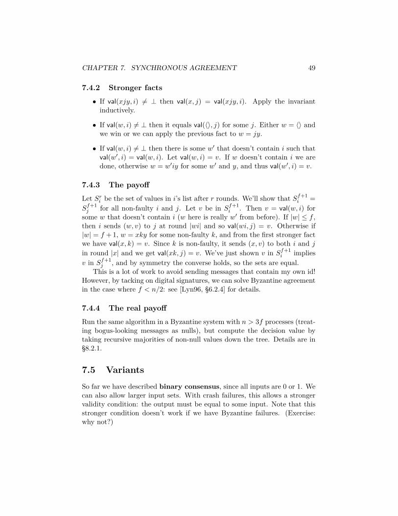
CHAPTER 7. SYNCHRONOUS AGREEMENT 49
7.4.2 Stronger facts
• If val(xjy, i) 6= ⊥ then val(x, j) = val(xjy, i). Apply the invariantinductively.
• If val(w, i) 6= ⊥ then it equals val(〈〉, j) for some j. Either w = 〈〉 andwe win or we can apply the previous fact to w = jy.
• If val(w, i) 6= ⊥ then there is some w′ that doesn’t contain i such thatval(w′, i) = val(w, i). Let val(w, i) = v. If w doesn’t contain i we aredone, otherwise w = w′iy for some w′ and y, and thus val(w′, i) = v.
7.4.3 The payoff
Let Sri be the set of values in i’s list after r rounds. We’ll show that Sf+1i =
Sf+1j for all non-faulty i and j. Let v be in Sf+1
i . Then v = val(w, i) forsome w that doesn’t contain i (w here is really w′ from before). If |w| ≤ f ,then i sends (w, v) to j at round |wi| and so val(wi, j) = v. Otherwise if|w| = f + 1, w = xky for some non-faulty k, and from the first stronger factwe have val(x, k) = v. Since k is non-faulty, it sends (x, v) to both i and jin round |x| and we get val(xk, j) = v. We’ve just shown v in Sf+1
i impliesv in Sf+1
j , and by symmetry the converse holds, so the sets are equal.This is a lot of work to avoid sending messages that contain my own id!
However, by tacking on digital signatures, we can solve Byzantine agreementin the case where f < n/2: see [Lyn96, §6.2.4] for details.
7.4.4 The real payoff
Run the same algorithm in a Byzantine system with n > 3f processes (treat-ing bogus-looking messages as nulls), but compute the decision value bytaking recursive majorities of non-null values down the tree. Details are in§8.2.1.
7.5 VariantsSo far we have described binary consensus, since all inputs are 0 or 1. Wecan also allow larger input sets. With crash failures, this allows a strongervalidity condition: the output must be equal to some input. Note that thisstronger condition doesn’t work if we have Byzantine failures. (Exercise:why not?)

Chapter 8
Byzantine agreement
Like synchronous agreement (as in Chapter 7) except that we replace crashfailures with Byzantine failures, where a faulty process can ignore itsprogramming and send any messages it likes. Since we are operating undera universal quantifier, this includes the case where the Byzantine processesappear to be colluding with each other under the control of a centralizedadversary.
8.1 Lower boundsWe’ll start by looking at lower bounds.
8.1.1 Minimum number of rounds
We’ve already seen an f + 1 lower bound on rounds for crash failures (see§7.2). This lower bound applies a fortiori to Byzantine failures, since Byzan-tine failures can simulate crash failures.
8.1.2 Minimum number of processes
We can also show that we need n > 3f processes. For n = 3 and f = 1 theintuition is that Byzantine B can play non-faulty A and C off against eachother, telling A that C is Byzantine and C that A is Byzantine. Since A istelling C the same thing about B that B is saying about A, C can’t tell thedifference and doesn’t know who to believe. Unfortunately, this tragic soapopera is not a real proof, since we haven’t actually shown that B can sayexactly the right thing to keep A and C from guessing that B is evil.
50

CHAPTER 8. BYZANTINE AGREEMENT 51
A0 B0
C
A0 B0
C0
A1B1
C1
Figure 8.1: Three-process vs. six-process execution in Byzantine agreementlower bound. Processes A0 and B0 in right-hand execution receive samemessages as in left-hand three-process execution with Byzantine C simula-tion C0 through C1. So validity forces them to decide 0. A similar argumentusing Byzantine A shows the same for C0.
The real proof:1 Consider an artificial execution where (non-Byzantine)A, B, and C are duplicated and then placed in a ring A0B0C0A1B1C1,where the digits indicate inputs. We’ll still keep the same code for n = 3on A0, B0, etc., but when A0 tries to send a message to what it thinks ofas just C we’ll send it to C1 while messages from B0 will instead go to C0.For any adjacent pair of processes (e.g. A0 and B0), the behavior of the restof the ring could be simulated by a single Byzantine process (e.g. C), soeach process in the 6-process ring behaves just as it does in some 3-processexecution with 1 Byzantine process. It follows that all of the processesterminate and decide in the unholy 6-process Frankenexecution2 the samevalue that they would in the corresponding 3-process Byzantine execution.So what do they decide?
Given two processes with the same input, say, A0 and B0, the giant exe-cution is indistinguishable from an A0B0C execution where C is Byzantine(see Figure 8.1. Validity says A0 and B0 must both decide 0. Since thisworks for any pair of processes with the same input, we have each processdeciding its input. But now consider the execution of C0A1B, where B isByzantine. In the big execution, we just proved that C0 decides 0 and A1decides 1, but since the C0A1B execution is indistinguishable from the bigexecution to C0 and A1, they do the same thing here and violate agreement.
This shows that with n = 3 and f = 1, we can’t win. We can generalizethis to n = 3f . Suppose that there were an algorithm that solved Byzantineagreement with n = 3f processes. Group the processes into groups of size f ,
1The presentation here is based on [AW04, §5.2.3]. The original impossibility resultis due to Pease, Shostak, and Lamport [PSL80]. This particular proof is due to Fischer,Lynch, and Merritt [FLM86].
2Not a real word.

CHAPTER 8. BYZANTINE AGREEMENT 52
A0
B0
C
D0
A0
B0
D0
C0
A1B1
C1
D1
Figure 8.2: Four-process vs. eight-process execution in Byzantine agreementconnectivity lower bound. Because Byzantine C can simulate C0, D1, B1, A1,and C1, A0, B0 and D0 must all decide 0 or risk violating validity.
and let each of the n = 3 processes simulate one group, with everybody inthe group getting the same input, which can only make things easier. Thenwe get a protocol for n = 3 and f = 1, an impossibility.
8.1.3 Minimum connectivity
So far, we’ve been assuming a complete communication graph. If the graph isnot complete, we may not be able to tolerate as many failures. In particular,we need the connectivity of the graph (minimum number of nodes that mustbe removed to split it into two components) to be at least 2f+1. See [Lyn96,§6.5] for the full proof. The essential idea is that if we have an arbitrarygraph with a vertex cut of size k < 2f + 1, we can simulate it on a 4-processgraph where A is connected to B and C (but not D), B and C are connectedto each other, and D is connected only to B and C. Here B and C eachsimulate half the processes in the size-k cut, A simulates all the processeson one side of the cut and D all the processes on the other side. We thenconstruct an 8-process artificial execution with two non-faulty copies of eachof A, B, C, and D and argue that if one of B or C can be Byzantine thenthe 8-process execution is indistinguishable to the remaining processes froma normal 4-process execution. (See Figure 8.1.)
An argument similar to the n > 3f proof then shows we violate oneof validity or agreement: if we replacing C0, C1, and all the nodes on oneside of the C0 + C1 cut with a single Byzantine C, we force the remainingnon-faulty nodes to decide their inputs or violate validity. But then doing

CHAPTER 8. BYZANTINE AGREEMENT 53
the same thing with B0 and B1 yields an execution that violates agreement.Conversely, if we have connectivity 2f+1, then the processes can simulate
a general graph by sending each other messages along 2f + 1 predeterminedvertex-disjoint paths and taking the majority value as the correct message.Since the f Byzantine processes can only corrupt one path each (assumingthe non-faulty processes are careful about who they forward messages from),we get at least f + 1 good copies overwhelming the f bad copies. Thisreduces the problem on a general graph with sufficiently high connectivityto the problem on a complete graph, allowing Byzantine agreement to besolved if the other lower bounds are met.
8.1.4 Weak Byzantine agreement
(Here we are following [Lyn96, §6.6]. The original result is due to Lam-port [Lam83].)
Weak Byzantine agreement is like regular Byzantine agreement, butvalidity is only required to hold if there are no faulty processes at all.3 Ifthere is a single faulty process, the non-faulty processes can output any valueregardless of their inputs (as long as they agree on it). Sadly, this weakeningdoesn’t improve things much: even weak Byzantine agreement can be solvedonly if n ≥ 3f + 1.
Proof: As in the strong Byzantine agreement case, we’ll construct amany-process Frankenexecution to figure out a strategy for a single Byzan-tine process in a 3-process execution. The difference is that now the numberof processes in our synthetic execution is much larger, since we want tobuild an execution where at least some of our test subjects think they arein a non-Byzantine environment. The trick is to build a very big, highly-symmetric ring so that at least some of the processes are so far away fromthe few points of asymmetry that might clue them in to their odd conditionthat the protocol terminates before they notice.
Fix some protocol that allegedly solves weak Byzantine agreement, andlet r be the number of rounds for the protocol. Construct a ring of 6r pro-cessesA01B01C01A02B02C02 . . . A0rB0rC0rA10B10C10 . . . A1rB1rC1r, where eachXij runs the code for process X in the 3-process protocol with input i. Foreach adjacent pair of processes, there is a 3-process Byzantine execution
3An alternative might be to weaken agreement or termination to apply only if thereare no non-faulty processes, but this makes the problem trivial. If we weaken agreement,we can just have each process decide whatever process 1 tells it to, and if we weakentermination, we can do more or less the same thing except that we only terminate if allthe other processes tell us they heard the same value from process 1.

CHAPTER 8. BYZANTINE AGREEMENT 54
which is indistinguishable from the 6r-process execution for that pair: sinceagreement holds in all Byzantine executions, each adjacent pair decides thesame value in the big execution and so either everybody decides 0 or every-body decides 1 in the big execution.
Now we’ll show that means that validity is violated in some no-failures 3-process execution. We’ll extract this execution by looking at the executionof processes A0r/2B0r/2C0r/2. The argument is that up to round r, anyinput-0 process that is at least r steps in the ring away from the nearest1-input process acts like the corresponding process in the all-0 no-failures3-process execution. Since A0,r/2 is 3r/2 > r hops away from A1r andsimilarly for C0,r/2, our 3 stooges all decide 0 by validity. But now repeatthe same argument for A1,r/2B1,r/2C1,r/2 and get 3 new stooges that alldecide 1. This means that somewhere in between we have two adjacentprocesses where one decides 0 and one decides 1, violating agreement in thecorresponding 3-process execution where the rest of the ring is replaced bya single Byzantine process. This concludes the proof.
This result is a little surprising: we might expect that weak Byzantineagreement could be solved by allowing a process to return a default valueif it notices anything that might hint at a fault somewhere. But this wouldallow a Byzantine process to create disagreement revealing its bad behaviorto just one other process in the very last round of an execution otherwiseheaded for agreement on the non-default value. The chosen victim decidesthe default value, but since it’s the last round, nobody else finds out. Evenif the algorithm is doing something more sophisticated, examining the 6r-process execution will tell the Byzantine process exactly when and how tostart acting badly.
8.2 Upper boundsHere we describe two upper bounds for Byzantine agreement, one of whichgets an optimal number of rounds at the cost of many large messages, andthe other of which gets smaller messages at the cost of more rounds. (Weare following §§5.2.4–5.2.5 of [AW04] in choosing these algorithms.) Neitherof these algorithms is state-of-the-art, but they demonstrate some of theissues in solving Byzantine agreement without the sometimes-complicatedoptimizations needed to get all the parameters of the algorithm down simul-taneously.

CHAPTER 8. BYZANTINE AGREEMENT 55
8.2.1 Exponential information gathering gets n = 3f + 1We’ll show that a variant of Exponential Information Gathering as defined in§7.4 works with n ≥ 3f +1 in f +1 rounds. This is the same technique usedby Pease, Shostak, and Lamport [PSL80] to show that their impossibilityresult is tight.
Recall EIG gives us at each node a set of pairs (path, value) where pathspans all sequences of 0 to n distinct ids and value is the input value for-warded along that path. We write val(w, i) for the value stored in i’s list atthe end of the protocol that is associated with path w. Because we can’ttrust these val(w, i) values to be an accurate description of any process’sinput if there is a Byzantine process in w, each process computes for itselfreplacement values val′(w, i) that use majority voting to try to get a moretrustworthy picture of the original inputs.
Formally, we think of the set of paths as a tree where w is the parent ofwj for each path w and each id j not in w. To apply EIG in the Byzantinemodel, ill-formed messages received from j are treated as missing messages,but otherwise the data-collecting part of EIG proceeds as in the crash failuremodel. However, we compute the decision value from the last-round valuesrecursively as follows. First replace any missing pair involving a path w with|w| = f + 1 with (w, 0). Then for each path w, define val′(w, i) to be themajority value among val′(wj, i) for all j, or val(w, i) if |w| = f + 1. Finally,we have process i decide val′(〈〉, i) (which it can compute locally from itsown stored values val(w, i)).
The val′ is a reconstruction of old values from later ones: as we moveup the tree from wj to w we are moving backwards in time, until in theend we get the decision value val′(〈〉, i) as a majority of reconstructed inputsval′(j, i). One way to think about this is that I don’t trust j to give methe right value for wj—even when w = 〈〉 and j is just reporting its owninput—so instead a take a majority of values of wj that j allegedly reportedto other people. But since I don’t trust those other people either, I use thesame process recursively to construct those reports.
8.2.1.1 Proof of correctness
This is just a sketch of the proof from [Lyn96, §6.3.2]; essentially the sameargument appears in [AW04, §5.2.4].
We start with a basic observation that good processes send and recordvalues correctly:

CHAPTER 8. BYZANTINE AGREEMENT 56
Lemma 8.2.1. If i, j, and k are all non-faulty then for all w, val(wk, i) =val(wk, j) = val(w, k).
Proof. Trivial: k announces the same value val(w, k) to both i and j.
More involved is this lemma, which says that when we reconstruct avalue for a trustworthy process at some level, we get the same value thatit sent us. In particular this will be used to show that the reconstructedinputs val′(j, i) are all equal to the real inputs for good processes.
Lemma 8.2.2. If j is non-faulty then val′(wj, i) = val(wj, i) for all non-faulty i and all w.
Proof. By induction on f + 1 − |wj|. If |wj| = f + 1, then val′(wj, i) =val(wj, i) = val(w, j) = val(wj, i). If |wj| < f +1, then val(wj, k) = val(w, j)for all non-faulty k. It follows that val(wjk, i) = val(w, j) for all non-faultyi and k (that do no appear in w). The bad guys report at most f badvalues val(wj, k′), but the good guys report at least n−f −|wj| good valuesval(wj, k). Since n ≥ 3f + 1 and |wj| ≤ f , we have n− f − |wj| ≥ 3f + 1−f − f ≥ f + 1 good values, which are a majority.
We call a node w common val′(w, i) = val′(w, j) for all non-faulty i, j.Lemma 8.2.2 says that wk is common if k is non-faulty. We can also showthat any node whose children are all common is also common, whether ornot the last process in its label is faulty.
Lemma 8.2.3. Let wk be common for all k. Then w is common.
Proof. Recall that, for |w| < f + 1, val′(w, i) is the majority value amongall val′(wk, i). If all wk are common, then val′(wk, i) = val′(wk, j) for allnon-faulty i and j, so i and j compute the same majority values and getval′(w, i) = val′(w, j).
We can now prove the full result.
Theorem 8.2.4. Exponential information gathering using f + 1 rounds ina synchronous Byzantine system with at most f faulty processes satisfiesvalidity and agreement, provided n ≥ 3f + 1.
Proof. Validity: Immediate application of Lemmas 8.2.1 and 8.2.2 whenw = 〈〉. We have val′(j, i) = val(j, i) = val(〈〉, j) for all non-faulty j and i,which means that a majority of the val′(j, i) values equal the common inputand thus so does val′(〈〉, i).

CHAPTER 8. BYZANTINE AGREEMENT 57
Agreement: Observe that every path has a common node on it, since apath travels through f+1 nodes and one of them is good. If we then supposethat the root is not common: by Lemma 8.2.3, it must have a not-commonchild, that node must have a not-common child, etc. But this constructsa path from the root to a leaf with no not-common nodes, which we justproved can’t happen.
8.2.2 Phase king gets constant-size messages
The following algorithm, based on work of Berman, Garay, and Perry[BGP89],achieves Byzantine agreement in 2(f + 1) rounds using constant-size mes-sages, provided n ≥ 4f + 1. The description here is drawn from [AW04,§5.2.5]. The original Berman-Garay-Perry paper gives somewhat betterbounds, but they’re more complicated.
8.2.2.1 The algorithm
The basic idea of the algorithm is that we avoid the recursive majority votingof EIG by running a vote in each of f+1 phases through a phase king, someprocess chosen in advance to run the phase. Since the number of phasesexceeds the number of faults, we eventually get a non-faulty phase king.The algorithm is structured so that one non-faulty phase king is enoughto generate agreement and subsequent faulty phase kings can’t undo theagreement.
Pseudocode appears in Algorithm 8.1. Each processes i maintains anarray prefi[j], where j ranges over all process ids. There are also utilityvalues majority, kingMajority and multiplicity for each process that are usedto keep track of what it hears from the other processes. Initially, prefi[i] isjust i’s input and prefi[j] = 0 for j 6= i.
The idea of the algorithm is that in each phase, everybody announcestheir current preference (initially the inputs). If the majority of these pref-erences is large enough (e.g. all inputs are the same), everybody adoptsthe majority preference. Otherwise everybody adopts the preference of thephase king. The majority rule means that once the processes agree, theycontinue to agree despite bad phase kings. The phase king rule allows agood phase king to end disagreement. By choosing a different king in eachphase, after f+1 phases, some king must be good. This intuitive descriptionis justified below.

CHAPTER 8. BYZANTINE AGREEMENT 58
1 prefi[i] = input2 for j 6= i do prefi[j] = 03 for k ← 1 to f + 1 do
// First round of phase k4 send prefi[i] to all processes (including myself)5 prefi[j]← vj , where vj is the value received from process j6 majority← majority value in prefi7 multiplicity← number of times majority appears in prefi
// Second round of phase k8 if i = k then
// I am the phase king9 send majority to all processes
10 receive kingMajority from phase king11 if multiplicity > n/2 + f then12 prefi[i] = majority13 else14 prefi[i] = kingMajority
15 return prefi[i]Algorithm 8.1: Byzantine agreement: phase king

CHAPTER 8. BYZANTINE AGREEMENT 59
8.2.2.2 Proof of correctness
Termination is immediate from the algorithm.For validity, suppose all inputs are v. We’ll show that all non-faulty i
have prefi[i] = v after every phase. In the first round of each phase, processi receives at least n − f messages containing v; since n ≥ 4f + 1, we haven − f ≥ 3f + 1 and n/2 + f ≤ (4f + 1)/2 + f = 3f + 1/2, and thus thesen− f messages exceed the n/2 + f threshold for adopting them as the newpreference. So all non-faulty processes ignore the phase king and stick withv, eventually deciding v after round 2(f + 1).
For agreement, we’ll ignore all phases up to the first phase with a non-faulty phase king. Let k be the first such phase, and assume that the prefvalues are set arbitrarily at the start of this phase. We want to argue thatat the end of the phase, all non-faulty processes have the same preference.There are two ways that a process can set its new preference in the secondround of the phase:
1. The process i observes a majority of more than n/2+f identical valuesv and ignores the phase king. Of these values, more than n/2 of themwere sent by non-faulty processes. So the phase king also receives thesevalues (even if the faulty processes change their stories) and choosesv as its majority value. Similarly, if any other process j observes amajority of n/2 + f identical values, the two > n/2 non-faulty partsof the majorities overlap, and so j also chooses v.
2. The process i takes its value from the phase king. We’ve already shownthat i then agrees with any j that sees a big majority; but since thephase king is non-faulty, process i will agree with any process j thatalso takes its new preference from the phase king.
This shows that after any phase with a non-faulty king, all processesagree. The proof that the non-faulty processes continue to agree is the sameas for validity.
8.2.2.3 Performance of phase king
It’s not hard to see that this algorithm sends exactly (f+1)(n2+n) messagesof 1 bit each (assuming 1-bit inputs). The cost is doubling the minimumnumber of rounds and reducing the tolerance for Byzantine processes. Asmentioned earlier, a variant of phase-king with 3-round phases gets optimalfault-tolerance with 3(f + 1) rounds (but 2-bit messages). Still better is

CHAPTER 8. BYZANTINE AGREEMENT 60
a rather complicated descendant of the EIG algorithm due to Garay andMoses [GM98], which gets f + 1 rounds with n ≥ 3f + 1 while still havingpolynomial message traffic.

Chapter 9
Impossibility ofasynchronous agreement
The Fischer-Lynch-Paterson (FLP) result [FLP85] says that you can’t doagreement in an asynchronous message-passing system if even one crashfailure is allowed, unless you augment the basic model in some way, e.g.by adding randomization or failure detectors. After its initial publication,it was quickly generalized to other models including asynchronous sharedmemory [LAA87], and indeed the presentation of the result in [Lyn96, §12.2]is given for shared-memory first, with the original result appearing in [Lyn96,§17.2.3] as a corollary of the ability of message passing to simulate sharedmemory. In these notes, I’ll present the original result; the dependence onthe model is surprisingly limited, and so most of the proof is the same forboth shared memory (even strong versions of shared memory that supporte.g. atomic snapshots1) and message passing.
Section 5.3 of [AW04] gives a very different version of the proof, whereit is shown first for two processes in shared memory, then generalized to nprocesses in shared memory by adapting the classic Borowsky-Gafni simu-lation [BG93] to show that two processes with one failure can simulate nprocesses with one failure. This is worth looking at (it’s an excellent exam-ple of the power of simulation arguments, and BG simulation is useful inmany other contexts) but we will stick with the original argument, whichis simpler. We will look at this again when we consider BG simulation inChapter 27.
1Chapter 19.
61

CHAPTER 9. IMPOSSIBILITY OF ASYNCHRONOUS AGREEMENT62
9.1 AgreementUsual rules: agreement (all non-faulty processes decide the same value),termination (all non-faulty processes eventually decide some value), va-lidity (for each possible decision value, there an execution in which thatvalue is chosen). Validity can be tinkered with without affecting the proofmuch.
To keep things simple, we assume the only two decision values are 0 and1.
9.2 FailuresA failure is an internal action after which all send operations are disabled.The adversary is allowed one failure per execution. Effectively, this meansthat any group of n − 1 processes must eventually decide without waitingfor the n-th, because it might have failed.
9.3 StepsThe FLP paper uses a notion of steps that is slightly different from thesend and receive actions of the asynchronous message-passing model we’vebeen using. Essentially a step consists of receiving zero or more messagesfollowed by doing a finite number of sends. To fit it into the model we’vebeen using, we’ll define a step as either a pair (p,m), where p receivesmessage m and performs zero or more sends in response, or (p,⊥), wherep receives nothing and performs zero or more sends. We assume that theprocesses are deterministic, so the messages sent (if any) are determined byp’s previous state and the message received. Note that these steps do notcorrespond precisely to delivery and send events or even pairs of deliveryand send events, because what message gets sent in response to a particulardelivery may change as the result of delivering some other message; but thiswon’t affect the proof.
The fairness condition essentially says that if (p,m) or (p,⊥) is contin-uously enabled it eventually happens. Since messages are not lost, once(p,m) is enabled in some configuration C, it is enabled in all successor con-figurations until it occurs; similarly (p,⊥) is always enabled. So to ensurefairness, we have to ensure that any non-faulty process eventually performsany enabled step.

CHAPTER 9. IMPOSSIBILITY OF ASYNCHRONOUS AGREEMENT63
Comment on notation: I like writing the new configuration reached byapplying a step e to C like this: Ce. The FLP paper uses e(C).
9.4 Bivalence and univalenceThe core of the FLP argument is a strategy allowing the adversary (whocontrols scheduling) to steer the execution away from any configuration inwhich the processes reach agreement. The guidepost for this strategy isthe notion of bivalence, where a configuration C is bivalent if there existtraces T0 and T1 starting from C that lead to configurations CT0 and CT1where all processes decide 0 and 1 respectively. A configuration that is notbivalent is univalent, or more specifically 0-valent or 1-valent dependingon whether all executions starting in the configuration produce 0 or 1 as thedecision value. (Note that bivalence or univalence are the only possibilitiesbecause of termination.) The important fact we will use about univalentconfigurations is that any successor to an x-valent configuration is also x-valent.
It’s clear that any configuration where some process has decided is notbivalent, so if the adversary can keep the protocol in a bivalent configurationforever, it can prevent the processes from ever deciding. The adversary’sstrategy is to start in an initial bivalent configuration C0 (which we mustprove exists) and then choose only bivalent successor configurations (whichwe must prove is possible). A complication is that if the adversary is onlyallowed one failure, it must eventually allow any message in transit to anon-faulty process to be received and any non-faulty process to send itsoutgoing messages, so we have to show that the policy of avoiding univalentconfigurations doesn’t cause problems here.
9.5 Existence of an initial bivalent configurationWe can specify an initial configuration by specifying the inputs to all pro-cesses. If one of these initial configurations is bivalent, we are done. Other-wise, let C and C ′ be two initial configurations that differ only in the inputof one process p; by assumption, both C and C ′ are univalent. Consider twoexecutions starting with C and C ′ in which process p is faulty; we can ar-range for these executions to be indistinguishable to all the other processes,so both decide the same value x. It follows that both C and C ′ are x-valent.But since any two initial configurations can be connected by some chain of

CHAPTER 9. IMPOSSIBILITY OF ASYNCHRONOUS AGREEMENT64
such indistinguishable configurations, we have that all initial configurationsare x-valent, which violations validity.
9.6 Staying in a bivalent configurationNow start in a failure-free bivalent configuration C with some step e = (p,m)or e = (p,⊥) enabled in C. Let S be the set of configurations reachablefrom C without doing e or failing any processes, and let e(S) be the setof configurations of the form C ′e where C ′ is in S. (Note that e is alwaysenabled in S, since once enabled the only way to get rid of it is to deliverthe message.) We want to show that e(S) contains a failure-free bivalentconfiguration.
The proof is by contradiction: suppose that C ′e is univalent for all C ′in S. We will show first that there are C0 and C1 in S such that each Cieis i-valent. To do so, consider any pair of i-valent Ai reachable from C; ifAi is in S, let Ci = Ai. If Ai is not in S, let Ci be the last configurationbefore executing e on the path from C to Ai (Cie is univalent in this caseby assumption).
So now we have C0e and C1e with Cie i-valent in each case. We’ll now gohunting for some configuration D in S and step e′ such that De is 0-valentbut De′e is 1-valent (or vice versa); such a pair exists because S is connectedand so some step e′ crosses the boundary between the C ′e = 0-valent andthe C ′e = 1-valent regions.
By a case analysis on e and e′ we derive a contradiction:
1. Suppose e and e′ are steps of different processes p and p′. Let bothsteps go through in either order. Then Dee′ = De′e, since in anasynchronous system we can’t tell which process received its messagefirst. But De is 0-valent, which implies Dee′ is also 0-valent, whichcontradicts De′e being 1-valent.
2. Now suppose e and e′ are steps of the same process p. Again we letboth go through in either order. It is not the case now that Dee′ =De′e, since p knows which step happened first (and may have sentmessages telling the other processes). But now we consider some finitesequence of steps e1e2 . . . ek in which no message sent by p is deliveredand some process decides in Dee1 . . . ek (this occurs since the otherprocesses can’t distinguish Dee′ from the configuration in which pdied in D, and so have to decide without waiting for messages fromp). This execution fragment is indistinguishable to all processes except

CHAPTER 9. IMPOSSIBILITY OF ASYNCHRONOUS AGREEMENT65
p from De′ee1 . . . ek, so the deciding process decides the same value iin both executions. But Dee′ is 0-valent and De′e is 1-valent, givinga contradiction.
It follows that our assumption was false, and there is some reachablebivalent configuration C ′e.
Now to construct a fair execution that never decides, we start with abivalent configuration, choose the oldest enabled action and use the aboveto make it happen while staying in a bivalent configuration, and repeat.
9.7 Generalization to other modelsTo apply the argument to another model, the main thing is to replace thedefinition of a step and the resulting case analysis of 0-valentDe′e vs 1-valentDee′ to whatever steps are available in the other model. For example, inasynchronous shared memory, if e and e′ are operations on different memorylocations, they commute (just like steps of different processes), and if theyare operations on the same location, either they commute (e.g. two reads)or only one process can tell whether both happened (e.g. with a write anda read, only the reader knows, and with two writes, only the first writerknows). Killing the witness yields two indistinguishable configurations withdifferent valencies, a contradiction.
We are omitting a lot of details here. See [Lyn96, §12.2] for the realproof, or Loui and Abu-Amara [LAA87] for the generalization to sharedmemory, or Herlihy [Her91b] for similar arguments for a wide variety ofshared-memory primitives. We will see many of these latter arguments inChapter 18.

Chapter 10
Paxos
The Paxos algorithm for consensus in a message-passing system was firstdescribed by Lamport in 1990 in a tech report that was widely consideredto be a joke (see http://research.microsoft.com/users/lamport/pubs/pubs.html#lamport-paxos for Lamport’s description of the history). Thealgorithm was finally published in 1998 [Lam98], and after the algorithmcontinued to be ignored, Lamport finally gave up and translated the resultsinto readable English [Lam01]. It is now understood to be one of the mostefficient practical algorithms for achieving consensus in a message-passingsystem with failure detectors, mechanisms that allow processes to give upon other stalled processes after some amount of time (which can’t be donein a normal asynchronous system because giving up can be made to happenimmediately by the adversary).
We will describe only the basic Paxos algorithm. The WikiPedia arti-cle on Paxos (http://en.wikipedia.org/wiki/Paxos) gives a remarkablygood survey of subsequent developments and applications.
10.1 Motivation: replicated state machinesA replicated state machine is an object that is replicated across multiplemachines, with some mechanism for propagating operations on the objectto all replicas. Formally, we think of an object as having a set of statesQ, together with a transition relation δ that maps pairs of operations andstates to pairs of responses and states. Applying an operation to the objectmeans that we change the state to the output of δ and return the givenresponse. If we have failures, we will need some sort of consensus protocolto coordinate which operations are applied and in what order. Paxos is a
66

CHAPTER 10. PAXOS 67
common choice, although other choices of consensus protocols will work too.
10.2 The Paxos algorithmThe algorithm runs in a message-passing model with asynchrony and lessthan n/2 crash failures (but not Byzantine failures, at least in the originalalgorithm). As always, we want to get agreement, validity, and termination.The Paxos algorithm itself is mostly concerned with guaranteeing agreementand validity while allowing for the possibility of termination if there is a longenough interval in which no process restarts the protocol.
Processes are classified as proposers, accepters, and learners (a sin-gle process may have all three roles). The idea is that a proposer attemptsto ratify a proposed decision value (from an arbitrary input set) by collect-ing acceptances from a majority of the accepters, and this ratification isobserved by the learners. Agreement is enforced by guaranteeing that onlyone proposal can get the votes of a majority of accepters, and validity followsfrom only allowing input values to be proposed. The tricky part is ensuringthat we don’t get deadlock when there are more than two proposals or whensome of the processes fail. The intuition behind how this works is that anyproposer can effectively restart the protocol by issuing a new proposal (thusdealing with lockups), and there is a procedure to release accepters fromtheir old votes if we can prove that the old votes were for a value that won’tbe getting a majority any time soon.
To organize this vote-release process, we attach a distinct proposal num-ber to each proposal. The safety properties of the algorithm don’t dependon anything but the proposal numbers being distinct, but since higher num-bers override lower numbers, to make progress we’ll need them to increaseover time. The simplest way to do this in practice is to make the proposalnumber be a timestamp with the proposer’s id appended to break ties. Wecould also have the proposer poll the other processes for the most recentproposal number they’ve seen and add 1 to it.
The revoting mechanism now works like this: before taking a vote, aproposer tests the waters by sending a prepare(n) message to all accepters,where n is the proposal number. An accepter responds to this with a promisenever to accept any proposal with a number less than n (so that old proposalsdon’t suddenly get ratified) together with the highest-numbered proposalthat the accepter has accepted (so that the proposer can substitute thisvalue for its own, in case the previous value was in fact ratified). If theproposer receives a response from a majority of the accepters, the proposer

CHAPTER 10. PAXOS 68
then does a second phase of voting where it sends accept(n, v) to all acceptersand wins if receives a majority of votes.
So for each proposal, the algorithm proceeds as follows:
1. The proposer sends a message prepare(n) to all accepters. (Sendingto only a majority of the accepters is enough, assuming they will allrespond.)
2. Each accepter compares n to the highest-numbered proposal for whichit has responded to a prepare message. If n is greater, it responds withack(n, v, nv), where v is the highest-numbered proposal it has acceptedand nv is the number of that proposal (or ⊥ and 0 if there is no suchproposal). (An optimization at this point is to allow the accepter tosend back nack(n′) where n′ is some higher number to let the proposerknow that it’s doomed and should back off and try again—this keepsa confused proposer who thinks it’s the future from locking up theprotocol until 2037.)
3. The proposer waits (possibly forever) to receive ack from a major-ity of accepters. If any ack contained a value, it sets v to the mostrecent (in proposal number ordering) value that it received. It thensends accept(n, v) to all accepters (or just a majority). You shouldthink of accept as a demand (“Accept!”) rather than acquiescence (“Iaccept”)—the accepters still need to choose whether to accept or not.
4. Upon receiving accept(n, v), an accepter accepts v unless it has alreadyreceived prepare(n′) for some n′ > n. If a majority of acceptors acceptthe value of a given proposal, that value becomes the decision value ofthe protocol.
Note that acceptance is a purely local phenomenon; additional messagesare needed to detect which if any proposals have been accepted by a majorityof accepters. Typically this involves a fourth round, where accepters sendaccepted(n, v) to all learners (often just the original proposer).
There is no requirement that only a single proposal is sent out (indeed,if proposers can fail we will need to send out more to jump-start the proto-col). The protocol guarantees agreement and validity no matter how manyproposers there are and no matter how often they start.

CHAPTER 10. PAXOS 69
10.3 Informal analysis: how information flows be-tween rounds
Call a round the collection of all messages labeled with some particularproposal n. The structure of the algorithm simulates a sequential executionin which higher-numbered rounds follow lower-numbered ones, even thoughthere is no guarantee that this is actually the case in a real execution.
When an acceptor sends ack(n, v, nv), it is telling the round-n proposerthe last value preceding round n that it accepted. The rule that an acceptoronly acknowledges a proposal higher than any proposal it has previously ac-knowledged prevents it from sending information “back in time”—the roundnv in an acknowledgment is always less than n. The rule that an acceptordoesn’t accept any proposal earlier than a round it has acknowledged meansthat the value v in an ack(n, v, nv) message never goes out of date—there isno possibility that an acceptor might retroactively accept some later valuein round n′ with nv < n′ < n. So the ack message values tell a consistentstory about the history of the protocol, even if the rounds execute out oforder.
The second trick is to use overlapping majorities to make sure that anyvalue that is accepted is not lost. If the only way to decide on a value in roundn is to get a majority of acceptors to accept it, and the only way to makeprogress in round n′ is to get acknowledgments from a majority of acceptors,these two majorities overlap. So in particular the overlapping process reportsthe round-n proposal value to the proposer in round n′, and we can showby induction on n′ that this round-n proposal value becomes the proposalvalue in all subsequent rounds that proceed past the acknowledgment stage.So even though it may not be possible to detect that a decision has beenreached in round n (say, because some of the acceptors in the acceptingmajority die without telling anybody what they did), no later round will beable to choose a different value. This ultimately guarantees agreement.
10.4 Safety propertiesWe now present a more formal analysis of the Paxos protocol. We con-sider only the safety properties of the protocol, corresponding to validityand agreement; without additional assumptions, Paxos does not guaranteetermination.
Call a value chosen if it is accepted by a majority of accepters. Thesafety properties of Paxos are:

CHAPTER 10. PAXOS 70
• No value is chosen unless it is first proposed. (This gives validity.)
• No two distinct values are both chosen. (This gives agreement.)
The first property is immediate from examination of the algorithm.For the second property, we need some invariants. The intuition is that if
some value is chosen, then a majority of accepters have accepted it for someproposal number n. Any proposal sent in an accept message with a highernumber n′ must be sent by a proposer that has seen an overlapping majorityrespond to its prepare(n′) message. If we consider the process that overlaps,this process must have accepted v before it received prepare(n′), since it can’taccept afterwards, and unless it has accepted some other proposal since, itresponds with ack(n′, v, n). If these are the only values that the proposerreceives with number n or greater, it chooses v as its new value.
Worrying about what happens in rounds between n and n′ is messy, sowe’ll use two formal invariants (taken more or less directly from Lamport’spaper):
Invariant 1 An accepter accepts a proposal numbered n if and only if ithas not responded to a prepare message with a number n′ > n.
Invariant 2 For any v and n, if a proposal with value v and number n hasbeen issued (by sending accept messages), then there is a majority ofaccepters S such that either (a) no accepter in S has accepted anyproposal numbered less than n, or (b) v is the value of the highest-numbered proposal among all proposals numbered less than n acceptedby at least one accepter in S.
The proof of the first invariant is immediate from the rule for issuingacks.
The proof of the second invariant follows from the first invariant and theproposer’s rule for issuing proposals: it can only do so after receiving ackfrom a majority of accepters—call this set S—and the value it issues is eitherthe proposal’s initial value if all responses are ack(n,⊥, 0), or the maximumvalue sent in by accepters in S if some responses are ack(n, v, nv). In thefirst case we have case (a) of the invariant: nobody accepted any proposalsnumbered less than n before responding, and they can’t afterwards. In thesecond case we have case (b): the maximum response value is the maximum-numbered accepted value within S at the time of each response, and again nonew values numbered less than n will be accepted afterwards. Amazingly,none of this depends on the temporal ordering of different proposals or

CHAPTER 10. PAXOS 71
messages: the accepters enforce that their acks are good for all time byrefusing to change their mind about earlier rounds later.
So now we suppose that some value v is eventually accepted by a majorityT with number n. Then we can show by induction on proposal number thatall proposals issued with higher numbers have the same value (even if theywere issued earlier). For any proposal accept(v′, n′) with n′ > n, there isa majority S (which must overlap with T ) for which either case (a) holds(a contradiction—once the overlapping accepter finally accepts, it violatesthe requirement that no proposal less than n′ has been accepted) or case(b) holds (in which case by the induction hypothesis v′ is the value of someearlier proposal with number n′ ≥ n, implying v′ = v).
10.5 Learning the resultsSomebody has to find out that a majority accepted a proposal in order toget a decision value out. The usual way to do this is to have a fourth roundof messages where the accepters send chose(v, n) to some designated learner(usually just the original proposer), which can then notify everybody else ifit doesn’t fail first. If the designated learner does fail first, we can restart byissuing a new proposal (which will get replaced by the previous successfulproposal because of the safety properties).
10.6 Liveness propertiesWe’d like the protocol to terminate eventually. Suppose there is a singleproposer, and that it survives long enough to collect a majority of acksand to send out accepts to a majority of the accepters. If everybody elsecooperates, we get termination in 3 message delays.
If there are multiple proposers, then they can step on each other. Forexample, it’s enough to have two carefully-synchronized proposers alternatesending out prepare messages to prevent any accepter from every accepting(since an accepter promises not to accept accept(n, v) once it has respondedto prepare(n + 1)). The solution is to ensure that there is eventually someinterval during which there is exactly one proposer who doesn’t fail. Oneway to do this is to use exponential random backoff (as popularized byEthernet): when a proposer decides it’s not going to win a round (e.g. byreceiving a nack or by waiting long enough to realize it won’t be gettingany more acks soon), it picks some increasingly large random delay before

CHAPTER 10. PAXOS 72
starting a new round; thus two or more will eventually start far enoughapart in time that one will get done without interference.
A more abstract solution is to assume some sort of weak leader electionmechanism, which tells each accepter who the “legitimate” proposer is ateach time. The accepters then discard messages from illegitimate proposers,which prevents conflict at the cost of possibly preventing progress. Progressis however obtained if the mechanism eventually reaches a state where amajority of the accepters bow to the same non-faulty proposer long enoughfor the proposal to go through.
Such a weak leader election method is an example of a more generalclass of mechanisms known as failure detectors, in which each processgets hints about what other processes are faulty that eventually converge toreality. The particular failure detector in this case is known as the Ω failuredetector; there are other still weaker ones that we will talk about later thatcan also be used to solve consensus. We will discuss failure detectors indetail in Chapter 11.

Chapter 11
Failure detectors
Failure detectors were proposed by Chandra and Toueg [CT96] as a mech-anism for solving consensus in an asynchronous message-passing system withcrash failures by distinguishing between slow processes and dead processes.The basic idea is that each process has attached to it a failure detector mod-ule that continuously outputs an estimate of which processes in the systemhave failed. The output need not be correct; indeed, the main contributionof Chandra and Toueg’s paper (and a companion paper by Chandra, Hadzi-lacos, and Toueg [CHT96]) is characterizing just how bogus the output of afailure detector can be and still be useful.
We will mostly follow Chandra and Toueg in these notes; see the paperfor the full technical details.
To emphasize that the output of a failure detector is merely a hint atthe actual state of the world, a failure detector (or the process it’s attachedto) is said to suspect a process at time t if it outputs failed at that time.Failure detectors can then be classified based on when their suspicions arecorrect.
We use the usual asynchronous message-passing model, and in particularassume that non-faulty processes execute infinitely often, get all their mes-sages delivered, etc. From time to time we will need to talk about time, andunless we are clearly talking about real time this just means any steadilyincreasing count (e.g., of total events), and will be used only to describe theordering of events.
73

CHAPTER 11. FAILURE DETECTORS 74
11.1 How to build a failure detectorFailure detectors are only interesting if you can actually build them. Ina fully asynchronous system, you can’t (this follows from the FLP resultand the existence of failure-detector-based consensus protocols). But withtimeouts, it’s not hard: have each process ping each other process fromtime to time, and suspect the other process if it doesn’t respond to the pingwithin twice the maximum round-trip time for any previous ping. Assumingthat ping packets are never lost and there is an (unknown) upper bound onmessage delay, this gives what is known as an eventually perfect failuredetector: once the max round-trip times rise enough and enough time haselapsed for the live processes to give up on the dead ones, all and only deadprocesses are suspected.
11.2 Classification of failure detectorsChandra and Toueg define eight classes of failure detectors, based on whenthey suspect faulty processes and non-faulty processes. Suspicion of faultyprocesses comes under the heading of completeness; of non-faulty pro-cesses, accuracy.
11.2.1 Degrees of completeness
Strong completeness Every faulty process is eventually permanently sus-pected by every non-faulty process.
Weak completeness Every faulty process is eventually permanently sus-pected by some non-faulty process.
There are two temporal logic operators embedded in these statements:“eventually permanently” means that there is some time t0 such that forall times t ≥ t0, the process is suspected. Note that completeness saysnothing about suspecting non-faulty processes: a paranoid failure detectorthat permanently suspects everybody has strong completeness.
11.2.2 Degrees of accuracy
These describe what happens with non-faulty processes, and with faultyprocesses that haven’t crashed yet.
Strong accuracy No process is suspected (by anybody) before it crashes.

CHAPTER 11. FAILURE DETECTORS 75
Weak accuracy Some non-faulty process is never suspected.
Eventual strong accuracy After some initial period of confusion, no pro-cess is suspected before it crashes. This can be simplified to say thatno non-faulty process is suspected after some time, since we can takeend of the initial period of chaos as the time at which the last crashoccurs.
Eventual weak accuracy After some initial period of confusion, somenon-faulty process is never suspected.
Note that “strong” and “weak” mean different things for accuracy vscompleteness: for accuracy, we are quantifying over suspects, and for com-pleteness, we are quantifying over suspectors. Even a weakly-accurate failuredetector guarantees that all processes trust the one visibly good process.
11.2.3 Boosting completeness
It turns out that any weakly-complete failure detector can be boosted to givestrong completeness. Recall that the difference between weak completenessand strong completeness is that with weak completeness, somebody suspectsa dead process, while with strong completeness, everybody suspects it. Soto boost completeness we need to spread the suspicion around a bit. Onthe other hand, we don’t want to break accuracy in the process, so thereneeds to be some way to undo a premature rumor of somebody’s death.The simplest way to do this is to let the alleged corpse speak for itself: Iwill suspect you from the moment somebody else reports you dead until themoment you tell me otherwise.
Pseudocode is given in Algorithm 11.1.
1 initially do2 suspects← ∅3 while true do4 Let S be the set of all processes my weak detector suspects.5 Send S to all processes.6 upon receiving S from q do7 suspects← (suspects ∪ p) \ q
Algorithm 11.1: Boosting completeness

CHAPTER 11. FAILURE DETECTORS 76
It’s not hard to see that this boosts completeness: if p crashes, some-body’s weak detector eventually suspects it, this process tells everybodyelse, and p never contradicts it. So eventually everybody suspects p.
What is slightly trickier is showing that it preserves accuracy. The es-sential idea is this: if there is some good-guy process p that everybody trustsforever (as in weak accuracy), then nobody ever reports p as suspect—thisalso covers strong accuracy since the only difference is that now every non-faulty process falls into this category. For eventual weak accuracy, wait foreverybody to stop suspecting p, wait for every message ratting out p to bedelivered, and then wait for p to send a message to everybody. Now every-body trusts p, and nobody every suspects p again. Eventual strong accuracyis again similar.
This will justify ignoring the weakly-complete classes.
11.2.4 Failure detector classes
Two degrees of completeness times four degrees of accuracy gives eightclasses of failure detectors, each of which gets its own name. But sincewe can boost weak completeness to strong completeness, we can use this asan excuse to consider only the strongly-complete classes.
P (perfect) Strongly complete and strongly accurate: non-faulty processesare never suspected; faulty processes are eventually suspected by ev-erybody. Easily achieved in synchronous systems.
S (strong) Strongly complete and weakly accurate. The name is mislead-ing if we’ve already forgotten about weak completeness, but the corre-spondingW (weak) class is only weakly complete and weakly accurate,so it’s the strong completeness that the S is referring to.
♦P (eventually perfect) Strongly complete and eventually strongly ac-curate.
♦S (eventually strong) Strongly complete and eventually weakly accu-rate.
Jumping to the punch line: P can simulate any of the others, S and♦P can both simulate ♦S but can’t simulate P or each other, and ♦S can’tsimulate any of the others (See Figure 11.1—we’ll prove all of this later.)Thus ♦S is the weakest class of failure detectors in this list. However, ♦S isstrong enough to solve consensus, and in fact any failure detector (whatever
CHAPTER 11. FAILURE DETECTORS 77
P
S ♦P
♦S
Figure 11.1: Partial order of failure detector classes. Higher classes cansimulate lower classes.
its properties) that can solve consensus is strong enough to simulate ♦S(this is the result in the Chandra-Hadzilacos-Toueg paper [CHT96])—thismakes ♦S the “weakest failure detector for solving consensus” as advertised.Continuing our tour through Chandra and Toueg [CT96], we’ll show thesimulation results and that ♦S can solve consensus, but we’ll skip the ratherinvolved proof of ♦S’s special role from Chandra-Hadzilacos-Toueg.
11.3 Consensus with S
With the strong failure detector S, we can solve consensus for any numberof failures.
In this model, the failure detectors as applied to most processes arecompletely useless. However, there is some non-faulty process c that nobodyevery suspects, and this is enough to solve consensus with as many as n− 1failures.
The basic idea of the protocol: There are three phases. In the first phase,the processes gossip about input values for n − 1 asynchronous rounds. Inthe second, they exchange all the values they’ve seen and prune out anythat are not universally known. In the third, each process decides on thelowest-id input that hasn’t been pruned (minimum input also works sinceat this point everybody has the same view of the inputs).
Pseudocode is given in Algorithm 11.2In phase 1, each process p maintains two partial functions Vp and δp,
where Vp lists all the input values 〈q, vq〉 that p has ever seen and δp listsonly those input values seen in the most recent of n−1 asynchronous rounds.Both Vp and δp are initialized to 〈p, vp〉. In round i, p sends (i, δp) to allprocesses. It then collects 〈i, δq〉 from each q that it doesn’t suspect and setsδp to
⋃q δq \ Vp (where q ranges over the processes from which p received a

CHAPTER 11. FAILURE DETECTORS 78
1 Vp ← 〈p, vp〉2 δp ← 〈p, vp〉
// Phase 13 for i← 1 to n− 1 do4 Send 〈i, δp〉 to all processes.5 Wait to receive 〈i, δq〉 from all q I do not suspect.6 δp ←
(⋃q δq
)\ Vp
7 Vp ←(⋃
q δq)∪ Vp
// Phase 28 Send 〈n, δp〉 to all processes.9 Wait to receive 〈n, δq〉 from all q I do not suspect.
10 Vp ←(⋂
q Vq)∩ Vp
// Phase 311 return some input from Vp chosen via a consistent rule.
Algorithm 11.2: Consensus with a strong failure detector
message in round i) and sets Vp to Vp ∪ δp. In the next round, it repeatsthe process. Note that each pair 〈q, vq〉 is only sent by a particular processp the first round after p learns it: so any value that is still kicking aroundin round n− 1 had to go through n− 1 processes.
In phase 2, each process p sends 〈n, Vp〉, waits to receive 〈n, Vq〉 fromevery process it does not suspect, and sets Vp to the intersection of Vp andall received Vq. At the end of this phase all Vp values will in fact be equal,as we will show.
In phase 3, everybody picks some input from their Vp vector accordingto a consistent rule.
11.3.1 Proof of correctness
Let c be a non-faulty process that nobody every suspects.The first observation is that the protocol satisfies validity, since every
Vp contains vc after round 1 and each Vp can only contain input values byexamination of the protocol. Whatever it may do to the other values, takingintersections in phase 2 still leaves vc, so all processes pick some input valuefrom a nonempty list in phase 3.
To get termination we have to prove that nobody ever waits forever fora message it wants; this basically comes down to showing that the first non-

CHAPTER 11. FAILURE DETECTORS 79
faulty process that gets stuck eventually is informed by the S-detector thatthe process it is waiting for is dead.
For agreement, we must show that in phase 3, every Vp is equal; inparticular, we’ll show that every Vp = Vc. First it is necessary to show thatat the end of phase 1, Vc ⊆ Vp for all p. This is done by considering twocases:
1. If 〈q, vq〉 ∈ Vc and c learns 〈q, vq〉 before round n − 1, then c sends〈q, vq〉 to p no later than round n−1, p waits for it (since nobody eversuspects c), and adds it to Vp.
2. If 〈q, vq〉 ∈ Vc and c learns 〈q, vq〉 only in round n− 1, then 〈q, vq〉 waspreviously sent through n − 1 other processes, i.e., all of them. Eachprocess p 6= c thus added 〈q, vq〉 to Vp before sending it and again〈q, vq〉 is in Vp.
(The missing case where 〈q, vq〉 isn’t in Vc we don’t care about.)But now phase 2 knocks out any extra elements in Vp, since Vp gets set
to Vp ∩ Vc ∩ (some other Vq’s that are supersets of Vc). It follows that, atthe end of phase 2, Vp = Vc for all p. Finally, in phase 3, everybody appliesthe same selection rule to these identical sets and we get agreement.
11.4 Consensus with ♦S and f < n/2The consensus protocol for S depends on some process c never being sus-pected; if c is suspected during the entire (finite) execution of the protocol—as can happen with ♦S—then it is possible that no process will wait to hearfrom c (or anybody else) and the processes will all decide their own inputs.So to solve consensus with ♦S we will need to assume fewer than n/2 fail-ures, allowing any process to wait to hear from a majority no matter whatlies its failure detector is telling it.
The resulting protocol, known as the Chandra-Toueg consensus pro-tocol, is structurally similar to the consensus protocol in Paxos.1 The differ-ence is that instead of proposers blindly showing up, the protocol is dividedinto rounds with a rotating coordinator pi in each round r with r = i(mod n). The termination proof is based on showing that in any roundwhere the coordinator is not faulty and nobody suspects it, the protocolfinishes.
1See Chapter 10.

CHAPTER 11. FAILURE DETECTORS 80
The consensus protocol uses as a subroutine a protocol for reliablebroadcast, which guarantees that any message that is sent is either re-ceived by no non-faulty processes or exactly once by all non-faulty processes.Pseudocode for reliable broadcast is given as Algorithm 11.3. It’s easy tosee that if a process p is non-faulty and receives m, then the fact that p isnon-faulty means that is successfully sends m to everybody else, and thatthe other non-faulty processes also receive the message at least once anddeliver it.
1 procedure broadcast(m)2 send m to all processes.3 upon receiving m do4 if I haven’t seen m before then5 send m to all processes6 deliver m to myself
Algorithm 11.3: Reliable broadcast
Here’s a sketch of the actual consensus protocol:
• Each process keeps track of a preference (initially its own input) and atimestamp, the round number in which it last updated its preference.
• The processes go through a sequence of asynchronous rounds, eachdivided into four phases:
1. All processes send (round, preference, timestamp) to the coordi-nator for the round.
2. The coordinator waits to hear from a majority of the processes(possibly including itself). The coordinator sets its own prefer-ence to some preference with the largest timestamp of those itreceives and sends (round, preference) to all processes.
3. Each process waits for the new proposal from the coordinatoror for the failure detector to suspect the coordinator. If it re-ceives a new preference, it adopts it as its own, sets timestampto the current round, and sends (round, ack) to the coordinator.Otherwise, it sends (round, nack) to the coordinator.
4. The coordinator waits to receive ack or nack from a majority ofprocesses. If it receives ack from a majority, it announces the

CHAPTER 11. FAILURE DETECTORS 81
current preference as the protocol decision value using reliablebroadcast.
• Any process that receives a value in a reliable broadcast decides on itimmediately.
Pseudocode is in Algorithm 19.
1 preference← input2 timestamp← 03 for round← 1 . . .∞ do4 Send 〈round, preference, timestamp〉 to coordinator5 if I am the coordinator then6 Wait to receive 〈round, preference, timestamp〉 from majority of
processes.7 Set preference to value with largest timestamp.8 Send 〈round, preference〉 to all processes.9 Wait to receive
⟨round, preference′
⟩from coordinator or to suspect
coordinator.10 if I received
⟨round, preference′
⟩then
11 preference← preference′12 timestamp← round13 Send ack(round) to coordinator.14 else15 Send nack(round) to coordinator.16 if I am the coordinator then17 Wait to receive ack(round) or nack(round) from a majority of
processes.18 if I received no nack(round) messages then19 Broadcast preference using reliable broadcast.
11.4.1 Proof of correctness
For validity, observe that the decision value is an estimate and all estimatesstart out as inputs.
For termination, observe that no process gets stuck in phase 1, 2, or 4,because either it isn’t waiting or it is waiting for a majority of non-faultyprocesses who all sent messages unless they have already decided (this is

CHAPTER 11. FAILURE DETECTORS 82
why we need the nacks in phase 3). The loophole here is that processesthat decide stop participating in the protocol; but because any non-faultyprocess retransmits the decision value in the reliable broadcast, if a processis waiting for a response from a non-faulty process that already terminated,eventually it will get the reliable broadcast instead and terminate itself.In phase 3, a process might get stuck waiting for a dead coordinator, butthe strong completeness of ♦S means that it suspects the dead coordinatoreventually and escapes. So at worst we do finitely many rounds.
Now suppose that after some time t there is a process c that is neversuspected by any process. Then in the next round in which c is the co-ordinator, in phase 3 all surviving processes wait for c and respond withack, c decides on the current estimate, and triggers the reliable broadcastprotocol to ensure everybody else decides on the same value. Since reli-able broadcast guarantees that everybody receives the message, everybodydecides this value or some value previously broadcast—but in either caseeverybody decides.
Agreement is the tricky part. It’s possible that two coordinators bothinitiate a reliable broadcast and some processes choose the value from thefirst and some the value from the second. But in this case the first coordi-nator collected acks from a majority of processes in some round r, and allsubsequent coordinators collected estimates from an overlapping majorityof processes in some round r′ > r. By applying the same induction argu-ment as for Paxos, we get that all subsequent coordinators choose the sameestimate as the first coordinator, and so we get agreement.
11.5 f < n/2 is still required even with ♦P
We can show that with a majority of failures, we’re in trouble with just ♦P(and thus with ♦S, which is trivially simulated by ♦P ). The reason is that♦P can lie to us for some long initial interval of the protocol, and consensusis required to terminate eventually despite these lies. So the usual partitionargument works: start half of the processes with input 0, half with 1, andrun both halves independently with ♦P suspecting the other half until theprocesses in both halves decide on their common inputs. We can now make♦P happy by letting it stop suspecting the processes, but it’s too late.

CHAPTER 11. FAILURE DETECTORS 83
11.6 Relationships among the classesIt’s easy to see that P simulates S and ♦P simulates ♦S without modifica-tion. It’s also immediate that P simulates ♦P and S simulates ♦S (make“eventually” be “now”), which gives a diamond-shaped lattice structure be-tween the classes. What is trickier is to show that this structure doesn’tcollapse: ♦P can’t simulate S, S can’t simulate ♦P , and ♦S can’t simulateany of the other classes.
First let’s observe that ♦P can’t simulate S: if it could, we would get aconsensus protocol for f ≥ n/2 failures, which we can’t do. It follows that♦P also can’t simulate P (because P can simulate S).
To show that S can’t simulate ♦P , choose some non-faulty victim processv and consider an execution in which S periodically suspects v (which it isallowed to do as long as there is some other non-faulty process it neversuspects). If the ♦P -simulator ever responds to this by refusing to suspectv, there is an execution in which v really is dead, and the simulator violatesstrong completeness. But if not, we violate eventual strong accuracy. Notethat this also implies S can’t simulate P , since P can simulate ♦P . It alsoshows that ♦S can’t simulate either of ♦P or P .
We are left with showing ♦S can’t simulate S. Consider a system wherep’s ♦S detector suspects q but not r from the start of the execution, andsimilarly r’s ♦S detector also suspects q but not p. Run p and r in isolationuntil they give up and decide that q is in fact dead (which they must doeventually by strong completeness, since this run is indistinguishable fromone in which q is faulty). Then wake up q and crash p and r. Since q is theonly non-faulty process, we’ve violated weak accuracy.
Chandra and Toueg [CT96] give as an example of a natural problemthat can be solved only with P the problem of terminating reliablebroadcast, in which a single leader process attempts to send a messageand all other processes eventually agree on the message if the leader is non-faulty but must terminate after finite time with a default no message returnvalue if the leader is faulty.2 The process is solvable using P by just havingeach process either wait for the message or for P to suspect the leader, whichcan only occur if the leader does in fact crash. If the leader is dead, theprocesses must eventually decide on no message; this separates P from ♦Sand ♦P since we can then wake up the leader and let it send its message.But it also separates P from S, since we can have the S-detector only be
2This is a slight weakening of the problem, which however still separates P from theother classes. For the real problem see Chandra and Toueg [CT96].

CHAPTER 11. FAILURE DETECTORS 84
accurate for non-leaders. For other similar problems see the paper.

Chapter 12
Logical clocks
Logical clocks assign a timestamp to all events in an asynchronous message-passing system that simulates real time, thereby allowing timing-based al-gorithms to run despite asynchrony. In general, they don’t have anything todo with clock synchronization or wall-clock time; instead, they provide nu-merical values that increase over time and are consistent with the observablebehavior of the system. In particular, messages are never delivered beforethey are sent, when time is measured using the logical clock.
12.1 Causal orderingThe underlying notion of a logical clock is causal ordering, a partial orderon events that describes when one event e provably occurs before some otherevent e′.
For the purpose of defining casual ordering and logical clocks, we willassume that a schedule consists of send events and receive events, whichcorrespond to some process sending a single message or receiving a singlemessage, respectively.
Given two schedules S and S′, call S and S′ similar if S|p = S′|p for allprocesses p; in other words, S and S′ are similar if they are indistinguishableby all participants. We can define a causal ordering on the events of someschedule S implicitly by considering all schedules S′ similar to S, and declarethat e < e′ if e precedes e′ in all such S. But it is usually more useful tomake this ordering explicit.
Following [AW04, §6.1.1] (and ultimately [Lam78]), define the happens-before relation ⇒S on a schedule S to consist of:
1. All pairs (e, e′) where e precedes e′ in S and e and e′ are events of the
85

CHAPTER 12. LOGICAL CLOCKS 86
same process.
2. All pairs (e, e′) where e is a send event and e′ is the receive event forthe same message.
3. All pairs (e, e′) where there exists a third event e′′ such that e⇒S e′′
and e′′ ⇒S e′. (In other words, we take the transitive closure of the
relation defined by the previous two cases.)
It is not terribly hard to show that this gives a partial order; the mainobservation is that if e⇒S e
′, then e precedes e′ in S. So ⇒S is a subset ofthe total order <S given by the order of events in S.
A causal shuffle S′ of a schedule S is a permutation of S that is consis-tent with the happens-before relation on S; that is, if e happens-before e′ inS, then e precedes e′ in S′. The importance of the happens-before relationfollows from this lemma:
Lemma 12.1.1. Let S′ be a permutation of the events in S. Then thefollowing two statements are equivalent:
1. S′ is a causal shuffle of S.
2. S′ is the schedule of an execution fragment of a message-passing systemwith S|p = S′|p for all S′.
Proof. (1 ⇒ 2). We need to show both similarity and that S′ correspondsto some execution fragment. We’ll show similarity first. Pick some p; thenevery event at p in S also occurs in S′, and they must occur in the same orderby the first case of the definition of the happens-before relation. This getsus halfway to showing S′ is the schedule of some execution fragment, sinceit says that any events initiated by p are consistent with p’s programming.To get the rest of the way, observe that any other events are receive events.For each receive event e′ in S, there must be some matching send event ealso in S; thus e and e′ are both in S′ and occur in the right order by thesecond case of the definition of happens-before.
(2 ⇒ 1). First observe that since every event e in S′ occurs at someprocess p, if S′|p = S|p for all p, then there is a one-to-one correspondencebetween events in S′ and S, and thus S′ is a permutation of S. Now weneed to show that S′ is consistent with ⇒S . Let e ⇒S e
′. There are threecases.
1. e and e′ are events of the same process p and e <S e′. But then e <S′ e′because S|p = S′|p.

CHAPTER 12. LOGICAL CLOCKS 87
2. e is a send event and e′ is the corresponding receive event. Thene <S′ e
′ because S′ is the schedule of an execution fragment.
3. e ⇒S e′ by transitivity. Then each step in the chain connecting e to
e′ uses one of the previous cases, and e <S′ e′ by transitivity of <S′ .
What this means: if I tell you ⇒S , then you know everything there isto know about the order of events in S that you can deduce from reportsfrom each process together with the fact that messages don’t travel back intime. But ⇒S is a pretty big relation (Θ(|S|2) bits with a naive encoding),and seems to require global knowledge of <S to compute. So we can ask ifthere is some simpler, easily computable description that works almost aswell. This is where logical clocks come in.
12.2 Implementations
12.2.1 Lamport clock
Lamport’s logical clock [Lam78] runs on top of any other message-passingprotocol, adding additional state at each process and additional content tothe messages (which is invisible to the underlying protocol). Every processmaintains a local variable clock. When a process sends a message or executesan internal step, it sets clock ← clock + 1 and assigns the resulting valueas the clock value of the event. If it sends a message, it piggybacks theresulting clock value on the message. When a process receives a messagewith timestamp t, it sets clock← max(clock, t)+1; the resulting clock valueis taken as the time of receipt of the message. (To make life easier, weassume messages are received one at a time.)
Theorem 12.2.1. If we order all events by clock value, we get an executionof the underlying protocol that is locally indistinguishable from the originalexecution.
Proof. Let e <L e′ if e has a lower clock value than e′. If e and e′ are twoevents of the same process, then e <L e′. If e and e′ are send and receiveevents of the same message, then again e <L e′. So for any events e, e′, ife⇒S e
′, then e <L e′. Now apply Lemma 12.1.1.

CHAPTER 12. LOGICAL CLOCKS 88
12.2.2 Neiger-Toueg-Welch clock
Lamport’s clock has the advantage of requiring no changes in the behaviorof the underlying protocol, but has the disadvantage that clocks are entirelyunder the control of the logical-clock protocol and may as a result makehuge jumps when a message is received. If this is unacceptable—perhapsthe protocol needs to do some unskippable maintenance task every 1000clock ticks—then an alternative approach due to Neiger and Toueg [NT87]and Welch [Wel87] can be used.
Method: Each process maintains its own variable clock, which it incre-ments whenever it feels like it. To break ties, the process extends the clockvalue to 〈clock, id, eventCount〉 where eventCount is a count of send and re-ceive events (and possibly local computation steps). As in Lamport’s clock,each message in the underlying protocol is timestamped with the currentextended clock value. Because the protocol can’t change the clock values onits own, when a message is received with a timestamp later than the currentextended clock value, its delivery is delayed until clock exceeds the messagetimestamp, at which point the receive event is assigned the extended clockvalue of the time of delivery.
Theorem 12.2.2. If we order all events by clock value, we get an executionof the underlying protocol that is locally indistinguishable from the originalexecution.
Proof. Again, we have that (a) all events at the same process occur in in-creasing order (since the event count rises even if the clock value doesn’t,and we assume that the clock value doesn’t drop) and (b) all receive eventsoccur later than the corresponding send event (since we force them to). SoLemma 12.1.1 applies.
The advantage of the Neiger-Toueg-Welch clock is that it doesn’t im-pose any assumptions on the clock values, so it is possible to make clock bea real-time clock at each process and nonetheless have a causally-consistentordering of timestamps even if the local clocks are not perfectly synchro-nized. If some process’s clock is too far off, it will have trouble getting itsmessages delivered quickly (if its clock is ahead) or receiving messages (if itsclock is behind)—the net effect is to add a round-trip delay to that processequal to the difference between its clock and the clock of its correspon-dent. But the protocol works well when the processes’ clocks are closelysynchronized, which has become a plausible assumption in the last 10-15

CHAPTER 12. LOGICAL CLOCKS 89
years thanks to the Network Time Protocol, cheap GPS receivers, and clocksynchronization mechanisms built into most cellular phone networks.1
12.2.3 Vector clocks
Logical clocks give a superset of the happens-before relation: if e ⇒S e′,then e <L e′ (or conversely, if e 6<L e′, then it is not the case that e⇒S e
′).This is good enough for most applications, but what if we want to compute⇒S exactly?
Here we can use a vector clock, invented independently by Fidge [Fid91]and Mattern [Mat93]. Instead of a single clock value, each event is stampedwith a vector of values, one for each process. When a process executes alocal event or a send event, it increments only its own component xp of thevector. When it receives a message, it increments xp and sets each xq to themax of its previous value and the value of xq piggybacked on the message.We define VC(e) ≤ VC(e′), where VC(e) is the value of the vector clock fore, if VC(e)i ≤ VC(e′)i for all i.
Theorem 12.2.3. Fix a schedule S; then for any e, e′, V C(e) < V C(e′) ifand only if e⇒S e
′.
Proof. The if part follows immediately from the update rules for the vectorclock. For the only if part, suppose e does not happen-before e′. Then e ande′ are events of distinct processes p and p′. For VC(e) < VC(e′) to hold, wemust have VC(e)p < VC(e′)p; but this can occur only if the value of VC(e)pis propagated to p′ by some sequence of messages starting at p and endingat p′ at or before e′ occurs. In this case we have e⇒S e
′.
12.3 Applications
12.3.1 Consistent snapshots
A consistent snapshot of a message-passing computation is a descriptionof the states of the processes (and possibly messages in transit, but wecan reduce this down to just states by keeping logs of messages sent andreceived) that gives the global configuration at some instant of a schedulethat is a consistent reordering of the real schedule (a consistent cut in
1As I write this, my computer reports that its clock is an estimated 289 microsecondsoff from the timeserver it is synchronized to, which is less than a tenth of the round-tripdelay to machines on the same local-area network and a tiny fraction of the round-tripdelay to machines elsewhere, including the timeserver machine.

CHAPTER 12. LOGICAL CLOCKS 90
the terminology of [AW04, §6.1.2]. Without shutting down the protocolbefore taking a snapshot this is the about the best we can hope for in amessage-passing system.
Logical time can be used to obtain consistent snapshots: pick some logi-cal time and have each process record its state at this time (i.e. immediatelyafter its last step before the time or immediately before its first step afterthe time). We have already argued that logical time gives a consistent re-ordering of the original schedule, so the set of values recorded is just theconfiguration at the end of an appropriate prefix of this reordering. In otherwords, it’s a consistent snapshot.
If we aren’t building logical clocks anyway, there is a simpler consistentsnapshot algorithm due to Chandy and Lamport [CL85]. Here some centralinitiator broadcasts a snap message, and each process records its state andimmediately forwards the snap message to all neighbors when it first receivesa snap message. To show that the resulting configuration is a configurationof some consistent reordering, observe that (with FIFO channels) no processreceives a message before receiving snap that was sent after the sender sentsnap: thus causality is not violated by lining up all the pre-snap operationsbefore all the post-snap ones.
The full Chandy-Lamport algorithm adds a second marker message thatis used to sweep messages in transit out of the communications channels,which avoids the need to keep logs if we want to reconstruct what messagesare in transit (this can also be done with the logical clock version). Theidea is that when a process records its state after receiving the snap mes-sage, it issues a marker message on each outgoing channel. For incomingchannels, the process all records all messages received between the snapshotand receiving a marker message on that channel (or nothing if it receivesmarker before receiving snap). A process only reports its value when it hasreceived a marker on each channel. The marker and snap messages can alsobe combined if the broadcast algorithm for snap resends it on all channelsanyway, and a further optimization is often to piggyback both on messagesof the underlying protocol if the underlying protocol is chatty enough.
Note that Chandy-Lamport is equivalent to the logical-time snapshotusing Lamport clocks, if the snap message is treated as a message with avery large timestamp. For Neiger-Toueg-Welch clocks, we get an algorithmwhere processes spontaneously decide to take snapshots (since Neiger-Toueg-Welch clocks aren’t under the control of the snapshot algorithm) and delaypost-snapshot messages until the local snapshot has been taken. This canbe implemented as in Chandy-Lamport by separating pre-snapshot messagesfrom post-snapshot messages with a marker message, and essentially turns

CHAPTER 12. LOGICAL CLOCKS 91
into Chandy-Lamport if we insist that a process advance its clock to thesnapshot time when it receives a marker.
12.3.1.1 Property testing
Consistent snapshots are in principle useful for debugging (since one cangather a consistent state of the system without being able to talk to everyprocess simultaneously), and in practice are mostly used for detecting stableproperties of the system. Here a stable property is some predicate onglobal configurations that remains true in any successor to a configurationin which it is true, or (bending the notion of properties a bit) functionson configurations whose values don’t change as the protocol runs. Typicalexamples are quiescence and its evil twin, deadlock. More exotic examplesinclude total money supply in a banking system that cannot create or destroymoney, or the fact that every process has cast an irrevocable vote in favorof some proposal or advanced its Neiger-Toueg-Welch-style clock past somethreshold.
The reason we can test such properties using consistent snapshot is thatwhen the snapshot terminates with value C in some configuration C ′, eventhough C may never have occurred during the actual execution of the pro-tocol, there is an execution which leads from C to C ′. So if P holds in C,stability means that it holds in C ′.
Naturally, if P doesn’t hold in C, we can’t say much. So in this case were-run the snapshot protocol and hope we win next time. If P eventuallyholds, we will eventually start the snapshot protocol after it holds and obtaina configuration (which again may not correspond to any global configurationthat actually occurs) in which P holds.
12.3.2 Replicated state machines
The main application for suggested by Lamport in his logical-clocks pa-per [Lam78] was building a replicated state machine. In his construction,any process can at any time issue an operation on the object by broadcast-ing it with an attached timestamp. When a process receives an operation,it buffers it in a priority queue ordered by increasing timestamp. It can ap-ply the first operation in the queue only when it can detect that no earlieroperation will arrive, which it can do if it sees a message from every otherprocess with a later timestamp (or after a timeout, if we have some sort ofclock synchronization guarantee). It is not terribly hard to show that thisguarantees that every replica gets the same sequence of operations applied

CHAPTER 12. LOGICAL CLOCKS 92
to it, and that these operations are applied in an order consistent with theprocesses’ ability to determine the actual order in which they were proposed.Furthermore, if the processes spam each other regularly with their currentclock values, each operation will take effect after at most two message delays(with Lamport clocks) if the clocks are not very well synchronized and af-ter approximately one message delay (with Lamport or Neiger-Toueg-Welchclocks) if they are. A process can also execute read operations on its owncopy immediately without notifying other processes (if it is willing to giveup linearizability for sequential consistency).
However, this particular construction assumes no failures, so for poorly-synchronized clocks or systems in which sequentially-consistent reads are notgood enough, replicated state machines are no better than simply keepingone copy of the object on a single process and having all operations gothrough that process: 2 message delays + 2 messages per operation for thesingle copy beats 2 message delays + many messages for full replication. Butreplicated state machines take less time under good conditions, and whenaugmented with more powerful tools like consensus or atomic broadcast arethe basis of most fault-tolerant implementations of general shared-memoryobjects.

Chapter 13
Synchronizers
Synchronizers simulate an execution of a failure-free synchronous systemin a failure-free asynchronous system. See [AW04, Chapter 11] or [Lyn96,Chapter 16] for a detailed (and rigorous) presentation.
13.1 DefinitionsFormally, a synchronizer sits between the underlying network and the pro-cesses and does one of two things:
• A global synchronizer guarantees that no process receives a messagefor round r until all processes have sent their messages for round r.
• A local synchronizer guarantees that no process receives a messagefor round r until all of that process’s neighbors have sent their messagesfor round r.
In both cases the synchronizer packages all the incoming round r mes-sages m for a single process together and delivers them as a single actionrecv(p,m, r). Similarly, a process is required to hand over all of its outgoinground-r messages to the synchronizer as a single action send(p,m, r)—thisprevents a process from changing its mind and sending an extra round-rmessage or two. It is easy to see that the global synchronizer produces ex-ecutions that are effectively indistinguishable from synchronous executions,assuming that a synchronous execution is allowed to have some variabilityin exactly when within a given round each process does its thing. The localsynchronizer only guarantees an execution that is locally indistinguishablefrom an execution of the global synchronizer: an individual process can’t
93
CHAPTER 13. SYNCHRONIZERS 94
tell the difference, but comparing actions at different (especially widely sep-arated) processes may reveal some process finishing round r+1 while othersare still stuck in round r or earlier. Whether this is good enough dependson what you want: it’s bad for coordinating simultaneous missile launches,but may be just fine for adapting a synchronous message-passing algorithm(e.g. for distributed breadth-first search as described in Chapter 5) to anasynchronous system, if we only care about the final states of the processesand not when precisely those states are reached.
Formally, the relation between global and local synchronization is de-scribed by the following lemma:
Lemma 13.1.1. For any schedule S of a locally synchronous execution,there is a schedule S′ of a globally synchronous execution such that S|p =S′|p for all processes p.
Proof. Essentially, we use the same happens-before relation as in Chap-ter 12, and the fact that if a schedule S′ is a causal shuffle of another scheduleS (i.e., a permutation of T that preserves causality), then S′|p = S|p for allp (Lemma 12.1.1).
Given a schedule S, consider a schedule S′ in which the events are orderedfirst by increasing round and then by putting all sends before receives. Thisordering is consistent with ⇒S , so it’s a causal shuffle of S and S′|p = S|p.But it’s globally synchronized, because no round-r operations at all happenbefore a round-(r − 1) operation.
13.2 ImplementationsThese all implement at least a local synchronizer (the beta synchronizer isglobal). The names were chosen by their inventor, Baruch Awerbuch [Awe85].
The main difference between them is the mechanism used to determinewhen round-r messages have been delivered.
In the alpha synchronizer, every node sends a message to every neigh-bor in every round (possibly a dummy message if the underlying protocoldoesn’t send a message); this allows the receiver to detect when it’s gottenall its round-r messages (because it expects to get a message from everyneighbor) but may produce huge blow-ups in message complexity in a densegraph.
In the beta synchronizer, messages are acknowledged by their receivers(doubling the message complexity), so the senders can detect when all oftheir messages are delivered. But now we need a centralized mechanism to

CHAPTER 13. SYNCHRONIZERS 95
collect this information from the senders and distribute it to the receivers,since any particular receiver doesn’t know which potential senders to waitfor. This blows up time complexity, as we essentially end up building aglobal synchronizer with a central leader.
The gamma synchronizer combines the two approaches at different lev-els to obtain a trade-off between messages and time that depends on thestructure of the graph and how the protocol is organized.
Details of each synchronizer are given below.
13.2.1 The alpha synchronizer
The alpha synchronizer uses local information to construct a local synchro-nizer. In round r, the synchronizer at p sends p’s message (tagged with theround number) to each neighbor p′ or noMsg(r) if it has no messages. Whenit collects a message or noMsg from each neighbor for round r, it deliversall the messages. It’s easy to see that this satisfies the local synchronizationspecification.
This produces no change in time but may drastically increase messagecomplexity because of all the extra noMsg messages flying around. For asynchronous protocol that runs in T rounds with M messages, the sameprotocol running with the alpha synchronizer will run in T time units, butthe message complexity may go up to M + T · |E| messages.
13.2.2 The beta synchronizer
The beta synchronizer centralizes detection of message delivery using arooted directed spanning tree (previously constructed). When p′ receivesa round-r message from p, it responds with ack(r). When p collects an ackfor all the messages it sent plus an OK from all of its children, it sends OK toits parent. When the root has all the ack and OK messages it is expecting, itbroadcasts go. Receiving go makes p deliver the queued round-r messages.
This works because in order for the root to issue go, every round-r mes-sage has to have gotten an acknowledgment, which means that all round-rmessages are waiting in the receivers’ buffers to be delivered. For the betasynchronizer, message complexity increases slightly fromM to 2M+2(n−1),but time complexity goes up by a factor proportional to the depth of thetree.

CHAPTER 13. SYNCHRONIZERS 96
13.2.3 The gamma synchronizer
The gamma synchronizer combines the alpha and beta synchronizers to tryto get low blowups on both time complexity and message complexity. Theessential idea is to cover the graph with a spanning forest and run betawithin each tree and alpha between trees. Specifically:
• Every message in the underlying protocol gets acked (including mes-sages that pass between trees).
• When a process has collected all of its outstanding round-r acks, itsends OK up its tree.
• When the root of a tree gets all acks and OK, it sends ready to theroots of all adjacent trees (and itself). Two trees are adjacent if anyof their members are adjacent.
• When the root collects ready from itself and all adjacent roots, it broad-casts go through its own tree.
As in the alpha synchronizer, we can show that no root issues go unless itand all its neighbors issue ready, which happens only after both all nodes inthe root’s tree and all their neighbors (some of whom might be in adjacenttrees) have received acks for all messages. This means that when a nodereceives go it can safely deliver its bucket of messages.
Message complexity is comparable to the beta synchronizer assumingthere aren’t too many adjacent trees: 2M messages for sends and acks,plus O(n) messages for in-tree communication, plus O(Eroots) messages forroot-to-root communication. Time complexity per synchronous round isproportional to the depth of the trees: this includes both the time for in-tree communication, and the time for root-to-root communication, whichmight need to be routed through leaves.
In a particularly nice graph, the gamma synchronizer can give costscomparable to the costs of the original synchronous algorithm. An examplein [Lyn96] is a ring of k-cliques, where we build a tree in each clique and getO(1) time blowup and O(n) added messages. This is compared to O(n/k)time blowup for beta and O(k) message blowup (or worse) for alpha. Othergraphs may favor tuning the size of the trees in the forest toward the alphaor beta ends of the spectrum, e.g., if the whole graph is a clique (and wedidn’t worry about contention issues), we might as well just use beta andget O(1) time blowup and O(n) added messages.

CHAPTER 13. SYNCHRONIZERS 97
13.3 ApplicationsSee [AW04, §11.3.2] or [Lyn96, §16.5]. The one we have seen is distributedbreadth-first search, where the two asynchronous algorithms we describedin Chapter 5 were essentially the synchronous algorithms with the beta andalpha synchronizers embedded in them. But what synchronizers give usin general is the ability to forget about problems resulting from asynchronyprovided we can assume no failures (which may be a very strong assumption)and are willing to accept a bit of overhead.
13.4 Limitations of synchronizersHere we show some lower bounds on synchronizers, justifying our previousclaim that failures are trouble and showing that global synchronizers arenecessarily slow in a high-diameter network.
13.4.1 Impossibility with crash failures
The synchronizers above all fail badly if some process crashes. In the αsynchronizer, the system slowly shuts down as a wave of waiting propagatesout from the dead process. In the β synchronizer, the root never gives thegreen light for the next round. The γ synchronizer, true to its hybrid nature,fails in a way that is a hybrid of these two disasters.
This is unavoidable in the basic asynchronous model. Suppose that wehad a synchronizer that could tolerate crash failures (here, the process thatcrashed in the asynchronous model would also appear to crash in the simu-lated synchronous model, but everybody else would keep going). Then wecould use this fault-tolerant synchronizer to turn either of the synchronousagreement protocols from Chapter 7 into an asynchronous protocol tolerat-ing arbitrarily many crash failures. But this contradicts the FLP impossi-bility result from Chapter 9.
We’ll see more examples of this trick of showing that a particular simu-lation is impossible because it would allow us to violate impossibility resultslater, especially when we start looking at the strength of shared-memoryobjects in Chapter 18.
13.4.2 Unavoidable slowdown with global synchronization
The session problem gives a lower bound on the speed of a global synchro-nizer, or more generally on any protocol that tries to approximate synchrony

CHAPTER 13. SYNCHRONIZERS 98
in a certain sense. Recall that in a global synchronizer, our goal is to pro-duce a simulation that looks synchronous “from the outside”; that is, thatlooks synchronous to an observer that can see the entire schedule. In con-trast, a local synchronizer produces a simulation that looks synchronous“from the inside”—the resulting execution is indistinguishable from a syn-chronous execution to any of the processes, but an outside observer cansee that different processes execute different rounds at different times. Theglobal synchronizer we’ve seen takes more time than a local synchronizer;the session problem shows that this is necessary.
In our description, we will mostly follow [AW04, §6.2.2].A solution to the session problem is an asynchronous protocol in which
each process repeatedly executes some special action. Our goal is to guar-antee that these special actions group into s sessions, where a session is aninterval of time in which every process executes at least one special action.We also want the protocol to terminate: this means that in every execution,every process executes a finite number of special actions.
A synchronous system can solve this problem trivially in s rounds: eachprocess executes one special action per round. For an asynchronous system,a lower bound of Attiya and Mavronicolas [AM94] (based on an earlierbound of Arjomandi, Fischer, and Lynch [AFL83], who defined the problemin a slightly different communication model), shows that if the diameter ofthe network is D, there is no solution to the s-session problem that takes(s−1)D time or less in the worst case. The argument is based on reorderingevents in any such execution to produce fewer than s sessions, using thehappens-before relation from Chapter 12.
13.5 Outline of the proof(See [AW04, §6.2.2] for the real proof.)
Fix some algorithm A for solving the s-session problem, and supposethat its worst-case time complexity is (s − 1)D or less. Consider somesynchronous execution of A (that is, one where the adversary schedulerhappens to arrange the schedule to be synchronous) that takes (s − 1)Drounds or less. Divide this execution into two segments: an initial segmentβ that includes all rounds with special actions, and a suffix δ that includesany extra rounds where the algorithm is still floundering around. We willmostly ignore δ, but we have to leave it in to allow for the possibility thatwhatever is happening there is important for the algorithm to work (e.g. todetect termination).

CHAPTER 13. SYNCHRONIZERS 99
We now want to perform a causal shuffle on β that leaves it with onlys − 1 sessions. The first step is to chop β into at most s − 1 segmentsβ1, β2, . . . of at most D rounds each. Because the diameter of the networkis D, there exist processes p0 and p1 such that no chain of messages startingat p0 within some segment reaches p1 before the end of the segment. Itfollows that for any events e0 of p0 and e1 of p1 in the same segment βi, itis not the case that e0 ⇒βδ e1. So there exists a causal shuffle of βi thatputs all events of p0 after all events of p1. By a symmetrical argument, wecan similarly put all events of p1 after all events of p0. In both cases theresulting schedule is indistinguishable by all processes from the original.
So now we apply these shuffles to each of the segments βi in alternatingorder: p0 goes first in the even-numbered segments and p1 goes first in theodd-numbered segments, yielding a sequence of shuffled segments β′i. Thishas the effect of putting the p0 events together, as in this example with(s− 1) = 4:
βδ|(p0, p1) = β1β2β3β4δ|(p0, p1)= β′1β
′2β′3β′4δ|(p0, p1)
= (p1p0)(p0p1)(p1p0)(p0p1)δ= p1(p0p0)(p1p1)(p0p0)p1δ
(here each p0, p1 stands in for a sequence of events of each process).Now let’s count sessions. We can’t end a session until we reach a point
where both processes have taken at least one step since the end of the lastsession. If we mark with a slash the earliest places where this can happen,we get a picture like this:
p1p0/p0p1/p1p0/p0p1/p1δ.
We have at most s− 1 sessions! This concludes the proof.

Chapter 14
Quorum systems
14.1 BasicsIn the past few chapters, we’ve seen many protocols that depend on the factthat if I talk to more than n/2 processes and you talk to more than n/2 pro-cesses, the two groups overlap. This is a special case of a quorum system,a family of subsets of the set of processes with the property that any twosubsets in the family overlap. By choosing an appropriate family, we maybe able to achieve lower load on each system member, higher availability,defense against Byzantine faults, etc.
The exciting thing from a theoretical perspective is that these turn asystems problem into a combinatorial problem: this means we can ask com-binatorialists how to solve it.
14.2 Simple quorum systems• Majority and weighted majorities
• Specialized read/write systems where write quorum is a column andread quorum a row of some grid.
• Dynamic quorum systems: get more than half of the most recent copy.
• Crumbling walls [PW97b, PW97a]: optimal small-quorum system forgood choice of wall sizes.
100

CHAPTER 14. QUORUM SYSTEMS 101
14.3 Goals• Minimize quorum size.
• Minimize load, defined as the minimum over all access strategies(probability distributions on quorums) of the maximum over all serversof probability it gets hit.
• Maximize capacity, defined as the maximum number of quorum ac-cesses per time unit in the limit if each quorum access ties up a quorummember for 1 time unit (but we are allowed to stagger a quorum accessover multiple time units).
• Maximize fault-tolerance: minimum number of server failures thatblocks all quorums. Note that for standard quorum systems this isdirectly opposed to minimizing quorum size, since killing the smallestquorum stops us dead.
• Minimize failure probability = probability that every quorum con-tains at least one bad server, assuming each server fails with indepen-dent probability.
Naor and Wool [NW98] describe trade-offs between these goals (some ofthese were previously known, see the paper for citations):
• capacity = 1/load; this is obtained by selecting the quorums indepen-dently at random according to the load-minimizing distribution. Inparticular this means we can forget about capacity and just concen-trate on minimizing load.
• load ≥ max(c/n, 1/c) where c is the minimum quorum size. The firstcase is obvious: if every access hits c nodes, spreading them out asevenly as possible still hits each node c/n of the time. The second istrickier: Naor and Wool prove it using LP duality, but the argumentessentially says that if we have some quorum Q of size c, then sinceevery other quorum Q′ intersects Q in at least one place, we can showthat every Q′ adds at least 1 unit of load in total to the c members ofQ. So if we pick a random quorum Q′, the average load added to all ofQ is at least 1, so the average load added to some particular elementof Q is at least 1/ |Q| = 1/c. Combining the two cases, we can’t hopeto get load better than 1/
√n, and to get this load we need quorums
of size at least√n.

CHAPTER 14. QUORUM SYSTEMS 102
Figure 14.1: Figure 2 from [NW98]. Solid lines are G(3); dashed lines areG∗(3).
• failure probability is at least p when p > 1/2 (and optimal system is tojust pick a single leader in this case), failure probability can be madeexponentially small in size of smallest quorum when p < 1/2 (withmany quorums). These results are due to Peleg and Wool [PW95].
14.4 Paths systemThis is an optimal-load system from Naor and Wool [NW98] with exponen-tially low failure probability, based on percolation theory.
The basic idea is to build a d×dmesh-like graph where a quorum consistsof the union of a top-to-bottom path (TB path) and a left-to-right path (LRpath); this gives quorum size O(
√n) and load O(1/
√n). Note that the TB
and LR paths are not necessarily direct: they may wander around for awhile in order to get where they are going, especially if there are a lot offailures to avoid. But the smallest quorums will have size 2d+ 1 = O(
√n).
The actual mesh is a little more complicated. Figure 14.1 reproducesthe picture of the d = 3 case from the Naor and Wool paper.
Each server corresponds to a pair of intersecting edges, one from the

CHAPTER 14. QUORUM SYSTEMS 103
G(d) grid and one from the G∗(d) grid (the star indicates that G∗(d) is thedual graph1 of G(d). A quorum consists of a set of servers that produce anLR path in G(d) and a TB path in G∗(d). Quorums intersect, because anyLR path in G(d) must cross some TB path in G∗(d) at some server (in fact,each pair of quorums intersects in at least two places). The total number ofelements n is (d+1)2 and the minimum size of a quorum is 2d+1 = Θ(
√n).
The symmetry of the mesh gives that there exists a LR path in themesh if and only if there does not exist a TB path in its complement, thegraph that has an edge only if the mesh doesn’t. For a mesh with failureprobability p < 1/2, the complement is a mesh with failure probabilityq = 1 − p > 1/2. Using results in percolation theory, it can be shown thatfor failure probability q > 1/2, the probability that there exists a left-to-right path is exponentially small in d (formally, for each p there is a constantφ(p) such that Pr[∃LR path] ≤ exp(−φ(p)d)). We then have
Pr[∃(live quorum)] = Pr[∃(TB path) ∧ ∃(LR path)]= Pr[¬∃(LR path in complement) ∨ ¬∃(TB path in complement)]≤ Pr[¬∃(LR path in complement)] + Pr[¬∃(TB path in complement)]≤ 2 exp(−φ(1− p)d)= 2 exp(−Θ(
√n)).
So the failure probability of this system is exponentially small for any fixedp < 1/2.
See the paper [NW98] for more details.
14.5 Byzantine quorum systemsStandard quorum systems are great when you only have crash failures, butwith Byzantine failures you have to worry about finding a quorum thatincludes a Byzantine serve who lies about the data. For this purpose youneed something stronger. Following Malkhi and Reiter [MR98] and Malkhi etal. [MRWW01], one can define:
• A b-disseminating quorum system guarantees |Q1 ∩Q2| ≥ b +1 for all quorums Q1 and Q2. This guarantees that if I update a
1See http://en.wikipedia.org/wiki/Dual_graph; the basic idea is that the dual of agraph G embedded in the plane has a vertex for each region of G, and an edge connectingeach pair of vertices corresponding to adjacent regions, where a region is a subset of theplane that is bounded by edges of G.

CHAPTER 14. QUORUM SYSTEMS 104
quorum Q1 and you update a quorum Q2, and there are at most bByzantine processes, then there is some non-Byzantine process in bothour quorums. Mostly useful if data is “self-verifying,” e.g. signed withdigital signatures that the Byzantine processes can’t forge. Otherwise,I can’t tell which of the allegedly most recent data values is the rightone since the Byzantine processes lie.
• A b-masking quorum system guarantees |Q1 ∩Q2| ≥ 2b + 1 forall quorums Q1 and Q2. (In other words, it’s the same as a 2b-disseminating quorum system.) This allows me to defeat the Byzantineprocesses through voting: given 2b + 1 overlapping servers, if I wantthe most recent value of the data I take the one with the most recenttimestamp that appears on at least b+ 1 servers, which the Byzantineguys can’t fake.
An additional requirement in both cases is that for any set of servers Bwith |B| ≤ b, there is some quorum Q such that Q ∩ B = ∅. This preventsthe Byzantine processes from stopping the system by simply refusing toparticipate.
Note: these definitions are based on the assumption that there is somefixed bound on the number of Byzantine processes. Malkhi and Reiter [MR98]give more complicated definitions for the case where one has an arbitraryfamily B of potential Byzantine sets. The definitions above are actuallysimplified versions from [MRWW01].
The simplest way to build a b-disseminating quorum system is to usesupermajorities of size at least (n + b + 1)/2; the overlap between any twosuch supermajorities is at least (n+ b+ 1)− n = b+ 1. This gives a load ofsubstantially more than 1
2 . There are better constructions that knock theload down to Θ(
√b/n); see [MRWW01].
For more on this topic in general, see the survey by by Merideth andReiter [MR10].
14.6 Probabilistic quorum systemsThe problem with all standard (or strict) quorum systems is that we needbig quorums to get high fault tolerance, since the adversary can always stopus by knocking out our smallest quorum. A probabilistic quorum sys-tem or more specifically an ε-intersecting quorum system [MRWW01]improves the fault-tolerance by relaxing the requirements. For such a sys-tem we have not only a set system Q, but also a probability distribu-

CHAPTER 14. QUORUM SYSTEMS 105
tion w supplied by the quorum system designer, with the property thatPr[Q1 ∩ Q2 = ∅] ≤ ε when Q1 and Q2 are chosen independently accordingto their weights.
14.6.1 Example
Let a quorum be any set of size k√n for some k and let all quorums be
chosen uniformly at random. Pick some quorum Q1; what is the probabilitythat a random Q2 does not intersect Q1? Imagine we choose the elementsof Q2 one at a time. The chance that the first element x1 of Q2 misses Q1is exactly (n − k
√n)/n = 1 − k/
√n, and conditioning on x1 through xi−1
missing Q1 the probability that xi also misses it is (n− k√n− i+ 1)/(n−
i + 1) ≤ (n − k√n)/n = 1 − k/
√n. So taking the product over all i gives
Pr[all miss Q1] ≤ (1 − k/√n)k√n ≤ exp(−k
√n)k/
√n) = exp(−k2). So by
setting k = Θ(ln 1/ε), we can get our desired ε-intersecting system.
14.6.2 Performance
Failure probabilities, if naively defined, can be made arbitrarily small: addlow-probability singleton quorums that are hardly ever picked unless massivefailures occur. But the resulting system is still ε-intersecting.
One way to look at this is that it points out a flaw in the ε-intersectingdefinition: ε-intersecting quorums may cease to be ε-intersecting conditionedon a particular failure pattern (e.g. when all the non-singleton quorums areknocked out by massive failures). But Malkhi et al. [MRWW01] address theproblem in a different way, by considering only survival of high qualityquorums, where a particular quorum Q is δ-high-quality if Pr[Q1 ∩Q2 =∅|Q1 = Q] ≤ δ and high quality if it’s
√ε-high-quality. It’s not hard to show
that a random quorum is δ-high-quality with probability at least ε/δ, soa high quality quorum is one that fails to intersect a random quorum withprobability at most
√ε and a high quality quorum is picked with probability
at least 1−√ε.
We can also consider load; Malkhi et al. [MRWW01] show that essen-tially the same bounds on load for strict quorum systems also hold for ε-intersecting quorum systems: load(S) ≥ max((E(|Q|)/n, (1−
√ε)2/E(|Q|)),
where E(|Q|) is the expected size of a quorum. The left-hand branch of themax is just the average load applied to a uniformly-chosen server. For theright-hand side, pick some high quality quorum Q′ with size less than orequal to (1 −
√ε) E(|Q|) and consider the load applied to its most loaded
member by its nonempty intersection (which occurs with probability at least
CHAPTER 14. QUORUM SYSTEMS 106
1−√ε) with a random quorum.
14.7 Signed quorum systemsA further generalization of probabilistic quorum systems gives signed quo-rum systems [Yu06]. In these systems, a quorum consists of some set ofpositive members (servers you reached) and negative members (servers youtried to reach but couldn’t). These allow O(1)-sized quorums while tol-erating n − O(1) failures, under certain natural probabilistic assumptions.Because the quorums are small, the load on some servers may be very high:so these are most useful for fault-tolerance rather than load-balancing. Seethe paper for more details.

Part II
Shared memory
107

Chapter 15
Model
Basic shared-memory model. See also [AW04, §4.1].The idea of shared memory is that instead of sending messages to each
other, processes communicate through a pool of shared objects. Theseare typically registers supporting read and write operations, but fancierobjects corresponding to more sophisticated data structures or synchroniza-tion primitives may also be included in the model.
It is usually assumed that the shared objects do not experience faults.This means that the shared memory can be used as a tool to prevent par-titions and other problems that can arise in message passing if the numberof faults get too high. As a result, for large numbers of processor failures,shared memory is a more powerful model than message passing, althoughwe will see in Chapter 16 that both models can simulate each other provideda majority of processes are non-faulty.
15.1 Atomic registersAn atomic register supports read and write operations; we think of theseas happening instantaneously, and think of operations of different processesas interleaved in some sequence. Each read operation on a particular reg-ister returns the value written by the last previous write operation. Writeoperations return nothing.
A process is defined by giving, for each state, the operation that it wouldlike to do next, together with a transition function that specifies how thestate will be updated in response to the return value of that operation. Aconfiguration of the system consists of a vector of states for the processesand a vector of value for the registers. A sequential execution consists of a
108

CHAPTER 15. MODEL 109
sequence of alternating configurations and operations C0, π1, C1, π2, C2 . . . ,where in each triple Ci, πi+1, Ci+1, the configuration Ci+1 is the result ofapplying πi+1 to configuration Ci. For read operations, this means that thestate of the reading process is updated according to its transition function.For write operations, the state of the writing process is updated, and thestate of the written register is also updated.
Pseudocode for shared-memory protocols is usually written using stan-dard pseudocode conventions, with the register operations appearing eitheras explicit subroutine calls or implicitly as references to shared variables.Sometimes this can lead to ambiguity; for example, in the code fragment
done← leftDone ∧ rightDone,
it is clear that the operation write(done,−) happens after read(leftDone)and read(rightDone), but it is not clear which of read(leftDone and read(rightDone)happens first. When the order is important, we’ll write the sequence outexplicitly:
1 leftIsDone← read(leftDone)2 rightIsDone← read(rightDone)3 write(done, leftIsDone ∧ rightIsDone)
Here leftIsDone and rightIsDone are internal variables of the process, sousing them does not require read or write operations to the shared memory.
15.2 Single-writer versus multi-writer registersOne variation that does come up even with atomic registers is what processesare allowed to read or write a particular register. A typical assumption isthat registers are single-writer multi-reader—there is only one processthat can write to the register (which simplifies implementation since we don’thave to arbitrate which of two near-simultaneous writes gets in last and thusleaves the long-term value), although it’s also common to assume multi-writer multi-reader registers, which if not otherwise available can be builtfrom single-writer multi-reader registers using atomic snapshot (see Chap-ter 19). Less common are single-reader single-writer registers, which actmuch like message-passing channels except that the receiver has to make anexplicit effort to pick up its mail.

CHAPTER 15. MODEL 110
15.3 Fairness and crashesFrom the perspective of a schedule, the fairness condition says that everyprocesses gets to perform an operation infinitely often, unless it enters eithera crashed or halting state where it invokes no further operations. (Notethat unlike in asynchronous message-passing, there is no way to wake up aprocess once it stops doing operations, since the only way to detect that anyactivity is happening is to read a register and notice it changed.) Becausethe registers (at least in in multi-reader models) provide a permanent fault-free record of past history, shared-memory systems are much less vulnerableto crash failures than message-passing systems (though FLP1 still applies);so in extreme cases, we may assume as many as n− 1 crash failures, whichmakes the fairness condition very weak. The n − 1 crash failures case iscalled the wait-free case—since no process can wait for any other processto do anything—and has been extensively studied in the literature.
For historical reasons, work on shared-memory systems has tended to as-sume crash failures rather than Byzantine failures—possibly because Byzan-tine failures are easier to prevent when you have several processes sitting inthe same machine than when they are spread across the network, or possiblybecause in multi-writer situations a Byzantine process can do much moredamage. But the model by itself doesn’t put any constraints on the kindsof process failures that might occur.
15.4 Concurrent executionsOften, the operations on our shared objects will be implemented using lower-level operations. When this happens, it no longer makes sense to assume thatthe high-level operations occur one at a time—although an implementationmay try to give that impression to its users. To model to possibility ofconcurrency between operations, we split an operation into an invocationand response, corresponding roughly to a procedure call and its return.The user is responsible for invoking the object; the object’s implementation(or the shared memory system, if the object is taken as a primitive) isresponsible for responding. Typically we will imagine that an operation isinvoked at the moment it becomes pending, but there may be executionsin which that does not occur. The time between the invocation and theresponse for an operation is the interval of the operation.
A concurrent execution is a sequence of invocations and responses,1See Chapter 9.

CHAPTER 15. MODEL 111
where after any prefix of the execution, every response corresponds to somepreceding invocation, and there is at most one invocation for each process—always the last—that does not have a corresponding response. How a con-current execution may or may not relate to a sequential execution dependson the consistency properties of the implementation, as described below.
15.5 Consistency propertiesDifferent shared-memory systems may provide various consistency prop-erties, which describe how views of an object by different processes meshwith each other. The strongest consistency property generally used is lin-earizability [HW90], where an implementation of an object is linearizableif, for any concurrent execution of the object, there is a sequential execu-tion of the object with the same operations and return values, where the(total) order of operations in the sequential execution is a linearization ofthe (partial) order of operations in the concurrent execution.
Less formally, this means that if operation a finishes before operationb starts in the concurrent execution, then a must come before b in thesequential execution. An equivalent definition is that we can assign eachoperation a linearization point somewhere between when its invocationand response, and the sequential execution obtained by assuming that alloperations occur atomically at their linearization points is consistent withthe specification of the object. Using either definition, we are given a fair bitof flexibility in how to order overlapping operations, which can sometimesbe exploited by clever implementations (or lower bounds).
A weaker condition is sequential consistency [Lam79]. This says thatfor any concurrent execution of the object, there exists some sequentialexecution that is indistinguishable to all processes; however, this sequentialexecution might include operations that occur out of order from a globalperspective. For example, we could have an execution of an atomic registerwhere you write to it, then I read from it, but I get the initial value thatprecedes your write. This is sequentially consistent but not linearizable.
Mostly we will ask any implementations we consider to be linearizable.However, both linearizability and sequential consistency are much strongerthan the consistency conditions provided by real multiprocessors. For someexamples of weaker memory consistency rules, a good place to start mightbe the dissertation of Jalal Y. Kawash [Kaw00].

CHAPTER 15. MODEL 112
15.6 Complexity measuresThere are several complexity measures for shared-memory systems.
Time Assume that no process takes more than 1 time unit between opera-tions (but some fast processes may take less). Assign the first operationin the schedule time 1 and each subsequent operation the largest timeconsistent with the bound. The time of the last operation is the timecomplexity. This is also known as the big-step or round measurebecause the time increases by 1 precisely when every non-faulty pro-cess has taken at least one step, and a minimum interval during whichthis occurs counts as a big step or a round.
Total work The total work or total step complexity is just the lengthof the schedule, i.e. the number of operations. This doesn’t considerhow the work is divided among the processes, e.g. an O(n2) total workprotocol might dump all O(n2) operations on a single process and leavethe rest with almost nothing to do. There is usually not much of adirect correspondence between total work and time. For example, anyalgorithm that involves busy-waiting—where a process repeatedlyreads a register until it changes—may have unbounded total work(because the busy-waiter might spin very fast) even though it runs inbounded time (because the register gets written to as soon as someslower process gets around to it). However, it is trivially the case thatthe time complexity is never greater than the total work.
Per-process work The per-process work, individual work, per-processstep complexity, or individual step complexity measures themaximum number of operations performed by any single process. Op-timizing for per-process work produces more equitably distributedworkloads (or reveals inequitably distributed workloads). Like totalwork, per-process work gives an upper bound on time, since each timeunit includes at least one operation from the longest-running process,but time complexity might be much less than per-process work (e.g.in the busy-waiting case above).
Remote memory references As we’ve seen, step complexity doesn’t makemuch sense for processes that busy-wait. An alternative measure isremote memory reference complexity or RMR complexity. Thismeasure charges one unit for write operations and the first read oper-ation by each process following a write, but charges nothing for sub-sequent read operations if there are no intervening writes (see §17.5

CHAPTER 15. MODEL 113
for details). In this measure, a busy-waiting operation is only chargedone unit. RMR complexity can be justified to a certain extent by thecost structure of multi-processor caching [MCS91, And90].
Contention In multi-writer or multi-reader situations, it may be bad tohave too many processes pounding on the same register at once. Thecontention measures the maximum number of pending operations onany single register during the schedule (this is the simplest of severaldefinitions out there). A single-reader single-writer algorithm alwayshas contention at most 2, but achieving such low contention may beharder for multi-reader multi-writer algorithms. Of course, the con-tention is never worse that n, since we assume each process has atmost one pending operation at a time.
Space Just how big are those registers anyway? Much of the work in thisarea assumes they are very big. But we can ask for the maximumnumber of bits in any one register (width) or the total size (bit com-plexity) or number (space complexity) of all registers, and will tryto minimize these quantities when possible. We can also look at thesize of the internal states of the processes for another measure of spacecomplexity.
15.7 Fancier registersIn addition to stock read-write registers, one can also imagine more tricked-out registers that provide additional operations. These usually go by thename of read-modify-write (RMW) registers, since the additional oper-ations consist of reading the state, applying some function to it, and writingthe state back, all as a single atomic action. Examples of RMW registersthat have appeared in real machines at various times in the past include:Test-and-set bits A test-and-set operation sets the bit to 1 and returns
the old value.
Fetch-and-add registers A fetch-and-add operation adds some incre-ment (typically -1 or 1) to the register and returns the old value.
Compare-and-swap registers A compare-and-swap operation writesa new value only if the previous value is equal to a supplied test value.
These are all designed to solve various forms of mutual exclusion orlocking, where we want at most one process at a time to work on someshared data structure.

CHAPTER 15. MODEL 114
Some more exotic read-modify-write registers that have appeared in theliterature are
Fetch-and-cons Here the contents of the register is a linked list; a fetch-and-cons adds a new head and returns the old list.
Sticky bits (or sticky registers) With a sticky bit or sticky regis-ter [Plo89], once the initial empty value is overwritten, all furtherwrites fail. The writer is not notified that the write fails, but maybe able to detect this fact by reading the register in a subsequentoperation.
Bank accounts Replace the write operation with deposit, which adds anon-negative amount to the state, and withdraw, which subtracts anon-negative amount from the state provided the result would not gobelow 0; otherwise, it has no effect.
These solve problems that are hard for ordinary read/write registers un-der bad conditions. Note that they all have to return something in responseto an invocation.
There are also blocking objects like locks or semaphores, but these don’tfit into the RMW framework.
We can also consider generic read-modify-write registers that can com-pute arbitrary functions (passed as an argument to the read-modify-writeoperation) in the modify step. Here we typically assume that the read-modify-write operation returns the old value of the register. Generic read-modify-write registers are not commonly found in hardware but can be easilysimulated (in the absence of failures) using mutual exclusion.2
2See Chapter 17.

Chapter 16
Distributed shared memory
In distributed shared memory, our goal is to simulate a collection ofmemory locations or registers, each of which supports a read operationthat returns the current state of the register and a write operation thatupdates the state. Our implementation should be linearizable [HW90],meaning that read and write operations appear to occur instantaneously(atomically) at some point in between when the operation starts and theoperation finishes; equivalently, there should be some way to order all theoperations on the registers to obtain a sequential execution consistentwith the behavior of a real register (each read returns the value of the mostrecent write) while preserving the observable partial order on operations(where π1 precedes π2 if π1 finishes before π2 starts). Implicit in this defi-nition is the assumption that implemented operations take place over someinterval, between an invocation that starts the operation and a responsethat ends the operation and returns its value.1
In the absence of process failures, we can just assign each register to someprocess, and implement both read and write operations by remote procedurecalls to the process (in fact, this works for arbitrary shared-memory ob-jects). With process failures, we need to make enough copies of the registerthat failures can’t destroy all of them. This creates an asymmetry betweensimulations of message-passing from shared-memory and vice versa; in theformer case (discussed briefly in §16.1 below), a process that fails in theunderlying shared-memory system only means that the same process fails inthe simulated message-passing system. But in the other direction, not onlydoes the failure of a process in the underlying message-passing system meanthat the same process fails in the simulated shared-memory system, but the
1More details on the shared-memory model are given in Chapter 15.
115

CHAPTER 16. DISTRIBUTED SHARED MEMORY 116
simulation collapses completely if a majority of processes fail.
16.1 Message passing from shared memoryWe’ll start with the easy direction. We can build a reliable FIFO channelfrom single-writer single-reader registers using polling. The naive approachis that for each edge uv in the message-passing system, we create a (very big)register ruv, and u writes the entire sequence of every message it has eversent to v to ruv every time it wants to do a new send. To receive messages,v polls all of its incoming registers periodically and delivers any messages inthe histories that it hasn’t processed yet.2
The ludicrous register width can be reduced by adding in an acknowl-edgment mechanism in a separate register ackvu; the idea is that u will onlywrite one message at a time to ruv, and will queue subsequent messages un-til v writes in ackvu that the message in ruv has been received. With sometinkering, it is possible to knock ruv down to only three possible states (send-ing 0, sending 1, and reset) and ackvu down to a single bit (value-received,reset-received), but that’s probably overkill for most applications.
Process failures don’t affect any of these protocols, except that a deadprocess stops sending and receiving.
16.2 The Attiya-Bar-Noy-Dolev algorithmHere we show how to implement shared memory from message passing. We’llassume that our system is asynchronous, that the network is complete, andthat we are only dealing with f < n/2 crash failures. We’ll also assume weonly want to build single-writer registers, just to keep things simple; we canextend to multi-writer registers later.
Here’s the algorithm, which is due to Attiya, Bar-Noy, and Dolev [ABND95];see also [Lyn96, §17.1.3]. (Section 9.3 of [AW04] gives an equivalent algo-rithm, but the details are buried in an implementation of totally-orderedbroadcast). We’ll make n copies of the register, one on each process. Eachprocess’s copy will hold a pair (value, timestamp) where timestamps are (un-bounded) integer values. Initially, everybody starts with (⊥, 0). A processupdates its copy with new values (v, t) upon receiving write(v, t) from anyother process p, provided t is greater than the process’s current timestamp.
2If we are really cheap about using registers, and are willing to accept even moreabsurdity in the register size, we can just have u write every message it ever sends to ru,and have each v poll all the ru and filter out any messages intended for other processes.

CHAPTER 16. DISTRIBUTED SHARED MEMORY 117
It then responds to p with ack(v, t), whether or not it updated its localcopy. A process will also respond to a message read(u) with a responseack(value, timestamp, u); here u is a nonce3 used to distinguish between dif-ferent read operations so that a process can’t be confused by out-of-dateacknowledgments.
To write a value, the writer increments its timestamp, updates its valueand sends write(value, timestamp) to all other processes. The write opera-tion terminates when the writer has received acknowledgments containingthe new timestamp value from a majority of processes.
To read a value, a reader does two steps:
1. It sends read(u) to all processes (where u is any value it hasn’t usedbefore) and waits to receive acknowledgments from a majority of theprocesses. It takes the value v associated with the maximum time-stamp t as its return value (no matter how many processes sent it).
2. It then sends write(v, t) to all processes, and waits for a responseack(v, t) from a majority of the processes. Only then does it return.
(Any extra messages, messages with the wrong nonce, etc. are dis-carded.)
Both reads and writes cost Θ(n) messages (Θ(1) per process).Intuition: Nobody can return from a write or a read until they are sure
that subsequent reads will return the same (or a later) value. A processcan only be sure of this if it knows that the values collected by a read willinclude at least one copy of the value written or read. But since majoritiesoverlap, if a majority of the processes have a current copy of v, then themajority read quorum will include it. Sending write(v, t) to all processesand waiting for acknowledgments from a majority is just a way of ensuringthat a majority do in fact have timestamps that are at least t.
If we omit the write stage of a read operation, we may violate lineariz-ability. An example would be a situation where two values (1 and 2, say),have been written to exactly one process each, with the rest still holdingthe initial value ⊥. A reader that observes 1 and (n − 1)/2 copies of ⊥will return 1, while a reader that observes 2 and (n− 1)/2 copies of ⊥ willreturn 2. In the absence of the write stage, we could have an arbitrarilylong sequence of readers return 1, 2, 1, 2, . . . , all with no concurrency. This
3A nonce is any value that is guaranteed to be used at most once (the term originallycomes from cryptography, which in turn got it from linguistics). In practice, a reader willmost likely generate a nonce by combining its process id with a local timestamp.

CHAPTER 16. DISTRIBUTED SHARED MEMORY 118
would not be consistent with any sequential execution in which 1 and 2 areonly written once.
16.3 Proof of linearizabilityOur intuition may be strong, but we still need a proof the algorithm works.In particular, we want to show that for any trace T of the ABD protocol,there is an trace of an atomic register object that gives the same sequenceof invoke and response events. The usual way to do this is to find a lin-earization of the read and write operations: a total order that extends theobserved order in T where π1 < π2 in T if and only if π1 ends before π2starts. Sometimes it’s hard to construct such an order, but in this case it’seasy: we can just use the timestamps associated with the values written orread in each operation. Specifically, we define the timestamp of a write orread operation as the timestamp used in the write(v, t) messages sent outduring the implementation of that operation, and we put π1 before π2 if:
1. π1 has a lower timestamp than π2, or
2. π1 has the same timestamp as π2, π1 is a write, and π2 is a read, or
3. π1 has the same timestamp as π2 and π1 <T π2, or
4. none of the other cases applies, and we feel like putting π1 first.
The intent is that we pick some total ordering that is consistent with both<T and the timestamp ordering (with writes before reads when timestampsare equal). To make this work we have to show (a) that these two orderingsare in fact consistent, and (b) that the resulting ordering produces valuesconsistent with an atomic register: in particular, that each read returns thevalue of the last preceding write.
Part (b) is easy: since timestamps only increase in response to writes,each write is followed by precisely those reads with the same timestamp,which are precisely those that returned the value written.
For part (a), suppose that π1 <T π2. The first case is when π2 is a read.Then before the end of π1, a set S of more than n/2 processes send the π1process an ack(v1, t1) message. Since local timestamps only increase, fromthis point on any ack(v2, t2, u) message sent by a process in S has t2 ≥ t1.Let S′ be the set of processes sending ack(v2, t2, u) messages processed byπ2. Since |S| > n/2 and |S′| > n/2, we have S ∩ S′ is nonempty and so S′includes a process that sent ack(v2, t2) with t2 ≥ t1. So π2 is serialized after

CHAPTER 16. DISTRIBUTED SHARED MEMORY 119
π1. The second case is when π2 is a write; but then π1 returns a timestampthat precedes the writer’s increment in π2, and so again is serialized first.
16.4 Proof that f < n/2 is necessaryThis is pretty much the standard partition argument that f < n/2 is neces-sary to do anything useful in a message-passing system. Split the processesinto two sets S and S′ of size n/2 each. Suppose the writer is in S. Consideran execution where the writer does a write operation, but all messages be-tween S and S′ are delayed. Since the writer can’t tell if the S′ processes areslow or dead, it eventually returns. Now let some reader in S′ attempt toread the simulated register, again delaying all messages between S and S′;now the reader is forced to return some value without knowing whether theS processes are slow or dead. If the reader doesn’t return the value written,we lose. If by some miracle it does, then we lose in the execution where thewrite didn’t happen and all the processes in S really were dead.
16.5 Multiple writersSo far we have assumed a single writer. The main advantage of this approachis that we don’t have to do much to manage timestamps: the single writercan just keep track of its own. With multiple writers we can use essentiallythe same algorithm, but each write needs to perform an initial round ofgathering timestamps so that it can pick a new timestamp bigger than thosethat have come before. We also extend the timestamps to be of the form〈count, id〉, lexicographically ordered, so that two timestamps with the samecount field are ordered by process id. The modified write algorithm is:
1. Send read(u) to all processes and wait to receive acknowledgmentsfrom a majority of the processes.
2. Set my timestamp to t = (maxq countq + 1, id) where the max is takenover all processes q that sent me an acknowledgment. Note that thisis a two-field timestamp that is compared lexicographically, with theid field used only to prevent duplicate timestamps.
3. Send write(v, t) to all processes, and wait for a response ack(v, t) froma majority of processes.
This increases the cost of a write by a constant factor, but in the endwe still have only a linear number of messages. The proof of linearizability

CHAPTER 16. DISTRIBUTED SHARED MEMORY 120
is essentially the same as for the single-writer algorithm, except now wemust consider the case of two write operations by different processes. Herewe have that if π1 <T π2, then π1 gets acknowledgments of its write withtimestamp t1 from a majority of processes before π2 starts its initial phaseto compute count. Since π2 waits for acknowledgments from a majority ofprocesses as well, these majorities overlap, so π2’s timestamp t2 must exceedt1. So the linearization ordering previously defined still works.
16.6 Other operationsThe basic ABD framework can be extended to support other operations.
One such operation is a collect [SSW91], where we read n registers inparallel with no guarantee that they are read at the same time. This cantrivially be implemented by running n copies of ABD in parallel, and canbe implemented with the same time and message complexity as ABD for asingle register by combining the messages from the parallel executions intosingle (possibly very large) messages.

Chapter 17
Mutual exclusion
For full details see [AW04, Chapter 4] or [Lyn96, Chapter 10].
17.1 The problemThe goal is to share some critical resource between processes without morethan one using it at a time—this is the fundamental problem in time-sharingsystems.
The solution is to only allow access while in a specially-marked block ofcode called a critical section, and only allow one process at a time to bein a critical section.
A mutual exclusion protocol guarantees this, usually in an asyn-chronous shared-memory model.
Formally: We want a process to cycle between states trying (tryingto get into critical section), critical (in critical section), exiting (cleaningup so that other processes can enter their critical sections), and remain-der (everything else—essentially just going about its non-critical business).Only in the trying and exiting states does the process run the mutual ex-clusion protocol to decide when to switch to the next state; in the criticalor remainder states it switches to the next state on its own.
17.2 Goals(See also [AW04, §4.2], [Lyn96, §10.2].)
Core mutual exclusion requirements:
Mutual exclusion At most one process is in the critical state at a time.
121

CHAPTER 17. MUTUAL EXCLUSION 122
No deadlock (progress) If there is at least one process in a trying state,then eventually some process enters a critical state; similarly for exit-ing and remainder states.
Note that the protocol is not required to guarantee that processes leavethe critical or remainder state, but we generally have to insist that theprocesses at least leave the critical state on their own to make progress.
Additional useful properties (not satisfied by all mutual exclusion pro-tocols; see [Lyn96, §10.4)]:
No lockout (lockout-freedom): If there is a particular process in a tryingor exiting state, that process eventually leaves that state. This meansthat I don’t starve because somebody else keeps jumping past me andseizing the critical resource before I can.
Stronger versions of lockout-freedom include explicit time bounds (howmany rounds can go by before I get in) or bounded bypass (nobody getsin more than k times before I do).
17.3 Mutual exclusion using strong primitivesSee [AW04, §4.3] or [Lyn96, 10.9]. The idea is that we will use some sort ofread-modify-write register, where the RMW operation computes a newvalue based on the old value of the register and writes it back as a singleatomic operation, usually returning the old value to the caller as well.
17.3.1 Test and set
A test-and-set operation does the following sequence of actions atomically:
1 oldValue← read(bit)2 write(bit, 1)3 return oldValue
Typically there is also a second reset operation for setting the bit backto zero. For some implementations, this reset operation may only be usedsafely by the last process to get 0 from the test-and-set bit.
Because a test-and-set operation is atomic, if two processes both try toperform test-and-set on the same bit, only one of them will see a return value

CHAPTER 17. MUTUAL EXCLUSION 123
of 0. This is not true if each process simply executes the above code on astock atomic register: there is an execution in which both processes read0, then both write 1, then both return 0 to whatever called the non-atomictest-and-set subroutine.
Test-and-set provides a trivial implementation of mutual exclusion, shownin Algorithm 17.1.
1 while true do// trying
2 while testAndSet(lock) = 1 do nothing// critical
3 (do critical section stuff)// exiting
4 reset(lock)// remainder
5 (do remainder stuff)
Algorithm 17.1: Mutual exclusion using test-and-set
It is easy to see that this code provides mutual exclusion, as once oneprocess gets a 0 out of lock, no other can escape the inner while loop untilthat process calls the reset operation in its exiting state. It also providesprogress (assuming the lock is initially set to 0); the only part of the codethat is not straight-line code (which gets executed eventually by the fairnesscondition) is the inner loop, and if lock is 0, some process escapes it, whileif lock is 1, some process is in the region between the testAndSet call andthe reset call, and so it eventually gets to reset and lets the next processin (or itself, if it is very fast).
The algorithm does not provide lockout-freedom: nothing prevents asingle fast process from scooping up the lock bit every time it goes throughthe outer loop, while the other processes ineffectually grab at it just after itis taken away. Lockout-freedom requires a more sophisticated turn-takingstrategy.
17.3.2 A lockout-free algorithm using an atomic queue
Basic idea: In the trying phase, each process enqueues itself on the end of ashared queue (assumed to be an atomic operation). When a process comesto the head of the queue, it enters the critical section, and when exiting itdequeues itself. So the code would look something like Algorithm 17.2.

CHAPTER 17. MUTUAL EXCLUSION 124
Note that this requires a queue that supports a head operation. Not allimplementations of queues have this property.
1 while true do// trying
2 enq(Q,myId)3 while head(Q) 6= myId do nothing
// critical4 (do critical section stuff)
// exiting5 deq(Q)
// remainder6 (do remainder stuff)
Algorithm 17.2: Mutual exclusion using a queue
Here the proof of mutual exclusion is that only the process whose id is atthe head of the queue can enter its critical section. Formally, we maintain aninvariant that any process whose program counter is between the inner whileloop and the call to deq(Q) must be at the head of the queue; this invariantis easy to show because a process can’t leave the while loop unless the testfails (i.e., it is already at the head of the queue), no enq operation changesthe head value (if the queue is nonempty), and the deq operation (whichdoes change the head value) can only be executed by a process already atthe head (from the invariant).
Deadlock-freedom follows from proving a similar invariant that everyelement of the queue is the id of some process in the trying, critical, orexiting states, so eventually the process at the head of the queue passes theinner loop, executes its critical section, and dequeues its id.
Lockout-freedom follows from the fact that once a process is at positionk in the queue, every execution of a critical section reduces its position by 1;when it reaches the front of the queue (after some finite number of criticalsections), it gets the critical section itself.
17.3.2.1 Reducing space complexity
Following [AW04, §4.3.2], we can give an implementation of this algorithmusing a single read-modify-write (RMW) register instead of a queue; thisdrastically reduces the (shared) space needed by the algorithm. The reasonthis works is because we don’t really need to keep track of the position of

CHAPTER 17. MUTUAL EXCLUSION 125
each process in the queue itself; instead, we can hand out numerical ticketsto each process and have the process take responsibility for rememberingwhere its place in line is.
The RMW register has two fields, first and last, both initially 0. In-crementing last simulates an enqueue, while incrementing first simulates adequeue. The trick is that instead of testing if it is at the head of the queue,a process simply remembers the value of the last field when it “enqueued”itself, and waits for the first field to equal it.
Algorithm 17.3 shows the code from Algorithm 17.2 rewritten to use thistechnique. The way to read the RMW operations is that the first argumentspecifies the variable to update and the second specifies an expression forcomputing the new value. Each RMW operation returns the old state of theobject, before the update.
1 while true do// trying
2 position← RMW(V, 〈V.first, V.last + 1〉)// enqueue
3 while RMW(V, V ).first 6= position.last do4 nothing
// critical5 (do critical section stuff)
// exiting6 RMW(V, 〈V.first + 1, V.last〉)
// dequeue// remainder
7 (do remainder stuff)
Algorithm 17.3: Mutual exclusion using read-modify-write
17.4 Mutual exclusion using only atomic registersWhile mutual exclusion is easier using powerful primitives, we can also solvethe problem using only registers.
17.4.1 Peterson’s tournament algorithm
Algorithm 17.4 shows Peterson’s lockout-free mutual exclusion protocol fortwo processes p0 and p1 [Pet81] (see also [AW04, §4.4.2] or [Lyn96, §10.5.1]).

CHAPTER 17. MUTUAL EXCLUSION 126
It uses only atomic registers.
shared data:1 waiting, initially arbitrary2 present[i] for i ∈ 0, 1, initially 03 Code for process i:4 while true do
// trying5 present[i]← 16 waiting← i7 while true do8 if present[¬i] = 0 then break9
10 if waiting 6= i then break11
// critical12 (do critical section stuff)
// exiting13 present[i] = 0
// remainder14 (do remainder stuff)
Algorithm 17.4: Peterson’s mutual exclusion algorithm for two pro-cesses
This uses three bits to communicate: present[0] and present[1] indicatewhich of p0 and p1 are participating, and waiting enforces turn-taking. Theprotocol requires that waiting be multi-writer, but it’s OK for present[0] andpresent[1] to be single-writer.
In the description of the protocol, we write Lines 8 and 10 as two separatelines because they include two separate read operations, and the order ofthese reads is important.
17.4.1.1 Correctness of Peterson’s protocol
Intuitively, let’s consider all the different ways that the entry code of the twoprocesses could interact. There are basically two things that each processdoes: it sets its own present in Line 5 and grabs the waiting variable inLine 6. Here’s a typical case where one process gets in first:
1. p0 sets present[0]← 1

CHAPTER 17. MUTUAL EXCLUSION 127
2. p0 sets waiting← 0
3. p0 reads present[1] = 0 and enters critical section
4. p1 sets present[1]← 1
5. p1 sets waiting← 1
6. p1 reads present[0] = 1 and waiting = 1 and loops
7. p0 sets present[0]← 0
8. p1 reads present[0] = 0 and enters critical section
The idea is that if I see a 0 in your present variable, I know that youaren’t playing, and can just go in.
Here’s a more interleaved execution where the waiting variable decidesthe winner:
1. p0 sets present[0]← 1
2. p0 sets waiting← 0
3. p1 sets present[1]← 1
4. p1 sets waiting← 1
5. p0 reads present[1] = 1
6. p1 reads present[0] = 1
7. p0 reads waiting = 1 and enters critical section
8. p1 reads present[0] = 1 and waiting = 1 and loops
9. p0 sets present[0]← 0
10. p1 reads present[0] = 0 and enters critical section
Note that it’s the process that set the waiting variable last (and thussees its own value) that stalls. This is necessary because the earlier processmight long since have entered the critical section.
Sadly, examples are not proofs, so to show that this works in general, weneed to formally verify each of mutual exclusion and lockout-freedom. Mu-tual exclusion is a safety property, so we expect to prove it using invariants.The proof in [Lyn96] is based on translating the pseudocode directly into

CHAPTER 17. MUTUAL EXCLUSION 128
automata (including explicit program counter variables); we’ll do essentiallythe same proof but without doing the full translation to automata. Below,we write that pi is at line k if it the operation in line k is enabled but hasnot occurred yet.
Lemma 17.4.1. If present[i] = 0, then pi is at Line 5 or 14.
Proof. Immediate from the code.
Lemma 17.4.2. If pi is at Line 12, and p¬i is at Line 8, 10, or 12, thenwaiting = ¬i.
Proof. We’ll do the case i = 0; the other case is symmetric. The proof is byinduction on the schedule. We need to check that any event that makes theleft-hand side of the invariant true or the right-hand side false also makesthe whole invariant true. The relevent events are:
• Transitions by p0 from Line 8 to Line 12. These occur only if present[1] =0, implying p1 is at Line Line 5 or 14 by Lemma 17.4.1. In this casethe second part of the left-hand side is false.
• Transitions by p0 from Line 10 to Line 12. These occur only if waiting 6=0, so the right-hand side is true.
• Transitions by p1 from Line 6 to Line 8. These set waiting to 1, makingthe right-hand side true.
• Transitions that set waiting to 0. These are transitions by p0 fromLine 6 to Line 10, making the left-hand side false.
We can now read mutual exclusion directly off of Lemma 17.4.2: if bothp0 and p1 are at Line 12, then we get waiting = 1 and waiting = 0, acontradiction.
To show progress, observe that the only place where both processes canget stuck forever is in the loop at Lines 8 and 10. But then waiting isn’tchanging, and so some process i reads waiting = ¬i and leaves. To showlockout-freedom, observe that if p0 is stuck in the loop while p1 enters thecritical section, then after p1 leaves it sets present[1] to 0 in Line 13 (whichlets p0 in if p0 reads present[1] in time), but even if it then sets present[1]back to 1 in Line 5, it still sets waiting to 1 in Line 6, which lets p0 intothe critical section. With some more tinkering this argument shows that p1

CHAPTER 17. MUTUAL EXCLUSION 129
enters the critical section at most twice while p0 is in the trying state, giving2-bounded bypass; see [Lyn96, Lemma 10.12]. With even more tinkering weget a constant time bound on the waiting time for process i to enter thecritical section, assuming the other process never spends more than O(1)time inside the critical section.
17.4.1.2 Generalization to n processes
(See also [AW04, §4.4.3].)The easiest way to generalize Peterson’s two-process algorithm to n pro-
cesses is to organize a tournament in the form of log-depth binary tree; thismethod was invented by Peterson and Fischer [PF77]. At each node of thetree, the roles of the two processes are taken by the winners of the subtrees,i.e., the processes who have entered their critical sections in the two-processalgorithms corresponding to the child nodes. The winner of the tournamentas a whole enters the real critical section, and afterwards walks back downthe tree unlocking all the nodes it won in reverse order. It’s easy to see thatthis satisfies mutual exclusion, and not much harder to show that it satisfieslockout-freedom—in the latter case, the essential idea is that if the winnerat some node reaches the root infinitely often then lockout-freedom at thatnode means that the winner of each child node reaches the root infinitelyoften.
The most natural way to implement the nodes is to have present[0] andpresent[1] at each node be multi-writer variables that can be written to byany process in the appropriate subtree. Because the present variables don’tdo much, we can also implement them as the OR of many single-writervariables (this is what is done in [Lyn96, §10.5.3]), but there is no immediatepayoff to doing this since the waiting variables are still multi-writer.
Nice properties of this algorithm are that it uses only bits and that it’svery fast: O(logn) time in the absence of contention.
17.4.2 Fast mutual exclusion
With a bit of extra work, we can reduce the no-contention cost of mutualexclusion to O(1), while keeping whatever performance we previously hadin the high-contention case. The trick (due to Lamport [Lam87]) is to putan object at the entrance to the protocol that diverts a solo process onto a“fast path” that lets it bypass the n-process mutex that everybody else endsup on.
Our presentation mostly follows [AW04][§4.4.5], which uses the splitter

CHAPTER 17. MUTUAL EXCLUSION 130
abstraction of Moir and Anderson [MA95] to separate out the mechanismfor diverting a lone process.1 Code for a splitter is given in Algorithm 17.5.
shared data:1 atomic register race, big enough to hold an id, initially ⊥2 atomic register door, big enough to hold a bit, initially open3 procedure splitter(id)4 race← id5 if door = closed then6 return right7 door← closed8 if race = id then9 return stop
10 else11 return down
Algorithm 17.5: Implementation of a splitter
A splitter assigns to each processes that arrives at it the value right,down, or stop. The useful properties of splitters are that if at least oneprocess arrives at a splitter, then (a) at least one process returns right orstop; and (b) at least one process returns down or stop; (c) at most oneprocess returns stop; and (d) any process that runs by itself returns stop.The first two properties will be useful when we consider the problem ofrenaming in Chapter 24; we will prove them there. The last two propertiesare what we want for mutual exclusion.
The names of the variables race and door follow the presentation in[AW04, §4.4.5]; Moir and Anderson [MA95], following Lamport [Lam87],call these X and Y . As in [MA95], we separate out the right and downoutcomes—even though they are equivalent for mutex—because we will needthem later for other applications.
The intuition behind Algorithm 17.5 is that setting door to closed closesthe door to new entrants, and the last entrant to write its id to race wins(it’s a slow race), assuming nobody else writes race and messes things up.The added cost of the splitter is always O(1), since there are no loops.
To reset the splitter, write open to door. This allows new processes toenter the splitter and possibly return stop.
1Moir and Anderson call these things one-time building blocks, but the name split-ter has become standard in subsequent work.

CHAPTER 17. MUTUAL EXCLUSION 131
Lemma 17.4.3. After each time that door is set to open, at most oneprocess running Algorithm 17.5 returns stop.
Proof. To simplify the argument, we assume that each process calls splitterat most once.
Let t be some time at which door is set to open (−∞ in the case of theinitial value). Let St be the set of processes that read open from door aftertime t and before the next time at which some process writes closed to door,and that later return stop by reaching Line 9.
Then every process in St reads door before any process in St writes door.It follows that every process in St writes race before any process in St readsrace. If some process p is not the last process in St to write race, it will notsee its own id, and will not return stop. But only one process can be thelast process in St to write race.2
Lemma 17.4.4. If a process runs Algorithm 17.5 by itself starting from aconfiguration in which door = open, it returns stop.
Proof. Follows from examining a solo execution: the process sets race to id,reads open from door, then reads id from race. This causes it to return stopas claimed.
To turn this into an n-process mutex algorithm, we use the splitter toseparate out at most one process (the one that gets stop) onto a fast paththat bypasses the slow path taken by the rest of the processes. The slow-path process first fight among themselves to get through an n-process mutex;the winner then fights in a 2-process mutex with the process (if any) on thefast path.
Releasing the mutex is the reverse of acquiring it. If I followed the fastpath, I release the 2-process mutex first then reset the splitter. If I followedthe slow path, I release the 2-process mutex first then the n-process mutex.This gives mutual exclusion with O(1) cost for any process that arrivesbefore there is any contention (O(1) for the splitter plus O(1) for the 2-process mutex).
A complication is that if nobody wins the splitter, there is no fast-pathprocess to reset it. If we don’t want to accept that the fast path just breaksforever in this case, we have to include a mechanism for a slow-path processto reset the splitter if it can be assured that there is no fast-path process
2It’s worth noting that this last process still might not return stop, because some laterprocess—not in St—might overwrite race. This can happen even if nobody ever resets thesplitter.

CHAPTER 17. MUTUAL EXCLUSION 132
left in the system. The simplest way to do this is to have each process marka bit in an array to show it is present, and have each slow-path process,while still holding all the mutexes, check on its way out if the door bit isset and no processes claim to be present. If it sees all zeros (except foritself) after seeing door = closed, it can safely conclude that there is nofast-path process and reset the splitter itself. The argument then is that thelast slow-path process to leave will do this, re-enabling the fast path oncethere is no contention again. This approach is taken implicitly in Lamport’soriginal algorithm, which combines the splitter and the mutex algorithmsinto a single miraculous blob.
17.4.3 Lamport’s Bakery algorithm
See [AW04, §4.4.1] or [Lyn96, §10.7].This is a lockout-free mutual exclusion algorithm that uses only single-
writer registers (although some of the registers may end up holding arbitrar-ily large values). Code for the Bakery algorithm is given as Algorithm 17.6.
shared data:1 choosing[i], an atomic bit for each i, initially 02 number[i], an unbounded atomic register, initially 03 Code for process i:4 while true do
// trying5 choosing[i]← 16 number[i]← 1 + maxj 6=i number[j]7 choosing[i]← 08 for j 6= i do9 loop until choosing[j] = 0
10 loop until number[j] = 0 or 〈number[i], i〉 < 〈number[j], j〉// critical
11 (do critical section stuff)// exiting
12 number[i]← 0// remainder
13 (do remainder stuff)
Algorithm 17.6: Lamport’s Bakery algorithm
Note that several of these lines are actually loops; this is obvious for

CHAPTER 17. MUTUAL EXCLUSION 133
Lines 9 and 10, but is also true for Line 6, which includes an implicit loopto read all n− 1 values of number[j].
Intuition for mutual exclusion is that if you have a lower number than Ido, then I block waiting for you; for lockout-freedom, eventually I have thesmallest number. (There are some additional complications involving thechoosing bits that we are sweeping under the rug here.) For a real proofsee [AW04, §4.4.1] or [Lyn96, §10.7].
Selling point is a strong near-FIFO guarantee and the use of only single-writer registers (which need not even be atomic—it’s enough that they re-turn correct values when no write is in progress). Weak point is unboundedregisters.
17.4.4 Lower bound on the number of registers
There is a famous result due to Burns and Lynch [BL93] that any mutualexclusion protocol using only read/write registers requires at least n of them.Details are in [Lyn96, §10.8]. A slightly different version of the argumentis given in [AW04, 4.4.4]. The proof is another nice example of an indistin-guishability proof, where we use the fact that if a group of processes can’ttell the difference between two executions, they behave the same in both.
Assumptions: We have a protocol that guarantees mutual exclusion andprogress. Our base objects are all atomic registers.
Key idea: In order for some process p to enter the critical section, it hasto do at least one write to let the other processes know it is doing so. Ifnot, they can’t tell if p ever showed up at all, so eventually either some p′will enter the critical section and violate mutual exclusion or (in the no-pexecution) nobody enters the critical section and we violate progress. Nowsuppose we can park a process pi on each register ri with a pending writeto i; in this case we say that pi covers ri. If every register is so covered, wecan let p go ahead and do whatever writes it likes and then deliver all thecovering writes at once, wiping out anything p did. Now the other processesagain don’t know if p exists or not. So we can say something stronger: beforesome process p can enter a critical section, it has to write to an uncoveredregister.
The hard part is showing that we can cover all the registers withoutletting p know that there are other processes waiting—if p can see thatother processes are waiting, it can just sit back and wait for them to gothrough the critical section and make progress that way. So our goal is toproduce states in which (a) processes p1 . . . , pk (for some k) between themcover k registers, and (b) the resulting configuration is indistinguishable

CHAPTER 17. MUTUAL EXCLUSION 134
from an idle configuration to pk+1 . . . pn.
Lemma 17.4.5. Starting from any idle configuration C, there exists anexecution in which only processes p1 . . . pk take steps that leads to a config-uration C ′ such that (a) C ′ is indistinguishable by any of pk+1 . . . pn fromsome idle configuration C ′′ and (b) k registers are covered by p1 . . . pk in C ′.
Proof. The proof is by induction on k. For k = 1, just run p1 until it isabout to do a write, let C ′ be the resulting configuration and let C ′′ = C.
For larger k, the essential idea is that starting from C, we first runto a configuration C1 where p1 . . . pk−1 cover k − 1 registers and C1 is in-distinguishable from an idle configuration by the remaining processes, andthen run pk until it covers one more register. If we let p1 . . . pk−1 go, theyoverwrite anything pk wrote. Unfortunately, they may not come back tocovering the same registers as before if we rerun the induction hypothesis(and in particular might cover the same register that pk does). So we haveto look for a particular configuration C1 that not only covers k− 1 registersbut also has an extension that covers the same k − 1 registers.
Here’s how we find it: Start in C. Run the induction hypothesis to getC1; here there is a set W1 of k−1 registers covered in C1. Now let processesp1 through pk−1 do their pending writes, then each enter the critical section,leave it, and finish, and rerun the induction hypothesis to get to a state C2,indistinguishable from an idle configuration by pk and up, in which k − 1registers in W2 are covered. Repeat to get sets W3, W4, etc. Since thissequence is unbounded, and there are only
( rk−1)distinct sets of registers to
cover (where r is the number of registers), eventually we have Wi = Wj forsome i 6= j. The configurations Ci and Cj are now our desired configurationscovering the same k − 1 registers.
Now that we have Ci and Cj , we run until we get to Ci. We now run pkuntil it is about to write some register not covered by Ci (it must do so, orotherwise we can wipe out all of its writes while it’s in the critical sectionand then go on to violate mutual exclusion). Then we let the rest of p1through pk−1 do all their writes (which immediately destroys any evidencethat pk ran at all) and run the execution that gets them to Cj . We nowhave k − 1 registers covered by p1 through pk−1 and a k-th register coveredby pk, in a configuration that is indistinguishable from idle: this proves theinduction step.
The final result follows by the fact that when k = n we cover n registers;this implies that there are n registers to cover.

CHAPTER 17. MUTUAL EXCLUSION 135
17.5 RMR complexityIt’s not hard to see that we can’t build a shared-memory mutex withoutbusy-waiting: any process that is waiting can’t detect that the critical sec-tion is safe to enter without reading a register, but if that register tells itthat it should keep waiting, it is back where it started and has to read itagain. This makes our standard step-counting complexity measures uselessfor describe the worst-case complexity of a mutual exclusion algorithm.
However, the same argument that suggests we can ignore local compu-tation in a message-passing model suggests that we can ignore local oper-ations on registers in a shared-memory model. Real multiprocessors havememory hierarchies where memory that is close to the CPU (or one of theCPUs) is generally much faster than memory that is more distant. Thissuggests charging only for remote memory references, or RMRs, whereeach register is local to one of the processes and only operations on non-local are expensive. This has the advantage of more accurately modelingreal costs [MCS91, And90], and allowing us to build busy-waiting mutualexclusion algorithms with costs we can actually analyze.
As usual, there is a bit of a divergence here between theory and practice.Practically, we are interested in algorithms with good real-time performance,and RMR complexity becomes a heuristic for choosing how to assign memorylocations. This gives rise to very efficient mutual exclusion algorithms forreal machines, of which the most widely used is the beautiful MCS algorithmof Mellor-Crummey and Scott [MCS91]. Theoretically, we are interested inthe question of how efficiently we can solve mutual exclusion in our formalmodel, and RMR complexity becomes just another complexity measure, onethat happens to allow busy-waiting on local variables.
17.5.1 Cache-coherence vs. distributed shared memory
The basic idea of RMR complexity is that a process doesn’t pay for opera-tions on local registers. But what determines which operations are local?
In the cache-coherent model (CC for short), once a process reads aregister it retains a local copy as long as nobody updates it. So if I do a se-quence of read operations with no intervening operations by other processes,I may pay an RMR for the first one (if my cache is out of date), but the restare free. The assumption is that each process can cache registers, and thereis some cache-coherence protocol that guarantees that all the caches stayup to date. We may or may not pay RMRs for write operations or otherread operations, depending on the details of the cache-coherence protocol,

CHAPTER 17. MUTUAL EXCLUSION 136
but for upper bounds it is safest to assume that we do.In the distributed shared memory model (DSM), each register is
assigned permanently to a single process. Other processes can read or writethe register, but only the owner gets to do so without paying an RMR. Herememory locations are nailed down to specific processes.
In general, we expect the cache-coherent model to be cheaper than thedistributed shared-memory model, if we ignore constant factors. The reasonis that if we run a DSM algorithm in a CC model, then the process p towhich a register r is assigned incurs an RMR only if some other processq accesses p since p’s last access. But then we can amortize p’s RMR bycharging q double. Since q incurs an RMR in the CC model, this tells us thatwe pay at most twice as many RMRs in DSM as in CC for any algorithm.
The converse is not true: there are (mildly exotic) problems for whichit is known that CC algorithms are asymptotically more efficient than DSMalgorithms [Gol11, DH04].
17.5.2 RMR complexity of Peterson’s algorithm
As a warm-up, let’s look at the RMR complexity of Peterson’s two-processmutual exclusion algorithm (Algorithm 17.4). Acquiring the mutex re-quires going through mostly straight-line code, except for the loop thattests present[¬i] and waiting.
In the DSM model, spinning on present[¬i] is not a problem (we canmake it a local variable of process i). But waiting is trouble. Whicheverprocess we don’t assign it to will pay an RMR every time it looks at it. SoPeterson’s algorithm behaves badly by the RMR measure in this model.
Things are better in the CC model. Now process i may pay RMRs for itsfirst reads of present[¬i] and waiting, but any subsequent reads are free unlessprocess ¬i changes one of them. But any change to either of the variablescauses process i to leave the loop. It follows that process i pays at most 3RMRs to get through the busy-waiting loop, giving an RMR complexity ofO(1).
RMR complexities for parts of a protocol that access different registersadd just like step complexities, so the Peterson-Fischer tree constructiondescribed in §17.4.1.2 works here too. The result is O(logn) RMRs percritical section access, but only in the CC model.

CHAPTER 17. MUTUAL EXCLUSION 137
17.5.3 Mutual exclusion in the DSM model
Yang and Anderson [YA95] give a mutual exclusion algorithm for the DSMmodel that requires Θ(logn) RMRs to reach the critical section. This is nowknown to be optimal for deterministic algorithms [AHW08]. The core of thealgorithm is a 2-process mutex similar to Peterson’s, with some tweaks sothat each process spins only on its own registers. Pseudocode is given inAlgorithm 17.7; this is adapted from [YA95, Figure 1].
1 C[side(i)]← i2 T ← i3 P [i]← 04 rival← C[¬side(i)]5 if rival 6= ⊥ and T = i then6 if P [rival] = 0 then7 P [rival] = 18 while P [i] = 0 do spin9 if T = i then
10 while P [i] ≤ 1 do spin
// critical section goes here11 C[side(i)]← ⊥12 rival← T13 if rival 6= i then14 P [rival]← 2
Algorithm 17.7: Yang-Anderson mutex for two processes
The algorithm is designed to be used in a tree construction where aprocess with id in the range 1 . . . n/2 first fights with all other processesin this range, and similarly for processes in the range n/2 + 1 . . . n. Thefunction side(i) is 0 for the first group of processes and 1 for the second.The variables C[0] and C[1] are used to record which process is the winnerfor each side, and also take the place of the present variables in Peterson’salgorithm. Each process has its own variable P [i] that it spins on whenblocked; this variable is initially 0 and ranges over 0, 1, 2; this is used tosignal a process that it is safe to proceed, and tests on P substitute for testson the non-local variables in Peterson’s algorithm. Finally, the variable Tis used (like waiting in Peterson’s algorithm) to break ties: when T = i, it’si’s turn to wait.
Initially, C[0] = C[1] = ⊥ and P [i] = 0 for all i.

CHAPTER 17. MUTUAL EXCLUSION 138
When I want to enter my critical section, I first set C[side(i)] so you canfind me; this also has the same effect as setting present[side(i)] in Peterson’salgorithm. I then point T to myself and look for you. I’ll block if I seeC[¬side(i)] = 1 and T = i. This can occur in two ways: one is that I reallywrite T after you did, but the other is that you only wrote C[¬side(i)] buthaven’t written T yet. In the latter case, you will signal to me that T mayhave changed by setting P [i] to 1. I have to check T again (because maybeI really did write T later), and if it is still i, then I know that you are aheadof me and will succeed in entering your critical section. In this case I cansafely spin on P [i] waiting for it to become 2, which signals that you haveleft.
There is a proof that this actually works in [YA95], but it’s 27 pagesof very meticulously-demonstrated invariants (in fairness, this includes theentire algorithm, including the tree parts that we omitted here). For intu-ition, this is not much more helpful than having a program mechanicallycheck all the transitions, since the algorithm for two processes is effectivelyfinite-state if we ignore the issue with different processes i jumping into therole of side(i).
A slightly less rigorous proof but more human-accessible proof would beanalogous to the proof of Peterson’s algorithm. We need to show two things:first, that no two processes ever both enter the critical section, and second,that no process gets stuck.
For the first part, consider two processes i and j, where side(i) = 0 andside(j) = 1. We can’t have both i and j skip the loops, because whicheverone writes T last sees itself in T . Suppose that this is process i and thatj skips the loops. Then T = i and P [i] = 0 as long as j is in the criticalsection, so i blocks. Alternatively, suppose i writes T last but does so afterj first reads T . Now i and j both enter the loops. But again i sees T = i onits second test and blocks on the second loop until j sets P [i] to 2, whichdoesn’t happen until after j finishes its critical section.
Now let us show that i doesn’t get stuck. Again we’ll assume that iwrote T second.
If j skips the loops, then j sets P [i] = 2 on its way out as long as T = i;this falsifies both loop tests. If this happens after i first sets P [i] to 0, onlyi can set P [i] back to 0, so i escapes its first loop, and any j′ that entersfrom the 1 side will see P [i] = 2 before attempting to set P [i] to 1, so P [i]remains at 2 until i comes back around again. If j sets P [i] to 2 before isets P [i] to 0 (or doesn’t set it at all because T = j, then C[side(j)] is setto ⊥ before i reads it, so i skips the loops.
If j doesn’t skip the loops, then P [i] and P [j] are both set to 1 after i

CHAPTER 17. MUTUAL EXCLUSION 139
and j enter the loopy part. Because j waits for P [j] 6= 0, when it looks atT the second time it will see T = i 6= j and will skip the second loop. Thiscauses it to eventually set P [i] to 2 or set C[side(j)] to ⊥ before i reads itas in the previous case, so again i eventually reaches its critical section.
Since the only operations inside a loop are on local variables, the algo-rithm has O(1) RMR complexity. For the full tree this becomes O(logn).
17.5.4 Lower bounds
For deterministic algorithms, there is a lower bound due to Attiya, Hendler,and Woelfel [AHW08] that shows that any one-shot mutual exclusion algo-rithm for n processes incurs Ω(n logn) total RMRs in either the CC or DSMmodels (which implies that some single process incurs Ω(logn) RMRs). Thisis based on an earlier breakthrough lower bound of Fan and Lynch [FL06]that proved the same lower bound for the number of times a register changesstate. Both bounds are information-theoretic: a family of n! executions isconstructed containing all possible orders in which the processes enter thecritical section, and it is shown that each RMR or state change only con-tributes O(1) bits to choosing between them.
For randomized algorithms, Hendler and Woelfel [HW11] have an al-gorithm that uses O(logn/ log logn) expected RMRs against an adaptiveadversary and Bender and Gilbert [BG11] can do O(log2 logn) amortizedexpected RMRs against an oblivious adversary. Both bounds beat the de-terministic lower bound. The adaptive-adversary bound is tight, due to amatching lower bound of Giakkoupis and Woelfel [GW12b] that holds evenfor systems that provide compare and swap objects. No non-trivial lowerbound is currently known for an oblivious adversary.

Chapter 18
The wait-free hierarchy
In a shared memory model, it may be possible to solve some problems us-ing wait-free protocols, in which any process can finish the protocol in abounded number of steps, no matter what the other processes are doing (seeChapter 26 for more on this and some variants).
Thewait-free hierarchy hrm classifies asynchronous shared-memory ob-ject types T by consensus number, where a type T has consensus numbern if with objects of type T and atomic registers (all initialized to appropriatevalues1) it is possible to solve wait-free consensus (i.e., agreement, validity,wait-free termination) for n processes but not for n+ 1 processes. The con-sensus number of any type is at least 1, since 1-process consensus requiresno interaction, and may range up to ∞ for particularly powerful objects.
The wait-free hierarchy was suggested by work by Maurice Herlihy [Her91b]that classified many common (and some uncommon) shared-memory objectsby consensus number, and showed that an unbounded collection of objectswith consensus number n together with atomic registers gives a wait-freeimplementation of any object in an n-process system. Various subsequentauthors noticed that this did not give a robust hierarchy in the sense thatcombining two types of objects with consensus number n could solve wait-free consensus for larger n, and the hierarchy hrm was proposed by Prasad
1The justification for assuming that the objects can be initialized to an arbitrary stateis a little tricky. The idea is that if we are trying to implement consensus from objects oftype T that are themselves implemented in terms of objects of type S, then it’s natural toassume that we initialize our simulated type-T objects to whatever states are convenient.Conversely, if we are using the ability of type-T objects to solve n-process consensus toshow that they can’t be implemented from type-S objects (which can’t solve n-processconsensus), then for both the type-T and type-S objects we want these claims to hold nomatter how they are initialized.
140

CHAPTER 18. THE WAIT-FREE HIERARCHY 141
Jayanti [Jay97] as a way of classifying objects that might be robust: anobject is at level n of the hrm hierarchy if having unboundedly many objectsplus unboundedly many registers solves n-process wait-free consensus butnot (n+ 1)-process wait-free consensus.2
Whether or not the resulting hierarchy is in fact robust for arbitrarydeterministic objects is still open, but Eric Ruppert [Rup00] subsequentlyshowed that it is robust for RMW registers and objects with a read opera-tion that returns the current state, and there is a paper by Borowsky, Gafni,and Afek [BGA94] that sketches a proof based on a topological characteriza-tion of computability3 that hrm is robust for deterministic objects that don’tdiscriminate between processes (unlike, say, single-writer registers). So forwell-behaved shared-memory objects (deterministic, symmetrically accessi-ble, with read operations, etc.), consensus number appears to give a realclassification that allows us to say for example that any collection of read-write registers (consensus number 1), fetch-and-increments (2), test-and-setbits (2), and queues (2) is not enough to build a compare-and-swap (∞).
We won’t attempt to do the full robustness proofs of Borowsky et al. [BGA94]or Ruppert [Rup00] that let us get away with this. Instead, we’ll concen-trate on Herlihy’s original results and show that specific objects have specificconsensus numbers when used in isolation. The procedure in each case willbe to show an upper bound on the consensus number using a variant ofFischer-Lynch-Paterson (made easier because we are wait-free and don’thave to worry about fairness) and then show a matching lower bound (fornon-trivial upper bounds) by exhibiting an n-process consensus protocol forsome n. Essentially everything below is taken from Herlihy’s paper [Her91b],so reading that may make more sense than reading these notes.
18.1 Classification by consensus numberHere we show the position of various types in the wait-free hierarchy. Thequick description is shown in Table 18.1; more details (mostly adaptedfrom [Her91b]) are given below.
2The r in hrm stands for the registers, the m for having many objects of the given type.
Jayanti [Jay97] also defines a hierarchy hr1 where you only get finitely many objects. The
h stands for “hierarchy,” or, more specifically, h(T ) stands for the level of the hierarchyat which T appears [Jay11].
3See Chapter 28.

CHAPTER 18. THE WAIT-FREE HIERARCHY 142
Consensusnumber
Definingcharacteristic
Examples
1 Read withinterferingno-returnRMW.
Registers, counters,generalized counters, max registers,atomic snapshots.
2 InterferingRMW; queue-like structures.
Test-and-set, fetch-and-write,fetch-and-add, queues,process-to-memory swap.
m m-process consensus objects.2m− 2 Atomic m-register write.∞ First write-
like operationwins.
Queue with peek, fetch-and-cons,sticky bits, compare-and-swap,memory-to-memory swap, memory-to-memory copy.
Table 18.1: Position of various types in the wait-free hierarchy
18.1.1 Level 1: atomic registers, counters, other interferingRMW registers that don’t return the old value
First observe that any type has consensus number at least 1, since 1-processconsensus is trivial.
We’ll argue that a large class of particularly weak objects has consensusnumber exactly 1, by running FLP with 2 processes. Recall from Chap-ter 9 that in the Fischer-Lynch-Paterson [FLP85] proof we classify statesas bivalent or univalent depending on whether both decision values are stillpossible, and that with at least one failure we can always start in a bivalentstate (this doesn’t depend on what objects we are using, since it dependsonly on having invisible inputs). Since the system is wait-free there is noconstraint on adversary scheduling, and so if any bivalent state has a biva-lent successor we can just do it. So to solve consensus we have to reach abivalent configuration C that has only univalent successors, and in particu-lar has a 0-valent and a 1-valent successor produced by applying operationsx and y of processes px and py.
Assuming objects don’t interact with each other behind the scenes, xand y must be operations of the same object. Otherwise Cxy = Cyx andwe get a contradiction.
Now let’s suppose we are looking at atomic registers, and consider cases:

CHAPTER 18. THE WAIT-FREE HIERARCHY 143
• x and y are both reads, Then x and y commute: Cxy = Cyx, and weget a contradiction.
• x is a read and y is a write. Then py can’t tell the difference betweenCyx and Cxy, so running py to completion gives the same decisionvalue from both Cyx and Cxy, another contradiction.
• x and y are both writes. Now py can’t tell the difference between Cxyand Cy, so we get the same decision value for both, again contradictingthat Cx is 0-valent and Cy is 1-valent.
There’s a pattern to these cases that generalizes to other objects. Sup-pose that an object has a read operation that returns its state and one ormore read-modify-write operations that don’t return anything (perhaps wecould call them “modify-write” operations). We’ll say that the MW opera-tions are interfering if, for any two operations x and y, either:
• x and y commute: Cxy = Cyx.
• One of x and y overwrites the other: Cxy = Cy or Cyx = Cx.
Then no pair of read or modify-write operations can get us out of abivalent state, because (a) reads commute; (b) for a read and MW, the non-reader can’t tell which operation happened first; (c) and for any two MWoperations, either they commute or the overwriter can’t detect that the firstoperation happened. So any MW object with uninformative, interferingMW operations has consensus number 1.
For example, consider a counter that supports operations read, incre-ment, decrement, and write: a write overwrites any other operation, andincrements and decrements commute with each other, so the counter hasconsensus number 1. The same applies to a generalized counter that sup-ports an atomic x ← x + a operation; as long as this operation doesn’treturn the old value, it still commutes with other atomic increments. Maxregisters (reads on which return the largest value previously written) alsohave commutative updates, so they also have consensus number 1.
18.1.2 Level 2: interfering RMW objects that return the oldvalue, queues (without peek)
Suppose now that we have a RMW object that returns the old value, andsuppose that it is non-trivial in the sense that it has at least one RMWoperation where the embedded function f that determines the new value is

CHAPTER 18. THE WAIT-FREE HIERARCHY 144
not the identity (otherwise RMW is just read). Then there is some value vsuch that f(v) 6= v. To solve two-process consensus, have each process pi firstwrite its preferred value to a register ri, then execute the non-trivial RMWoperation on the RMW object initialized to v. The first process to executeits operation sees v and decides its own value. The second process sees f(v)and decides the first process’s value (which it reads from the register). Itfollows that non-trivial RMW object has consensus number at least 2.
In many cases, this is all we get. Suppose that the operations of someRMW type T are non-interfering in a way analogous to the previous defini-tion, where now we say that x and y commute if they leave the object in thesame state (regardless of what values are returned) and that y overwrites xif the object is always in the same state after both x and xy (again regard-less of what is returned). The two processes px and py that carry out x andy know what happenened, but a third process pz doesn’t. So if we run pzto completion we get the same decision value after both Cx and Cy, whichmeans that Cx and Cy can’t be 0-valent and 1-valent. It follows that nocollection of RMW registers with interfering operations can solve 3-processconsensus, and thus all such objects have consensus number 2. Examplesof these objects include test-and-set bits, fetch-and-add registers, andswap registers that support an operation swap that writes a new value andreturn the previous value.
There are some other objects with consensus number 2 that don’t fit thispattern. Define a wait-free queue as an object with enqueue and dequeueoperations (like normal queues), where dequeue returns ⊥ if the queue isempty (instead of blocking). To solve 2-process consensus with a wait-freequeue, initialize the queue with a single value (it doesn’t matter what thevalue is). We can then treat the queue as a non-trivial RMW register wherea process wins if it successfully dequeues the initial value and loses if it getsempty.
However, enqueue operations are non-interfering: if px enqueues vx andpy enqueues vy, then any third process can detect which happened first;similarly we can distinguish enq(x)deq() from deq()enq(x). So to show wecan’t do three process consensus we do something sneakier: given a bivalentstate C with allegedly 0- and 1-valent successors Cenq(x) and Cenq(y),consider both Cenq(x)enq(y) and Cenq(y)enq(x) and run px until it doesa deq() (which it must, because otherwise it can’t tell what to decide) andthen stop it. Now run py until it also does a deq() and then stop it. We’venow destroyed the evidence of the split and poor hapless pz is stuck. In thecase of Cdeq()enq(x) and Cenq(x)deq() on a non-empty queue we can killthe initial dequeuer immediately and then kill whoever dequeues x or the

CHAPTER 18. THE WAIT-FREE HIERARCHY 145
value it replaced, and if the queue is empty only the dequeuer knows. Ineither case we reach indistinguishable states after killing only 2 witnesses,and the queue has consensus number at most 2.
Similar arguments work on stacks, deques, and so forth—these all haveconsensus number exactly 2.
18.1.3 Level ∞: objects where first write wins
These are objects that can solve consensus for any number of processes.Here are a bunch of level-∞ objects:
Queue with peek Has operations enq(x) and peek(), which returns thefirst value enqueued. (Maybe also deq(), but we don’t need it forconsensus). Protocol is to enqueue my input and then peek and returnthe first value in the queue.
Fetch-and-cons Returns old cdr and adds new car on to the head of a list.Use preceding protocol where peek() = tail(car :: cdr).
Sticky bit Has a write operation that has no effect unless register is inthe initial ⊥ state. Whether the write succeeds or fails, it returnsnothing. The consensus protocol is to write my input and then returnresult of a read.
Compare-and-swap Has CAS(old, new) operation that writes new only ifprevious value is old. Use it to build a sticky bit.
Load-linked/store-conditional Like compare-and-swap split into two op-erations. The operation reads a memory location and marks it. Theoperation succeeds only if the location has not been changed since thepreceding load-linked by the same process. Can be used to build asticky bit.
Memory-to-memory swap Has swap(ri, rj) operation that atomically swapscontents of ri with rj , as well as the usual read and write operationsfor all registers. Use to implement fetch-and-cons. Alternatively, usetwo registers input[i] and victory[i] for each process i, where victory[i]is initialized to 0, and a single central register prize, initialized to 1.To execute consensus, write your input to input[i], then swap victory[i]with prize. The winning value is obtained by scanning all the victoryregisters for the one that contains a 1, then returning the correspond-ing input value.)

CHAPTER 18. THE WAIT-FREE HIERARCHY 146
Memory-to-memory copy Has a copy(ri, rj) operation that copies ri torj atomically. Use the same trick as for memory-to-memory swap,where a process copies prize to victory[i]. But now we have a processfollow up by writing 0 to prize. As soon as this happens, the victoryvalues are now fixed; take the leftmost 1 as the winner.4
Herlihy [Her91b] gives a slightly more complicated version of this pro-cedure, where there is a separate prize[i] register for each i, and afterdoing its copy a process writes 0 to all of the prize registers. Thisshows that memory-to-memory copy solves consensus for arbitrarilymany processes even if we insist that copy operations can never over-lap. The same trick also works for memory-to-memory swap, since wecan treat a memory-to-memory swap as a memory-to-memory copygiven that we don’t care what value it puts in the prize[i] register.
18.1.4 Level 2m− 2: simultaneous m-register write
Here we have a (large) collection of atomic registers augmented by an m-register write operation that performs all the writes simultaneously. Theintuition for why this is helpful is that if p1 writes r1 and rshared while p2writes r2 and rshared then any process can look at the state of r1, r2 andrshared and tell which write happened first. Code for this procedure is givenin Algorithm 18.1; note that up to 4 reads may be necessary to determinethe winner because of timing issues.
The workings of Algorithm 18.1 are straightforward:
• If the process reads r1 = r2 = ⊥, then we don’t care which went first,because the reader (or somebody else) already won.
• If the process reads r1 = 1 and then r2 = ⊥, then p1 went first.
• If the process reads r2 = 2 and then r1 = ⊥, then p2 went first. (Thisrequires at least one more read after checking the first case.)
• Otherwise the process saw r1 = 1 and r2 = 2. Now read rshared: if it’s1, p2 went first; if it’s 2, p1 went first.
Algorithm 18.1 requires 2-register writes, and will give us a protocol for 2processes (since the reader above has to participate somewhere to make thefirst case work). For m processes, we can do the same thing with m-registerwrites. We have a register rpq = rqp for each pair of distinct processes p
4Or use any other rule that all processes apply consistently.

CHAPTER 18. THE WAIT-FREE HIERARCHY 147
1 v1 ← r12 v2 ← r23 if v1 = v2 = ⊥ then4 return no winner5 if v1 = 1 and v2 = ⊥ then
// p1 went first6 return 1
// read r1 again7 v′1 ← r18 if v2 = 2 and v′1 = ⊥ then
// p2 went first9 return 2
// both p1 and p2 wrote10 if rshared = 1 then11 return 212 else13 return 1
Algorithm 18.1: Determining the winner of a race between 2-registerwrites. The assumption is that p1 and p2 each wrote their own ids to riand rshared simultaneously. This code can be executed by any process(including but not limited to p1 or p2) to determine which of these2-register writes happened first.

CHAPTER 18. THE WAIT-FREE HIERARCHY 148
and q, plus a register rpp for each p; this gives a total of(m
2)
+m = O(m2)registers. All registers are initialized to ⊥. Process p then writes its initialpreference to some single-writer register prefp and then simultaneously writesp to rpq for all q (including rpp). It then attempts to figure out the first writerby applying the above test for each q to rpq (standing in for rshared), rpp (r1)and rqq (r2). If it won against all the other processes, it decides its ownvalue. If not, it repeats the test recursively for some p′ that beat it untilit finds a process that beat everybody, and returns its value. So m-registerwrites solve m-process wait-free consensus.
A further tweak gets 2m−2: run two copies of an (m−1)–process protocolusing separate arrays of registers to decide a winner for each group. Thenadd a second phase where each process has one register sp, in which eachprocess p from group 1 writes the winning id for its group simultaneouslyinto sp and sq for each q in the other group. To figure out who won in theend, build a graph of all victories, where there is an edge from p to q ifand only if p beat q in phase 1 or p’s id was written before q’s id in phase2. The winner is the (unique) process with at least one outgoing edge andno incoming edges, which will be the process that won its own group (bywriting first) and whose value was written first in phase 2.
18.1.4.1 Matching impossibility result
It might seem that the technique used to boost from m-process consensus to(2m − 2)-process consensus could be repeated to get up to at least Θ(m2),but this turns out not to be the case. The essential idea is to show that inorder to escape bivalence, we have to get to a configuration C where everyprocess is about to do an m-register write leading to a univalent configura-tion (since reads don’t help for the usual reasons, and normal writes can besimulated by m-register writes with an extra m− 1 dummy registers), andthen argue that these writes can’t overlap too much. So suppose we are insuch a configuration, and suppose that Cx is 0-valent and Cy is 1-valent, andwe also have many other operations z1 . . . zk that lead to univalent states.Following Herlihy [Her91b], we argue in two steps:
1. There is some register that is written to by x alone out of all thepending operations. Proof: Suppose not. Then the 0-valent configu-ration Cxyz1 . . . zk is indistinguishable from the 1-valent configurationCyz1 . . . zk by any process except px, and we’re in trouble.
2. There is some register that is written to by x and y but not by any ofthe zi. Proof:: Suppose not. The each register is written by at most

CHAPTER 18. THE WAIT-FREE HIERARCHY 149
one of x and y, making it useless for telling which went first; or it isoverwritten by some zi, hiding the value that tells which went first.So Cxyz1 . . . zk is indistinguishable from Cyxz1 . . . zk for any processother than px and py, and we’re still in trouble.
Now suppose we have 2m− 1 processes. The first part says that each ofthe pending operations (x, y, all of the zi) writes to 1 single-writer registerand at least k two-writer registers where k is the number of processes leadingto a different univalent value. This gives k+1 total registers simultaneouslywritten by this operation. Now observe that with 2m − 1 process, there issome set of m processes whose operations all lead to a b-valent state; sofor any process to get to a (¬b)-valent state, it must write m + 1 registerssimultaneously. It follows that with only m simultaneous writes we can onlydo (2m− 2)-consensus.
18.1.5 Level m: m-process consensus objects
Anm-process consensus object has a single consensus operation that, thefirst m times it is called, returns the input value in the first operation, andthereafter returns only ⊥. Clearly this solves m-process consensus. To showthat it doesn’t solve (m+ 1)-process consensus even when augmented withregisters, run a bivalent initial configuration to a configuration C where anyfurther operation yields a univalent state. By an argument similar to the m-register write case, we can show that the pending operations in C must all beconsensus operations on the same consensus object (anything else commutesor overwrites). Now run Cxyz1 . . . zk and Cyxz1 . . . zk, where x and y leadto 0-valent and 1-valent states, and observe that pk can’t distinguish theresulting configurations because all it got was ⊥. (Note: this works even ifthe consensus object isn’t in its initial state, since we know that before x ory the configuration is still bivalent.)
So the m-process consensus object has consensus number m. This showsthat hrm is nonempty at each level.
A natural question at this point is whether the inability of m-processconsensus objects to solve (m + 1)-process consensus implies robustness ofthe hierarchy. One might consider the following argument: given any objectat level m, we can simulate it with an m-process consensus object, andsince we can’t combine m-process consensus objects to boost the consensusnumber, we can’t combine any objects they can simulate either. The problemhere is that while m-process consensus objects can simulate any object in asystem with m processes (see below), it may be that some objects can do

CHAPTER 18. THE WAIT-FREE HIERARCHY 150
more in a system with m+ 1 objects while still not solving (m+ 1)-processconsensus. A simple way to see this would be to imagine a variant of the m-process consensus object that doesn’t fail completely after m operations; forexample, it might return one of the first two inputs given to it instead of ⊥.This doesn’t help with solving consensus, but it might (or might not) makeit too powerful to implement using standard m-process consensus objects.
18.2 Universality of consensusUniversality of consensus says that any type that can implement n-process consensus can, together with atomic registers, give a wait-free im-plementation of any object in a system with n processes. That consensusis universal was shown by Herlihy [Her91b] and Plotkin [Plo89]. Both ofthese papers spend a lot of effort on making sure that both the cost of eachoperation and the amount of space used is bounded. But if we ignore theseconstraints, the same result can be shown using a mechanism similar to thereplicated state machines of §10.1.
Here the processes repeatedly use consensus to decide between candidatehistories of the simulated object, and a process successfully completes anoperation when its operation (tagged to distinguish it from other similaroperations) appears in a winning history. A round structure avoids toomuch confusion.
Details are given in Algorithm 18.2.There are some subtleties to this algorithm. The first time that a process
calls consensus (on c[r]), it may supply a dummy input; the idea is that itis only using the consensus object to obtain the agreed-upon history from around it missed. It’s safe to do this, because no process writes r to its roundregister until c[r] is complete, so the dummy input can’t be accidentallychosen as the correct value.
It’s not hard to see that whatever hr+1 is chosen in c[r+1] is an extensionof hr (it is constructed by appending operations to hr), and that all processesagree on it (by the agreement property of the consensus object c[r + 1]. Sothis gives us an increasing sequence of consistent histories. We also needto show that these histories are linearizable. The obvious linearization isjust the most recent version of hr. Suppose some call to apply(π1) finishesbefore a call to apply(π2) starts. Then π1 is contained in some hr whenapply(π1) finishes, and since π2 can only enter h by being appended at theend, we get π1 linearized before π2.
Finally, we need to show termination. The algorithm is written with a

CHAPTER 18. THE WAIT-FREE HIERARCHY 151
1 procedure apply(π)// announce my intended operation
2 op[i]← π3 while true do
// find a recent round4 r ← maxj round[j]
// obtain the history as of that round5 if hr = ⊥ then6 hr ← consensus(c[r],⊥)7 if π ∈ hr then8 return value π returns in hr
// else attempt to advance9 h′ ← hr
10 for each j do11 if op[j] 6∈ h′ then12 append op[j] to h′
13 hr+1 ← consensus(c[r + 1], h′)14 round[i]← r + 1
Algorithm 18.2: A universal construction based on consensus

CHAPTER 18. THE WAIT-FREE HIERARCHY 152
loop, so in principle it could run forever. But we can argue that no processafter executes the loop more than twice. The reason is that a process p putsits operation in op[p] before it calculates r; so any process that writes r′ > rto round sees p’s operation before the next round. It follows that p’s valuegets included in the history no later than round r + 2. (We’ll see this sortof thing again when we do atomic snapshots in Chapter 19.)
Building a consistent shared history is easier with some particular objectsthat solve consensus. For example, a fetch-and-cons object that suppliesan operation that pushes a new head onto a linked list and returns the oldhead trivially implements the common history above without the need forhelping. One way to implement fetch-and-cons is with a swap object; toadd a new element to the list, create a cell with its next pointer pointing toitself, then swap the next field with the head pointer for the entire list.
The solutions we’ve described here have a number of deficiencies thatmake them impractical in a real system (even more so than many of thealgorithms we’ve described). If we store entire histories in a register, theregister will need to be very, very wide. If we store entire histories as a linkedlist, it will take an unbounded amount of time to read the list. For solutionsto these problems, see [AW04, 15.3] or the papers of Herlihy [Her91b] andPlotkin [Plo89].

Chapter 19
Atomic snapshots
We’ve seen in the previous chapter that there are a lot of things we can’tmake wait-free with just registers. But there are a lot of things we can.Atomic snapshots are a tool that let us do a lot of these things easily.
An atomic snapshot object acts like a collection of n single-writermulti-reader atomic registers with a special snapshot operation that returns(what appears to be) the state of all n registers at the same time. This iseasy without failures: we simply lock the whole register file, read them all,and unlock them to let all the starving writers in. But it gets harder ifwe want a protocol that is wait-free, where any process can finish its ownsnapshot or write even if all the others lock up.
We’ll give the usual sketchy description of a couple of snapshot algo-rithms. More details on early snapshot results can be found in [AW04,§10.3] or [Lyn96, §13.3]. There is also a reasonably recent survey by Fichon upper and lower bounds for the problem [Fic05].
19.1 The basic trick: two identical collects equalsa snapshot
Let’s tag any value written with a sequence number, so that each valuewritten has a seqno field attached to it that increases over time. We cannow detect if a new write has occurred between two reads of the samevariable. Suppose now that we repeatedly perform collects—reads of alln registers—until two successive collects return exactly the same vector ofvalues and sequence numbers. We can then conclude that precisely thesevalues were present in the registers at some time in between the two collects.This gives us a very simple algorithm for snapshot. Unfortunately, it doesn’t
153

CHAPTER 19. ATOMIC SNAPSHOTS 154
terminate if there are a lot of writers around.1 So we need some way to slowthe writers down, or at least get them to do snapshots for us.
19.2 The Gang of Six algorithmThis is the approach taken by Afek and his five illustrious co-authors [AAD+93](see also [AW04, §10.3] or [Lyn96, §13.3.2]): before a process can write toits register, it first has to complete a snapshot and leave the results behindwith its write.2 This means that if some slow process (including a slowwriter, since now writers need to do snapshots too) is prevented from doingthe two-collect snapshot because too much writing is going on, eventuallyit can just grab and return some pre-packaged snapshot gathered by one ofthe many successful writers.
Specifically, if a process executing a single snapshot operation σ seesvalues written by a single process i with three different sequence numberss1, s2 and s3, then it can be assured that the snapshot σ3 gathered withsequence number s3 started no earlier than s2 was written (and thus noearlier than σ started, since σ read s1 after it started) and ended no laterthan σ ended (because σ saw it). It follows that the snapshot can safelyreturn σ3, since that represents the value of the registers at some time insideσ3’s interval, which is contained completely within σ’s interval.
So a snapshot repeatedly does collects until either (a) it gets two identicalcollects, in which case it can return the results (a direct scan, or (b) it seesthree different values from the same process, in which case it can take thesnapshot collected by the second write (an indirect scan). See pseudocodein Algorithm 19.1.
Amazingly, despite the fact that updates keep coming and everybody istrying to do snapshots all the time, a snapshot operation of a single processis guaranteed to terminate after at most n + 1 collects. The reason is that
1This isn’t always a problem, since there may be external factors that keep the writersfrom showing up too much. Maurice Herlihy and I got away with using exactly thissnapshot algorithm in an ancient, pre-snapshot paper on randomized consensus [AH90a].
2The algorithm is usually called the AADGMS algorithm by people who can rememberall the names—or at least the initials—of the team of superheroes who came up with it(Afek, Attiya, Dolev, Gafni, Merritt, and Shavit) and Gang of Six by people who can’t.Historically, this was one of three independent solutions to the problem that appeared atabout the same time; a similar algorithm for composite registers was given by JamesAnderson [And94] and a somewhat different algorithm for consistent scan was givenby Aspnes and Herlihy [AH90b]. The Afek et al. algorithm had the advantage of usingbounded registers (in its full version), and so it and its name for atomic snapshot prevailedover its competitors.

CHAPTER 19. ATOMIC SNAPSHOTS 155
in order to prevent case (a) from holding, the adversary has to supply atleast one new value in each collect after the first. But it can only supply onenew value for each of the n − 1 processes that aren’t doing collects beforecase (b) is triggered (it’s triggered by the first process that shows up witha second new value). Adding up all the collects gives 1 + (n − 1) + 1 =n + 1 collects before one of the cases holds. Since each collect takes n − 1read operations (assuming the process is smart enough not to read its ownregister), a snapshot operation terminates after at most n2 − 1 reads.
1 procedure updatei(A, v)2 s← scan(A)3 A[i]← 〈A[i].count + 1, v, s〉4 procedure scan(A)5 initial← collect(A)6 previous← initial while true do7 s← scan(A)8 if s = previous then
// Two identical collects9 return s
10 else if ∃j : s[j].count ≥ initial[j].count + 2 do// Three different counts from j
11 return s[j].snapshot12 else
// Nothing useful, try again13 previous← s
Algorithm 19.1: Snapshot of [AAD+93] using unbounded registers
For a write operation, a process first performs a snapshot, then writesthe new value, the new sequence number, and the result of the snapshotto its register (these are very wide registers). The total cost is n2 − 1 readoperations for the snapshot plus 1 write operation.
19.2.1 Linearizability
We now need to argue that the snapshot vectors returned by the Afek et al.algorithm really work, that is, that between each matching invoke-snapshotand respond-snapshot there was some actual time where the registers inthe array contained precisely the values returned in the respond-snapshot

CHAPTER 19. ATOMIC SNAPSHOTS 156
action. We do so by assigning a linearization point to each snapshot vec-tor, a time at which it appears in the registers (which for correctness of theprotocol had better lie within the interval between the snapshot invocationand response). For snapshots obtained through case (a), take any time be-tween the two collects. For snapshots obtained through case (b), take theserialization point already assigned to the snapshot vector provided by thethird write. In the latter case we argue by induction on termination timesthat the linearization point lies inside the snapshot’s interval.
Note that this means that all snapshots were ultimately collected by twosuccessive collects returning identical values, since any case-(b) snapshotsits on top of a finite regression of case-(b) snapshots that must end witha case-(a) snapshot. In practice what this means is that if there are manywriters, eventually all of them will stall waiting for a case-(a) snapshot tocomplete, which happens because all the writers are stuck. So effectivelythe process of requiring writers to do snapshots first almost gives us a formof locking, but without the vulnerability to failures of a real lock. (In fact,crash failures just mean that there are fewer writers to screw things up,allowing snapshots to finish faster.)
19.2.2 Using bounded registers
The simple version of the Afek et al. algorithm requires unbounded registers(since sequence numbers may grow forever). One of the reasons why thisalgorithm required so many smart people was to get rid of this assumption:the paper describes a (rather elaborate) mechanism for recycling sequencenumbers that prevents unbounded growth (see also [Lyn96, 13.3.3]). Inpractice, unbounded registers are probably not really an issue once one hasaccepted very large registers, but getting rid of them is an interesting theo-retical problem.
It turns out that with a little cleverness we can drop the sequence num-bers entirely. The idea is that we just need a mechanism to detect whensomebody has done a lot of writes while a snapshot is in progress. A naiveapproach would be to have sequence numbers wrap around mod m for somesmall constant modulus m; this fails because if enough snapshots happenbetween two of my collects, I may notice none of them because all the se-quence numbers wrapped around all the way. But we can augment mod-msequence numbers with a second handshaking mechanism that detects whena large enough number of snapshots have occurred; this acts like the guardbit on an automobile odometer, than signals when the odometer has over-flowed to prevent odometer fraud by just running the odometer forward an

CHAPTER 19. ATOMIC SNAPSHOTS 157
extra million miles or so.The result is the full version of Afek et al. [AAD+93]. (Our presentation
here follows [AW04, 10.3].) The key mechanism for detecting odometer fraudis a handshake, a pair of single-writer bits used by two processes to signaleach other that they have done something. Call the processes S (for same)and D (for different), and supposed we have handshake bits hS and hD. Wethen provide operations tryHandshake (signal that something is happening)and checkHandshake (check if something happened) for each process; theseoperations are asymmetric. The code is:
tryHandshake(S): hS ← hD (make the two bits the same)
tryHandshake(D): hD ← ¬hS (make the two bits different)
checkHandshake(S): return hS 6= hD (return true if D changed its bit)
checkHandshake(D): return hS = hD (return true if S changed its bit)
The intent is that checkHandshake returns true if the other processcalled tryHandshake after I did. The situation is a bit messy, however,since tryHandshake involves two register operations (reading the other bitand then writing my own). So in fact we have to look at the ordering ofthese read and write events. Let’s assume that checkHandshake is calledby S (so it returns true if and only if it sees different values). Then we havetwo cases:
1. checkHandshake(S) returns true. Then S reads a different value inhD from the value it read during its previous call to tryHandshake(S).It follows that D executed a write as part of a tryHandshake(D)operation in between S’s previous read and its current read.
2. checkHandshake(S) returns false. Then S reads the same value in hDas it read previously. This does not necessarily mean that D didn’twrite hD during this interval—it is possible that D is just very outof date, and did a write that didn’t change the register value—but itdoes mean that D didn’t perform both a read and a write since S’sprevious read.
How do we use this in a snapshot algorithm? The idea is that beforeperforming my two collects, I will execute tryHandshake on my end of apair of handshake bits for every other process. After performing my twocollects, I’ll execute checkHandshake. I will also assume each update (after

CHAPTER 19. ATOMIC SNAPSHOTS 158
performing a snapshot) toggles a mod-2 sequence number bit on the valuestored in its segment of the snapshot array. The hope is that between thetoggle and the handshake, I detect any changes. (See [AW04, Algorithm 30]for the actual code.)
Does this work? Let’s look at cases:
1. The toggle bit for some process q is unchanged between the two snap-shots taken by p. Since the bit is toggled with each update, this meansthat an even number of updates to q′s segment occurred during theinterval between p’s writes. If this even number is 0, we are happy: noupdates means no call to tryHandshake by q, which means we don’tsee any change in q’s segment, which is good, because there wasn’tany. If this even number is 2 or more, then we observe that each ofthese events precedes the following one:
• p’s call to tryHandshake.• p’s first read.• q’s first write.• q’s call to tryHandshake at the start of its second scan.• q’s second write.• p’s second read.• p’s call to checkHandshake.
It follows that q both reads and writes the handshake bits in betweenp’s calls to tryHandshake and checkHandshake, so p correctly seesthat q has updated its segment.
2. The toggle bit for q has changed. Then q did an odd number of updates(i.e., at least one), and p correctly detects this fact.
What does p do with this information? Each time it sees that q has donea scan, it updates a count for q. If the count reaches 3, then p can determinethat q’s last scanned value is from a scan that is contained completely withinthe time interval of p’s scan. Either this is a direct scan, where q actuallyperforms two collects with no changes between them, or it’s an indirectscan, where q got its value from some other scan completely containedwithin q’s scan. In the first case p is immediately happy; in the second,we observe that this other scan is also contained within the interval of p’sscan, and so (after chasing down a chain of at most n− 1 indirect scans) weeventually reach a direct scan contained within it that provided the actual

CHAPTER 19. ATOMIC SNAPSHOTS 159
value. In either case p returns the value of pair of adjacent collects withno changes between them that occurred during the execution of its scanoperation, which gives us linearizability.
19.3 Faster snapshots using lattice agreementThe Afek et al. algorithm and its contemporaries all require O(n2) opera-tions for each snapshot. It is possible to get this bound down to O(n) usinga more clever algorithm, [IMCT94] which is the best we can reasonably hopefor in the worst case given that (a) even a collect (which doesn’t guaranteeanything about linearizability) requires Θ(n) operations when implementedin the obvious way, and (b) there is a linear lower bound, due to Jayanti,Tan, and Toueg [JTT00], on a large class of wait-free objects that includessnapshot.3
The first step, due to Attiya, Herlihy, and Rachman [AHR95], is a re-duction to a related problem called lattice agreement.
19.3.1 Lattice agreement
A lattice is a partial order in which every pair of elements x, y has a leastupper bound x ∨ y called the join of x and y and a greatest lower boundx ∧ y called the meet of x and y. For example, we can make a lattice outof sets by letting join be union and meet be intersection; or we can make alattice out of integers by making join be max and meet be min.
In the lattice agreement problem, each process starts with an input xiand produces an output yi, where both are elements of some lattice. Therequirements of the problem are:
Comparability For all i, j, yi ≤ yj or yj ≤ yi.
Downward validity For all i, xi ≤ yi.
Upward validity For all i, yi ≤ x1 ∨ x2 ∨ x3 ∨ . . . ∨ xn.
These requirements are analogous to the requirements for consensus.Comparability acts like agreement: the views returned by the lattice-agreementprotocol are totally ordered. Downward validity says that each process willinclude its own input in its output. Upward validity acts like validity: anoutput can’t include anything that didn’t show up in some input.
3But see §21.5 for a faster alternative if we allow either randomization or limits on thenumber of times the array is updated.

CHAPTER 19. ATOMIC SNAPSHOTS 160
For the snapshot algorithm, we also demand wait-freedom: each pro-cess terminates after a bounded number of its own steps, even if other pro-cesses fail.
Note that if we are really picky, we can observe that we don’t actuallyneed meets; a semi-lattice that provides only joins is enough. In practicewe almost always end up with a full-blown lattice, because (a) we are workingwith finite sets, and (b) we generally want to include a bottom element ⊥that is less than all the other elements, to represent the “empty” state ofour data structure. But any finite join-semi-lattice with a bottom elementturns out to be a lattice, since we can define x∧ y as the join of all elementsz such that z ≤ x and z ≤ y. We don’t use the fact that we are in a latticeanywhere, but it does save us two syllables not to have to say “semi-latticeagreement.”
19.3.2 Connection to vector clocks
The first step in reducing snapshot to lattice agreement is to have each writergenerates a sequence of increasing timestamps r1, r2, . . . , and a snapshotcorresponds to some vector of timestamps [t1, t2 . . . tn], where ti indicatesthe most recent write by pi that is included in the snapshot (in other words,we are using vector clocks again; see §12.2.3). Now define v ≤ v′ if vi ≤ v′ifor all i; the resulting partial order is a lattice, and in particular we cancompute x ∨ y by the rule (x ∨ y)i = xi ∨ yi.
Suppose now that we have a bunch of snapshots that satisfy the compa-rability requirement; i.e., they are totally ordered. Then we can construct asequential execution by ordering the snapshots in increasing order with eachupdate operation placed before the first snapshot that includes it. This se-quential execution is not necessarily a linearization of the original execution,and a single lattice agreement object won’t support more than one opera-tion for each process, but the idea is that we can nonetheless use latticeagreement objects to enforce comparability between concurrent executionsof snapshot, while doing some other tricks (exploiting, among other things,the validity properties of the lattice agreement objects) to get linearizabilityover the full execution.
19.3.3 The full reduction
The Attiya-Herlihy-Rachman algorithm is given as Algorithm 19.2. It usesan array of registers Ri to hold round numbers (timestamps); an array Sito hold values to scan; an unboundedly humongous array Vir to hold views

CHAPTER 19. ATOMIC SNAPSHOTS 161
obtained by each process in some round; and a collection of lattice-agreementobjects LAr, one for each round.
1 procedure scan()// First attempt
2 Ri ← r ← max(R1 . . . Rn, Ri + 1)3 collect← read(S1 . . . Sn)4 view← LAr(collect)5 if max(R1 . . . Rn) > Ri then
// Fall through to second attempt6 else7 Vir ← view8 return Vir
// Second attempt9 Ri ← r ← max(R1 . . . Rn, Ri + 1)
10 collect← read(S1 . . . Sn)11 view← LAr(collect)12 if max(R1 . . . Rn) > Ri then13 Vir ← some nonempty Vjr14 return Vir15 else16 Vir ← view17 returnVir
Algorithm 19.2: Lattice agreement snapshot
The algorithm makes two attempts to obtain a snapshot. In both cases,the algorithm advances to the most recent round it sees (or its previous roundplus one, if nobody else has reached this round yet), attempts a collect, andthen runs lattice-agreement to try to get a consistent view. If after gettingits first view it finds that some other process has already advanced to alater round, it makes a second attempt at a new, higher round r′ and usessome view that it obtains in this second round, either directly from latticeagreement, or (if it discovers that it has again fallen behind), it uses anindirect view from some speedier process.
The reason why I throw away my view if I find out you have advancedto a later round is not because the view is bad for me but because it’s badfor you: I might have included some late values in my view that you didn’tsee, breaking consistency between rounds. But I don’t have to do this more

CHAPTER 19. ATOMIC SNAPSHOTS 162
than once; if the same thing happens on my second attempt, I can use anindirect view as in [AAD+93], knowing that it is safe to do so because anycollect that went into this indirect view started after I did.
The update operation is the usual update-and-scan procedure; for com-pleteness this is given as Algorithm 19.3. To make it easier to reason aboutthe algorithm, we assume that an update returns the result of the embeddedscan.
1 procedure updatei(v)2 Si ← (Si.seqno + 1, v)3 return scan()
Algorithm 19.3: Update for lattice agreement snapshot
19.3.4 Why this works
We need to show three facts:
1. All views returned by the scan operation are comparable; that is, thereexists a total order on the set of views (which can be extended to atotal order on scan operations by breaking ties using the executionorder).
2. The view returned by an update operation includes the update (thisimplies that future views will also include the update, giving the cor-rect behavior for snapshot).
3. The total order on views respects the execution order: if π1 and π2 arescan operations that return v1 and v2, then scan1 <S scan2 impliesview1 ≤ view2. (This gives us linearization.)
Let’s start with comparability. First observe that any view returned iseither a direct view (obtained from LAr) or an indirect view (obtained fromVjr for some other process j). In the latter case, following the chain ofindirect views eventually reaches some direct view. So all views returned fora given round are ultimately outputs of LAr and thus satisfy comparability.
But what happens with views from different rounds? The lattice-agreementobjects only operate within each round, so we need to ensure that any viewreturned in round r is included in any subsequent rounds. This is wherechecking round numbers after calling LAr comes in.

CHAPTER 19. ATOMIC SNAPSHOTS 163
Suppose some process i returns a direct view; that is, it sees no higherround number in either its first attempt or its second attempt. Then atthe time it starts checking the round number in Line 5 or 12, no processhas yet written a round number higher than the round number of i’s view(otherwise i would have seen it). So no process with a higher round numberhas yet executed the corresponding collect operation. When such a processdoes so, it obtains values that are at least as current as those fed into LAr,and i’s round-r view is less than or equal to the vector of these values byupward validity of LAr and thus less than or equal to the vector of valuesreturned by LAr′ for r′ > r by upward validity. So we have comparabilityof all direct views, which implies comparability of all indirect views as well.
To show that each view returned by scan includes the preceding update,we observe that either a process returns its first-try scan (which includesthe update by downward validity) or it returns the results of a scan in thesecond-try round (which includes the update by downward validity in thelater round, since any collect in the second-try round starts after the updateoccurs). So no updates are missed.
Now let’s consider two scan operations π1 and π2 where π1 precedes π2in the execution. We want to show that, for the views v1 and v2 that thesescans return, v1 ≤ v2. From the comparability property, the only way thiscan fail is if v2 < v1; that is, there is some update included in v2 that isnot included in v1. But this can’t happen; if π2 starts after π1 finishes, itstarts after any update π1 sees is already in one of the Sj registers, and soπ2 will include this update in its initial collect. (Slightly more formally, if sis the contents of the registers at some time between when π1 finishes andπ2 starts, then v1 ≤ s by upward validity and s ≤ v2 by downward validityof the appropriate LA objects.)
19.3.5 Implementing lattice agreement
There are several known algorithms for implementing lattice agreement, in-cluding the original algorithm of Attiya, Herlihy, and Rachman [AHR95] andan adaptive algorithm of Attiya and Fouren [AF01]. The best of them (as-suming multi-writer registers) is Inoue et al.’s linear-time lattice agreementprotocol [IMCT94].
The intuition behind this protocol is to implement lattice agreementusing divide-and-conquer. The processes are organized into a tree, witheach leaf in the tree corresponding to some process’s input. Internal nodesof the tree hold data structures that will report increasingly large subsetsof the inputs under them as they become available. At each internal node,

CHAPTER 19. ATOMIC SNAPSHOTS 164
a double-collect snapshot is used to ensure that the value stored at thatnode is always the union of two values that appear in its children at thesame time. This is used to guarantee that, so long as each child stores anincreasing sequence of sets of inputs, the parent does so also.
Each process ascends the tree updating nodes as it goes to ensure thatits value is included in the final result. A rather clever data structure isused to ensure that out-of-date smaller sets don’t overwrite larger ones atany node, and the cost of using this data structure and carrying out thedouble-collect snapshot at a node with m leaves below it is shown to beO(m). So the total cost of a snapshot is O(n + n/2 + n/4 + . . . 1) = O(n),giving the linear time bound.
Let’s now look at the details of this protocol. There are two main com-ponents: the Union algorithm used to compute a new value for each nodeof the tree, and the ReadSet and WriteSet operations used to store thedata in the node. These are both rather specialized algorithms and dependon the details of the other, so it is not trivial to describe them in isolationfrom each other; but with a little effort we can describe exactly what eachcomponent demands from the other, and show that it gets it.
The Union algorithm does the usual two-collects-without change trick toget the values of the children and then stores the result. In slightly moredetail:
1. Perform ReadSet on both children. This returns a set of leaf values.
2. Perform ReadSet on both children again.
3. If the values obtained are the same in both collects, call WriteSet onthe current node to store the union of the two sets and proceed to theparent node. Otherwise repeat the preceding step.
The requirement of the Union algorithm is that calling ReadSet on agiven node returns a non-decreasing sequence of sets of values; that is, ifReadSet returns some set S at a particular time and later returns S′, thenS ⊆ S′. We also require that the set returned by ReadSet is a supersetof any set written by a WriteSet that precedes it, and that it is equal tosome such set. This last property only works if we guarantee that the valuesstored by WriteSet are all comparable (which is shown by induction on thebehavior of Union at lower levels of the tree).
Suppose that all these conditions hold; we want to show that the valueswritten by successive calls to Union are all comparable, that is, for anyvalues S, S′ written by union we have S ⊆ S′ or S′ ⊆ S. Observe that

CHAPTER 19. ATOMIC SNAPSHOTS 165
S = L ∪ R and S′ = L′ ∪ R′ where L, R and L′, R′ are sets read fromthe children. Suppose that the Union operation producing S completes itssnapshot before the operation producing S′. Then L ⊆ L′ (by the inductionhypothesis) and R ⊆ R′, giving S ⊆ S′.
We now show how to implement the ReadSet and WriteSet operations.The main thing we want to avoid is the possibility that some large setgets overwritten by a smaller, older one. The solution is to have m registersa[1 . . .m], and write a set of size s to every register in a[1 . . . s] (each registergets a copy of the entire set). Because register a[s] gets only sets of size s orlarger, there is no possibility that our set is overwritten by a smaller one. Ifwe are clever about how we organize this, we can guarantee that the totalcost of all calls to ReadSet by a particular process is O(m), as is the cost ofthe single call to WriteSet in Union.
Pseudocode for both is given as Algorithm 19.4. This is a simplifiedversion of the original algorithm from [IMCT94], which does the writes inincreasing order and thus forces readers to finish incomplete writes that theyobserve, as in Attiya-Bar-Noy-Dolev [ABND95] (see also Chapter 16).
shared data: array a[1 . . .m] of sets, initially ∅local data: index p, initially 0
1 procedure WriteSet(S)2 for i← |S| down to 1 do3 a[i]← S
4 procedure ReadSet()// update p to last nonempty position
5 while true do6 s← a[p]7 if p = m or a[p+ 1] = ∅ then8 break9 else
10 p← p+ 1
11 return s
Algorithm 19.4: Increasing set data structure
Naively, one might think that we could just write directly to a[|S|] andskip the previous ones, but this makes it harder for a reader to detect that

CHAPTER 19. ATOMIC SNAPSHOTS 166
a[|S|] is occupied. By writing all the previous registers, we make it easy totell if there is a set of size |S| or bigger in the sequence, and so a reader canstart at the beginning and scan forward until it reaches an empty register,secure in the knowledge that no larger value has been written.4 Since wewant to guarantee that no reader every spends more that O(m) operationson an array of m registers (even if it does multiple calls to ReadSet), we alsohave it remember the last location read in each call to ReadSet and startthere again on its next call. For WriteSet, because we only call it once, wedon’t have to be so clever, and can just have it write all |S| ≤ m registers.
We need to show linearizability. We’ll do so by assigning a specific lin-earization point to each high-level operation. Linearize each call to ReadSetat the last time that it reads a[p]. Linearize each call to WriteSet(S) at thefirst time at which a[|S|] = S and a[i] 6= ∅ for every i < |S| (in other words,at the first time that some reader might be able to find and return S); ifthere is no such time, linearize the call at the time at which it returns. Sinceevery linearization point is inside its call’s interval, this gives a linearizationthat is consistent with the actual execution. But we have to argue that itis also consistent with a sequential execution, which means that we needto show that every ReadSet operation returns the largest set among thosewhose corresponding WriteSet operations are linearized earlier.
Let R be a call to ReadSet andW a call to WriteSet(S). If R returns S,then at the time that R reads S from a[|S|], we have that (a) every registera[i] with i < |S| is non-empty (otherwise R would have stopped earlier),and (b) |S| = m or a[|S| + 1] = ∅ (as otherwise R would have kept goingafter later reading a[|S| + 1]. From the rule for when WriteSet calls arelinearized, we see that the linearization point of W precedes this time andthat the linearization point of any call to WriteSet with a larger set followsit. So the return value of R is consistent.
The payoff: unless we do more updates than snapshots, don’t want toassume multi-writer registers, are worried about unbounded space, have abeef with huge registers, or care about constant factors, it costs no moretime to do a snapshot than a collect. So in theory we can get away withassuming snapshots pretty much wherever we need them.
4This trick of reading in one direction and writing in another dates back to a paper byLamport from 1977 [Lam77].

CHAPTER 19. ATOMIC SNAPSHOTS 167
19.4 Practical snapshots using LL/SCThough atomic registers are enough for snapshots, it is possible to geta much more efficient snapshot algorithm using stronger synchronizationprimitives. An algorithm of Riany, Shavit, and Touitou [RST01] uses load-linked/store-conditional objects to build an atomic snapshot protocolwith linear-time snapshots and constant-time updates using small registers.We’ll give a sketch of this algorithm here.
The RST algorithm involves two basic ideas: the first is a snapshot algo-rithm for a single scanner (i.e., only one process can do snapshots) in whicheach updater maintains two copies of its segment, a high copy (that maybe more recent than the current scan) and a low copy (that is guaranteedto be no more recent than the current scan). The idea is that when a scanis in progress, updaters ensure that the values in memory at the start ofthe scan are not overwritten before the scan is completed, by copying themto the low registers, while the high registers allow new values to be writtenwithout waiting for the scan to complete. Unbounded sequence numbers,generated by the scanner, are used to tell which values are recent or not.
As long as there is only one scanner, nothing needs to be done to ensurethat all scans are consistent. But extending the algorithm to multiple scan-ners is tricky. A simple approach would be to keep a separate low register foreach concurrent scan—however, this would require up to n low registers andgreatly increase the cost of an update. Instead, the authors devise a mecha-nism, called a coordinated collect, that allows the scanners collectively toimplement a sequence of virtual scans that do not overlap. Each virtual scanis implemented using the single-scanner algorithm, with its output writtento a common view array that is protected from inconsistent updates usingLL/SC operations. A scanner participates in virtual scans until it obtains avirtual scan that is useful to it (this means that the virtual scan has to takeplace entirely within the interval of the process’s actual scan operation); thesimplest way to arrange this is to have each scanner perform two virtualscans and return the value obtained by the second one.
The paper puts a fair bit of work into ensuring that only O(n) view arraysare needed, which requires handling some extra special cases where partic-ularly slow processes don’t manage to grab a view before it is reallocatedfor a later virtual scan. We avoid this complication by simply assuming anunbounded collection of view arrays; see the paper for how to do this right.
A more recent paper by Fatourou and Kallimanis [FK07] gives improvedtime and space complexity using the same basic technique.

CHAPTER 19. ATOMIC SNAPSHOTS 168
19.4.1 Details of the single-scanner snapshot
The single-scanner snapshot is implemented using a shared currSeq variable(incremented by the scanner but used by all processes) and an array memoryof n snapshot segments, each of which is divided into a high and low com-ponent consisting of a value and a timestamp. Initially, currSeq is 0, and allmemory locations are initialized to (⊥, 0). This part of the algorithm doesnot require LL/SC.
A call to scan copies the first of memory[j].high or memory[j].low thathas a sequence number less than the current sequence number. Pseudocodeis given as Algorithm 19.5.
1 procedure scan()2 currSeq← currSeq + 13 for j ← 0 to n− 1 do4 h← memory[j].high5 if h.seq < currSeq then6 view[j]← h.value7 else8 view[j]← memory[j].low.value
Algorithm 19.5: Single-scanner snapshot: scan
The update operation for process i cooperates by copying memory[i].highto memory[i].low if it’s old.
The update operation always writes its value to memory[i].high, but pre-serves the previous value in memory[i].low if its sequence number indicatesthat it may have been present at the start of the most recent call to scan.This means that scan can get the old value if the new value is too recent.Pseudocode is given in Algorithm 19.6.
1 procedure update()2 seq← currSeq3 h← memory[i].high4 if h.seq 6= seq then5 memory[i].low← h
6 memory[i].high← (value, seq)
Algorithm 19.6: Single-scanner snapshot: update
CHAPTER 19. ATOMIC SNAPSHOTS 169
To show this actually works, we need to show that there is a linearizationof the scans and updates that has each scan return precisely those valueswhose corresponding updates are linearized before it. The ordering is basedon when each scan operation S increments currSeq and when each updateoperation U reads it; specifically:
• If U reads currSeq after S increments it, then S < U .
• If U reads currSeq before S increments it and S reads memory[i].high(where i is the process carrying out U) before U writes it, then S < U .
• If U reads currSeq before S increments it, but S reads memory[i].highafter U writes it, then U < S.
Updates are ordered based on intervening scans (i.e., U1 < U2 if U1 < Sand S < U2 by the above rules), or by the order in which they read currSeqif there is no intervening scan.
To show this is a linearization, we need first to show that it extends theordering between operations in the original schedule. Each of the above ruleshas π1 < π2 only if some low-level operation of π1 precedes some low-leveloperation of π2, with the exception of the transitive ordering of two updateevents with an intervening scan. But in this last case we observe that ifU1 < S, then U1 writes memory[i].high before S reads it, so if U1 precedesU2 in the actual execution, U2 must write memory[i].high after S reads it,implying S < U2.
Now we show that the values returned by scan are consistent with thelinearization ordering; that, is, for each i, scan copies to view[i] the valuein the last update by process i in the linearization. Examining the code forscan, we see that a scan operation S takes memory[i].high if its sequencenumber is less than currSeq, i.e. if the update operation U that wroteit read currSeq before S incremented it and wrote memory[i].high beforeS read it; this gives U < S. Alternatively, if scan takes memory[i].low,then memory[i].low was copied by some update operation U ′ from the valuewritten to memory[i].high by some update U that read currSeq before Sincremented it. Here U ′ must have written memory[i].high before S readit (otherwise S would have taken the old value left by U) and since Uprecedes U ′ (being an operation of the same process) it must therefor alsohave written memory[i].high before S read it. So again we get the first caseof the linearization ordering and U < S.
So far we have shown only that S obtains values that were linearizedbefore it, but not that it ignores values that were linearized after it. So nowlet’s consider some U with S < U . Then one of two cases holds:

CHAPTER 19. ATOMIC SNAPSHOTS 170
• U reads currSeq after S increments it. Then U writes a sequencenumber in memory[i].high that is greater than or equal to the currSeqvalue used by S; so S returns memory[i].low instead, which can’t havea sequence number equal to currSeq and thus can’t be U ’s value either.
• U reads currSeq before S increments it but writes memory[i].high afterS reads it. Now S won’t return U ’s value frommemory[i].high (it didn’tread it), and won’t get it from memory[i].low either (because the valuethat is in memory[i].high will have seq < currSeq, and so S will takethat instead).
So in either case, if S < U , then S doesn’t return U ’s value. Thisconcludes the proof of correctness.
19.4.2 Extension to multiple scanners
See the paper for details.The essential idea: view now represents a virtual scan viewr generated
cooperatively by all the scanners working together in some asynchronousround r. To avoid conflicts, we update viewr using LL/SC or compare-and-swap (so that only the first scanner to write wins), and pretend that readsof memory[i] by losers didn’t happen. When viewr is full, start a new virtualscan and advance to the next round (and thus the next viewr+1).
19.5 ApplicationsHere we describe a few things we can do with snapshots.
19.5.1 Multi-writer registers from single-writer registers
One application of atomic snapshot is building multi-writer registers fromsingle-writer registers. The idea is straightforward: to perform a write, aprocess does a snapshot to obtain the maximum sequence number, tags itsown value with this sequence number plus one, and then writes it. A readconsists of a snapshot followed by returning the value associated with thelargest sequence number (breaking ties by process id). (See [Lyn96, §13.5]for a proof that this actually works.) This requires using a snapshot thatdoesn’t use multi-writer registers, and turns out to be overkill in practice;there are simpler algorithms that give O(n) cost for reads and writes basedon timestamps (see [AW04, 10.2.3]).

CHAPTER 19. ATOMIC SNAPSHOTS 171
With additional work, it is even possible to eliminate the requirementof multi-reader registers, and get a simulation of multi-writer multi-readerregisters that goes all the way down to single-writer single-read registers, oreven single-writer single-reader bits. See [AW04, §§10.2.1–10.2.2] or [Lyn96,§13.4] for details.
19.5.2 Counters and accumulators
Given atomic snapshots, it’s easy to build a counter (supporting increment,decrement, and read operations); or, in more generality, an accumulator(supporting increments by arbitrary amounts); or, in even more general-ity, an object supporting any collection of commutative update operations(as long as these operations don’t return anything). The idea is that eachprocess stores in its segment the total of all operations it has performedso far, and a read operation is implemented using a snapshot followed bysumming the results. This is a case where it is reasonable to consider multi-writer registers in building the snapshot implementation, because there isnot necessarily any circularity in doing so.
19.5.3 Resilient snapshot objects
The previous examples can be generalized to objects with operations thateither read the current state of the object but don’t update it or update thestate but return nothing, provided the update operations either overwriteeach other (so that Cxy = Cy or Cyx = Cx) or commute (so that Cxy =Cyx).
This was shown by Aspnes and Herlihy [AH90b] and improved on byAnderson and Moir [AM93] by eliminating unbounded space usage (thispaper also defined the terms snapshot objects for those with separate readand update operations and resilience for the property that all operationscommute or overwrite). The basic idea underneath both of these papers is touse the multi-writer register construction given above, but break ties amongoperations with the same sequence numbers by first placing overwrittenoperations before overwriting operations and only then using process ids.
This almost shows that snapshots can implement any object with con-sensus number 1 where update operations return nothing, because an objectthat violates the commute-or-overwrite condition in some configuration hasconsensus number at least 2 (see §18.1.2). It doesn’t quite work (as observedin the Anderson-Moir paper), because the tie-breaking procedure assumesa static ordering on which operations overwrite each other, so that given

CHAPTER 19. ATOMIC SNAPSHOTS 172
operations x and y where y overwrites x, y overwrites x in any configura-tion. But there may be objects with dynamic ordering, where y overwritesx in some configuration, x overwrites y in another, and perhaps even thetwo operations commute in yet another. This prevents us from achievingconsensus, but also breaks the tie-breaking technique. So it may be possiblethat there are objects with consensus number 1 and no-return updates thatwe still can’t implement using only registers.

Chapter 20
Lower bounds onperturbable objects
Being able to do snapshots in linear time means that we can build lineariz-able counters, generalized counters, max registers, etc. in linear time, byhaving each reader take a snapshot and combine the contributions of eachupdater using the appropriate commutative and associative operation. Anatural question is whether we can do better by exploiting the particularfeatures of these objects.
Unfortunately, the Jayanti-Tan-Toueg [JTT00] lower bound for per-turbable objects says each of these objects requires n− 1 space and n− 1steps for a read operation in the worst case, for any solo-terminating imple-mentation from historyless objects.1
Here perturbable means that the object has a particular property thatmakes the proof work, essentially that the outcome of certain special exe-cutions can be changed by stuffing lots of extra update operations in themiddle (see below for details). Solo-terminating means that a processfinishes its current operation in a finite number of steps if no other processtakes steps in between; it is a much weaker condition, for example, thanwait-freedom. Historyless objects are those for which any operation thatchanges the state overwrites all previous operations (i.e., those for whichcovering arguments work, as long as the covering processes never reportback what they say). Atomic registers are the typical example, while swapobjects (with a swap operation that writes a new state while returning theold state) are the canonical example since they can implement any other
1A caveat is that we may be able to make almost all read operations cheaper, althoughwe won’t be able to do anything about the space bound. See Chapter 21.
173

CHAPTER 20. LOWER BOUNDS ON PERTURBABLE OBJECTS 174
historyless object (and even have consensus number 2, showing that evenextra consensus power doesn’t necessarily help here).
Below is a sketch of the proof. See the original paper [JTT00] for moredetails.
• Build executions of the form ΛkΣkΠ, where Λk is a preamble consist-ing of various complete update operations and k incomplete updateoperations, Σk delivers k delayed writes from the incomplete opera-tions in Λk, and Π is a read operation whose first k reads are fromregisters written in Σk.
– Induction hypothesis is that such an execution exists for eachk ≤ n− 1.
– Base case is Λ0Σ0 = 〈〉, covering 0 reads by Π.
• Now we look for a sequence of operations γ that change what Π re-turns in ΛkγΣkΠ (the object is perturbable if such a sequence alwaysexists).
– For a max register, let γ include a bigger write than all the others.– For a counter, let γ include at least n increments. The same
works for a mod-m counter if m is at least 2n.∗ Why n increments? With fewer increments, we can make
Π return the same value by being sneaky about when thepartial increments represented in Σk are linearized.
– In contrast, historyless objects (including atomic registers) arenot perturbable: if Σk includes a write that sets the value of theobject, no set of operations inserted before it will change thisvalue. (This is good, because we know that it only takes oneatomic register to implement an atomic register.)
• Such a γ must write to some register not covered in Σk.
• Find a γ′ that writes to the first uncovered register that Π looks at (ifnone exists, the reader is wasting a step), truncate before that write,and prepend the write to Σk.
– In more detail: let γ′ = αβδ, where β is the first write by γ′
to the first register read by Π that is not covered by Σk. LetΛk+1 = Λkα and Σk+1 = βΣk. So now Λk+1Σk+1Π = ΛkαβΣkΠand in particular Σk+1 covers the first k + 1 registers read by Π.
CHAPTER 20. LOWER BOUNDS ON PERTURBABLE OBJECTS 175
– Note: γ′ might be much longer than γ (this will be importantlater, when we want to get around the JTT lower bound).
• Repeat until we’ve covered n − 1 registers. This implies that thereare at least n− 1 registers, and in the worst case a reader reads all ofthem.

Chapter 21
Restricted-use objects
Here we are describing work by Aspnes, Attiya, and Censor [AAC09], plussome extensions by Aspnes et al. [AACHE12] and Aspnes and Censor-Hillel [ACH13]. The idea is to place restrictions on the size of objects thatwould otherwise be subject to the Jayanti-Tan-Toueg bound [JTT00] (seeChapter 20), in order to get cheap implementations.
The central object that is considered in this work is a max register,for which read operation returns the largest value previously written, asopposed to the last value previously written. So after writes of 0, 3, 5, 2, 6,11, 7, 1, 9, a read operation will return 11.
These are perturbable objects in the sense of the Jayanti-Tan-Touegbound, so in the worst case a max-register read will have to read at leastn−1 distinct atomic registers, giving an n−1 lower bound on both individualwork and space. But we can get around this by considering bounded maxregisters (which only hold values in some range 0 . . .m − 1); these are notperturbable because once one hits its upper bound we can no longer insertnew operations to change the value returned by a read.
21.1 Implementing bounded max registersForm = 1, the implementation is trivial: write does nothing and read alwaysreturns 0.
For larger m, we’ll show how to paste together two max registers left andright with m0 and m1 values together to get a max register r with m0 +m1values. We’ll think of each value stored in the max register as a bit-vector,with bit-vectors ordered lexicographically. In addition to left and right, wewill need a 1-bit atomic register switch used to choose between them. The
176

CHAPTER 21. RESTRICTED-USE OBJECTS 177
read procedure is straightforward and is shown in Algorithm 21.1; essentiallywe just look at switch, read the appropriate register, and prepend the valueof switch to what we get.
1 procedure read(r)2 if switch = 0 then3 return 0(read(left))4 else5 return 1(read(right))
Algorithm 21.1: Max register read operation
For write operations, we have two somewhat asymmetrical cases depend-ing on whether the value we are writing starts with a 0 bit or a 1 bit. Theseare shown in Algorithm 21.2.
1 procedure write(r, 0x)2 if switch = 0 then3 write(left, x)
4 procedure write(r, 1x)5 write(right, x)6 switch← 1
Algorithm 21.2: Max register write operations
The intuition is that the max register is really a big tree of switch vari-ables, and we store a particular bit-vector in the max register by setting to 1the switches needed to make read follow the path corresponding to that bit-vector. The procedure for writing 0x tests switch first, because once switchgets set to 1, any 0x values are smaller than the largest value, and we don’twant them getting written to left where they might confuse particularly slowreaders into returning a value we can’t linearize. The procedure for writing1x sets switch second, because (a) it doesn’t need to test switch, since 1xalways beats 0x, and (b) it’s not safe to send a reader down into right untilsome value has actually been written there.
It’s easy to see that read and write operations both require exactlyone operation per bit of the value read or written. To show that we getlinearizability, we give an explicit linearization ordering (see the paper for afull proof that this works):

CHAPTER 21. RESTRICTED-USE OBJECTS 178
1. All operations that read 0 from switch go in the first pile.
(a) Within this pile, we sort operations using the linearization order-ing for left.
2. All operations that read 1 from switch or write 1 to switch go in thesecond pile, which is ordered after the first pile.
(a) Within this pile, operations that touch right are ordered usingthe linearization ordering for right. Operations that don’t (whichare the “do nothing” writes for 0x values) are placed consistentlywith the actual execution order.
To show that this gives a valid linearization, we have to argue first thatany read operation returns the largest earlier write argument and that wedon’t put any non-concurrent operations out of order.
For the first part, any read in the 0 pile returns 0read(left), and read(left)returns (assuming left is a linearizable max register) the largest value pre-viously written to left, which will be the largest value linearized before theread, or the all-0 vector if there is no such value. In either case we arehappy. Any read in the 1 pile returns 1read(right). Here we have to guardagainst the possibility of getting an all-0 vector if no write operations lin-earize before the read. But any write operation that writes 1x doesn’t setswitch to 1 until after it writes to right, so no read operation ever startsread(right) until after at least one write to right has completed, implyingthat that write to right linearizes before the read from right. So in this caseas well all the second-pile operations linearize.
21.2 Encoding the set of valuesIf we structure our max register as a balanced tree of depth k, we are essen-tially encoding the values 0 . . . 2k−1 in binary, and the cost of performing aread or write operation on an m-valued register is exactly k = dlgme. Butif we are willing to build an unbalanced tree, any prefix code will work.
The paper describes a method of building a max register where the costof each operation that writes or reads a value v is O(log v). The essentialidea is to build a tree consisting of a rightward path with increasingly largeleft subtrees hanging off of it, where each of these left subtrees is twice as bigas the previous. This means that after following a path encoded as 1k0, wehit a 2k-valued max register. The value returned after reading some v′ fromthis max register is v′ + (2k − 1), where the 2k − 1 term takes into account

CHAPTER 21. RESTRICTED-USE OBJECTS 179
all the values represented by earlier max registers in the chain. Formally,this is equivalent to encoding values using an Elias gamma code, tweakedslightly by changing the prefixes from 0k1 to 1k0 to get the ordering right.
21.3 Unbounded max registersWhile the unbalanced-tree construction could be used to get an unboundedmax register, it is possible that read operations might not terminate (ifenough writes keep setting 1 bits on the right path before the read gets tothem) and for very large values the cost even of terminating reads becomeshigher than what we can get out of a snapshot.
Here is the snapshot-based method: if each process writes its own contri-bution to the max register to a single-writer register, then we can read themax register by taking a snapshot and returning the maximum value. (It isnot hard to show that this is linearizable.) This gives an unbounded maxregister with read and write cost O(n). So by choosing this in preferenceto the balanced tree when m is large, the cost of either operation on a maxregister is min (dlgme , O(n)).
We can combine this with the unbalanced tree by terminating the rightpath with a snapshot-based max register. This gives a cost for reads andwrites of values v of O(min(log v, n)).
21.4 Lower boundThe min(dlgme , n − 1) cost of a max register read turns out to be ex-actly optimal. Intuitively, we can show by a covering argument that oncesome process attempts to write to a particular atomic register, then anysubsequent writes convey no additional information (because they can beoverwritten by the first delayed write)—so in effect, no algorithm can useget more than one bit of information out of each atomic register.
For the lower bound proof, we consider solo-terminating executions inwhich n − 1 writers do any number of max-register writes in some initialprefix Λ, followed by a single max-register read Π by process pn. Let T (m,n)be the optimal reader cost for executions with this structure with m values,and let r be the first register read by process pn, assuming it is running analgorithm optimized for this class of executions (we do not even require itto be correct for other executions).
We are now going split up our set of values based on which will causea write to write to r. Let Sk be the set of all sequences of writes that only

CHAPTER 21. RESTRICTED-USE OBJECTS 180
write values ≤ k. Let t be the smallest value such that some execution inSt writes to r (there must be some such t, or our reader can omit reading r,which contradicts the assumption that it is optimal).
Case 1 Since t is smallest, no execution in St−1 writes to r. If we restrictwrites to values ≤ t − 1, we can omit reading r, giving T (t, n) ≤T (m,n)− 1 or T (m,n) ≥ T (t, n) + 1.
Case 2 Let α be some execution in St that writes to r.
• Split α as α′δβ where δ is the first write to r by some process pi.• Construct a new execution α′η by letting all the max-register
writes except the one performing δ finish.• Now consider any execution α′ηγδ, where γ is any sequence of
max-register writes with values ≥ t that excludes pi and pn. Thenpn always sees the same value in r following these executions, butotherwise (starting after α′η) we have an (n − 1)-process max-register with values t through m− 1.• Omit the read of r again to get T (m,n) ≥ T (m− t, n− 1) + 1.
We’ve shown the recurrence T (m,n) ≥ mint(max(T (t, n), T (m−t, n)))+1, with base cases T (1, n) = 0 and T (m, 1) = 0. The solution to this recur-rence is exactly min(dlgme , n− 1), with is the same, except for a constantfactor on n, as the upper bound we got by choosing between a balancedtree for small m and a snapshot for m ≥ 2n−1. For small m, the recursivesplit we get is also the same as in the tree-based algorithm: call the r reg-ister switch and you can extract a tree from whatever algorithm somebodygives you. So this says that the tree-based algorithm is (up to choice of thetree) essentially the unique optimal bounded max register implementationfor m ≤ 2n−1.
It is also possible to show lower bounds on randomized implementationsof max registers and other restricted-use objects. See [AAC09, AACHH12]for examples.
21.5 Max-register snapshotsWith some tinkering, it’s possible to extend the max-register constructionto get an array of max registers that supports snapshots. The descriptionin this section follows [AACHE12].

CHAPTER 21. RESTRICTED-USE OBJECTS 181
Formally, amax array is an object a that supports an operation write(a, i, v)that sets a[i]← max(v, a[i]), and an operation read(a) that returns a snap-shot of all components of the array. The first step in building this beast is todo it for two components. The resulting 2-component max array can thenbe used as a building block for larger max arrays and for fast restricted-usedsnapshots in general.
A k× ` max array a is one that permits values in the range 0 . . . k− 1 ina[0] and 0 . . . `−1 in a[1]. We think of a[0] as the head of the max array anda[1] as the tail. We’ll show how to construct such an object recursively fromsmaller objects of the same type, analogous to the construction of an m-valued max register (which we can think of as a m×1 max array). The ideais to split head into two pieces left and right as before, while representing tailas a master copy stored in a max register at the top of the tree plus cachedcopies at every internal node. These cached copies are updated by readersat times carefully chosen to ensure linearizability.
The base of the construction is an `-valued max register r, used directlyas a 1×` max array; this is the case where the head component is trivial andwe only need to store a.tail = r. Here calling write(a, 0, v) does nothing,while write(a, 1, v) maps to write(r, v), and read(a) returns 〈0, read(r)〉.
For larger values of k, paste a k1 × ` max array left and a k2 × ` maxarray right together to get a (k1 + k2)× ` max array. This construction usesa switch variable as in the basic construction, along with an `-valued maxregister tail that is used to store the value of a[1]. A call to write(a, 1, v)operation writes tail directly, while write(a, 0, v) and read(a) follow thestructure of the corresponding operations for a simple max register, withsome extra work in read to make sure that the value in tail propagates intoleft and right as needed to ensure the correct value is returned.
Pseudocode is given in Algorithm 21.3.The individual step complexity of each operation is easily computed.
Assuming a balanced tree, write(a, 0, v) takes exactly lg k steps, whilewrite(a, 1, v) costs exactly lg ` steps; in both cases the cost is identicalto that of a max-register write. Read operations are more complicated. Inthe worst case, we have two reads of a.tail and a write to a.right[1] at eachlevel, plus up to two operations on a.switch, for a total cost of at most(3 lg k − 1)(lg `+ 2) = O(log k log `) steps.
In the special case where k = `, we get that writes cost the same numberof steps as in a single-component k-valued max register while the cost ofreads is squared.

CHAPTER 21. RESTRICTED-USE OBJECTS 182
1 procedure write(a, i, v)2 if i = 0 then3 if v < k1 then4 if a.switch = 0 then5 write(a.left, 0, v)6 else7 write(a.right, 0, v − k1)8 a.switch← 19 else
10 write(a.tail, v)
11 procedure read(a)12 x← read(a.tail)13 if a.switch = 0 then14 write(a.left, 1, x)15 return read(a.left)16 else17 x← read(a.tail)18 write(a.right, 1, x)19 return 〈k1, 0〉+ read(a.right)
Algorithm 21.3: Recursive construction of a 2-component max array

CHAPTER 21. RESTRICTED-USE OBJECTS 183
21.5.1 Linearizability
In broad outline, the proof of linearizability follows the proof for a simplemax register. But as with snapshots, we have to show that the ordering ofthe head and tail components are consistent.
The key observation is the following lemma.
Lemma 21.5.1. Fix some execution of a max array a implemented as inAlgorithm 21.3. Suppose this execution contains a read(a) operation πleftthat returns vleft from a.left and a read(a) operation πright that returns vrightfrom a.right. Then vleft[1] ≤ vright[1].
Proof. Both vleft[1] and vright[1] are values that were previously written totheir respective max arrays by read(a) operations (such writes necessar-ily exist because any process that reads a.left or a.right writes a.left[1] ora.right[1] first). From examining the code, we have that any value writtento a.left[1] was read from a.tail before a.switch was set to 1, while any valuewritten to a.right[1] was read from a.tail after a.switch was set to 1. Sincemax-register reads are non-decreasing, we have than any value written toa.left[1] is less than or equal to any value written to a.right[1], proving theclaim.
The rest of the proof is tedious but straightforward: we linearize theread(a) and write(a[0]) operations as in the max-register proof, then fitthe write(a[1]) operations in based on the tail values of the reads. The fullresult is:
Theorem 21.5.2. If a.left and a.right are linearizable max arrays, and a.tailis a linearizable max register, then Algorithm 21.3 implements a linearizablemax array.
It’s worth noting that the same unbalanced-tree construction used in§§21.2 and 21.3 can be used here as well; this gives a cost of O(min(log v, n))for writes and O(min(log v[0], n) ·min(log v[1], n)) for reads, where v is thevalue written or read.
21.5.2 Application to standard snapshots
To build an ordinary snapshot object from 2-component max arrays, weconstruct a balanced binary tree in which each leaves holds a pointer toan individual snapshot element and each internal node holds a pointer toa partial snapshot containing all of the elements in the subtree of which

CHAPTER 21. RESTRICTED-USE OBJECTS 184
it is the root. The pointers themselves are non-decreasing indices into ar-rays of values that consist of ordinary (although possibly very wide) atomicregisters.
When a process writes a new value to its component of the snapshotobject, it increases the pointer value in its leaf and then propagates thenew value up the tree by combining together partial snapshots at each step,using 2-component max arrays to ensure linearizability. The resulting algo-rithm is similar in many ways to the lattice agreement procedure of Inoue etal. [IMCT94] (see §19.3.5), except that it uses a more contention-tolerantsnapshot algorithm than double collects and we allow processes to updatetheir values more than once. It is also similar to some constructions ofJayanti [Jay02] for efficient computation of array aggregates (sum, min,max, etc.) using LL/SC, the main difference being that because the indexvalues are non-decreasing, max arrays can substitute for LL/SC.
Each node in the tree except the root is represented by one componentof a 2-component max array that we can think of as being owned by itsparent, with the other component being the node’s sibling in the tree. Topropagate a value up the tree, at each level the process takes a snapshotof the two children of the node and writes the sum of the indices to thenode’s component in its parent’s max array (or to an ordinary max registerif we are at the root). Before doing this last write, a process will combinethe partial snapshots from the two child nodes and write the result intoa separate array indexed by the sum. In this way any process that readsthe node’s component can obtain the corresponding partial snapshot in asingle register operation. At the root this means that the cost of obtaininga complete snapshot is dominated by the cost of the max-register read, atO(log v), where v is the number of updates ever performed.
A picture of this structure, adapted from [AACHE12], appears in Fig-ure 21.1. The figure depicts an update in progress, with red values being thenew values written as part of the update. Only some of the tables associatedwith the nodes are shown.
The cost of an update is dominated by the O(logn) max-array operationsneeded to propagate the new value to the root. This takes O(log2 v logn)steps.
The linearizability proof is trivial: linearize each update by the time atwhich a snapshot containing its value is written to the root (which necessarilyoccurs within the interval of the update, since we don’t let an update finishuntil it has propagated its value to the top), and linearize reads by when theyread the root. This immediately gives us an O(log3 n) implementation—as long as we only want to use it polynomially many times—of anything

CHAPTER 21. RESTRICTED-USE OBJECTS 185
3
21
3
5
5
00
0
cba
msr
mmrms
cmrcms
bmrbrara
Figure 21.1: Snapshot from max arrays [AACHE12]
we can build from snapshot, including counters, generalized counters, and(by [AH90b, AM93]) any other object whose operations all commute withor overwrite each other in a static pattern.
Randomization can eliminate the need to limit the number of times thesnapshot is used. The JTT bound still applies, so there will be occasionalexpensive operations, but we can spread these out randomly so that anyparticular operation has low expected cost. This gives a cost of O(log3 n)expected steps for an unrestricted snapshot. See [ACH13] for details.
In some cases, further improvements are possible. The original max-registers paper [AAC09] gives an implementation of counters using a similartree construction with only max registers that costs only O(log2 n) for incre-ments; here the trick is to observe that counters that can only be incrementedby one are much easier to make linearizable, because there is no possibil-ity of seeing an intermediate value that couldn’t be present in a sequentialexecution.

Chapter 22
Common2
The common2 class, defined by Afek, Weisberger, and Weisman [AWW93]consists of all read-modify-write objects where the modify functions either(a) all commute with each other or (b) all overwrite each other. We canthink of it as the union of two simpler classes, the set of read-modify-write objects where all update operations commute, called commutingobjects [AW99]; and the set of read-modify-write objects where all up-dates produce a value that doesn’t depend on the previous state, calledhistoryless objects [FHS98]).
From §18.1.2, we know that both commuting objects and historylessobjects have consensus number at most 2, and that these objects have con-sensus number exactly 2 provided they supply at least one non-trivial updateoperation. The main result of Afek et al. [AWW93] is that commuting andhistoryless objects can all be implemented from any object with consen-sus number 2, even in systems with more than 2 processes. This gives acompleteness result analogous to completeness results in complexity the-ory: any non-trivial common2 object can be used to implement any othercommon2 object.
The main result in the paper has two parts, reflecting the two parts ofthe common2 class: a proof that 2-process consensus plus registers is enoughto implement all commuting objects (which essentially comes down to builda generalized fetch-and-add that returns an unordered list of all precedingoperations); and a proof that 2-process consensus plus registers is enoughto implement all overwriting objects (which is equivalent to showing thatwe can implement swap objects). The construction of the generalized fetch-and-add is pretty nasty, so we’ll concentrate on the implementation of swapobjects, limiting ourselves specifically to construction of single-use swap. For
186

CHAPTER 22. COMMON2 187
the remaining results, you’ll have to go to the paper itself [AWW93].
22.1 Test-and-set and swap for two processesThe first step is to get test-and-set.
Algorithm 22.1 shows how to turn 2-process consensus into 2-processtest-and-set. The idea is that whoever wins the consensus protocol wins thetest-and-set. This is linearizable, because if I run TAS2 before you do, I winthe consensus protocol by validity.
1 procedure TAS2()2 if Consensus2(myId) = myId then3 return 04 else5 return 1
Algorithm 22.1: Building 2-process TAS from 2-process consensus
Once we have test-and-set for two processes, we can easily get one-shotswap for two processes. The trick is that a one-shot swap object alwaysreturns⊥ to the first process to access it and returns the other process’s valueto the second process. We can distinguish these two roles using test-and-setand add a register to send the value across. Pseudocode is in Algorithm 22.2.
1 procedure swap(v)2 a[myId] = v3 if TAS2() = 0 then4 return ⊥5 else6 return a[¬myId]
Algorithm 22.2: Two-process one-shot swap from TAS
22.2 Building n-process TAS from 2-process TASTo turn the TAS2 into full-blown n-process TAS, start by staging a tourna-ment along the lines of [PF77] (§17.4.1.2). Each process walks up a tree ofnodes, and at each node it attempts to beat every process from the other
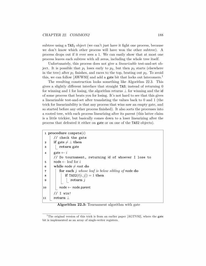
CHAPTER 22. COMMON2 188
subtree using a TAS2 object (we can’t just have it fight one process, becausewe don’t know which other process will have won the other subtree). Aprocess drops out if it ever sees a 1. We can easily show that at most oneprocess leaves each subtree with all zeros, including the whole tree itself.
Unfortunately, this process does not give a linearizable test-and-set ob-ject. It is possible that p1 loses early to p2, but then p3 starts (elsewherein the tree) after p1 finishes, and races to the top, beating out p2. To avoidthis, we can follow [AWW93] and add a gate bit that locks out latecomers.1
The resulting construction looks something like Algorithm 22.3. Thisgives a slightly different interface that straight TAS; instead of returning 0for winning and 1 for losing, the algorithm returns ⊥ for winning and the idof some process that beats you for losing. It’s not hard to see that this givesa linearizable test-and-set after translating the values back to 0 and 1 (thetrick for linearizability is that any process that wins saw an empty gate, andso started before any other process finished). It also sorts the processes intoa rooted tree, with each process linearizing after its parent (this latter claimis a little trickier, but basically comes down to a loser linearizing after theprocess that defeated it either on gate or on one of the TAS2 objects).
1 procedure compete(i)// check the gate
2 if gate 6= ⊥ then3 return gate4 gate← i
// Do tournament, returning id of whoever I lose to5 node← leaf for i6 while node 6= root do7 for each j whose leaf is below sibling of node do8 if TAS2(t[i, j]) = 1 then9 return j
10 node← node.parent// I win!
11 return ⊥
Algorithm 22.3: Tournament algorithm with gate
1The original version of this trick is from an earlier paper [AGTV92], where the gatebit is implemented as an array of single-writer registers.

CHAPTER 22. COMMON2 189
22.3 Single-use swap objectsHere we’ll show how to implement a single-use swap object, where eachprocess is only allowed to execute a single swap operation. The essential ideais to explicitly string the processes into a sequence, where each process learnsthe identity of the process ahead of it. This sequence gives the linearizationorder and allows processes to compute their return values by reading theinput stored by their predecessor.
The algorithm proceeds in asynchronous rounds, with the participantsof each round organized into a tree using the compete procedure from Algo-rithm 22.3. The winner at round k will attempt to thread itself behind someprocess at round k− 1, starting with the process it lost to at that round (ornobody if k = 1). In order for this to work, the round k−1 process must belocked down to round k− 1 (and thread itself behind some other process atround k−1); this is done using a “trap” object implemented with a 2-processswap. If the target process escapes by calling the trap object first, it willleave behind the id of the process it lost to at round k − 1, allowing theround-k winner to try again. If the round-k winner fails to trap anybody, itwill eventually thread itself behind the round-(k − 1) winner, who is stuckat round k − 1.
Only those processes that are ancestors of the process that beat theround-k winner may get trapped in round k − 1; everybody else will escapeand try again in a later round.
Pseudocode for the trap object is given in Algorithm 22.4. There are twooperations. The pass operation is called by the process trying to escape;if it executes first, this process successfully escapes, but leaves behind theidentity of somebody else to try. The block operation locks the target downso that pass fails. The shared data for a trap t consists of a two-processswap object t[i, j] for each process i trying to block a process j. A utilityprocedure passAll is included that calls pass on all potential blockers untilit fails.
It is not hard to see from the code that Algorithm 22.4 has the desiredproperties: if the passer reaches the swap object first, it is not blocked butleaves behind its value v for the passer; while if the blocker reaches theobject first, it obtains no value but successfully blocks the passer.
The full swap construction is given in Algorithm 22.5.This just implements the blocking strategy described before, with the
main swap procedure implementing the round structure and the findValuehelper procedure implementing the walk up the tree.
It’s not hard to see that when all processes finish the protocol, they will

CHAPTER 22. COMMON2 190
1 procedure block(t, j)2 return swap(t[j, i], blocked)
3 procedure pass(t, j, v)4 if swap(t[i, j], v) = blocked then5 return false6 else7 return true
8 procedure passAll(t, v)9 for j ← 1 to n do
10 if ¬pass(t, j, v) then return false11
12 return true
Algorithm 22.4: Trap implementation from [AWW93]
be neatly arranged in a chain with each process except the first obtainingthe value of its predecessor. Slightly less easy to see is that this orderingwill be consistent with the observed execution order, which is necessary forlinearizability. For a proof of linearizability, see the paper.

CHAPTER 22. COMMON2 191
1 procedure swap (v)2 input[i]← v3 for k ← 1 to n do
// find our first target4 t← compete(tournament[k])5 if t = ⊥ then
// I am the round-k winner6 return findValue(k − 1, t′)7 else if ¬passAll(trap[k], t) do
// I did not escape8 return findValue(k, t)9 else
// I escaped, remember who I lost to10 t′ ← t
11 procedure findValue(k, t)12 if k = 0 then13 return ⊥14 else15 repeat16 x← block(trap[k], t)17 if x 6= ⊥ then t← x
18 until x = ⊥19 return input[t]
Algorithm 22.5: Single-use swap from [AWW93]

Chapter 23
Randomized consensus andtest-and-set
We’ve seen that we can’t solve consensus in an asynchronous system withone crash failure [FLP85, LAA87], but that the problem becomes solvableusing failure detectors [CT96]. An alternative that also allows us to solveconsensus is to allow the processes to use randomization, by providing eachprocess with a local coin that can generate random values that are imme-diately visible only to that process. The resulting randomized consensusproblem replaces the termination requirement with probabilistic ter-mination: all processes terminate with probability 1. The agreement andvalidity requirements remain the same.
In this chapter, we will describe how randomization interacts with theadversary, give a bit of history of randomized consensus, and then concen-trate on recent algorithms for randomized consensus and the closely-relatedproblem of randomized test-and-set. Much of the material in this chapter isadapted from notes for a previous course on randomized algorithms [Asp11]and my own recent papers [Asp12b, AE11, Asp12a].
23.1 Role of the adversary in randomized algo-rithms
Because randomized processes are unpredictable, we need to become a littlemore sophisticated in our handling of the adversary. As in previous asyn-chronous protocols, we assume that the adversary has control over timing,which we model by allowing the adversary to choose at each step whichprocess performs the next operation. But now the adversary may do so
192

CHAPTER 23. RANDOMIZED CONSENSUS AND TEST-AND-SET193
based on knowledge of the state of the protocol and its past evolution. Howmuch knowledge we give the adversary affects its power. Several classes ofadversaries have been considered in the literature; ranging from strongestto weakest, we have:
1. An adaptive adversary. This adversary is a function from the stateof the system to the set of processes; it can see everything that hashappened so far (including coin-flips internal to processes that have notyet been revealed to anybody else), but can’t predict the future. It’sknown that an adaptive adversary can force any randomized consensusprotocol to take Θ(n2) total steps [AC08]. The adaptive adversary isalso called a strong adversary following a foundational paper ofAbrahamson [Abr88].
2. An intermediate adversary or weak adversary [Abr88] is onethat limits the adversary’s ability to observe or control the system insome way, without completely eliminating it. For example, a content-oblivious adversary [Cha96] or value-oblivious adversary [Aum97]is restricted from seeing the values contained in registers or pendingwrite operations and from observing the internal states of processesdirectly. A location-oblivious adversary [Asp12b] can distinguishbetween values and the types of pending operations, but can’t discrim-inate between pending operations based one which register they areoperating on. These classes of adversaries are modeled by imposingan equivalence relation on partial executions and insisting that theadversary make the same choice of processes to go next in equivalentsituations. Typically they arise because somebody invented a consen-sus protocol for the oblivious adversary below, and then looked for thenext most powerful adversary that still let the protocol work.Weak adversaries often allow much faster consensus protocols thanadaptive adversaries. Each of the above adversaries permits consensusto be achieved in O(logn) expected individual work using an appropri-ate algorithm. But from a mathematical standpoint, weak adversariesare a bit messy, and once you start combining algorithms designed fordifferent weak adversaries, it’s natural to move all the way down tothe weakest reasonable adversary, the oblivious adversary describedbelow.
3. A oblivious adversary has no ability to observe the system at all;instead, it fixes a sequence of process ids in advance, and at each stepthe next process in the sequence runs.

CHAPTER 23. RANDOMIZED CONSENSUS AND TEST-AND-SET194
We will describe below a protocol that guarantees O(log logn) ex-pected individual work for an oblivious adversary. It is not knownwhether this is optimal; in fact, is is consistent with the best knownlower bound (due to Attiya and Censor [AC08]) that consensus can besolved in O(1) expected individual steps against an oblivious adver-sary.
23.2 HistoryThe use of randomization to solve consensus in an asynchronous systemwith crash failures was proposed by Ben-Or et al.Ben-Or1983 for a message-passing model. Chor, Israeli, and Li [CIL94] gave the first wait-free consen-sus protocol for a shared-memory system, which assumed a particular kindof weak adversary. Abrahamson [Abr88] defined strong and weak adver-saries and gave the first wait-free consensus protocol for a strong adversary;its expected step complexity was Θ
(2n2). After failing to show that expo-
nential time was necessary, Aspnes and Herlihy [AH90a] showed how to doconsensus in O(n4) total work, a value that was soon reduced to O(n2 logn)by Bracha and Rachman [BR91]. This remained the best known bound forthe strong-adversary model until Attiya and Censor [AC08] showed match-ing Θ(n2) upper and lower bounds for the problem; subsequent work [AC09]showed that it was also possible to get an O(n) bound on individual work.
For weak adversaries, the best known upper bound on individual stepcomplexity was O(logn) for a long time [Cha96, Aum97, Asp12b], withan O(n) bound on total step complexity for some models [Asp12b]. Morerecent work has lowered the bound to O(log logn), under the assumption ofan oblivious adversary [Asp12a]. No non-trivial lower bound on expectedindividual step complexity is known, although there is a known lower boundon the distribution of of the individual step complexity [ACH10].
23.3 Reduction to simpler primitivesTo show how to solve consensus using randomization, it helps to split theproblem in two: we will first see how to detect when we’ve achieved agree-ment, and then look at how to achive agreement.

CHAPTER 23. RANDOMIZED CONSENSUS AND TEST-AND-SET195
23.3.1 Adopt-commit objects
Most known randomized consensus protocols have a round-based struc-ture where we alternative between generating and detecting agreement.Gafni [Gaf98] proposed adopt-commit protocols as a tool for detect-ing agreement, and these protocols were later abstracted as adopt-commitobjects [MRRT08, AGGT09]. The version described here is largely takenfrom [AE11], which shows bounds on the complexity of adopt-commit ob-jects.
An adopt-commit object supports a single operation, AdoptCommit (u),where u is an input from a set ofm values. The result of this operation is anoutput of the form (commit, v) or (adopt, v), where the second componentis a value from this set and the first component is a decision bit thatindicates whether the process should decide value v immediately or adopt itas its preferred value in later rounds of the protocol.
The requirements for an adopt-commit object are the usual requirementsof validity and termination, plus:
1. Coherence. If the output of some operation is (commit, v), then everyoutput is either (adopt, v) or (commit, v).
2. Convergence. If all inputs are v, all outputs are (commit, v).
These last two requirement replace the agreement property of consensus.They are also strictly weaker than consensus, which means that a consensusobject (with all its output labeled commit) is also an adopt-commit object.
The reason we like adopt-commit objects is that they allow the simpleconsensus protocol shown in Algorithm 23.1.
1 preference← input2 for r ← 1 . . .∞ do3 (b, preference)← AdoptCommit(AC[r], preference)4 if b = commit then5 return preference6 else7 do something to generate a new preference
Algorithm 23.1: Consensus using adopt-commit
The idea is that the adopt-commit takes care of ensuring that once some-body returns a value (after receiving commit), everybody else who doesn’t

CHAPTER 23. RANDOMIZED CONSENSUS AND TEST-AND-SET196
return adopts the same value (follows from coherence). Conversely, if ev-erybody already has the same value, everybody returns it (follows fromconvergence). The only missing piece is the part where we try to shake allthe processes into agreement. For this we need a separate object called aconciliator.
23.3.2 Conciliators
Conciliators are a weakened version of randomized consensus that replaceagreement with probabilistic agreement: it’s OK if the processes disagreesometimes as long as they agree with constant probability despite interfer-ence by the adversary. An algorithm that satisfies termination, validity, andprobabilistic agreement is called a conciliator.1
The important feature of conciliators is that if we plug a conciliator thatguarantees agreement with probability at least δ into Algorithm 23.1, thenon average we only have to execute the loop 1/δ times before every processagrees. This gives an expected cost equal to 1/δ times the total cost ofAdoptCommit and the conciliator. Typically we will aim for constant δ.
23.4 Implementing an adopt-commit objectWhat’s nice about adopt-commit objects is that they can be implementeddeterministically. Here we’ll give a simple adopt-commit object for twovalues, 0 and 1. Optimal (under certain assumptions) constructions of m-valued adopt-commits can be found in [AE11].
Pseudocode is given in Algorithm 23.2.Structurally, this is pretty similar to a splitter (see §17.4.2, except that
we use values instead of process ids.We now show correctness. Termination and validity are trivial. For
coherence, observe that if I return (commit, v) I must have read a[¬v] = falsebefore any process with ¬v writes a[¬v]; it follows that all such processeswill see proposal 6= ⊥ and return (adopt, v). For convergence, observe thatif all processes have the same input v, they all write it to proposal and allobserve a[¬v] = false, causing them all to return (commit, v).
1Warning: This name has not really caught on in the general theory-of-distributed-computing community, and so far only appears in papers that have a particular researcheras a co-author [Asp12a, AE11, Asp12b]. Unfortunately, there doesn’t seem to be a bettername for the same object that has caught on. So we are stuck with it for now.

CHAPTER 23. RANDOMIZED CONSENSUS AND TEST-AND-SET197
shared data: a[0], a[1], initially false; proposal, initially ⊥1 procedure AdoptCommit(v)2 a[v]← 13 if proposal = ⊥ then4 proposal← v5 else6 v ← proposal
7 if a[¬v] = false then8 return (commit, v)9 else
10 return (adopt, v)
Algorithm 23.2: A 2-valued adopt-commit object
23.5 A one-register conciliator for an oblivious ad-versary
shared data: register r, initially ⊥1 k ← 02 while r = ⊥ do3 with probability 2k
2n do4 write v to r5 else6 do a dummy operation7 k ← k + 18 return r
Algorithm 23.3: Impatient first-mover conciliator from [Asp12b]
Algorithm 23.3 implements a conciliator using a single register; it worksagainst an oblivious adversary.2 This particular construction is taken from [Asp12b],and is based on an earlier algorithm of Chor, Israeli, and Li [CIL94]. Thecost of this algorithm is expected O(n) total work and O(logn) individualwork. It’s not known whether it is possible to improve on this bound.
The basic idea is that processes alternate between reading a register r2Or any adversary dumb enough not to be able to block the write based on how the
coin-flip turned out.

CHAPTER 23. RANDOMIZED CONSENSUS AND TEST-AND-SET198
and (maybe) writing to the register; if a process reads a non-null value fromthe register, it returns it. Any other process that reads the same non-nullvalue will agree with the first process; the only way that this can’t happenis if some process writes a different value to the register before it notices thefirst write.
The random choice of whether to write the register or not avoids thisproblem. The idea is that even though the adversary can schedule a writeat a particular time, because it’s oblivious, it won’t be able to tell if theprocess wrote (or was about to write) or did a no-op instead.
The basic version of this algorithm, due to Chor, Israeli, and Li [CIL94],uses a fixed 1
2n probability of writing to the register. So once some processwrites to the register, the chance that any of the remaining n− 1 processeswrite to it before noticing that it’s non-null is at most n−1
2n < 1/2. It’s alsonot hard to see that this algorithm uses O(n) total operations, although itmay be that one single process running by itself has to go through the loop2n times before it finally writes the register and escapes.
Using increasing probabilities avoids this problem, because any processthat executes the main loop dlgne + 1 times will write the register. Thisestablishes the O(logn) per-process bound on operations. At the same time,an O(n) bound on total operations still holds, since each write has at leasta 1
2n chance of succeeding. The price we pay for the improvement is thatwe increase the chance that an initial value written to the register getsoverwritten by some high-probability write. But the intuition is that theprobabilities can’t grow too much, because the probability that I write onmy next write is close to the sum of the probabilities that I wrote on myprevious writes—suggesting that if I have a high probability of writing nexttime, I should have done a write already.
Formalizing this intuition requires a little bit of work. Fix the schedule,and let pi be the probability that the i-th write operation in this schedulesucceeds. Let t be the least value for which
∑ti=1 pi ≥ 1/4. We’re going to
argue that with constant probability one of the first t writes succeeds, andthat the next n− 1 writes by different processes all fail.
The probability that none of the first t writes succeed ist∏i=1
(1− pi) ≤t∏i=1
e−pi
= exp(
t∑i=1
pi
)≤ e−1/4.

CHAPTER 23. RANDOMIZED CONSENSUS AND TEST-AND-SET199
Now observe that if some process q writes at or before the t-th write,then any process with a pending write either did no writes previously, or itslast write was among the first t − 1 writes, whose probabilities sum to lessthan 1/4. In the first case, the process has a 1
2n chance of writing on itsnext attempt. In the second, it has a
∑i∈Sq
pi + 12n chance of writing on its
next attempt, where Sq is the set of indices in 1 . . . t − 1 where q attemptsto write.
Summing up these probabilities over all processes gives a total of n−12n +∑
q
∑i∈Sq
pi ≤ 1/2+1/4 = 3/4. So with probabililty at least e−1/4(1−3/4) =e−1/4/4, we get agreement.
23.6 SiftersA faster conciliator can be obtained using a sifter, which is a mechanism forrapidly discarding processes using randomization [AA11] while keeping atleast one process around. The idea of a sifter is to have each process eitherwrite a register (with low probability) or read it (with high probability); allwriters and all readers that see ⊥ continue to the next stage of the protocol,while all readers who see a non-null value drop out. An appropriately-tuned sifter will reduce n processes to at most 2
√n processes on average; by
iterating this mechanism, the expected number of remaining processes canbe reduced to 1 + ε after O(log logn+ log(1/ε)) phases.
As with previous implementations of test-and-set (see Algorithm 22.3),it’s often helpful to have a sifter return not only that a process lost but whichprocess it lost to. This gives the implementation shown in Algorithm 23.4.
1 procedure sifter(p, r)2 with probability p do3 r ← id4 return ⊥5 else6 return r
Algorithm 23.4: A sifter
To use a sifter effectively, p should be tuned to match the number ofprocesses that are likely to use it. This is because of the following lemma:

CHAPTER 23. RANDOMIZED CONSENSUS AND TEST-AND-SET200
Lemma 23.6.1. Fix p, and let X processes executed a sifter with parameterp. Let Y be the number of processes for which the sifter returns ⊥. Then
E [X | Y ] ≤ pX + 1p. (23.6.1)
Proof. In order to return ⊥, a process must either (a) write to r, whichoccurs with probability p, or (b) read r before any other process writes toit. The expected number of writers, conditioned on X, is exactly pX. Theexpected number of readers before the first write has a geometric distributiontruncated by X. Removing the truncation gives exactly 1
p expected readers,which is an upper bound on the correct value.
For n initial processes, the choice of p that minimizes the bound in(23.6.1) is 1√
n, giving at most 2
√n expected survivors. Iterating this process
with optimal p at each step gives a sequence of at most n, 2√n, 2
√2√n,
etc., expected survivors after each sifter. The twos are a little annoying, buta straightforward induction bounds the expected survivors after i rounds by4 · n2−i . In particular, we get at most 8 expected survivors after dlg lgnerounds.
At this point it makes sense to switch to a fixed p and a different anal-ysis. For p = 1/2, the first process to access r always survives, and eachsubsequent process survives with probability at most 3/4 (because it leavesif the first process writes and it reads). So the number of “excess” processesdrops as (3/4)i, and an additional
⌈log4/3(7/ε)
⌉rounds are enough to reduce
the expected number of survivors from 1 + 7 to 1 + ε for any fixed ε.3It follows that
Theorem 23.6.2. An initial set of n processes can be reduced to 1 withprobability at least 1− ε using O(log logn+ log(1/ε)) rounds of sifters.
Proof. LetX be the number of survivors after dlg lgne+⌈log4/3(7/ε)
⌉rounds
of sifters, with probabilities tuned as described above. We’ve shown thatE [X] ≤ 1 + ε, so E [X − 1] ≤ ε. Since X − 1 ≥ 0, from Markov’s inequalitywe have Pr [X ≥ 2] = Pr [X − 1 ≥ 1] ≤ E [X − 1] /1 ≤ ε.
3This argument essentially follows the proof of [Asp12a, Theorem 2], which, becauseof neglecting to subtract off a 1 at one point, ends up with 8/ε instead of 7/ε.

CHAPTER 23. RANDOMIZED CONSENSUS AND TEST-AND-SET201
23.6.1 Test-and-set using sifters
Sifters were initially designed to be used for test-and-set. For this purpose,we treat a return value of ⊥ as “keep going” and anything else as “leavewith value 1.” Using O(log logn) rounds of sifters, we can get down to oneprocess that hasn’t left with probability at least 1 − log−c n for any fixedconstant c. We then need a fall-back TAS to handle the log−c n chance thatwe get more than one such survivor.
Alistarh and Aspnes [AA11] used the RatRace algorithm of Alistarh etal. [AAG+10] for this purpose. This is an adaptive randomized test-and-setbuilt from splitters and two-process consensus objects that runs in O(log k)expected time, where k is the number of processes that access the test-and-set; a sketch of this algorithm is given in §24.5.2. If we want to avoid appeal-ing to this algorithm, a somewhat simpler approach is to use an approachsimilar to the Lamport’s fast-path mutual exclusion algorithm (described in§17.4.2): any process that survives the splitters tries to rush to a two-processTAS at the top of a tree of two-processes TASes by winning a splitter, andif it doesn’t win the splitter, it enters at a leaf and pays O(logn) expectedsteps. By setting ε = 1/ logn, the overall expected cost of this final stage isO(1).
This algorithm does not guarantee linearizability. I might lose a sifterearly on only to have a later process win all the sifters (say, by writing toeach one) and return 0. A gate bit as in Algorithm 22.3 solves this problem.The full code is given in Algorithm 23.5.
23.6.2 Consensus using sifters
With some trickery, the sifter mechanism can be adapted to solve consensus,still in O(log logn) expected individual work [Asp12a]. The main difficultyis that a process can no longer drop out as soon as it knows that it lost:it still needs to figure out who won, and possible help that winner over thefinish line.
The basic idea is that when a process p loses a sifter to some other processq, p will act like a clone of q from that point on. In order to make this work,each process writes down at the start of the protocol all of the coin-flips itintends to use to decide whether to read or write at each round of sifting.Together with its input, these coin-flips make up the process’s persona.In analyzing the progress of the sifter, we count surviving personae (withmultiple copies of the same persona counting as one) instead of survivingprocesses.

CHAPTER 23. RANDOMIZED CONSENSUS AND TEST-AND-SET202
1 if gate 6= ⊥ then2 return 13 else4 gate← myId5 for i← 1 . . . dlog logne+
⌈log4/3(7 logn)
⌉do
6 with probability min(1/2, 21−2−i+1
)do
7 ri ← myId8 else9 w ← ri
10 if w 6= ⊥ then11 return 1
12 if splitter() = stop then13 return 014 else15 return AWWTAS()
Algorithm 23.5: Test-and-set in O(log logn) expected time
Pseudocode for this algorithm is given in Algorithm 23.6. Note that theloop body is essentially the same as the code in Algorithm 23.4, except thatthe random choice is replaced by a lookup in persona.chooseWrite.
To show that this works, we need to argue that having multiple copiesof a persona around doesn’t change the behavior of the sifter. In eachround, we will call the first process with a given persona p to access rithe representative of p, and argue that a persona survives round i inthis algorithm precisely when its representative would survive round i ina corresponding test-and-set sifter with the schedule restricted only to therepresentatives.
There are three cases:
1. The representative of p writes. Then at least one copy of p survives.
2. The representative of p reads a null value. Again at least one copy ofp survives.
3. The representative of p reads a non-null value. Then no copy of psurvives: all subsequent reads by processes carrying p also read a non-null value and discard p, and since no process with p writes, no otherprocess adopts p.

CHAPTER 23. RANDOMIZED CONSENSUS AND TEST-AND-SET203
1 procedure conciliator(input)2 Let R = dlog logne+
⌈log4/3(7/ε)
⌉3 Let chooseWrite be a vector of R independent random Boolean
variables with Pr[chooseWrite[i] = 1] = pi, wherepi = 21−2−i+1(n)−2−i for i ≤ dlog logne and pi = 1/2 for larger i.
4 persona← 〈input, chooseWrite,myId〉5 for i← 1 . . . R do6 if persona.chooseWrite[i] = 1 then7 ri ← persona8 else9 v ← ri
10 if v 6= ⊥ then11 persona← v
12 return persona.input
Algorithm 23.6: Sifting conciliator (from [Asp12a])
From the preceding analysis for test-and-set, we have that afterO(log logn+log 1/ε) rounds with appropriate probabilities of writing, at most 1+ε valuessurvive on average. This gives a probability of at most ε of disagreement. Byalternating these conciliators with adopt-commit objects, we get agreementin O(log logn + logm/ log logm) expected time, where m is the number ofpossible input values.
I don’t think the O(log logn) part of this expression is optimal, but Idon’t know how to do better.
23.7 O(log∗ n) Randomized test-and-setA more sophisticated sifter due to Giakkoupis and Woelfel [GW12a] removesall but O(logn) processes, on average, using two operations for each pro-cess. Iterating this sifter reduces the expected survivors to O(1) in O(log∗ n)rounds. A particularly nice feature of the Giakkoupis-Woelfel algorithm isthat (if you don’t care about space) it doesn’t have any parameters thatrequire tuning to n: this means that exactly the same structure can be usedin each round. An unfortunate feature is that it’s not possible to guaran-tee that every process that leaves learns the identity of a process that stays:this means that it can’t adapted into a consensus protocol using the persona

CHAPTER 23. RANDOMIZED CONSENSUS AND TEST-AND-SET204
trick described in §23.6.2.Pseudocode is given in Algorithm 23.7. In this simplified version, we
assume an infinitely long array A[1 . . . ], so that we don’t need to worryabout n. Truncating the array at logn also works, but the analysis requireshandling the last position as a special case, which I am too lazy to do here.
1 Choose r ∈ Z+ such that Pr [r = i] = 2−i2 A[r]← 13 if A[r + 1] = 0 then4 stay5 else6 leave
Algorithm 23.7: Giakkoupis-Woelfel sifter [GW12a]
Lemma 23.7.1. In any execution of Algorithm 23.7 with an oblivious ad-versary and n processes, at least one process stays, and the expected numberof processes that stay is O(logn).
Proof. For the first part, observe that any process that picks the largestvalue of r among all processes will survive; since the number of processes isfinite, there is at least one such survivor.
For the second part, let Xi be the number of survivors with r = i. ThenE [Xi] is bounded by n · 2−i, since no process survives with r = i withoutfirst choosing r = i. But we can also argue that E [Xi] ≤ 3 for any value ofn, by considering the sequence of write operations in the execution.
Because the adversary is oblivious, the location of these writes is uncor-related with their ordering. If we assume that the adversary is trying tomaximize the number of survivors, its best strategy is to allow each processto read immediately after writing, as delaying this read can only increase theprobability that A[r + 1] is nonzero. So in computing Xi, we are countingthe number of writes to A[i] before the first write to A[i + 1]. Let’s ignoreall writes to other registers; then the j-th write to either of A[i] or A[i+ 1]has a conditional probability of 2/3 of landing on A[i] and 1/3 on A[i+ 1].We are thus looking at a geometric distribution with parameter 1/3, whichhas expectation 3.

CHAPTER 23. RANDOMIZED CONSENSUS AND TEST-AND-SET205
Combining these two bounds gives E [Xi] ≤ min(3, 2−i). So then
E [survivors] ≤∞∑i=1
min(3, n · 2−i)
= 3 lgn+O(1),
because once n · 2−i drops below 3, the remaining terms form a geometricseries.
Like square root, logarithm is concave, so Jensen’s inequality applies hereas well. So O(log∗ n) rounds of Algorithm 23.7 reduces us to an expectedconstant number of survivors, which can then be fed to RatRace.
With an adaptive adversary, all of the sifter-based test-and-sets failbadly: in this particular case, an adaptive adversary can sort the processesin order of increasing write location so that every process survives. The bestknown n-process test-and-set for an adaptive adversary is still a tree of 2-process randomized test-and-sets, as in the Afek et al. [AWW93] algorithmdescribed in §22.2. Whether O(logn) expected steps is in fact necessaryis still open (as is the exact complexity of test-and-set with an obliviousadversary).
23.8 Space boundsA classic result of Fich, Herlihy, and Shavit [FHS98] shows that Ω(
√n) reg-
isters are needed to solve consensus even under the very weak requirement ofnondeterministic solo termination, which says that for every reachableconfiguration and every process p, there exists some continuation of the exe-cution in which the protocol terminates with only p running. The best knownupper bound is the trivial n—one single-writer register per process—sinceany multi-writer register algorithm can be translated into a single-writer al-gorithm and (assuming wide enough registers) multiple registers of a singleprocess can be combined into one.
There has been very little progress in closing the gap between thesetwo bounds since the original conference version of the FHS paper from1993, although very recently, Giakkoupis et al. [GHHW13] have shown asurprising O(
√n)-space algorithm for the closely related problem of leader
election, which is basically test-and-set without guaranteeing linearizability.The main difference between leader election and consensus is that in consen-sus every process learns the identity of the winner, instead of just whether

CHAPTER 23. RANDOMIZED CONSENSUS AND TEST-AND-SET206
it personally won or lost. It is not clear whether the techniques used for thisproblem could carry across to consensus.

Chapter 24
Renaming
We will start by following the presentation in [AW04, §16.3]. This mostly de-scribes results of the original paper of Attiya et al. [ABND+90] that definedthe renaming problem and gave a solution for message-passing; however, it’snow more common to treat renaming in the context of shared-memory, sowe will follow Attiya and Welch’s translation of these results to a shared-memory setting.
24.1 RenamingIn the renaming problem, we have n processes, each starts with a namefrom some huge namespace, and we’d like to assign them each unique namesfrom a much smaller namespace. The main application is allowing us to runalgorithms that assume that the processes are given contiguous numbers,e.g. the various collect or atomic snapshot algorithms in which each processis assigned a unique register and we have to read all of the registers. Withrenaming, instead of reading a huge pile of registers in order to find the fewthat are actually used, we can map the processes down to a much smallerset.
Formally, we have a decision problem where each process has input xi(its original name) and output yi, with the requirements:
Termination Every nonfaulty process eventually decides.
Uniqueness If pi 6= pj , then yi 6= yj .
Anonymity The code executed by any process depends only on its inputxi: for any execution of processes p1 . . . pn with inputs x1 . . . xn, and
207

CHAPTER 24. RENAMING 208
any permutation π of [1 . . . n], there is a corresponding execution ofprocesses pπ(1) . . . pπ(n) with inputs x1 . . . xn in which pπ(i) performsexactly the same operations as pi and obtains the same output yi.
The last condition is like non-triviality for consensus: it excludes algo-rithms where pi just returns i in all executions. Typically we do not haveto do much to prove anonymity other than observing that all processes arerunning the same code.
We will be considering renaming in a shared-memory system, where weonly have atomic registers to work with.
24.2 PerformanceConventions on counting processes:
• N = number of possible original names.
• n = maximum number of processes.
• k = number of processes that actually execute the algorithm.
Ideally, we’d like any performance measures we get to depend on k aloneif possible (giving an adaptive algorithm). Next best would be somethingpolynomial in n and k. Anything involving N is bad.
We’d also like to minimize the size of the output namespace. How wellwe can do this depends on what assumptions we make. For deterministicalgorithms using only read-write registers, a lower bound due to Herlihy andShavit [HS99] shows that we can’t get fewer than 2n− 1 names for generaln.1 Our target thus will be exactly 2n−1 output names if possible, or 2k−1if we are trying to be adaptive. For randomized algorithm, it is possible tosolve strong or tight renaming, where the size of the namespace is exactlyk; we’ll see how to do this in §24.5.
A small note on bounds: There is a lot of variation in the literature onhow bounds on the size of the output namespace are stated. The originalHerlihy-Shavit lower bound [HS99] says that there is no general renamingalgorithm that uses 2n names for n + 1 processes; in other words, any n-process algorithm uses at least 2n − 1 names. Many subsequent papers
1This lower bound was further refined by Castañeda and Rajsbaum [CR08], who showthat 2n − 2 (but no less!) is possible for certain special values of n; all of these lowerbounds make extensive use of combinatorial topology, so we won’t try to present themhere.

CHAPTER 24. RENAMING 209
discussing lower bounds on the namespace follow the approach of Herlihy andShavit and quote lower bounds that are generally 2 higher than the minimumnumber of names needed for n processes. This requires a certain amount oftranslation when comparing these lower bounds with upper bounds, whichuse the more natural convention.
24.3 Order-preserving renamingBefore we jump into upper bounds, let’s do an easy lower bound from theAttiya et al. paper [ABND+90]. This bound works on a variant of renamingcalled order-preserving renaming, where we require that yi < yj when-ever xi < xj . Unfortunately, this requires a very large output namespace:with t failures, any asynchronous algorithm for order-preserving renamingrequires 2t(n− t+ 1)− 1 possible output names. This lower bound appliesregardless of the model, as long as some processes may start after otherprocesses have already been assigned names.
For the wait-free case, we have t = n − 1, and the bound becomes just2n−1. This is a simpler case than the general t-failure case, but the essentialidea is the same: if I’ve only seen a few of the processes, I need to leave roomfor the others.
Theorem 24.3.1. There is no order-preserving renaming algorithm for nprocesses using fewer than 2n − 1 names.
Proof. By induction on n. For n = 1, we use 21 − 1 = 1 names; this is thebase case. For larger n, suppose we use m names, and consider an executionin which one process pn runs to completion first. This consumes one nameyn and leaves k names less than yn and m−k−1 names greater than yn. Bysetting all the inputs xi for i < n either less than xn or greater than xn, wecan force the remaining processes to choose from the remaining k orm−k−1names. Applying the induction hypothesis, this gives k ≥ 2n−1 − 1 andm−k−1 ≥ 2n−1−1, som = k+(m−k−1)+1 ≥ 2(2n−1−1)+1 = 2n−1.
24.4 Deterministic renamingIn deterministic renaming, we can’t use randomization, and may or maynot have any primitives stronger than atomic registers. With just atomicregisters, we can only solve loose renaming; with test-and-set, we can solvetight renaming. In this section, we describe some basic algorithms for de-terministic renaming.

CHAPTER 24. RENAMING 210
24.4.1 Wait-free renaming with 2n− 1 names
Here we use Algorithm 55 from [AW04], which is an adaptation to sharedmemory of the message-passing renaming algorithm of [ABND+90]. Oneodd feature of the algorithm is that, as written, it is not anonymous: pro-cesses communicate using an atomic snapshot object and use their processids to select which component of the snapshot array to write to. But if wethink of the process ids used in the algorithm as the inputs xi rather thanthe actual process ids i, then everything works. The version given in Algo-rithm 24.1 makes this substitution explicit, by treating the original name ias the input.
1 procedure getName()2 s← 13 while true do4 a[i]← s5 view← snapshot(a)6 if view[j] = s for some j then7 r ← |j : view[j] 6= ⊥ ∧ j ≤ i|8 s← r-th positive integer not in
view[j] : j 6= i ∧ view[j] = ⊥9 else
10 return s
Algorithm 24.1: Wait-free deterministic renaming
The array a holds proposed names for each process (indexed by theoriginal names), or ⊥ for processes that have not proposed a name yet. If aprocess proposes a name and finds that no other process has proposed thesame name, it takes it; otherwise it chooses a new name by first computingits rank r among the active processes and then choosing the r-th smallestname that hasn’t been proposed by another process. Because the rank is atmost n and there are at most n− 1 names proposed by the other processes,this always gives proposed names in the range [1 . . . 2n− 1]. But it remainsto show that the algorithm satisfies uniqueness and termination.
For uniqueness, consider two process with original names i and j. Sup-pose that i and j both decide on s. Then i sees a view in which a[i] = s anda[j] 6= s, after which it no longer updates a[i]. Similarly, j sees a view inwhich a[j] = s and a[i] 6= s, after which it no longer updates a[j]. If i’s viewis obtained first, then j can’t see a[i] 6= s, but the same holds if j’s view is

CHAPTER 24. RENAMING 211
obtained first. So in either case we get a contradiction, proving uniqueness.Termination is a bit trickier. Here we argue that no process can run
forever without picking a name, by showing that if we have a set of processesthat are doing this, the one with smallest original name eventually picks aname. More formally, call a process trying if it runs for infinitely many stepswithout choosing a name. Then in any execution with at least one tryingprocess, eventually we reach a configuration where all processes have eitherfinished or are trying. In some subsequent configuration, all the processeshave written to the a array at least once; from this point on, the set of non-null positions in a—and thus the rank each process computes for itself—isstable.
Starting from some such stable configuration, look at the trying processi with the smallest original name, and suppose it has rank r. Let F =z1 < z2 . . . be the set of “free names” that are not proposed in a by any ofthe finished processes. Observe that no trying process j 6= i ever proposesa name in z1 . . . zr, because any such process has rank greater than r.This leaves zr open for i to claim, provided the other names in z1 . . . zreventually become free. But this will happen, because only trying processesmay have proposed these names (early on in the execution, when the finishedprocesses hadn’t finished yet), and the trying processes eventually proposenew names that are not in this range. So eventually process i proposes zr,sees no conflict, and finishes, contradicting the assumption that it is trying.
Note that we haven’t proved any complexity bounds on this algorithm atall, but we know that the snapshot alone takes at least Ω(N) time and space.Brodksy et al. [BEW11] cite a paper of Bar-Noy and Dolev [BND89] as givinga shared-memory version of [ABND+90] with complexity O(n ·4n); they alsogive algorithms and pointers to algorithms with much better complexity.
24.4.2 Long-lived renaming
In long-lived renaming a process can release a name for later use by otherprocesses (or the same process, if it happens to run choose-name again). Nowthe bound on the number of names needed is 2k−1, where k is the maximumnumber of concurrently active processes. Algorithm 24.1 can be convertedto a long-lived renaming algorithm by adding the releaseName proceduregiven in Algorithm 24.2. This just erases the process’s proposed name, sothat some other process can claim it.
Here the termination requirement is weakened slightly, to say that someprocess always makes progress in getName. It may be, however, that thereis some process that never successfully obtains a name, because it keeps

CHAPTER 24. RENAMING 212
1 procedure releaseName()2 a[i]← ⊥
Algorithm 24.2: Releasing a name
getting stepped on by other processes zipping in and out of getName andreleaseName.
24.4.3 Renaming without snapshots
Moir and Anderson [MA95] give a renaming protocol that is somewhat easierto understand and doesn’t require taking snapshots over huge arrays. Adownside is that the basic version requires k(k + 1)/2 names to handle kactive processes.
24.4.3.1 Splitters
The Moir-Anderson renaming protocol uses a network of splitters, whichwe last saw providing a fast path for mutual exclusion in §17.4.2. Eachsplitter is a widget, built from a pair of atomic registers, that assigns toeach processes that arrives at it the value right, down, or stop. As discussedpreviously, the useful properties of splitters are that if at least one processarrives at a splitter, then (a) at least one process returns right or stop; and(b) at least one process returns down or stop; (c) at most one process returnsstop; and (d) any process that runs by itself returns stop.
We proved the last two properties in §17.4.2; we’ll prove the first twohere. Another way of describing these properties is that of all the processesthat arrive at a splitter, some process doesn’t go down and some processdoesn’t go right. By arranging splitters in a grid, this property guaranteesthat every row or column that gets at least one process gets to keep it—which means that with k processes, no process reaches row k+ 1 or columnk + 1.
Algorithm 24.3 gives the implementation of a splitter (it’s identical toAlgorithm 17.5, but it will be convenient to have another copy here).
Lemma 24.4.1. If at least one process completes the splitter, at least oneprocess returns stop or right.
Proof. Suppose no process returns right; then every process sees open indoor, which means that every process writes its id to race before any process

CHAPTER 24. RENAMING 213
shared data:1 atomic register race, big enough to hold an id, initially ⊥2 atomic register door, big enough to hold a bit, initially open3 procedure splitter(id)4 race← id5 if door = closed then6 return right7 door← closed8 if race = id then9 return stop
10 else11 return down
Algorithm 24.3: Implementation of a splitter
closes the door. Some process writes its id last: this process will see its ownid in race and return stop.
Lemma 24.4.2. If at least one process completes the splitter, at least oneprocess returns stop or down.
Proof. First observe that if no process ever writes to door, then no processcompletes the splitter, because the only way a process can finish the splitterwithout writing to door is if it sees closed when it reads door (which musthave been written by some other process). So if at least one process finishes,at least one process writes to door. Let p be any such process. From thecode, having written door, it has already passed up the chance to returnright; thus it either returns stop or down.
24.4.3.2 Splitters in a grid
Now build anm-by-m triangular grid of splitters, arranged as rows 0 . . .m−1and columns 0 . . .m − 1, where a splitter appears in each position (r, c)with r + c ≤ m − 1 (see Figure 24.1 for an example; this figure is takenfrom [Asp10]). Assign a distinct name to each of the
(m2)splitters in this
grid. To obtain a name, a process starts at (r, c) = (0, 0), and repeatedlyexecutes the splitter at its current position (r, c). If the splitter returns right,it moves to (r, c + 1); if down, it moves to (r + 1, c); if stop, it stops, andreturns the name of its current splitter. This gives each name to at most

CHAPTER 24. RENAMING 214
Figure 24.1: A 6× 6 Moir-Anderson grid
one process (by Lemma 17.4.3); we also have to show that if at most mprocesses enter the grid, every process stops at some splitter.
The argument for this is simple. Suppose some process p leaves thegrid on one of the 2m output wires. Look at the path it takes to get there(see Figure 24.2, also taken from [Asp10]). Each splitter on this path musthandle at least two processes (or p would have stopped at that splitter, byLemma 17.4.4). So some other process leaves on the other output wire, eitherright or down. If we draw a path from each of these wires that continues rightor down to the end of the grid, then along each of these m disjoint pathseither some splitter stops a process, or some process reaches a final outputwire, each of which is at a distinct splitter. But this gives m processes inaddition to p, for a total of m+ 1 processes. It follows that:
Theorem 24.4.3. An m ×m Moir-Anderson grid solves renaming for upto m processes.
The time complexity of the algorithm is O(m): Each process spends atmost 4 operations on each splitter, and no process goes through more than2m splitters. In general, any splitter network will take at least n steps tostop n processes, because the adversary can run them all together in a hordethat drops only one process at each splitter.
If we don’t know k in advance, we can still guarantee names of size O(k2)by carefully arranging them so that each k-by-k subgrid contains the first
(k2)
names. This gives an adaptive renaming algorithm (although the namespace

CHAPTER 24. RENAMING 215
Figure 24.2: Path taken by a single process through a 6× 6 Moir-Andersongrid (heavy path), and the 6 disjoint paths it spawns (dashed paths).
size is pretty high). We still have to choose our grid to be large enough forthe largest k we might actually encounter; the resulting space complexity isO(n2).
With a slightly more clever arrangement of the splitters, it is possible toreduce the space complexity to O(n3/2) [Asp10]. Whether further reductionsare possible is an open problem. Note however that linear time complexitymakes splitter networks uncompetitive with much faster randomized algo-rithms (as we’ll see in §24.5), so this may not be a very important openproblem.
24.4.4 Getting to 2n− 1 names in polynomial space
From before, we have an algorithm that will get 2n − 1 names for n pro-cesses out of N possible processes when run using O(N) space (for theenormous snapshots). To turn this into a bounded-space algorithm, runMoir-Anderson first to get down to Θ(k2) names, then run the previousalgorithm (in Θ(n2) space) using these new names as the original names.
Since we didn’t prove anything about time complexity of the humongous-snapshot algorithm, we can’t say much about the time complexity of thiscombined one. Moir and Anderson suggest instead using an O(Nk2) algo-rithm of Borowsky and Gafni to get O(k4) time for the combined algorithm.
This is close to the best known: a later paper by Afek and Merritt [AM99]

CHAPTER 24. RENAMING 216
holds the current record for deterministic adaptive renaming into 2k − 1names at O(k2) individual steps. On the lower bound side, it is known thatΩ(k) is a lower bound on the individual steps of any renaming protocol witha polynomial output namespace [AAGG11].
24.4.5 Renaming with test-and-set
Moir and Anderson give a simple renaming algorithm based on test-and-setthat is strong (k processes are assigned exactly the names 1 . . . k), adaptive(the time complexity to acquire a name is O(k)), and long-lived, whichmeans that a process can release its name and the name will be available toprocesses that arrive later. In fact, the resulting algorithm gives long-livedstrong renaming, meaning that the set of names in use will always be nolarger than the set of processes that have started to acquire a name and notyet finished releasing one; this is a little stronger than just saying that thealgorithm is strong and that it is long-lived separately.
The algorithm is simple: we have a line of test-and-set bits T [1] . . . T [n].To acquire a name, a process starts at T [1] and attempts to win each test-and-set until it succeeds; whichever T [i] it wins gives it name i. To releasea name, a process releases the test-and-set.
Without the releases, the same mechanism gives fetch-and-increment [AWW93].Fetch-and-increment by itself solves tight renaming (although not long-livedrenaming, since there is no way to release a name).
24.5 Randomized renamingWith randomization, we can beat both the 2k−1 lower bound on the size ofthe output namespace from [HS99] and the Ω(k) lower bound on individualwork from [AAGG11], achieving strong renaming with O(log k) expectedindividual work [AACH+11].
The basic idea is that we can use randomization for load balancing,where we avoid the problem of having an army of processes marching to-gether with only a few peeling off at a time (as in splitter networks) byhaving the processes split up based on random choices. For example, if eachprocess generates a random name consisting of 2 dlgne bits, then it is rea-sonably likely that every process gets a unique name in a namespace of sizeO(n2) (we can’t hope for less than O(n2) because of the birthday para-dox). But we want all processes to be guaranteed to have unique names, sowe need some more machinery.

CHAPTER 24. RENAMING 217
We also need the processes to have initial names; if they don’t, thereis always some nonzero probability that two identical processes will fliptheir coins in exactly the same way and end up with the same name.This observation was formalized by Buhrman, Panconesi, Silvestri, andVitányi [BPSV06].
24.5.1 Randomized splitters
Attiya, Kuhn, Plaxton, Wattenhofer, and Wattenhofer [AKP+06] suggestedthe use of randomized splitters in the context of another problem (adap-tive collect) that is closely related to renaming.
A randomized splitter is just like a regular splitter, except that if aprocess doesn’t stop it flips a coin to decide whether to go right or down.Randomized splitters are nice because they usually split better than de-terministic splitters: if k processes reach a randomized splitter, with highprobability no more than k/2+O(
√k log k) will leave on either output wire.
It’s not hard to show that a binary tree of these things of depth 2 dlgnestops all but a constant expected number of processes on average;2 processesthat don’t stop can be dropped into a backup renaming algorithm (Moir-Anderson, for example) only a constant increase in expected individual work.
Furthermore, the binary tree of randomized splitters is adaptive; if onlyk processes show up, we only need O(log k) levels levels on average to splitthem up. This gives renaming into a namespace with expected size O(k2)in O(log k) expected individual steps.
24.5.2 Randomized test-and-set plus sampling
Subsequent work by Alistarh et al. [AAG+10] showed how some of the sameideas could be used to get strong renaming, where the output namespace hassize exactly n (note this is not adaptive; another result in the same papergives adaptive renaming, but it’s not strong). There are two pieces to thisresult: an implementation of randomized test-and-set called RatRace, anda sampling procedure for getting names called ReShuffle.
The RatRace protocol implements a randomized test-and-set withO(log k)expected individual work. The essential idea is to use a tree of randomizedsplitters to assign names, then have processes walk back up the same tree
2The proof is to consider the expected number of pairs of processes that flip their coinsthe same way for all 2 dlgne steps. This is at most
(n2
)n−2 < 1/2, so on average at most 1
process escapes the tree, giving (by symmetry) at most a 1/n chance that any particularprocess escapes. Making the tree deeper can give any polynomial fraction of escapeeswhile still keeping O(logn) layers.

CHAPTER 24. RENAMING 218
attempting to win a 3-process randomized test-and-set at each node (thereare 3 processes, because in addition to the winners of each subtree, we mayalso have a process that stopped on that node in the renaming step); thistest-and-set is just a very small binary tree of 2-process test-and-sets im-plemented using the algorithm of Tromp and Vitányi [TV02]. A gate bit isadded at the top as in the test-and-set protocol of Afek et al. [AGTV92] toget linearizability.
Once we have test-and-set, we could get strong renaming using a lineararray of test-and-sets as suggested by Moir and Anderson [MA95], but it’smore efficient to use the randomization to spread the processes out. Inthe ReShuffle protocol, each process chooses a name in the range [1 . . . n]uniformly at random, and attempts to win a test-and-set guarding thatname. If it doesn’t work, it tries again. Alistarh et al. show that this methodproduces unique names for everybody in O(n log4 n) total steps with highprobability. The individual step complexity of this algorithm, however, isnot very good: there is likely to be some unlucky process that needs Ω(n)probes (at an expected cost of Θ(logn) steps each) to find an empty slot.
24.5.3 Renaming with sorting networks
A later paper by Alistarh et al. [AACH+11] reduces the cost of renamingstill further, getting O(log k) expected individual step complexity for acquir-ing a name. The resulting algorithm is both adaptive and strong: with kprocesses, only names 1 through k are used. We’ll describe the non-adaptiveversion here.
The basic idea is to build a sorting network out of test-and-sets; the re-sulting structure, called a renaming network, routes each process througha sequence of test-and-sets to a unique output wire. Unlike a splitter net-work, a renaming network uses the stronger properties of test-and-set toguarantee that (once the dust settles) only the lowest-numbered output wiresare chosen; this gives strong renaming.
24.5.3.1 Sorting networks
A sorting network is a kind of parallel sorting algorithm that proceeds insynchronous rounds, where in each round the elements of an array at certainfixed positions are paired off and swapped if they are out of order. Thedifference between a sorting network and a standard comparison-based sortis that the choice of which positions to compare at each step is static, anddoesn’t depend on the outcome of previous comparisons; also, the only effect

CHAPTER 24. RENAMING 219
Figure 24.3: A sorting network
of a comparison is possibly swapping the two values that were compared.Sorting networks are drawn as in Figure 24.3. Each horizontal line or
wire corresponds to a position in the array. The vertical lines are com-parators that compare two values coming in from the left and swap thelarger value to the bottom. A network of comparators is a sorting networkif the sequences of output values is always sorted no matter what the orderof values on the inputs is.
The depth of a sorting network is the maximum number of comparatorson any path from an input to an output. The width is the number of wires;equivalently, the number of values the network can sort. The sorting networkin Figure 24.3 has depth 3 and width 4.
Explicit constructions of sorting networks with width n and depthO(log2 n)are known [Bat68]. It is also known that sorting networks with depthO(logn) exist [AKS83], but no explicit construction of such a network isknown.
24.5.3.2 Renaming networks
To turn a sorting network into a renaming network, we replace the compara-tors with test-and-set bits, and allow processes to walk through the networkasynchronously. This is similar to an earlier mechanism called a countingnetwork [AHS94], which used certain special classes of sorting networks ascounters, but here any sorting network works.
Each process starts on a separate input wire, and we maintain the in-

CHAPTER 24. RENAMING 220
variant that at most one process ever traverses a wire. It follows that eachtest-and-set bit is only used by two processes. The first process to reach thetest-and-set bit is sent out the lower output, while the second is sent out theupper output. If we imagine each process that participates in the protocolas a one and each process that doesn’t as a zero, the test-and-set bit actsas a comparator: if no processes show up on either input (two zeros), noprocesses leave (two zeros again); if processes show up on both inputs (twoones), processes leave on both (two ones again); and if only one processever shows up (a zero and a one), it leaves on the bottom output (zero andone, sorted). Because the original sorting network sorts all the ones to thebottom output wires, the corresponding renaming network sorts all the pro-cesses that arrive to the bottom outputs. Label these outputs starting at 1at the bottom to get renaming.
Since each test-and-set involves at most two processes, we can carry themout in O(1) expected register operations using, for example, the protocol ofTromp and Vitányi [TV02]. The expected cost for a process to acquire aname is then O(logn) (using an AKS sorting network). A more complicatedconstruction in the Alistarh et al. paper shows how to make this adaptive,giving an expected cost of O(log k) instead.
The use of test-and-sets to route processes to particular names is simi-lar to the line of test-and-sets proposed by Moir and Anderson [MA95] asdescribed in §24.4.5. Some differences between that protocol and renamingnetworks is that renaming networks do not by themselves give fetch-and-increment (although Alistarh et al. show how to build fetch-and-incrementon top of renaming networks at a small additional cost), and renaming net-works do not provide any mechanism for releasing names. The question ofwhether it is possible to get cheap long-lived strong renaming is still open.
24.5.4 Randomized loose renaming
Loose renaming should be easier than strong renaming, and using a random-ized algorithm it essentially reduces to randomized load balancing. A basicapproach is to use 2n names, and guard each with a test-and-set; becauseless than half of the names are taken at any given time, each process gets aname after O(1) tries and the most expensive renaming operation over alln processes takes O(logn) expected steps.
A more sophisticated version of this strategy, which appears in [AAGW13],uses n(1 + ε) output names to get O(log logn) maximum steps. The intu-ition for why this works is if n processes independently choose one of cnnames uniformly at random, then the expected number of collisions—pairs

CHAPTER 24. RENAMING 221
of processes that choose the same name—is(n
2)/cn, or about n/2c. This
may seem like only a constant-factor improvement, but if we instead look atthe ratio between the survivors n/2c and the number of allocated names cn,we have now moved from 1/c to 1/2c2. The 2 gives us some room to reducethe number of names in the next round, to cn/2, say, while still keeping a1/c2 ratio of survivors to names.
So the actual renaming algorithm consists of allocating cn/2i names toround i, and squaring the ratio of survivors to names in each rounds. It onlytakes O(log logn) rounds to knock the ratio of survivors to names below 1/n,so at this point it is likely that all processes will have finished. At the sametime, the sum over all rounds of the allocated names forms a geometricseries, so only O(n) names are needed altogether.
Swept under the carpet here is a lot of careful analysis of the probabili-ties. Unlike what happens with sifters (see §23.6), Jensen’s inequality goesthe wrong way here, so some additional technical tricks are needed (see thepaper for details). But the result is that only O(log logn) rounds are toassign every process a name with high probability, which is the best valuecurrently known.
There is a rather weak lower bound in the Alistarh et al. paper thatshows that Ω(log logn) steps are needed for some process in the worst case,under the assumption that the renaming algorithm uses only test-and-setobjects and that a process acquires a name as soon as it wins some test-and-set object. This does not give a lower bound on the problem in general, andindeed the renaming-network based algorithms discussed previously do nothave this property. So the question of the exact complexity of randomizedloose renaming is still open.

Chapter 25
Software transactionalmemory
1Software transactional memory, or STM for short, goes back to
Shavit and Touitou [ST97] based on earlier proposals for hardware supportfor transactions by Herlihy and Moss [HM93]. Recently very popular inprogramming language circles. We’ll give a high-level description of theShavit and Touitou results; for full details see the actual paper.
We start with the basic idea of a transaction. In a transaction, I read abunch of registers and update their values, and all of these operations appearto be atomic, in the sense that the transaction either happens completely ornot at all, and serializes with other transactions as if each occurred instan-taneously. Our goal is to implement this with minimal hardware support,and use it for everything.
Generally we only consider static transactions where the set of mem-ory locations accessed is known in advance, as opposed to dynamic trans-actions where it may vary depending on what we read (for example, maybewe have to follow pointers through some data structure). Static transactionsare easier because we can treat them as multi-word read-modify-write.
Implementations are usually non-blocking: some infinite stream oftransactions succeed, but not necessarily yours. This excludes the sim-plest method based on acquiring locks, since we have to keep going even ifa lock-holder crashes, but is weaker than wait-freedom since we can havestarvation.
222

CHAPTER 25. SOFTWARE TRANSACTIONAL MEMORY 223
25.1 MotivationSome selling points for software transactional memory:
1. We get atomic operations without having to use our brains much.Unlike hand-coded atomic snapshots, counters, queues, etc., we havea universal construction that converts any sequential data structurebuilt on top of ordinary memory into a concurrent data structure.This is useful since most programmers don’t have very big brains. Wealso avoid burdening the programmer with having to remember to lockthings.
2. We can build large shared data structures with the possibility of con-current access. For example, we can implement atomic snapshots sothat concurrent updates don’t interfere with each other, or an atomicqueue where enqueues and dequeues can happen concurrently so longas the queue always has a few elements in it to separate the enqueuersand dequeuers.
3. We can execute atomic operations that span multiple data structures,even if the data structures weren’t originally designed to work together,provided they are all implemented using the STM mechanism. Thisis handy in classic database-like settings, as when we want to take $5from my bank account and put it in yours.
On the other hand, we now have to deal with the possibility that oper-ations may fail. There is a price to everything.
25.2 Basic approaches• Locking (not non-blocking). Acquire either a single lock for all ofmemory (doesn’t allow much concurrency) or a separate lock for eachmemory location accessed. The second approach can lead to deadlockif we aren’t careful, but we can prove that if every transaction acquireslocks in the same order (e.g., by increasing memory address), thenwe never get stuck: we can order the processes by the highest lockacquired, and somebody comes out on top. Note that acquiring locksin increasing order means that I have to know which locks I want beforeI acquire any of them, which may rule out dynamic transactions.
• Single-pointer compare-and-swap (called ”Herlihy’s method” in [ST97],because of its earlier use for constructing concurrent data structures

CHAPTER 25. SOFTWARE TRANSACTIONAL MEMORY 224
by Herlihy [Her93]). All access to the data structure goes througha pointer in a CAS. To execute a transaction, I make my own copyof the data structure, update it, and then attempt to redirect thepointer. Advantages: trivial to prove that the result is linearizable(the pointer swing is an atomic action) and non-blocking (somebodywins the CAS); also, the method allows dynamic transactions (sinceyou can do anything you want to your copy). Disadvantages: There’sa high overhead of the many copies,1 and the single-pointer bottlenecklimits concurrency even when two transactions use disjoint parts ofmemory.
• Multiword RMW: This is the approach suggested by Shavit and Touitou,which most subsequent work follows. As usually implemented, it onlyworks for static transactions. The idea is that I write down what reg-isters I plan to update and what I plan to do to them. I then attemptto acquire all the registers. If I succeed, I update all the values, storethe old values, and go home. If I fail, it’s because somebody else al-ready acquired one of the registers. Since I need to make sure thatsomebody makes progress (I may be the only process left alive), I’llhelp that other process finish its transaction if possible. Advantages:allows concurrency between disjoint transactions. Disadvantages: re-quires implementing multi-word RMW—in particular, requires thatany process be able to understand and simulate any other process’stransactions. Subsequent work often simplifies this to implementingmulti-word CAS, which is sufficient to do non-blocking multi-wordRMW since I can read all the registers I need (without any locking)and then do a CAS to update them (which fails only if somebody elsesucceeded).
25.3 Implementing multi-word RMWWe’ll give a sketchy description of Shavit and Touitou’s method [ST97],which essentially follows the locking approach but allows other processes tohelp dead ones so that locks are always released.
The synchronization primitive used is LL/SC: LL (load-linked) readsa register and leaves our id attached to it, SC (store-conditional) writes aregister only if our id is still attached, and clears any other id’s that might
1This overhead can be reduced in many cases by sharing components, a subject thathas seen much work in the functional programming literature. See for example [Oka99].

CHAPTER 25. SOFTWARE TRANSACTIONAL MEMORY 225
also be attached. It’s easy to build a 1-register CAS (CAS1) out of this,though Shavit and Touitou exploit some additional power of LL/SC.
25.3.1 Overlapping LL/SC
The particular trick that gets used in the Shavit-Touitou protocol is touse two overlapping LL/SC pairs to do a CAS-like update on one memorylocation while checking that another memory location hasn’t changed. Thepurpose of this is to allow multiple processes to work on the same transaction(which requires the first CAS to avoid conflicts with other transactions) whilemaking sure that slow processes don’t cause trouble by trying to completetransactions that have already finished (the second check).
To see this in action, suppose we have a register r that we want to doa CAS on, while checking that a second register status is ⊥ (as opposed tosuccess or failure). If we execute the code fragment in Algorithm 25.1, it willsucceed only if nobody writes to status between its LL and SC and similarlyfor r; if this occurs, then at the time of LL(r), we know that status = ⊥, andwe can linearize the write to r at this time if we restrict all access to r togo through LL/SC.
1 if LL(status) = ⊥ then2 if LL(r) = oldValue then3 if SC(status,⊥) = true then4 SC(r, newValue)
Algorithm 25.1: Overlapping LL/SC
25.3.2 Representing a transaction
Transactions are represented by records rec. Each such record consists of astatus component that describes how far the transaction has gotten (neededto coordinate cooperating processes), a version component that distinguishesbetween versions that may reuse the same space (and that is used to shutdown the transaction when complete), a stable component that indicateswhen the initialization is complete, an Op component that describes theRMW to be performance, an array addresses[] of pointers to the argumentsto the RMW, and an array oldValues[] of old values at these addresses (forthe R part of the RWM). These are all initialized by the initiator of the

CHAPTER 25. SOFTWARE TRANSACTIONAL MEMORY 226
transaction, who will be the only process working on the transaction untilit starts acquiring locks.
25.3.3 Executing a transaction
Here we give an overview of a transaction execution:
1. Initialize the record rec for the transaction. (Only the initiator doesthis.)
2. Attempt to acquire ownership of registers in addresses[]. See theAcquireOwnerships code in the paper for details. The essential idea isthat we want to set the field owner[r] for each memory location r thatwe need to lock; this is done using an overlapping LL/SC as describedabove so that we only set owner[r] if (a) r is currently unowned, and(b) nothing has happened to rec.status or rec.version. Ownership isacquired in order of increasing memory address; if we fail to acquireownership for some r, our transaction fails. In case of failure, we setrec.status to failure and release all the locks we’ve acquired (checkingrec.version in the middle of each LL/SC so we don’t release locks fora later version using the same record). If we are the initiator of thistransaction, we will also go on to attempt to complete the transactionthat got in our way.
3. Do a LL on rec.status to see if AcquireOwnerships succeeded. If so,update the memory, store the old results in oldValues, and release theownerships. If it failed, release ownership and help the next transactionas described above.
Note that only an initiator helps; this avoids a long chain of helpingand limits the cost of each attempted transaction to the cost of doing twofull transactions, while (as shown below) still allowing some transaction tofinish.
25.3.4 Proof of linearizability
Intuition is:
• Linearizability follows from the linearizability of the locking protocol:acquiring ownership is equivalent to grabbing a lock, and updates oc-cur only when all registers are locked.

CHAPTER 25. SOFTWARE TRANSACTIONAL MEMORY 227
• Complications come from (a) two or more processes trying to completethe same transaction and (b) some process trying to complete an oldtransaction that has already terminated. For the first part we justmake sure that the processes don’t interfere with each other, e.g. Iam happy when trying to acquire a location if somebody else acquiresit for the same transaction. For the second part we have to checkrec.status and rec.version before doing just about anything. See thepseudocode in the paper for details on how this is done.
25.3.5 Proof of non-blockingness
To show that the protocol is non-blocking we must show that if an un-bounded number of transactions are attempted, one eventually succeeds.First observe that in order to fail, a transaction must be blocked by anothertransaction that acquired ownership of a higher-address location than it did;eventually we run out of higher-address locations, so there is some trans-action that doesn’t fail. Of course, this transaction may not succeed (e.g.,if its initiator dies), but either (a) it blocks some other transaction, andthat transaction’s initiator will complete it or die trying, or (b) it blocks nofuture transactions. In the second case we can repeat the argument for then− 1 surviving processes to show that some of them complete transactions,ignoring the stalled transaction from case (b).
25.4 ImprovementsOne downside of the Shavit and Touitou protocol is that it uses LL/SCvery aggressively (e.g. with overlapping LL/SC operations) and uses non-trivial (though bounded, if you ignore the ever-increasing version numbers)amounts of extra space. Subsequent work has aimed at knocking these down;for example a paper by Harris, Fraser, and Pratt [HFP02] builds multi-register CAS out of single-register CAS with O(1) extra bits per register.The proof of these later results can be quite involved; Harris et al, forexample, base their algorithm on an implementation of 2-register CAS whosecorrectness has been verified only by machine (which may be a plus in someviews).

CHAPTER 25. SOFTWARE TRANSACTIONAL MEMORY 228
25.5 LimitationsThere has been a lot of practical work on STM designed to reduce over-head on real hardware, but there’s still a fair bit of overhead. On thetheory side, a lower bound of Attiya, Hillel, and Milani [AHM09] shows thatany STM system that guarantees non-interference between non-overlappingRMW transactions has the undesirable property of making read-only trans-actions as expensive as RMW transactions: this conflicts with the statedgoals of many practical STM implementations, where it is assumed thatmost transactions will be read-only (and hopefully cheap). So there is quitea bit of continuing research on finding the right trade-offs.

Chapter 26
Obstruction-freedom
1The gold standard for shared-memory objects is wait-freedom: I can
finish my operation in a bounded number of steps no matter what anybodyelse does. Like the gold standard in real life, this can be overly constraining.So researchers have developed several weaker progress guarantees that arenonetheless useful. The main ones are:
Lock-freedom An implementation is lock-free if infinitely many opera-tions finish in any infinite execution. In simpler terms, somebody al-ways makes progress, but maybe not you. (Also called non-blocking.)
Obstruction-freedom An implementation is obstruction-free if, start-ing from any reachable configuration, any process can finish in abounded number of steps if all of the other processes stop. This defini-tion was proposed in 2003 by Herlihy, Luchangco, and Moir [HLM03].In lower bounds (e.g., the Jayanti-Tan-Toueg bound described in Chap-ter 20) essentially the same property is often called solo-terminating.
Both of these properties exclude traditional lock-based algorithms, wheresome process grabs a lock, updates the data structure, and then release thelock; if this process halts, no more operations finish. Both properties arealso weaker than wait-freedom. It is not hard to show that lock-freedom isa stronger condition that obstruction-freedom: given a lock-free implemen-tation, if we can keep some single process running forever in isolation, weget an infinite execution with only finitely many completed operations. Sowe have a hierarchy: wait-free > lock-free > obstruction-free > locking.
229

CHAPTER 26. OBSTRUCTION-FREEDOM 230
26.1 Why build obstruction-free algorithms?The pitch is similar to the pitch for building locking algorithms: an obstruction-free algorithm might be simpler to design, implement, and reason about thana more sophisticated algorithm with stronger properties. Unlike locking al-gorithms, an obstruction-free algorithm won’t fail because some process diesholding the lock; instead, it fails if more than one process runs the algorithmat the same time. This possibility may be something we can avoid by build-ing a contention manager, a high-level protocol that detects contentionand delays some processes to avoid it (say, using randomized exponentialback-off).
26.2 Examples
26.2.1 Lock-free implementations
Pretty much anything built using compare-and-swap or LL/SC ends upbeing lock-free. A simple example would be a counter, where an incrementoperation does
1 x← LL(C)2 SC(C, x+ 1)
This is lock-free (the only way to prevent a store-conditional from suc-ceeding is if some other store-conditional succeeds, giving infinitely manysuccessful increments) but not wait-free (I can starve). It’s also obstruction-free, but since it’s already lock-free we don’t care about that.
26.2.2 Double-collect snapshots
Similarly, suppose we are doing atomic snapshots. We know that thereexist wait-free implementations of atomic snapshots, but they are subtleand confusing. So we want to do something simpler, and hope that we atleast get obstruction-freedom.
If we do double-collects, that is, we have updates just write to a registerand have snapshots repeatedly collect until they get two collects in a rowwith the same values, then any snapshot that finishes is correct (assumingno updaters ever write the same value twice, which we can enforce withnonces). This isn’t wait-free, because we can keep a snapshot going forever

CHAPTER 26. OBSTRUCTION-FREEDOM 231
by doing a lot of updates. It is lock-free, because we have to keep doingupdates to make this happen.
We can make this merely obstruction-free if we work hard (there is noreason to do this, but it illustrates the difference between lock-freedom—good—and obstruction-freedom—not so good). Suppose that every processkeeps a count of how many collects it has done in a register that is includedin other process’s collects (but not its own). Then two concurrent scans canstall each other forever (the implementation is not lock-free), but if only oneis running it completes two collects in O(n) operations without seeing anychanges (it is obstruction-free).
26.2.3 Software transactional memory
Similar things happen with software transactional memory (see Chapter 25).Suppose that I have an implementation of multiword compare-and-swap, andI want to carry out a transaction. I read all the values I need, then execute anMCAS operation that only updates if these values have not changed. Theresulting algorithm is lock-free (if my transaction fails, it’s because someupdate succeeded). If however I am not very clever and allow some valuesto get written outside of transactions, then I might only be obstruction-free.
26.2.4 Obstruction-free test-and-set
Algorithm 26.1 gives an implementation of 2-process test-and-set from atomicregisters that is obstruction-free; this demonstrates that obstruction-freedomlets us evade the wait-free impossibility results implied by the consensus hi-erarchy ([Her91b], discussed in Chapter 18).
The basic idea goes back to the racing counters technique used inconsensus protocols starting with Chor, Israeli, and Li [CIL94], and there issome similarity to a classic randomized wait-free test-and-set due to Trompand Vitányi [TV02]. Each process keeps a position x in memory that italso stores from time to time in its register a[i]. If a process gets 2 stepsahead of the other process (as observed by comparing x to a[i− 1], it winsthe test-and-set; if a process falls one or more steps behind, it (eventually)loses. To keep space down and guarantee termination in bounded time, allvalues are tracked modulo 5.
Why this works: observe that whenever a process computes δ, x is equalto a[i]; so δ is always an instantaneous snapshot of a[i]−a[1− i]. If I observeδ = 2 and return 0, your next read will either show you δ = −2 or δ = −1(depending on whether you increment a[1− i] after my read). In the latter

CHAPTER 26. OBSTRUCTION-FREEDOM 232
1 x← 02 while true do3 δ ← x− a[1− i]4 if δ = 2 (mod 5) then5 return 06 else if δ = −1 (mod 5) do7 return 18 else9 x← (x+ 1) mod 5
10 a[i]← x
Algorithm 26.1: Obstruction-free 2-process test-and-set
case, you return 1 immediately; in the former, you return after one moreincrement (and more importantly, you can’t return 0). Alternatively, if Iever observe δ = −1, your next read will show you either δ = 1 or δ = 2;in either case, you will eventually return 0. (We chose 5 as a modulusbecause this is the smallest value that makes the cases δ = 2 and δ = −2distinguishable.)
We can even show that this is linearizable, by considering a solo executionin which the lone process takes two steps and returns 0 (with two processes,solo executions are the only interesting case for linearizability).
However, Algorithm 26.1 is not wait-free or even lock-free: if both pro-cesses run in lockstep, they will see δ = 0 forever. But it is obstruction-free.If I run by myself, then whatever value of δ I start with, I will see −1 or 2after at most 6 operations.1
This gives an obstruction-free step complexity of 6, where theobstruction-free step complexity is defined as the maximum number of op-erations any process can take after all other processes stop. Note that ourusual wait-free measures of step complexity don’t make a lot of sense forobstruction-free algorithms, as we can expect a sufficiently cruel adversaryto be able to run them up to whatever value he likes.
Building a tree of these objects as in §22.2 gives n-process test-and-setwith obstruction-free step complexity O(logn).
1The worst case is where an increment by my fellow process leaves δ = −1 just beforemy increment.

CHAPTER 26. OBSTRUCTION-FREEDOM 233
26.2.5 An obstruction-free deque
(We probably aren’t going to do this in class.)So far we don’t have any good examples of why we would want to be
obstruction-free if our algorithm is based on CAS. So let’s describe the caseHerlihy et al. suggested.
A deque is a generalized queue that supports push and pop at both ends(thus it can be used as either a queue or a stack, or both). A classic problemin shared-memory objects is to build a deque where operations at one end ofthe deque don’t interfere with operations at the other end. While there existlock-free implementation with this property, there is a particularly simpleimplementation using CAS that is only obstruction-free.
Here’s the idea: we represent the deque as an infinitely-long array ofcompare-and-swap registers (this is a simplification from the paper, whichgives a bounded implementation of a bounded deque). The middle of thedeque holds the actual contents. To the right of this region is an infinitesequence of right null (RN) values, which are assumed never to appear asa pushed value. To the left is a similar infinite sequence of left null (LN)values. Some magical external mechanism (called an oracle in the paper)allows processes to quickly find the first null value at either end of the non-null region; the correctness of the protocol does not depend on the propertiesof the oracle, except that it has to point to the right place at least some ofthe time in a solo execution. We also assume that each cell holds a versionnumber whose only purpose is to detect when somebody has fiddled withthe cell while we aren’t looking (if we use LL/SC, we can drop this).
Code for rightPush and rightPop is given in Algorithm 26.2 (the codefor leftPush and leftPop is symmetric).
It’s easy to see that in a solo execution, if the oracle doesn’t lie, eitheroperation finishes and returns a plausible value after O(1) operations. Sothe implementation is obstruction-free. But is it also correct?
To show that it is, we need to show that any execution leaves the dequein a sane state, in particular that it preserves the invariant that the dequeconsists of left-nulls followed by zero or more values followed by right-nulls,and that the sequence of values in the queue is what it should be.
This requires a detailed case analysis of which operations interfere witheach other, which can be found in the original paper. But we can give someintuition here. The two CAS operations in rightPush or rightPop succeedonly if neither register was modified between the preceding read and theCAS. If both registers are unmodified at the time of the second CAS, thenthe two CAS operations act like a single two-word CAS, which replaces the

CHAPTER 26. OBSTRUCTION-FREEDOM 234
1 procedure rightPush(v)2 while true do3 k ← oracle(right)4 prev← a[k − 1]5 next← a[k]6 if prev.value 6= RN and next.value = RN then7 if CAS(a[k − 1], prev, [prev.value, prev.version + 1]) then8 if CAS(a[k], next, [v, next.version + 1]) then9 we win, go home
10 procedure rightPop()11 while true do12 k ← oracle(right)13 cur← a[k − 1]14 next← a[k]15 if cur.value 6= RN and next.value = RN then16 if cur.value = LN and A[k − 1] = cur then17 return empty18 else if CAS(a[k], next, [RN, next.version + 1]) do19 if CAS(a[k − 1], cur, [RN, cur.version + 1]) then20 return cur.value
Algorithm 26.2: Obstruction-free deque

CHAPTER 26. OBSTRUCTION-FREEDOM 235
previous values (top,RN) with (top, value) in rightPush or (top, value) with(top,RN) in rightPop; in either case the operation preserves the invariant.So the only way we get into trouble is if, for example, a rightPush does aCAS on a[k−1] (verifying that it is unmodified and incrementing the versionnumber), but then some other operation changes a[k−1] before the CAS ona[k]. If this other operation is also a rightPush, we are happy, because itmust have the same value for k (otherwise it would have failed when it sawa non-null in a[k − 1]), and only one of the two right-pushes will succeedin applying the CAS to a[k]. If the other operation is a rightPop, then itcan only change a[k − 1] after updating a[k]; but in this case the update toa[k] prevents the original right-push from changing a[k]. With some moretedious effort we can similarly show that any interference from leftPush orleftPop either causes the interfering operation or the original operation tofail. This covers 4 of the 16 cases we need to consider. The remaining caseswill be brushed under the carpet to avoid further suffering.
26.3 Boosting obstruction-freedom to wait-freedom1
Naturally, having an obstruction-free implementation of some object isnot very helpful if we can’t guarantee that some process eventually getsits unobstructed solo execution. In general, we can’t expect to be ableto do this without additional assumptions; for example, if we could, wecould solve consensus using a long sequence of adopt-commit objects withno randomization at all.2 So we need to make some sort of assumptionabout timing, or find somebody else who has already figured out the rightassumption to make.
Those somebodies turn out to be Faith Ellen Fich, Victor Luchangco,Mark Moir, and Nir Shavit, who give an algorithm for boosting obstruction-freedom to wait-freedom [FLMS05]. The timing assumption is unknown-bound semisynchrony, which means that in any execution there is somemaximum ratio R between the shortest and longest time interval betweenany two consecutive steps of the same non-faulty process, but the processesdon’t know what this ratio is.3 In particular, if I can execute more than R
2This fact was observed by Herlihy et al. [HLM03] in their original obstruction-freepaper; it also implies that there exists a universal obstruction-free implementation ofanything based on Herlihy’s universal construction.
3This is a much older model, which goes back to a famous paper of Dwork, Lynch, andStockmeyer [DLS88].

CHAPTER 26. OBSTRUCTION-FREEDOM 236
steps without you doing anything, I can reasonably conclude that you aredead—the semisynchrony assumption thus acts as a failure detector.
The fact that R is unknown might seem to be an impediment to usingthis failure detector, but we can get around this. The idea is to start witha small guess for R; if a process is suspected but then wakes up again, weincrement the guess. Eventually, the guessed value is larger than the correctvalue, so no live process will be falsely suspected after this point. Formally,this gives an eventually perfect (♦P ) failure detector, although the algorithmdoes not specifically use the failure detector abstraction.
To arrange for a solo execution, when a process detects a conflict (be-cause its operation didn’t finish quickly), it enters into a “panic mode” whereprocesses take turns trying to finish unmolested. A fetch-and-increment reg-ister is used as a timestamp generator, and only the process with the smallesttimestamp gets to proceed. However, if this process is too sluggish, otherprocesses may give up and overwrite its low timestamp with∞, temporarilyending its turn. If the sluggish process is in fact alive, it can restore its lowtimestamp and kill everybody else, allowing it to make progress until someother process declares it dead again.
The simulation works because eventually the mechanism for detectingdead processes stops suspecting live ones (using the technique describedabove), so the live process with the winning timestamp finishes its operationwithout interference. This allows the next process to proceed, and eventuallyall live processes complete any operation they start, giving the wait-freeproperty.
The actual code is in Algorithm 26.3. It’s a rather long algorithm butmost of the details are just bookkeeping.
The preamble before entering PANIC mode is a fast-path computationthat allows a process that actually is running in isolation to skip testingany timestamps or doing any extra work (except for the one register read ofPANIC). The assumption is that the constant B is set high enough that anyprocess generally will finish its operation in B steps without interference. Ifthere is interference, then the timestamp-based mechanism kicks in: we graba timestamp out of the convenient fetch-and-add register and start sluggingit out with the other processes.
(A side note: while the algorithm as presented in the paper assumes afetch-and-add register, any timestamp generator that delivers increasing val-ues over time will work. So if we want to limit ourselves to atomic registers,we could generate timestamps by taking snapshots of previous timestamps,adding 1, and appending process ids for tie-breaking.)
Once I have a timestamp, I try to knock all the higher-timestamp pro-

CHAPTER 26. OBSTRUCTION-FREEDOM 237
1 if ¬PANIC then2 execute up to B steps of the underlying algorithm3 if we are done then return4 PANIC← true // enter panic mode5 myTimestamp← fetchAndIncrement()6 A[i]← 1 // reset my activity counter7 while true do8 T [i]← myTimestamp9 minTimestamp← myTimestamp; winner← i
10 for j ← 1 . . . n, j 6= i do11 otherTimestamp← T [j]12 if otherTimestamp < minTimestamp then13 T [winner]←∞ // not looking so winning any more14 minTimestamp← otherTimestamp; winner← j
15 else if otherTimestamp <∞ do16 T [j]←∞
17 if i = winner then18 repeat19 execute up to B steps of the underlying algorithm20 if we are done then21 T [i]←∞22 PANIC← false23 return24 else25 A[i]← A[i] + 126 PANIC← true27 until T [i] =∞28 repeat29 a← A[winner]30 wait a steps31 winnerTimestamp← T [winner]32 until a = A[winner] or winnerTimestamp 6= minTimestamp33 if winnerTimestamp = minTimestamp then34 T [winner]←∞ // kill winner for inactivity
Algorithm 26.3: Obstruction-freedom booster from [FLMS05]

CHAPTER 26. OBSTRUCTION-FREEDOM 238
cesses out of the way (by writing ∞ to their timestamp registers). If I see asmaller timestamp than my own, I’ll drop out myself (T [i]←∞), and fighton behalf of its owner instead. At the end of the j loop, either I’ve decidedI am the winner, in which case I try to finish my operation (periodicallychecking T [i] to see if I’ve been booted), or I’ve decided somebody else isthe winner, in which case I watch them closely and try to shut them downif they are too slow (T [winner] ← ∞). I detect slow processes by inactivityin A[winner]; similarly, I signal my own activity by incrementing A[i]. Thevalue in A[i] is also used as an increasing guess for the time between incre-ments of A[i]; eventually this exceeds the R(B + O(1)) operations that Iexecute between incrementing it.
We still need to prove that this all works. The essential idea is to showthat whatever process has the lowest timestamp finishes in a bounded num-ber of steps. To do so, we need to show that other processes won’t befighting it in the underlying algorithm. Call a process active if it is in theloop guarded by the “if i = winner” statement. Lemma 1 from the paperstates:
Lemma 26.3.1 ([FLMS05, Lemma 1]). If processes i and j are both active,then T [i] =∞ or T [j] =∞.
Proof. Assume without loss of generality that i last set T [i] to myTimestampin the main loop after j last set T [j]. In order to reach the active loop, imust read T [j]. Either T [j] =∞ at this time (and we are done, since only jcan set T [j] <∞), or T [j] is greater than i’s timestamp (or else i wouldn’tthink it’s the winner). In the second case, i sets T [j] = ∞ before enteringthe active loop, and again the claim holds.
The next step is to show that if there is some process i with a minimumtimestamp that executes infinitely many operations, it increments A[i] in-finitely often (thus eventually making the failure detector stop suspectingit). This gives us Lemma 2 from the paper:
Lemma 26.3.2 ([FLMS05, Lemma 2]). Consider the set of all processes thatexecute infinitely many operations without completing an operation. Supposethis set is non-empty, and let i hold the minimum timestamp of all theseprocesses. Then i is not active infinitely often.
Proof. Suppose that from some time on, i is active forever, i.e., it neverleaves the active loop. Then T [i] < ∞ throughout this interval (or else ileaves the loop), so for any active j, T [j] = ∞ by the preceding lemma. Itfollows that any active T [j] leaves the active loop after B +O(1) steps of j

CHAPTER 26. OBSTRUCTION-FREEDOM 239
(and thus at most R(B+O(1)) steps of i). Can j re-enter? If j’s timestampis less than i’s, then j will set T [i] =∞, contradicting our assumption. Butif j’s timestamp is greater than i’s, j will not decide it’s the winner andwill not re-enter the active loop. So now we have i alone in the active loop.It may still be fighting with processes in the initial fast path, but since isets PANIC every time it goes through the loop, and no other process resetsPANIC (since no other process is active), no process enters the fast path aftersome bounded number of i’s steps, and every process in the fast path leavesafter at most R(B + O(1)) of i’s steps. So eventually i is in the loop aloneforever—and obstruction-freedom means that it finishes its operation andleaves. This contradicts our initial assumption that i is active forever.
So now we want to argue that our previous assumption that there existsa bad process that runs forever without winning leads to a contradiction,by showing that the particular i from Lemma 26.3.2 actually finishes (notethat Lemma 26.3.2 doesn’t quite do this—we only show that i finishes if itstays active long enough, but maybe it doesn’t stay active).
Suppose i is as in Lemma 26.3.2. Then i leaves the active loop infinitelyoften. So in particular it increments A[i] infinitely often. After some finitenumber of steps, A[i] exceeds the limit R(B+O(1)) on how many steps someother process can take between increments of A[i]. For each other process j,either j has a lower timestamp than i, and thus finishes in a finite number ofsteps (from the premise of the choice of i), or j has a higher timestamp thani. Once we have cleared out all the lower-timestamp processes, we follow thesame logic as in the proof of Lemma 26.3.2 to show that eventually (a) i setsT [i] < ∞ and PANIC = true, (b) each remaining j observes T [i] < ∞ andPANIC = true and reaches the waiting loop, (c) all such j wait long enough(since A[i] is now very big) that i can finish its operation. This contradictsthe assumption that i never finishes the operation and completes the proof.
26.3.1 Cost
If the parameters are badly tuned, the potential cost of this construction isquite bad. For example, the slow increment process for A[i] means that thetime a process spends in the active loop even after it has defeated all otherprocesses can be as much as the square of the time it would normally taketo complete an operation alone—and every other process may pay R timesthis cost waiting. This can be mitigated to some extent by setting B highenough that a winning process is likely to finish in its first unmolested passthrough the loop (recall that it doesn’t detect that the other processes have
CHAPTER 26. OBSTRUCTION-FREEDOM 240
reset T [i] until after it makes its attempt to finish). An alternative mightbe to double A[i] instead of incrementing it at each pass through the loop.However, it is worth noting (as the authors do in the paper) that nothingprevents the underlying algorithm from incorporating its own contentionmanagement scheme to ensure that most operations complete in B stepsand PANIC mode is rarely entered. So we can think of the real function ofthe construction as serving as a backstop to some more efficient heuristicapproach that doesn’t necessarily guarantee wait-free behavior in the worstcase.
26.4 Lower bounds for lock-free protocols1
So far we have seen that obstruction-freedom buys us an escape fromthe impossibility results that plague wait-free constructions, while still al-lowing practical implementations of useful objects under plausible timingassumptions. Yet all is not perfect: it is still possible to show non-triviallower bounds on the costs of these implementations in the right model. Wewill present one of these lower bounds, the linear-contention lower bound ofEllen, Hendler, and Shavit [EHS12].4 First we have to define what is meantby contention.
26.4.1 Contention
A limitation of real shared-memory systems is that physics generally won’tpermit more than one process to do something useful to a shared objectat a time. This limitation is often ignored in computing the complexity ofa shared-memory distributed algorithm (and one can make arguments forignoring it in systems where communication costs dominate update costsin the shared-memory implementation), but it is useful to recognize it if wecan’t prove lower bounds otherwise. Complexity measures that take the costof simultaneous access into account go by the name of contention.
The particular notion of contention used in the Ellen et al. paper is anadaptation of the contention measure of Dwork, Herlihy, andWaarts [DHW97].The idea is that if I access some shared object, I pay a price in memorystalls for all the other processes that are trying to access it at the same time
4The result first appeared in FOCS in 2005 [FHS05], with a small but easily fixedbug in the definition of the class of objects the proof applies to. We’ll use the correcteddefinition from the journal version.

CHAPTER 26. OBSTRUCTION-FREEDOM 241
but got in first. In the original definition, given an execution of the formAφ1φ2 . . . φkφA
′, where all operations φi are applied to the same object as φ,and the last operation in A is not, then φk incurs k memory stalls. Ellen etal. modify this to only count sequences of non-trivial operations, where anoperation is non-trivial if it changes the state of the object in some states(e.g., writes, increments, compare-and-swap—but not reads). Note that thischange only strengthens the bound they eventually prove, which shows thatin the worst case, obstruction-free implementations of operations on objectsin a certain class incur a linear number of memory stalls (possibly spreadacross multiple base objects).
26.4.2 The class G
The Ellen et al. bound is designed to be as general as possible, so theauthors define a class G of objects to which it applies. As is often the casein mathematics, the underlying meaning of G is “a reasonably large classof objects for which this particular proof works,” but the formal definitionis given in terms of when certain operations of the implemented object areaffected by the presence or absence of other operations—or in other words,when those other operations need to act on some base object in order to letlater operations know they occurred.
An object is in class G if it has some operation Op and initial state ssuch that for any two processes p and q and every sequence of operationsAφA′, where
1. φ is an instance of Op executed by p,
2. no operation in A or A′ is executed by p,
3. no operation in A′ is executed by q, and
4. no two operations in A′ are executed by the same process;
then there exists a sequence of operationsQ by q such that for every sequenceHφH ′ where
1. HH ′ is an interleaving of Q and the sequences AA′|r for each processr,
2. H ′ contains no operations of q, and
3. no two operations in H ′ are executed by the same process;

CHAPTER 26. OBSTRUCTION-FREEDOM 242
then the return value of φ to p changes depending on whether it occurs afterAφ or Hφ.
This is where “makes the proof work” starts looking like a much simplerdefinition. The intuition is that deep in the guts of the proof, we are goingto be injecting some operations of q into an existing execution (hence addingQ), and we want to do it in a way that forces q to operate on some objectthat p is looking at (hence the need for Aφ to return a different value fromHφ), without breaking anything else that is going on (all the rest of theconditions). The reason for pulling all of these conditions out of the proofinto a separate definition is that we also want to be able to show thatparticular classes of real objects satisfy the conditions required by the proof,without having to put a lot of special cases into the proof itself.
Lemma 26.4.1. A mod-m fetch-and-increment object, with m ≥ n, is inG.
Proof. This is a classic proof-by-unpacking-the-definition. Pick some exe-cution AφA′ satisfying all the conditions, and let a be the number of fetch-and-increments in A and a′ the number in A′. Note a′ ≤ n − 2, since alloperations in A′ are by different processes.
Now let Q be a sequence of n− a′− 1 fetch-and-increments by q, and letHH ′ be an interleaving of Q and the sequences AA′|r for each r, where H ′includes no two operation of the same process and no operations at all ofq. Let h, h′ be the number of fetch-and-increments in H, H ′, respectively.Then h + h′ = a + a′ + (n − a′ − 1) = n + a − 1 and h′ ≤ n − 2 (since H ′contains at most one fetch-and-increment for each process other than p andq). This gives h ≥ (n+ a+ 1)− (n− 2) = a+ 1 and h ≤ n+ a− 1, and thereturn value of φ after Hφ is somewhere in this range mod m. But none ofthese values is equal to a mod m (that’s why we specified m ≥ n, althoughas it turns out m ≥ n − 1 would have been enough), so we get a differentreturn value from Hφ than from Aφ.
As a corollary, we also get stock fetch-and-increment registers, since wecan build mod-m registers from them by taking the results mod m.
A second class of class-G objects is obtained from snapshot:
Lemma 26.4.2. Single-writer snapshot objects are in G.5
5For the purposes of this lemma, “single-writer” means that each segment can bewritten to by only one process, not that there is only one process that can execute updateoperations.

CHAPTER 26. OBSTRUCTION-FREEDOM 243
Proof. Let AφA′ be as in the definition, where φ is a scan operation. LetQ consist of a single update operation by q that changes its segment. Thenin the interleaved sequence HH ′, this update doesn’t appear in H ′ (it’sforbidden), so it must be in H. Nobody can overwrite the result of theupdate (single-writer!), so it follows that Hφ returns a different snapshotfrom Aφ.
26.4.3 The lower bound proof
Theorem 26.4.3 ([EHS12, Theorem 5.2]). For any obstruction-free imple-mentation of some object in class G from RMW base objects, there is anexecution in which some operation incurs n− 1 stalls.
We can’t do better than n − 1, because it is easy to come up with im-plementations of counters (for example) that incur at most n − 1 stalls.Curiously, we can even spread the stalls out in a fairly arbitrary way overmultiple objects, while still incurring at most n − 1 stalls. For example, acounter implemented using a single counter (which is a RMW object) getsexactly n−1 stalls if n−1 processes try to increment it at the same time, de-laying the remaining process. At the other extreme, a counter implementedby doing a collect over n−1 single-writer registers (also RMW objects) getsat least n − 1 stalls—distributed as one per register—if each register has awrite delivered to it while the reader waiting to read it during its collect. Sowe have to allow for the possibility that stalls are concentrated or scatteredor something in between, as long as the total number adds up at least n−1.
The proof supposes that the theorem is not true and then shows how toboost an execution with a maximum number k < n−1 stalls to an executionwith k+1 stalls, giving a contradiction. (Alternatively, we can read the proofas giving a mechanism for generating an (n− 1)-stall execution by repeatedboosting, starting from the empty execution.)
This is pretty much the usual trick: we assume that there is a class ofbad executions, then look for an extreme member of this class, and showthat it isn’t as extreme as we thought. In doing so, we can restrict ourattention to particularly convenient bad executions, so long as the existenceof some bad execution implies the existence of a convenient bad execution.
Formally, the authors define a k-stall execution for process p as an exe-cution Eσ1 . . . σi where E and σi are sequence of operations such that:
1. p does nothing in E,
2. Sets of processes Sj , j = 1 . . . i, whose union S =⋃ij=1 Sj has size k,

CHAPTER 26. OBSTRUCTION-FREEDOM 244
are each covering objects Oj after E with pending non-trivial opera-tions,
3. Each σj consists of p applying events by itself until it is about to applyan event to Oj , after which each process in Sj accesses Oj , after whichp accesses Oj .
4. All processes not in S are idle after E,
5. p starts at most one operation of the implemented object in σ1 . . . σi,and
6. In every extension of E in which p and the processes in S don’t takesteps, no process applies a non-trivial event to any base object accessedin σ1 . . . σi. (We will call this the weird condition below.)
So this definition includes both the fact that p incurs k stalls and someother technical details that make the proof go through. The fact that pincurs k stalls follows from observing that it incurs |Sj | stalls in each segmentσj , since all processes in Sj access Oj just before p does.
Note that the empty execution is a 0-stall execution (with i = 0) by thedefinition. This shows that a k-stall execution exists for some k.
Note also that the weird condition is pretty strong: it claims not onlythat there are no non-trivial operation on O1 . . .Oi in τ , but also that thereare no non-trivial operations on any objects accessed in σ1 . . . σi, which mayinclude many more objects accessed by p.6
We’ll now show that if a k-stall execution exists, for k ≤ n − 2, thena (k + k′)-stall execution exists for some k′ > 0. Iterating this processeventually produces an (n− 1)-stall execution.
Start with some k-stall execution Eσ1 . . . σi. Extend this execution bya sequence of operations σ in which p runs in isolation until it finishes itsoperation φ (which it may start in σ if it hasn’t done so already), then eachprocess in S runs in isolation until it completes its operation. Now linearizethe high-level operations completed in Eσ1 . . . σiσ and factor them as AφA′as in the definition of class G.
Let q be some process not equal to p or contained in any Sj (this iswhere we use the assumption k ≤ n − 2). Then there is some sequence ofhigh-level operations Q of q such that Hφ does not return the same value asAφ for any interleaving HH ′ of Q with the sequences of operations in AA′
6And here is where I screwed up in class on 2011-11-14, by writing the condition asthe weaker requirement that nobody touches O1 . . .Oi.

CHAPTER 26. OBSTRUCTION-FREEDOM 245
satisfying the conditions in the definition. We want to use this fact to shoveat least one more memory stall into Eσ1 . . . σiσ, without breaking any ofthe other conditions that would make the resulting execution a (k+k′)-stallexecution.
Consider the extension τ of E where q runs alone until it finishes everyoperation in Q. Then τ applies no nontrivial events to any base objectaccessed in σ1 . . . σk, (from the weird condition on k-stall executions) andthe value of each of these base objects is the same after E and Eτ , and thusis also the same after Eσ1 . . . σk and Eτσ1 . . . σk.
Now let σ′ be the extension of Eτσ1 . . . σk defined analogously to σ: pfinishes, then each process in each Sj finishes. Let HφH ′ factor the lin-earization of Eτσ1 . . . σiσ
′. Observe that HH ′ is an interleaving of Q andthe high-level operations in AA′, that H ′ contains no operations by q (theyall finished in τ , before φ started), and that H ′ contains no two operationsby the same process (no new high-level operations start after φ finishes,so there is at most one pending operation per process in S that can belinearized after φ).
Now observe that q does some non-trivial operation in τ to some baseobject accessed by p in σ. If not, then p sees the same responses in σ′ andin σ, and returns the same value, contradicting the definition of class G.
So does q’s operation in τ cause a stall in σ? Not necessarily: theremay be other operations in between. Instead, we’ll use the existence of q’soperation to demonstrate the existence of at least one operation, possibly bysome other process we haven’t even encountered yet, that does cause a stall.We do this by considering the set F of all finite extensions of E that are freeof p and S operations, and look for an operation that stalls p somewhere inthis infinitely large haystack.
Let Oi+1 be the first base object accessed by p in σ that is also accessedby some non-trivial event in some sequence in F . We will show two things:first, that Oi+1 exists, and second, that Oi+1 is distinct from the objectsO1 . . .Oi. The first part follows from the fact that τ is in F , and we havejust shown that τ contains a non-trivial operation (by q) on a base objectaccessed by p in σ. For the second part, we use the weird condition onk-stall executions again: since every extension of E in F is (p∪S)-free, noprocess applies a non-trivial event to any base object accessed in σ1 . . . σi,which includes all the objects O1 . . .Oi.
You’ve probably guessed that we are going to put our stalls in on Oi+1.We choose some extensionX from F that maximizes the number of processeswith simultaneous pending non-trivial operations on Oi+1 (we’ll call this setof processes Si+1 and let |Si+1| be the number k′ > 0 we’ve been waiting for),

CHAPTER 26. OBSTRUCTION-FREEDOM 246
and let E′ be the minimum prefix of X such that these pending operationsare still pending after EE′.
We now look at the properties of EE′. We have:
• EE′ is p-free (follows from E being p-free and E′ ∈ F , since everythingin F is p-free).
• Each process in Sj has a pending operation on Oj after EE′ (it didafter E, and didn’t do anything in E′).
This means that we can construct an execution EE′σ1 . . . σiσi+1 thatincludes k + k′ memory stalls, by sending in the same sequences σ1 . . . σi asbefore, then appending a new sequence of events where (a) p does all of itsoperations in σ up to its first operation on Oi+1; then (b) all the processes inthe set Si+1 of processes with pending events on Oi+1 execute their pendingevents on Oi+1; then (c) p does its first access to Oi+1 from σ. Note that inaddition to giving us k+ k′ memory stalls, σi+1 also has the right structurefor a (k + k′)-stall execution. But there is one thing missing: we have toshow that the weird condition on further extensions still holds.
Specifically, letting S′ = S∪Si+1, we need to show that any (p∪S′)-freeextension α of EE′ includes a non-trivial access to a base object accessedin σ1 . . . σi+1. Observe first that since α is (p ∪ S′)-free, then E′α is(p∪S)-free, and so it’s in F : so by the weird condition on Eσ1 . . . σi, E′αdoesn’t have any non-trivial accesses to any object with a non-trivial accessin σ1 . . . σi. So we only need to squint very closely at σi+1 to make sure itdoesn’t get any objects in there either.
Recall that σi+1 consists of (a) a sequence of accesses by p to objectsalready accessed in σ1 . . . σi (already excluded); (b) an access of p to Oi+1;and (c) a bunch of accesses by processes in Si+1 to Oi+1. So we only needto show that α includes no non-trivial accesses to Oi+1. Suppose that itdoes: then there is some process that eventually has a pending non-trivialoperation on Oi+1 somewhere in α. If we stop after this initial prefix α′ of α,we get k′+1 processes with pending operations on Oi+1 in EE′α′. But thenE′α′ is an extension of E with k′+ 1 processes with a simultaneous pendingoperation on Oi+1. This contradicts the choice of X to maximize k′. Soif our previous choice was in fact maximal, the weird condition still holds,and we have just constructed a (k + k′)-stall execution. This concludes theproof.

CHAPTER 26. OBSTRUCTION-FREEDOM 247
26.4.4 Consequences
We’ve just shown that counters and snapshots have (n− 1)-stall executions,because they are in the class G. A further, rather messy argument (givenin the Ellen et al. paper) extends the result to stacks and queues, obtaininga slightly weaker bound of n total stalls and operations for some process inthe worst case.7 In both cases, we can’t expect to get a sublinear worst-casebound on time under the reasonable assumption that both a memory stalland an actual operation takes at least one time unit. This puts an inherentbound on how well we can handle hot spots for many practical objects, andmeans that in an asynchronous system, we can’t solve contention at theobject level in the worst case (though we may be able to avoid it in ourapplications).
But there might be a way out for some restricted classes of objects. Wesaw in Chapter 21 that we could escape from the Jayanti-Tan-Toueg [JTT00]lower bound by considering bounded objects. Something similar may hap-pen here: the Fich-Herlihy-Shavit bound on fetch-and-increments requiresexecutions with n(n−1)d+n increments to show n−1 stalls for some fetch-and-increment if each fetch-and-increment only touches d objects, and evenfor d = logn this is already superpolynomial. The max-register constructionof a counter [AAC09] doesn’t help here, since everybody hits the switch bitat the top of the max register, giving n − 1 stalls if they all hit it at thesame time. But there might be some better construction that avoids this.
26.4.5 More lower bounds
There are many more lower bounds one can prove on lock-free implemen-tations, many of which are based on previous lower bounds for strongermodels. We won’t present these in class, but if you are interested, a goodplace to start is [AGHK06].
26.5 Practical considerationsAlso beyond the scope of what we can do, there is a paper by Fraser andHarris [FH07] that gives some nice examples of the practical trade-offs inchoosing between multi-register CAS and various forms of software transac-tional memory in implementing lock-free data structures.
7This is out of date: Theorem 6.2 of [EHS12] gives a stronger result than what’s in[FHS05].

Chapter 27
BG simulation
The Borowsky-Gafni simulation [BG93], or BG simulation for short, isa deterministic, wait-free algorithm that allows t+1 processes to collectivelyconstruct a simulated execution of a system of n > t processes of which tmaycrash. For both the simulating and simulated system, the underlying shared-memory primitives are atomic snapshots; these can be replaced by atomicregisters using any standard snapshot algorithm. The main consequenceof the BG simulation is that the question of what decision tasks can becomputed deterministically by an asynchronous shared-memory system thattolerates t crash failures reduces to the question of what can be computedby a wait-free system with exactly t+1 processes. This is an easier problem,and in principle can be determined exactly using the topological approachdescribed in Chapter 28.
The intuition for how this works is that the t + 1 simulating processessolve a sequence of agreement problems to decide what the n simulatedprocesses are doing; these agreement problems are structured so that thefailure of a simulator stops at most one agreement. So if at most t of thesimulating processes can fail, only t simulated processes get stuck as well.
We’ll describe here a version of the BG simulation that appears ina follow-up paper by Borowsky, Gafni, Lynch, and Rajsbaum [BGLR01].This gives a more rigorous presentation of the mechanisms of the originalBorowsky-Gafni paper, and includes a few simplifications.
27.1 Safe agreementThe safe agreement mechanism performs agreement without running intothe FLP bound, by using termination condition: it is guaranteed to termi-
248

CHAPTER 27. BG SIMULATION 249
nate only if there are no failures by any process during an initial unsafesection of its execution. Each process i starts the agreement protocol with aproposei(v) event for its input value v. At some point during the executionof the protocol, the process receives a notification safei, followed later (ifthe protocol finishes) by a second notification agreei(v′) for some outputvalue v′. It is guaranteed that the protocol terminates as long as all pro-cesses continue to take steps until they receive the safe notification, andthat the usual validity (all outputs equal some input) and agreement (alloutputs equal each other) conditions hold. There is also a wait-free progresscondition that the safei notices do eventually arrive for any process thatdoesn’t fail, no matter what the other processes do (so nobody gets stuckin their unsafe section).
Pseudocode for a safe agreement object is given in Algorithm 27.1. Thisis a translation of the description of the algorithim in [BGLR01], which isspecified at a lower level using I/O automata.
// proposei(v)1 A[i]← 〈v, i〉2 if snapshot(A) contains 〈j, 2〉 for some j 6= i then
// Back off3 A[i]← 〈v, 0〉4 else
// Advance5 A[i]← 〈v, 2〉
// safei6 repeat7 s← snapshot(A)8 until s does not contain 〈j, 1〉 for any j
// agreei9 return s[j].value where j is smallest index with s[j].level = 2
Algorithm 27.1: Safe agreement (adapted from [BGLR01])
The communication mechanism is a snapshot object containing a pairA[i] = 〈valuei, leveli〉 for each process i, initially 〈⊥, 0〉. When a processcarries out proposei(v), it sets A[i] to 〈v, 1〉, advancing to level 1. It thenlooks around to see if anybody else is at level 2; if so, it backs off to 0, andif not, it advances to 2. In either case it then spins until it sees a snapshotwith nobody at level 1, and agrees on the level-2 value with the smallestindex i.

CHAPTER 27. BG SIMULATION 250
The safei transition occurs when the process leaves level 1 (no matterwhich way it goes). This satisfies the progress condition, since there isno loop before this, and guarantees termination if all processes leave theirunsafe interval, because no process can then wait forever for the last 1 todisappear.
To show agreement, observe that at least one process advances to level 2(because the only way a process doesn’t is if some other process has alreadyadvanced to level 2), so any process i that terminates observes a snapshots that contains at least one level-2 tuple and no level-1 tuples. This meansthat any process j whose value is not already at level 2 in s can at worstreach level 1 after s is taken. But then j sees a level-2 tuples and backsoff. It follows that any other process i′ that takes a later snapshot s′ thatincludes no level-1 tuples sees the same level-2 tuples as i, and computes thesame return value. (Validity also holds, for the usual trivial reasons.)
27.2 The basic simulation algorithmThe basic BG simulation uses a single snapshot object A with t+ 1 compo-nents (one for each simulating process) and an infinite array of safe agree-ment objects Sjr, where the output of Sjr represents the value sjr of ther-th snapshot performed by simulated process j. Each component A[i] of Ais itself a vector of n components A[i][j], each of which is a tuple 〈v, r〉 rep-resenting the value v that process i determines process j would have writtenafter taking its r-th snapshot.1
Each simulating process i cycles through all simulated processes j. Sim-ulating one round of a particular process j involves four phases:
1. The process makes an initial guess for sjr by taking a snapshot of A andtaking the value with the largest round number for each componentA[−][k].
2. The process initiates the safe agreement protocol Sjr using this guess.It continues to run Sjr until it leaves the unsafe interval.
1The underlying assumption is that all simulated processes alternate between takingsnapshots and doing updates. This assumption is not very restrictive, because two snap-shots with no intervening update are equivalent to two snapshots separated by an updatethat doesn’t change anything, and two updates with no intervening snapshot can be re-placed by just the second update, since the adversary could choose to schedule themback-to-back anyway.

CHAPTER 27. BG SIMULATION 251
3. The process attempts to finish Sjr, by performing one iteration of theloop from Algorithm 27.1. If this iteration doesn’t succeed, it moves onto simulating j+ 1 (but will come back to this phase for j eventually).
4. If Sjr terminates, the process computes a new value vjr for j to writebased on the simulated snapshot returned by Sjr, and updates A[i][j]with 〈vjr, r〉.
Actually implementing this while maintaining an abstraction barrieraround safe agreement is tricky. One approach might be to have each pro-cess i manage a separate thread for each simulated process j, and wrap theunsafe part of the safe agreement protocol inside a mutex just for threadsof i. This guarantees that i enters the unsafe part of any safe agreementobject on behalf of only one simulated j at a time, while preventing delaysin the safe part of Sjr from blocking it from finishing some other Sj′r′ .
27.3 Effect of failuresSo now what happens if a simulating process i fails? This won’t stop anyother process i′ from taking snapshots on behalf of j, or from generating itsown values to put in A[i′][j]. What it may do is prevent some safe agreementobject Sjr from terminating. The termination property of Sjr means thatthis can only occur if the failure occurs while i is in the unsafe interval forSjr—but since i is only in the unsafe interval for at most one Sjr at a time,this stalls only one simulated process j. It doesn’t block any i′, because anyother i′ is guaranteed to leave its own unsafe interval for Sjr after finitelymany steps, and though it may waste some effort waiting for Sjr to finish,once it is in the safe interval it doesn’t actually wait for it before moving onto other simulated j′.
It follows that each failure of a simulating process knocks out at mostone simulated process. So a wait-free system with t+ 1 processes—and thusat most t failures in the executions we care about—will produces at most tfailures inside the simulation.
27.4 Inputs and outputsTwo details not specified in the description above are how i determinesj’s initial input and how i determines its own outputs from the outputsof the simulated processes. For the basic BG simulation, this is prettystraightforwards: we use the safe agreement objects Sj0 to agree on j’s

CHAPTER 27. BG SIMULATION 252
input, after each i proposes its own input vector for all j based on its owninput to the simulator protocol. For outputs, i waits for at least n− t of thesimulated processes to finish, and computes its own output based on whatit sees.
One issue that arises here is that we can only use the simulation tosolve colorless tasks, which are decision problems where any process cantake the output of any other process without causing trouble.2 This worksfor consensus or k-set agreement, but fails pretty badly for renaming. Theextended BG simulation, due to Gafni [Gaf09], solves this problem bymapping each simulating process p to a specific simulated process qp, andusing a more sophisticated simulation algorithm to guarantee that qp doesn’tcrash unless p does. Details can be found in Gafni’s paper; there is also alater paper by Imbs and Raynal [IR09] that simplifies some details of theconstruction. Here, we will limit ourselves to the basic BG simulation.
27.5 Correctness of the simulationTo show that the simulation works, observe that we can extract a simulatedexecution by applying the following rules:
1. The round-r write operation of j is represented by the first write taggedwith round r performed for j.
2. The round-r snapshot operation of j is represented by whichever snap-shot operation wins Sjr.
The simulated execution then consists of a sequence of write and snap-shot operations, with order of the operations determined by the order oftheir representatives in the simulating execution, and the return values ofthe snapshots determined by the return values of their representatives.
Because all processes that simulate a write for j in round r use the samesnapshots to compute the state of j, they all write the same value. Sothe only way we get into trouble is if the writes included in our simulatedsnapshots are inconsistent with the ordering of the simulated operationsdefined above. Here the fact that each simulated snapshot corresponds to areal snapshot makes everything work: when a process performs a snapshotfor Sjr, then it includes all the simulated write operations that happen
2The term “colorless” here comes from use of colors to represent process ids in the topo-logical approach described in Chapter 28. These colors aren’t really colors, but topologistslike coloring nodes better than assigning them ids.

CHAPTER 27. BG SIMULATION 253
before this snapshot, since the s-th write operation by k will be representedin the snapshot if and only if the first instance of the s-th write operationby k occurs before it. The only tricky bit is that process i’s snapshot forSjr might include some operations that can’t possibly be included in Sjr,like j’s round-r write or some other operation that depends on it. But thiscan only occur if some other process finished Sjr before process i takes itssnapshot, in which case i’s snapshot will not win Sjr and will be discarded.
27.6 BG simulation and consensusBG simulation was originally developed to attack k-set agreement, but (aspointed out by Gafni [Gaf09]) it gives a particularly simple proof of theimpossibility of consensus with one faulty process. Suppose that we hada consensus protocol that solved consensus for n > 1 processes with onecrash failure, using only atomic registers. Then we could use BG simulationto get a wait-free consensus protocol for two processes. But it’s easy toshow that atomic registers can’t solve wait-free consensus, because (follow-ing [LAA87]), we only need to do the last step of FLP that gets a contradic-tion when moving from a bivalent C to 0-valent Cx or 1-valent Cy. We thusavoid the complications that arise in the original FLP proof from having todeal with fairness.
More generally, BG simulation means that increasing the number ofprocesses while keeping the same number of crash failures doesn’t let uscompute anything we couldn’t before. This gives a formal justification forthe slogan that the difference between distributed computing and parallelcomputing is that in a distributed system, more processes can only makethings worse.

Chapter 28
Topological methods
Here we’ll describe some results applying topology to distributed computing,mostly following a classic paper of Herlihy and Shavit [HS99]. This was oneof several papers [BG93, SZ00] that independently proved lower bounds onk-set agreement [Cha93], which is a relaxation of consensus where werequire only that there are at most k distinct output values (consensus is1-set agreement). These lower bounds had failed to succumb to simplertechniques.
28.1 Basic idea• Represent indistinguishability proofs using tools from topology.
• Typical indistinguishability proof:
– Show certain executions are indistinguishable to some process(and thus that process produces same output in both executions).
– In general case, have a chain of schedules S1, S2, . . . , Sk such thatfor each i there is some p with Si|p = Si+1|p. The restrictionto p acts as an edge between points representing executions, andwe use the existence of a path of such edges as a proof that thedecision value in S1 is the same as in Sk, assuming all processesmust agree on the decision value.
• Topological version:
– Essentially the dual of the above: points are now individualprocess states (or histories), and edges (and higher-dimensional
254

CHAPTER 28. TOPOLOGICAL METHODS 255
structures) represent consistent states of different processes (i.e.,executions in which both states occur).
– Considering many possible states produces a simplicial com-plex, a finite combinatorial structure used in topology to modelcontinuous surfaces.
– Properties of the simplicial complex resulting from some protocolor problem specification can then be used to determine propertiesof the underlying protocol or problem.
– Topologists know a lot of properties to look at.
28.2 k-set agreementThe motivating problem for much of this work was getting impossibilityresults for k-set agreement, proposed by Chaudhuri [Cha93]. The k-setagreement problem is similar to consensus, where each process starts withan input and eventually returns a decision value that must be equal to someprocess’s input, but the agreement condition is relaxed to require only thatthe set of decision values include at most k values.
With k− 1 crash failures, it’s easy to build a k-set agreement algorithm:wait until you seen n− k+ 1 input values, then choose the smallest one yousee. This works because any value a process returns is necessarily amongthe k smallest input values (including the k − 1 it didn’t see). Chaudhuriconjectured that k-set agreement was not solvable with k failures, and gavea proof of a partial result (analogous to the existence of an initial bivalentconfiguration for consensus) based on Sperner’s Lemma [Spe28]. This is aclassic result in topology that says that certain colorings of the vertices of agraph in the form of a triangle that has been divided into smaller trianglesnecessarily contain a small triangle with three different colors on its corners.This connection between k-set renaming and Sperner’s Lemma became thebasic idea behind each the three independent proofs of the conjecture thatappeared shortly thereafter [HS99, BG93, SZ00].
Our plan is to give a sufficient high-level description of the topologi-cal approach that the connection between k-set agreement and Sperner’sLemma becomes obvious. It is possible to avoid this by approaching theproblem purely combinatorially, as is done in Section 16.3 of [AW04]. Thepresentation there is obtained by starting with a topological argument andgetting rid of the topology (in fact, the proof in [AW04] contains a proofof Sperner’s Lemma with the serial numbers filed off). The disadvantage ofthis approach is that it obscures what is really going in and makes it harder

CHAPTER 28. TOPOLOGICAL METHODS 256
to obtain insight into how topological techniques might help for other prob-lems. The advantage is that (unlike these notes) the resulting text includesactual proofs instead of handwaving.
28.3 Representing distributed computations usingtopology
Topology is the study of properties of shapes that are preserved by continu-ous functions between their points that have continuous inverses, which getthe rather fancy name of homeomorphisms. A continuous function1 is onethat maps nearby points to nearby points. A homeomorphism is continuousin both directions: this basically means that you can stretch and twist andotherwise deform your object however you like, as long as you don’t tearit (which would map nearby points on opposite sides of the tear to distantpoints) or glue bits of it together (which turns into tearing when we lookat the inverse function). Topologists are particularly interested in showingwhen there is no homeomorphism between two objects; the classic exampleis that you can’t turn a sphere into a donut without damaging it, but youcan turn a donut into a coffee mug (with a handle).
Working with arbitrary objects embedded in umpteen-dimensional spacesis messy, so topologists invented a finite way of describing certain well-behaved objects combinatorially, by replacing ugly continuous objects likespheres and coffee mugs with simpler objects pasted together in complexways. The simpler objects are simplexes, and the more complicated pasted-together objects are called simplicial complexes. The nifty thing aboutsimplicial complexes is that they give a convenient tool for describing whatstates or outputs of processes in a distributed algorithm are “compatible” insome sense, and because topologists know a lot about simplicial complexes,we can steal their tools to describe distributed algorithms.
28.3.1 Simplicial complexes and process states
The formal definition of a k-dimensional simplex is the convex closure of(k + 1) points x1 . . . xk+1 in general position; the convex closure partmeans the set of all points
∑aixi where
∑ai = 1 and each ai ≥ 0, and
the general position part means that the xi are not all contained in some1Strictly speaking, a continuous function between metric spaces; there is an even more
general definition of continuity that holds for spaces that are too strange to have a con-sistent notion of distance.

CHAPTER 28. TOPOLOGICAL METHODS 257
subspace of dimension (k− 1) or smaller (so that the simplex isn’t squashedflat somehow). What this gives us is a body with (k+1) corners and (k+1)faces, each of which is a (k − 1)-dimensional simplex (the base case is thata 0-dimensional simplex is a point). Each face includes all but one of thecorners, and each corner is on all but one of the faces. So we have:
• 0-dimensional simplex: point.2
• 1-dimensional simplex: line segment with 2 endpoints (which are bothcorners and faces).
• 2-dimensional simplex: triangle (3 corners with 3 1-dimensional sim-plexes for sides).
• 3-dimensional simplex: tetrahedron (4 corners, 4 triangular faces).
• 4-dimensional simplex: 5 corners, 5 tetrahedral faces. It’s probablybest not to try to visualize this.
A simplicial complex is a bunch of simplexes stuck together; formally,this means that we pretend that some of the corners (and any faces thatinclude them) of different simplexes are identical points. There are ways todo this right using equivalence relations. But it’s easier to abstract out theactual geometry and go straight to a combinatorial structure.
An (abstract) simplicial complex is just a collection of sets with theproperty that if A is a subset of B, and B is in the complex, then A is alsoin the complex (this means that if some simplex is included, so are all ofits faces, their faces, etc.). This combinatorial version is nice for reasoningabout simplicial complexes, but is not so good for drawing pictures.
The trick to using this for distributed computing problems is that weare going to build simplicial complexes by letting points be process states(or sometimes process inputs or outputs), each labeled with a process id,and letting the sets that appear in the complex be those collections ofstates/inputs/outputs that are compatible with each other in some sense.For states, this means that they all appear in some global configurationin some admissible execution of some system; for inputs and outputs, thismeans that they are permitted combinations of inputs or outputs in thespecification of some problem.
2For consistency, it’s sometimes convenient to define a point as having a single (−1)-dimensional face defined to be the empty set. We won’t need to bother with this, since0-dimensional simplicial complexes correspond to 1-process distributed systems, which areamply covered in almost every other Computer Science class you have ever taken.
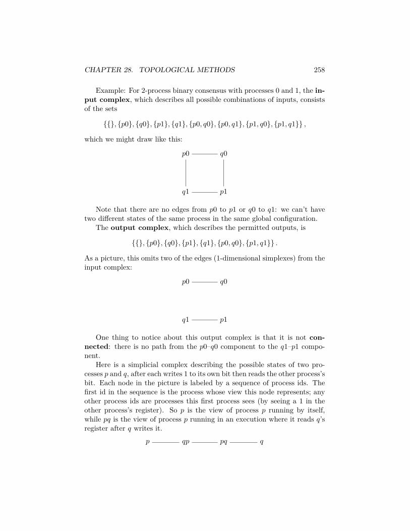
CHAPTER 28. TOPOLOGICAL METHODS 258
Example: For 2-process binary consensus with processes 0 and 1, the in-put complex, which describes all possible combinations of inputs, consistsof the sets
, p0, q0, p1, q1, p0, q0, p0, q1, p1, q0, p1, q1 ,
which we might draw like this:
p0 q0
q1 p1
Note that there are no edges from p0 to p1 or q0 to q1: we can’t havetwo different states of the same process in the same global configuration.
The output complex, which describes the permitted outputs, is
, p0, q0, p1, q1, p0, q0, p1, q1 .
As a picture, this omits two of the edges (1-dimensional simplexes) from theinput complex:
p0 q0
q1 p1
One thing to notice about this output complex is that it is not con-nected: there is no path from the p0–q0 component to the q1–p1 compo-nent.
Here is a simplicial complex describing the possible states of two pro-cesses p and q, after each writes 1 to its own bit then reads the other process’sbit. Each node in the picture is labeled by a sequence of process ids. Thefirst id in the sequence is the process whose view this node represents; anyother process ids are processes this first process sees (by seeing a 1 in theother process’s register). So p is the view of process p running by itself,while pq is the view of process p running in an execution where it reads q’sregister after q writes it.
p qp pq q

CHAPTER 28. TOPOLOGICAL METHODS 259
The edges express the constraint that if we both write before we read,then if I don’t see your value you must see mine (which is why there is nop–q edge), but all other combinations are possible. Note that this complexis connected: there is a path between any two points.
Here’s a fancier version in which each process writes its input (and re-members it), then reads the other process’s register (i.e., a one-round full-information protocol). We now have final states that include the process’sown id and input first, then the other process’s id and input if it is visible.For example, p1 means p starts with 1 but sees a null and q0p1 means qstarts with 0 but sees p’s 1. The general rule is that two states are compat-ible if p either sees nothing or q’s actual input and similarly for q, and thatat least one of p or q must see the other’s input. This gives the followingsimplicial complex:
p0 q0p0 p0q0 q0
q1p0
p0q1
q1
p1q0
q0p1
p1q1 q1p1 p1
Again, the complex is connected.The fact that this looks like four copies of the p–qp–pq–q complex pasted
into each edge of the input complex is not an accident: if we fix a pair ofinputs i and j, we get pi–qjpi–piqj–qj, and the corners are pasted togetherbecause if p sees only p0 (say), it can’t tell if it’s in the p0/q0 execution orthe p0/q1 execution.
The same process occurs if we run a two-round protocol of this form,where the input in the second round is the output from the first round.Each round subdivides one edge from the previous round into three edges:

CHAPTER 28. TOPOLOGICAL METHODS 260
p− q
p− qp− pq − q
p− (qp)p− p(qp)− qp− (pq)(qp)− (qp)(pq)− pq − q(pq)− (pq)q − q
Here (pq)(qp) is the view of p after seeing pq in the first round and seeingthat q saw qp in the first round.
28.3.2 Subdivisions
In the simple write-then-read protocol above, we saw a single input edge turninto 3 edges. Topologically, this is an example of a subdivision, where werepresent a simplex using several new simplexes pasted together that coverexactly the same points.
Certain classes of protocols naturally yield subdivisions of the inputcomplex. The iterated immediate snapshot (IIS) model, defined byBorowsky and Gafni [BG97], considers executions made up of a sequenceof rounds (the iterated part) where each round is made up of one or moremini-rounds in which some subset of the processes all write out their cur-rent views to their own registers and then take snapshots of all the registers(the immediate snapshot part). The two-process protocols of the previoussection are special cases of this model.
Within each round, each process p obtains a view vp that contains theprevious-round views of some subset of the processes. We can represent theviews as a subset of the processes, which we will abbreviate in pictures byputting the view owner first: pqr will be the view p, q, r as seen by p, whileqpr will be the same view as seen by q. The requirements on these viewsare that (a) every process sees its own previous view: p ∈ vp for all p; (b)all views are comparable: vp ⊆ vq or vq ⊆ vp; and (c) if I see you, then I seeeverything you see: q ∈ vp implies vq ⊆ vp. This last requirement is calledimmediacy and follows from the assumption that writes and snapshots aredone in the same mini-round: if I see your write, then your snapshot takesplace no later than mine does.
The IIS model does not correspond exactly to a standard shared-memorymodel (or even a standard shared-memory model augmented with cheapsnapshots). There are two reasons for this: standard snapshots don’t provide

CHAPTER 28. TOPOLOGICAL METHODS 261
immediacy, and standard snapshots allow processes to go back an performmore than one snapshot on the same object. The first issue goes away if weare looking at impossibility proofs, because the adversary can restrict itselfonly to those executions that satisfy immediacy. The second issue is moredelicate, but Borowsky and Gafni demonstrate that any decision protocolthat runs in the standard model can be simulated in the IIS model, using avariant of BG simulation.
For three processes, one round of immediate snapshots gives rise to thesimplicial complex depicted in Figure 28.1. The corners of the big triangleare the solo views of processes that do their snapshots before anybody elseshows up. Along the edges of the big triangle are views corresponding to 2-process executions, while in the middle are complete views of processes thatrun late enough to see everything. Each little triangle corresponds to someexecution. For example, the triangle with corners p, qp, rpq corresponds toa sequential execution where p sees nobody, q sees p, and r sees both p andq. The triangle with corners pqr, qpr, and rpq is the maximally-concurrentexecution where all three processes write before all doing their snapshots:here everybody sees everybody. It is not terribly hard to enumerate allpossible executions and verify that the picture includes all of them. In higherdimension, the picture is more complicated, but we still get a subdivisionthat preserves the original topological structure [BG97].
Figure 28.2 shows (part of) the next step of this process: here we havedone two iterations of immediate snapshot, and filled in the second-roundsubdivisions for the p–qpr–rpq and pqr–qpr–rpq triangles. (Please imaginesimilar subdivisions of all the other triangles that I was too lazy to fill inby hand.) The structure is recursive, with each first-level triangle mappingto an image of the entire first-level complex. As in the two-process case,adjacent triangles overlap because the relevant processes don’t have enoughinformation; for example, the points on the qpr–rpq edge correspond toviews of q or r that don’t include p in round 2 and so can’t tell whether psaw p or pqr in round 1.
The important feature of the round-2 complex (and the round-k complexin general) is that it’s a triangulation of the original outer triangle: apartition into little triangles where each corner aligns with corners of otherlittle triangles.
(Better pictures of this process in action can be found in Figures 25 and26 of [HS99].)

CHAPTER 28. TOPOLOGICAL METHODS 262
p
qr
rpq
qp
pq
rqqr
qpr
pqr
pr
rp
Figure 28.1: Subdivision corresponding to one round of immediate snapshot

CHAPTER 28. TOPOLOGICAL METHODS 263
p
qr
rpq
qp
pq
rqqr
qpr
pqr
pr
rp
Figure 28.2: Subdivision corresponding to two rounds of immediate snapshot

CHAPTER 28. TOPOLOGICAL METHODS 264
1
2 3
1
1
1 1
3
3
2
3
2
Figure 28.3: An attempt at 2-set agreement
28.4 Impossibility of k-set agreementNow let’s show that there is no way to do k-set agreement with n = k + 1processes in the IIS model.
Suppose that after some fixed number of rounds, each process choosesan output value. This output can only depend on the view of the process,so is fixed for each vertex in the subdivision. Also, the validity conditionmeans that a process can only choose an output that it can see among theinputs in its view. This means that at the corners of the outer triangle(corresponding to views where the process thinks it’s alone), a process mustreturn its input, while along the outer edges (corresponding to views wheretwo processes may see each other but not the third), a process must returnone of the two inputs that appear in the corners incident to the edge. Internalcorners correspond to views that include—directly or indirectly—the inputsof all processes, so these can be labeled arbitrarily. An example is given inFigure 28.3, for a one-round protocol with three processes.

CHAPTER 28. TOPOLOGICAL METHODS 265
We now run into Sperner’s Lemma [Spe28], which says that, for anysubdivision of a simplex into smaller simplexes, if each corner of the originalsimplex has a different color, and each corner that appears on some face ofthe original simplex has a color equal to the color of one of the corners ofthat face, then within the subdivision there are an odd number of simplexeswhose corners are all colored differently.3
How this applies to k-set agreement: Suppose we have n = k+1 processesin a wait-free system (corresponding to allowing up to k failures). Withthe cooperation of the adversary, we can restrict ourselves to executionsconsisting of ` rounds of iterated immediate snapshot for some ` (terminationcomes in here to show that ` is finite). This gives a subdivision of a simplex,where each little simplex corresponds to some particular execution and eachcorner some process’s view. Color all the corners of the little simplexes inthis subdivision with the output of the process holding the correspondingview. Validity means that these colors satisfy the requirements of Sperner’sLemma. Sperner’s Lemma then says that some little simplex has all k + 1colors, giving us a bad execution with more than k distinct output values.
The general result says that we can’t do k-set agreement with k failuresfor any n > k. We haven’t proved this result, but it can be obtained fromthe n = k + 1 version using a simulation of k + 1 processes with k failuresby n processes with k failures due to Borowsky and Gafni [BG93].
28.5 Simplicial maps and specificationsLet’s step back and look at consensus again.
3The proof of Sperner’s Lemma is not hard, and is done by induction on the dimensionk. For k = 0, any subdivision consists of exactly one zero-dimensional simplex whose singlecorner covers all k + 1 = 1 colors. For k + 1, suppose that the colors are 1, . . . , k + 1,and construct a graph with a vertex for each little simplex in the subdivision and anextra vertex for the region outside the big simplex. Put an edge in this graph betweeneach pair of regions that share a k-dimensional face with colors 1, . . . , k. The inductionhypothesis tells us that there are an odd number of edges between the outer-region vertexand simplexes on the 1, . . . , k-colored face of the big simplex. The Handshaking Lemmafrom graph theory says that the sum of the degrees of all the nodes in the graph is even.But this can only happen if there are an even number of nodes with odd degree, implyingthat the are are an odd number of simplexes in the subdivision with an odd number offaces colored 1, . . . , k.
Now suppose we have a simplex with at least one face f colored 1, . . . , k. If theopposite corner is colored c 6= k + 1, then it has exactly two faces colored 1, . . . , k: f ,and the face that replaces f ’s c-colored corner with the opposite corner. So the only wayto get an odd number of 1, . . . , k-colored faces is to have all k+ 1 colors. It follows thatthere are an odd number of (k + 1)-colored simplexes.

CHAPTER 28. TOPOLOGICAL METHODS 266
One thing we could conclude from the fact that the output complex forconsensus was not connected but the ones describing our simple protocolswere was that we can’t solve consensus (non-trivially) using these protocols.The reason is that to solve consensus using such a protocol, we would needto have a mapping from states to outputs (this is just whatever rule tellseach process what to decide in each state) with the property that if somecollection of states are consistent, then the outputs they are mapped to areconsistent.
In simplical complex terms, this means that the mapping from statesto outputs is a simplicial map, a function f from points in one simplicialcomplex C to points in another simplicial complex D such that for anysimplex A ∈ C, f(A) = f(x)|x ∈ A gives a simplex in D. (Recall thatconsistency is represented by including a simplex, in both the state complexand the output complex.) A mapping from states to outputs that satisfiesthe consistency requirements encoded in the output complex s always asimplicial map, with the additional requirement that it preserves process ids(we don’t want process p to decide the output for process q). Conversely,any id-preserving simplicial map gives an output function that satisfies theconsistency requirements.
Simplicial maps are examples of continuous functions, which have allsorts of nice topological properties. One nice property is that a continuousfunction can’t separate a connected space into disconnected components. Wecan prove this directly for simplical maps: if there is a path of 1-simplexesx1, x2, x2, x3, . . . xk−1, xk from x1 to xk in C, and f : C → D is asimplicial map, then there is a path of 1-simplexes f(x1), f(x2), . . . fromf(x1) to f(xk). Since being connected just means that there is a pathbetween any two points,4 if C is connected we’ve just shown that f(C) is aswell.
Getting back to our consensus example, it doesn’t matter what simplicialmap f you pick to map process states to outputs; since the state complex Cis connected, so is f(C), so it lies entirely within one of the two connectedcomponents of the output complex. This means in particular that everybodyalways outputs 0 or 1: the protocol is trivial.
28.5.1 Mapping inputs to outputs
For general decision tasks, it’s not enough for the outputs to be consistentwith each other. They also have to be consistent with the inputs. This can
4Technically, this is the definition of path-connected, which is the same as connectedfor well-behaved topological spaces.

CHAPTER 28. TOPOLOGICAL METHODS 267
be expressed by a relation ∆ between input simplexes and output simplexes.Formally, a decision task is modeled by a triple (I,O,∆), where I is the
input complex, O is the output complex, and (A,B) ∈ ∆ if and only if B isa permissible output given input I. Here there are no particular restrictionson ∆ (for example, it doesn’t have to be a simplicial map or even a function),but it probably doesn’t make sense to look at decision tasks unless there isat least one permitted output simplex for each input simplex.
28.6 The asynchronous computability theoremGiven a decision task specified in this way, there is a topological characteriza-tion of when it has a wait-free solution. This is given by the AsynchronousComputability Theorem (Theorem 3.1 in [HS99]), which says:
Theorem 28.6.1. A decision task (I,O,∆) has a wait-free protocol usingshared memory if and only if there exists a chromatic subdivision σ of I anda color-preserving simplicial map µ : σ(I)→ O such that for each simplex sin σ(I), µ(S) ∈ ∆(carrier(S, I)).
To unpack this slightly, a chromatic subdivision is a subdivision whereeach vertex is labeled by a process id (a color), and no simplex has twovertices with the same color. A color-preserving simplicial map is a simplicialmap that preserves ids. The carrier of a simplex in a subdivision is whateveroriginal simplex it is part of. So the theorem says that I can only solve atask if I can find a simplicial map from a subdivision of the input complexto the output complex that doesn’t do anything strange to process ids andthat is consistent with ∆.
Looking just at the theorem, one might imagine that the proof consistsof showing that the protocol complex defined by the state complex afterrunning the protocol to completion is a subdivision of the input complex,followed by the same argument we’ve seen already about mapping the statecomplex to the output complex. This is almost right, but it’s complicated bytwo inconvenient facts: (a) the state complex generally isn’t a subdivision ofthe input complex, and (b) if we have a map from an arbitrary subdivisionof the input complex, it is not clear that there is a corresponding protocolthat produces this particular subdivision.
So instead the proof works like this:
Protocol implies map Even though we don’t get a subdivision with thefull protocol, there is a restricted set of executions that does give a

CHAPTER 28. TOPOLOGICAL METHODS 268
subdivision. So if the protocol works on this restricted set of execu-tions, an appropriate map exists. There are two ways to prove this:Herlihy and Shavit do so directly, by showing that this restricted setof executions exists, and Borowksy and Gafni [BG97] do so indirectly,by showing that the IIS model (which produces exactly the standardchromatic subdivision used in the ACT proof) can simulate an ordi-nary snapshot model. Both methods are a bit involved, so we will skipover this part.
Map implies protocol This requires an algorithm. The idea here is thatthat participating set algorithm, originally developed to solve k-setagreement [BG93], produces precisely the standard chromatic subdivi-sion used in the ACT proof. In particular, it can be used to solve theproblem of simplex agreement, the problem of getting the processesto agree on a particular simplex contained within the subdivision oftheir original common input simplex. This is a little easier to explain,so we’ll do it.
28.6.1 The participating set protocol
Algorithm 28.1 depicts the participating set protocol; this first appearedin [BG93], although the presentation here is heavily influenced by the versionin Elizabeth Borowsky’s dissertation [Bor95]. The shared data consists ofa snapshot object level, and processes start at a high level and float downuntil they reach a level i such that there are already i processes at this levelor below. The set returned by a process consists of all processes it sees atits own level or below, and it can be shown that this in fact implements aone-shot immediate snapshot. Since immediate snapshots yield a standardsubdivision, this gives us what we want for converting a color-preservingsimplicial map to an actual protocol.
1 Initially, level[i] = n+ 2 for all i.2 repeat3 level[i]← level[i]− 14 v ← snapshot(level)5 S ← j | v[j] ≤ level[i]6 until |S| ≥ level[i]7 |S| ≥ level[i] return S
Algorithm 28.1: Participating set

CHAPTER 28. TOPOLOGICAL METHODS 269
The following theorem shows that the return values from participatingset have all the properties we want for iterated immediate snapshot:
Theorem 28.6.2. Let Si be the output of the participating set algorithm forprocess i. Then all of the following conditions hold:
1. For all i, i ∈ Si. (Self-containment.)
2. For all i, j, Si ⊆ Sj or Sj ⊆ Si. (Atomic snapshot.)
3. For all i, j, if i ∈ Sj, then Si ⊆ Sj. (Immediacy.)
Proof. Self-inclusion is trivial, but we will have to do some work for theother two properties.
The first step is to show that Algorithm 28.1 neatly sorts the processesout into levels, where each process that returns at level k returns preciselythe set of processes at level k and below.
For each process i, let Si be defined as above, let `i be the final value oflevel[i] when i returns, and let S′i = j | `j ≤ Si. Our goal is to show thatS′i = Si, justifying the above claim.
Because no process ever increases its level, if process i observes level[j] ≤`i in its last snapshot, then `j ≤ level[j] ≤ `i. So S′i is a superset of Si. Wethus need to show only that no extra processes sneak in; in particular, wewill to show that Si = S′i, by showing that both equal `i.
The first step is to show that |S′i| ≥ |Si| ≥ `i. The first inequality followsfrom the fact that S′i ⊇ Si; the second follows from the code (if not, i wouldhave stayed in the loop).
The second step is to show that |S′i| ≤ `i. Suppose not; that is, supposethat |S′i| > `i. Then there are at least `i+1 processes with level `i or less, allof which take a snapshot on level `i + 1. Let i′ be the last of these processesto take a snapshot while on level `i+ 1. Then i′ sees at least `i+ 1 processesat level `i + 1 or less and exits, contradicting the assumption that it reacheslevel `i. So |S′i| ≤ `i.
The atomic snapshot property follows immediately from the fact that if`i ≤ `j , then `k ≤ `i implies `k ≤ `j , giving Si = S′i ⊆ S′j = Sj . Similarly,for immediacy we have that if i ∈ Sj , then `i ≤ `j , giving Si ≤ Sj by thesame argument.
The missing piece for turning this into IIS is that in Algorithm 28.1, Ionly learn the identities of the processes I am supposed to include but nottheir input values. This is easily dealt with by adding an extra register foreach process, to which it writes its input before executing participating set.

CHAPTER 28. TOPOLOGICAL METHODS 270
28.7 Proving impossibility resultsTo show something is impossible using the ACT, we need to show that thereis no color-preserving simplicial map from a subdivision of I to O satisfyingthe conditions in ∆. This turns out to be equivalent to showing that thereis no continuous function from I to O with the same properties, becauseany such simplicial map can be turned into a continuous function (on thegeometric version of I, which includes the intermediate points in additionto the corners). Fortunately, topologists have many tools for proving non-existence of continuous functions.
28.7.1 k-connectivity
Define them-dimensional disk to be the set of all points at most 1 unit awayfrom the origin in Rm, and the m-dimensional sphere to be the surface ofthe (m + 1)-dimensional disk (i.e., all points exactly 1 unit away from theorigin in Rm+1). Note that what we usually think of as a sphere (a solidbody), topologists call a disk, leaving the term sphere for just the outsidepart.
An object is k-connected if any continuous image of an m-dimensionalsphere can be extended to a continuous image of an (m + 1)-dimensionaldisk, for all m ≤ k.5 This is a roundabout way of saying that if we candraw something that looks like a deformed sphere inside our object, we canalways include the inside as well: there are no holes that get in the way.The punch line is that continuous functions preserve k-connectivity: if wemap an object with no holes into some other object, the image had betternot have any holes either.
Ordinary path-connectivity is the special case when k = 0; here, the0-sphere consists of two points and the 1-disk is the path between them. So0-connectivity says that for any two points, there is a path between them.
For 1-connectivity, if we draw a loop (a path that returns to its origin), wecan include the interior of the loop somewhere. One way to thinking aboutthis is to say that we can shrink the loop to a point without leaving the object(the technical term for this is that the path is null-homotopic, where ahomotopy is a way to transform one thing continuously into another thingover time and the null path sits on a single point). An object that is1-connected is also called simply connected.
5This definition is for the topological version of k-connectivity. It is not related in anyway to the definition of k-connectivity in graph theory, where a graph is k-connected ifthere are k disjoint paths between any two points.
CHAPTER 28. TOPOLOGICAL METHODS 271
For 2-connectivity, we can’t contract a sphere (or box, or the surface ofa 2-simplex, or anything else that looks like a sphere) to a point.
The important thing about k-connectivity is that it is possible to provethat any subdivision of a k-connected simplicial complex is also k-connected(sort of obvious if you think about the pictures, but it can also be provedformally), and that k-connectivity is preserved by simplicial maps (if not,somewhere in the middle of all the k-simplexes representing our surface is a(k+1)-simplex in the domain that maps to a hole in the range, violating therule that simplicial maps map simplexes to simplexes). So a quick way toshow that the Asynchronous Computability Theorem implies that somethingis not asynchronously computable is to show that the input complex is k-connected and the output complex isn’t.
28.7.2 Impossibility proofs for specific problems
Here are some applications of the Asynchronous Computability Theoremand k-connectivity:
Consensus There is no nontrivial wait-free consensus protocol for n ≥ 2processes. Proof: The input complex is 1-connected, but the outputcomplex is not, and we need a map that covers the entire outputcomplex (by nontriviality).
k-set agreement There is no wait-free k-set agreement for n ≥ k + 1processes. Proof: The output complex for k-set agreement is not k-connected, because buried inside it are lots of (k+1)-dimensional holescorresponding to missing simplexes where all k + 1 processes choosedifferent values. But these holes aren’t present in the input complex—it’s OK if everybody starts with different inputs—and the validityrequirements for k-set agreement force us to map the surfaces of thesenon-holes around holes in the output complex. (This proof actuallyturns into the Sperner’s Lemma proof if we fully expand the claimabout having to map the input complex around the hole.)
Renaming There is no wait-free renaming protocol with less than 2n − 1output names for all n. The general proof of this requires showing thatwith fewer names we get holes that are too big (and ultimately reducesto Sperner’s Lemma); for the special case of n = 3 and m = 4, seeFigure 28.4, which shows how the output complex of renaming foldsup into the surface of a torus. This means that renaming for n = 3

CHAPTER 28. TOPOLOGICAL METHODS 272
a1 b2
c3 a4
c1
b1 c2
b3
a2
c4
b1
a1
a3
b2
c2
c1
b4
a1
a2
c3
b1
Figure 28.4: Output complex for renaming with n = 3, m = 4. Each vertexis labeled by a process id (a, b, c) and a name (1, 2, 3, 4). Observe that theleft and right edges of the complex have the same sequence of labels, as dothe top and bottom edges; the complex thus folds up into a (twisted) torus.(This is a poor imitation of part of [HS99, Figure 9].)
and m = 4 is exactly the same as trying to stretch a basketball intoan inner tube.

Chapter 29
Approximate agreement
1The approximate agreement [DLP+86] or ε-agreement problem is
another relaxation of consensus where input and output values are real num-bers, and a protocol is required to satisfy modified validity and agreementconditions.
Let xi be the input of process i and yi its output. Then a protocolsatisfies approximate agreement if it satisfies:
Termination Every nonfaulty process eventually decides.
Validity Every process returns an output within the range of inputs. For-mally, for all i, it holds that (minj xj) ≤ yi ≤ (maxj xj).
ε-agreement For all i and j, |i− j| ≤ ε.
Unlike consensus, approximate agreement has wait-free algorithms forasynchronous shared memory, which we’ll see in §29.1). But a curious prop-erty of approximate agreement is that it has no bounded wait-free algo-rithms, even for two processes (see §29.2)
29.1 Algorithms for approximate agreementNot only is approximate agreement solvable, it’s actually easily solvable, tothe point that there are many known algorithms for solving it.
We’ll use the algorithm of Moran [Mor95], mostly as presented in [AW04,
273

CHAPTER 29. APPROXIMATE AGREEMENT 274
Algorithm 54] but with a slight bug fix;1 pseudocode appears in Algo-rithm 29.1.2
The algorithm carries out a sequence of asynchronous rounds in whichprocesses adopt new values, such that the spread of the vector of all valuesVr in round r, defined as spreadVr = max Vr−minVr, drops by a factor of 2per round. This is done by having each process choose a new value in eachround by taking the midpoint (average of min and max) of all the values itsees in the previous round. Slow processes will jump to the maximum roundthey see rather than propagating old values up from ancient rounds; thisis enough to guarantee that latecomer values that arrive after some processwrites in round 2 are ignored.
The algorithm uses a single snapshot object A to communicate, and eachprocess stores its initial input and a round number along with its currentpreference. We assume that the initial values in this object all have roundnumber 0, and that log2 0 = −∞ (which avoids a special case in the termi-nation test).
1 A[i]← 〈xi, 1, xi〉2 repeat3 〈x′1, r1, v1〉 . . . 〈x′n, rn, vn〉 ← snapshot(A)4 rmax ← maxj rj5 v ← midpointvj | rj = rmax6 A[i]← 〈xi, rmax + 1, v〉7 until rmax ≥ 2 and rmax ≥ log2(spread(x′j)/ε)8 return v
Algorithm 29.1: Approximate agreement
To show this works, we want to show that the midpoint operation guar-antees that the spread shrinks by a factor of 2 in each round. Let Vr be theset of all values v that are ever written to the snapshot object with round
1The original algorithm from [AW04] does not include the test rmax ≥ 2. This allowsfor bad executions in which process 1 writes its input of 0 in round 1 and takes a snapshotthat includes only its own input, after which process 2 runs the algorithm to completionwith input 1. Here process 2 will see 0 and 1 in round 1, and will write (1/2, 2, 1) toA[2]; on subsequent iterations, it will see only the value 1/2 in the maximum round, andafter dlog2(1/ε)e rounds it will decide on 1/2. But if we now wake process 1 up, it willdecided 0 immediately based on its snapshot, which includes only its own input and givesspread(x) = 0. Adding the extra test prevents this from happening, as new values thatarrive after somebody writes round 2 will be ignored.
2Showing that this particular algorithm works takes a lot of effort. If I were to do thisover, I’d probably go with a different algorithm due to Schenk [Sch95].

CHAPTER 29. APPROXIMATE AGREEMENT 275
number r. Let Ur ⊆ Vr be the set of values that are ever written to the snap-shot object with round number r before some process writes a value withround number r + 1 or greater; the intuition here is that Ur includes onlythose values that might contribute to the computation of some round-(r+1)value.Lemma 29.1.1. For all r for which Vr+1 is nonempty,
spread(Vr+1) ≤ spread(Ur)/2.Proof. Let U ir be the set of round-r values observed by a process i in theiteration in which it sees rmax = r in some iteration, if such an iterationexists. Note that U ir ⊆ Ur, because if some value with round r+1 or greateris written before i’s snapshot, then i will compute a larger value for rmax.
Given two processes i and j, we can argue from the properties of snapshotthat either U ir ⊆ U jr or U jr ⊆ U ir. The reason is that if i’s snapshot comesfirst, then j sees at least as many round-r values as i does, because the onlyway for a round-r value to disappear is if it is replaced by a value in a laterround. But in this case, process j will compute a larger value for rmax andwill not get a view for round r. The same holds in reverse if j’s snapshotcomes first.
Observe that if U ir ⊆ U jr , then∣∣∣midpoint(U ir)−midpoint(U jr )∣∣∣ ≤ spread(U jr )/2.
This holds because midpoint(U ir) lies within the interval[minU jr ,maxU jr
],
and every point in this interval is within spread(U jr )/2 of midpoint(U jr ). Thesame holds if U jr ⊆ U ir. So any two values written in round r+ 1 are withinspread(Ur)/2 of each other.
In particular, the minimum and maximum values in Vr+1 are withinspread(Ur)/2 of each other, so spread(Vr+1) ≤ spread(Ur)/2.
Corollary 29.1.2. For all r ≥ 2 for which Vr is nonempty,spread(Vr) ≤ spread(U1)/2r−1.
Proof. By induction on r. For r = 2, this is just Lemma 29.1.1. For largerr, use the fact that Ur−1 ⊆ Vr−1 and thus spread(Ur−1) ≤ spread(Vr−1) tocompute
spread(Vr) ≤ spread(Ur−1)/2≤ spread(Vr−1)/2≤ (spread(U1)/2r−2)/2= spread(U1)/2r−1.

CHAPTER 29. APPROXIMATE AGREEMENT 276
Let i be some process that finishes in the fewest number of rounds. Pro-cess i can’t finish until it reaches round rmax+1, where rmax ≥ log2(spread(x′j)/ε)for a vector of input values x′ that it reads after some process writes round2 or greater. We have spread(x′j) ≥ spread(U1), because every value inU1 is included in x′. So rmax ≥ log2 (spread(U1)/ε) and spread(Vrmax+1) ≤spread(U1)/2rmax ≤ spread(U1)/(spread(U1)/ε) = ε. Since any value re-turned is either included in Vrmax+1 or some later Vr′ ⊆ Vrmax+1, this givesus that the spread of all the outputs is less than ε: Algorithm 29.1 solvesapproximate agreement.
The cost of Algorithm 29.1 depends on the cost of the snapshot oper-ations, on ε, and on the initial input spread D. For linear-cost snapshots,this works out to O(n log(D/ε)).
29.2 Lower bound on step complexityThe dependence on D/ε is necessary, at least for deterministic algorithms.Here we give a lower bound due to Herlihy [Her91a], which shows thatany deterministic approximate agreement algorithm takes at least log3(D/ε)total steps even with just two processes.
Define the preference of a process in some configuration as the value itwill choose if it runs alone starting from this configuration. The preferenceof a process p is well-defined because the process is deterministic; it also canonly change as a result of a write operation by another process q (becauseno other operations are visible to p, and p’s own operations can’t changeits preference). The validity condition means that in an initial state, eachprocess’s preference is equal to its input.
Consider an execution with two processes p and q, where p starts withpreference p0 and q starts with preference q0. Run p until it is about toperform a write that would change q’s preference. Now run q until it isabout to change p’s preference. If p’s write no longer changes q’s preference,start p again and repeat until both p and q have pending writes that willchange the other process’s preference. Let p1 and q1 be the new preferencesthat result from these operations. The adversary can now choose betweenrunning P only and getting to a configuration with preferences p0 and q1,Q only and getting p1 and q0, or both and getting p1 and q1; each of thesechoices incurs at least one step. By the triangle inequality, |p0 − q0| ≤|p0 − q1| + |q1 − p1| + |p1 − q0|, so at least on of these configurations hasa spread between preferences that is at least 1/3 of the initial spread. It
CHAPTER 29. APPROXIMATE AGREEMENT 277
follows that after k steps the best spread we can get is D/3k, requiringk ≥ log3(D/ε) steps to get ε-agreement.
Herlihy uses this result to show that there are decisions problems thathave wait-free but not bounded wait-free deterministic solutions using regis-ters. Curiously, the lower bound says nothing about the dependence on thenumber of processes; it is conceivable that there is an approximate agree-ment protocol with running time that depends only on D/ε and not n.

Appendix
278

Appendix A
Assignments
Assignments are typically due Wednesdays at 5:00pm. Assignments can beturned in to Ennan Zhai’s mailbox on the first floor of AKW.
A.1 Assignment 1: due Wednesday, 2014-01-29,at 5:00pm
Bureaucratic part
Send me email! My address is [email protected] your message, include:
1. Your name.
2. Your status: whether you are an undergraduate, grad student, auditor,etc.
3. Anything else you’d like to say.
(You will not be graded on the bureaucratic part, but you should do itanyway.)
A.1.1 Counting evil processes
A connected bidirectional asynchronous network of n processes with iden-tities has diameter D and may contain zero or more evil processes. Fortu-nately, the evil processes, if they exist, are not Byzantine, fully conform toRFC 3514 [Bel03], and will correctly execute any code we provide for them.
279

APPENDIX A. ASSIGNMENTS 280
Suppose that all processes wake up at time 0 and start whatever protocolwe have given them. Suppose that each process initially knows whether it isevil, and knows the identities of all of its neighbors. However, the processesdo not know the number of processes n or the diameter of the network D.
Give a protocol that allows every process to correctly return the numberof evil processes no later than time D. Your protocol should only return avalue once for each process (no converging to the correct answer after aninitial wrong guess).
Solution
There are a lot of ways to do this. Since the problem doesn’t ask aboutmessage complexity, we’ll do it in a way that optimizes for algorithmic sim-plicity.
At time 0, each process initiates a separate copy of the flooding algorithm(Algorithm 4.1). The message 〈p,N(p), e〉 it distributes consists of its ownidentity, the identities of all of its neighbors, and whether or not it is evil.
In addition to the data for the flooding protocol, each process tracks aset I of all processes it has seen that initiated a protocol and a set N of allprocesses that have been mentioned as neighbors. The initial values of thesesets for process p are p and N(p), the neighbors of p.
Upon receiving a message 〈q,N(q), e〉, a process adds q to I and N(q) toN . As soon as I = N , the process returns a count of all processes for whiche = true.
Termination by D: Follows from the same analysis as flooding. Anyprocess at distance d from p has p ∈ I by time d, so I is complete by timeD.
Correct answer: Observe that N =⋃i∈I N(i) always. Suppose that
there is some process q that is not in I. Since the graph is connected, thereis a path from p to q. Let r be the last node in this path in I, and let s bethe following node. Then s ∈ N \ I and N 6= I. By contraposition, if I = Nthen I contains all nodes in the network, and so the count returned at thistime is correct.
A.1.2 Avoiding expensive processes
Suppose that you have a bidirectional but not necessarily complete asyn-chronous message-passing network represented by a graph G = (V,E) whereeach node in V represents a process and each edge in E connects two pro-cesses that can send messages to each other. Suppose further that each

APPENDIX A. ASSIGNMENTS 281
process is assigned a weight 1 or 2. Starting at some initiator process, we’dlike to construct a shortest-path tree, where each process points to one ofits neighbors as its parent, and following the parent pointers always gives apath of minimum total weight to the initiator.1
Give a protocol that solves this problem with reasonable time, message,and bit complexity, and show that it works.
Solution
There’s an ambiguity in the definition of total weight: does it include theweight of the initiator and/or the initial node in the path? But since thesevalues are the same for all paths to the initiator from a given process, theydon’t affect which is lightest.
If we don’t care about bit complexity, there is a trivial solution: Use anexisting BFS algorithm followed by convergecast to gather the entire struc-ture of the network at the initiator, run your favorite single-source shortest-path algorithm there, then broadcast the results. This has time complexityO(D) and message complexity O(DE) if we use the BFS algorithm from§5.3. But the last couple of messages in the convergecast are going to bepretty big.
A solution by reduction: Suppose that we construct a new graph G′
where each weight-2 node u inG is replaced by a clique of nodes u1, u2, . . . uk,with each node in the clique attached to a different neighbor of u. We thenrun any breadth-first search protocol of our choosing on G′, where eachweight-2 node simulates all members of the corresponding clique. Becauseany path that passes through a clique picks up an extra edge, each path inthe breadth-first search tree has a length exactly equal to the sum of theweights of the nodes other than its endpoints.
A complication is that if I am simulating k nodes, between them theymay have more than one parent pointer. So we define u.parent to be ui.parentwhere ui is a node at minimum distance from the initiator in G′. We alsore-route any incoming pointers to uj 6= ui to point to ui instead. Becauseui was chosen to have minimum distance, this never increases the length ofany path, and the resulting modified tree is a still a shortest-path tree.
Adding nodes blows up |E′|, but we don’t need to actually send messagesbetween different nodes ui represented by the same process. So if we use the
1Clarification added 2014-01-26: The actual number of hops is not relevant for theconstruction of the shortest-path tree. By shortest path, we mean path of minimum totalweight.

APPENDIX A. ASSIGNMENTS 282
§5.3 algorithm again, we only send up to D messages per real edge, givingO(D) time and O(DE) messages.
If we don’t like reductions, we could also tweak one of our existing al-gorithms. Gallager’s layered BFS (§5.2) is easily modified by changing thedepth bound for each round to a total-weight bound. The synchronizer-based BFS can also be modified to work, but the details are messy.
A.2 Assignment 2: due Wednesday, 2014-02-12,at 5:00pm
A.2.1 Synchronous agreement with weak failures
Suppose that we modify the problem of synchronous agreement with crashfailures from Chapter 7 so that instead of crashing a process forever, theadversary may jam some or all of its outgoing messages for a single round.The adversary has limited batteries on its jamming equipment, and canonly cause f such one-round faults. There is no restriction on when theseone-round jamming faults occur: the adversary might jam f processes forone round, one process for f rounds, or anything in between, so long as thesum over all rounds of the number of processes jammed in each round is atmost f . For the purposes of agreement and validity, assume that a processis non-faulty if it is never jammed.2
As a function of f and n, how many rounds does it take to reach agree-ment in the worst case in this model, under the usual assumptions thatprocesses are deterministic and the algorithm must satisfy agreement, ter-mination, and validity? Give the best upper and lower bounds that youcan.
Solution
The par solution for this is an Ω(√f) lower bound and O(f) upper bound.
I don’t know if it is easy to do better than this.For the lower bound, observe that the adversary can simulate an ordinary
crash failure by jamming a process in every round starting in the round itcrashes in. This means that in an r-round protocol, we can simulate k crashfailures with kr jamming faults. From the Dolev-Strong lower bound [DS83]
2 Clarifications added 2014-02-10: We assume that processes don’t know that they arebeing jammed or which messages are lost (unless the recipient manages to tell them thata message was not delivered). As in the original model, we assume a complete networkand that all processes have known identities.

APPENDIX A. ASSIGNMENTS 283
(see also Chapter 7), we know that there is no r-round protocol with k = rcrash failures faults, so there is no r-round protocol with r2 jamming faults.This gives a lower bound of
⌊√f⌋
+ 1 on the number of rounds needed tosolve synchronous agreement with f jamming faults.3
For the upper bound, have every process broadcast its input every round.After f+1 rounds, there is at least one round in which no process is jammed,so every process learns all the inputs and can take, say, the majority value.
A.2.2 Byzantine agreement with contiguous faults
Suppose that we restrict the adversary in Byzantine agreement to corruptinga connected subgraph of the network; the idea is that the faulty nodes needto coordinate, but can’t relay messages through the non-faulty nodes to doso.
Assume the usual model for Byzantine agreement with a network in theform of an m ×m torus. This means that each node has a position (x, y)in 0, . . . ,m− 1 × 0, . . . ,m− 1, and its neighbors are the four nodes(x+ 1 mod m, y), (x−1 mod m, y), (x, y+ 1 mod m), and (x, y−1 mod m).
For sufficiently large m,4 what is the largest number of faults f ; thatthis system can tolerate and still solve Byzantine agreement?
Solution
The relevant bound here is the requirement that the network have enoughconnectivity that the adversary can’t take over half of a vertex cut (see§8.1.3). This is complicated slightly by the requirement that the faultynodes be contiguous.
The smallest vertex cut in a sufficiently large torus consists of the fourneighbors of a single node; however, these nodes are not connected. But wecan add a third node to connect two of them (see Figure A.1).
By adapting the usual lower bound we can use this construction to showthat f = 3 faults are enough to prevent agreement when m ≥ 3. Thequestion then is whether f = 2 faults is enough.
By a case analysis, we can show that any two nodes in a sufficientlylarge torus are either adjacent themselves or can be connected by threepaths, where no two paths have adjacent vertices. Assume without loss of
3Since Dolev-Strong only needs to crash one process per round, we don’t really needthe full r jamming faults for processes that crash late. This could be used to improve theconstant for this argument.
4Problem modified 2014-02-03. In the original version, it asked to compute f for allm, but there are some nasty special cases when m is small.

APPENDIX A. ASSIGNMENTS 284
Figure A.1: Connected Byzantine nodes take over half a cut
generality that one of the nodes is at position (0, 0). Then any other nodeis covered by one of the following cases:
1. Nodes adjacent to (0, 0). These can communicate directly.
2. Nodes at (0, i) or (i, 0). These cases are symmetric, so we’ll describethe solution for (0, i). Run one path directly north: (0, 1), (0, 2), . . . , (0, i−1). Similarly, run a second path south: (0,−1), (0,−2), . . . (0, i + 1).For the third path, take two steps east and then run north and backwest: (1, 0), (2, 0), (2, 1), (2, 2), . . . , (2, i), (1, i). These paths are allnon-adjacent as long as m ≥ 4.
3. Nodes at (±1, i) or (i,±1), where i is not −1, 0, or 1. Suppose the nodeis at (1, i). Run one path east then north through (1, 0), (1, 1), . . . , (1, i−1). The other two paths run south and west, with a sideways jog in themiddle as needed. This works for m sufficiently large to make roomfor the sideways jogs.
4. Nodes at (±1,±1) or (i, j) where neither of i or j is −1, 0, or 1. Now wecan run one path north then east, one east then north, one south thenwest, and one west then south, creating four paths in a figure-eightpattern centered on (0, 0).
A.3 Assignment 3: due Wednesday, 2014-02-26,at 5:00pm
A.3.1 Among the elect
The adversary has decided to be polite and notify each non-faulty processeswhen he gives up crashing it. Specifically, we have the usual asynchronousmessage-passing system with up to f faulty processes, but every non-faultyprocess is eventually told that it is non-faulty. (Faulty processes are toldnothing.)

APPENDIX A. ASSIGNMENTS 285
For what values of f can you solve consensus in this model?
Solution
We can tolerate f < n/2, but no more.If f < n/2, the following algorithm works: Run Paxos, where each
process i waits to learn that it is non-faulty, then acts as a proposer forproposal number i. The highest-numbered non-faulty process then carriesout a proposal round that succeeds because no higher proposal is ever issued,and both the proposer (which is non-faulty) and a majority of acceptersparticipate.
If f ≥ n/2, partition the processes into two groups of size bn/2c, withany leftover process crashing immediately. Make all of the processes in bothgroups non-faulty, and tell each of them this at the start of the protocol.Now do the usual partitioning argument: Run group 0 with inputs 0 with nomessages delivered from group 1 until all processes decide 0 (we can do thisbecause the processes can’t distinguish this execution from one in whichthe group 1 processes are in fact faulty). Run group 1 similarly until allprocesses decide 1. We have then violated agreement, assuming we didn’tpreviously violate termination of validity.
A.3.2 Failure detectors on the cheap
Suppose we do not have the budget to equip all of our machines with failuredetectors. Instead, we order an eventually strong failure detector for kmachines, and the remaining n− k machines get fake failure detectors thatnever suspect anybody. The choice of which machines get the real failuredetectors and which get the fake ones is under the control of the adversary.
This means that every faulty process is eventually permanently suspectedby every non-faulty process with a real failure detector, and there is atleast one non-faulty process that is eventually permanently not suspectedby anybody. Let’s call the resulting failure detector ♦Sk.
Let f be the number of actual failures. Under what conditions on f , k,and n can you still solve consensus in the usual deterministic asynchronousmessage-passing model using ♦Sk?
Solution
First observe that ♦S can simulate ♦Sk for any k by having n− k processesignore the output of their failure detectors. So we need f < n/2 by theusual lower bound on ♦S.

APPENDIX A. ASSIGNMENTS 286
If f ≥ k, we are also in trouble. The f > k case is easy: If there existsa consensus protocol for f > k, then we can transform it into a consensusprotocol for n − k processes and f − k failures, with no failure detectorsat all, by pretending that there are an extra k processes with real failuredetectors that crash immediately. The FLP impossibility result rules thisout.
If f = k, we have to be a little more careful. By immediately crashingf − 1 processes with real failure detectors, we can reduce to the f = k = 1case. Now the adversary runs the FLP strategy. If no processes crash, thenall n− k + 1 surviving process report no failures; if it becomes necessary tocrash a process, this becomes the one remaining process with the real failuredetector. In either case the adversary successfully prevents consensus.
So let f < k. Then we have weak completeness, because every faultyprocess is eventually permanently suspected by at least k−f > 0 processes.We also have weak accuracy, because it is still the case that some processis eventually permanently never suspected by anybody. By boosting weakcompleteness to strong completeness as described in §11.2.3, we can turnout failure detector into ♦S, meaning we can solve consensus precisely whenf < min(k, n/2).
A.4 Assignment 4: due Wednesday, 2014-03-26,at 5:00pm
A.4.1 A global synchronizer with a global clock
Consider an asynchronous message-passing system with n processes in abidirectional ring with no failures. Suppose that the processes are equippedwith a global clock, which causes a local event to occur simultaneously ateach process every c time units, where as usual 1 is the maximum messagedelay. We would like to use this global clock to build a global synchronizer.Provided c is at least 1, a trivial approach is to have every process advanceto the next round whenever the clock pulse hits. This gives one synchronousround every c time units.
Suppose that c is greater than 1 but still o(n). Is it possible to builda global synchronizer in this model that runs more than a constant ratiofaster than this trivial global synchronizer in the worst case?

APPENDIX A. ASSIGNMENTS 287
A.4.2 A message-passing counter
A counter is a shared object that support operations inc and read, whereread returns the number of previous inc operations.
Algorithm A.1 purports to implement a counter in an asynchronousmessage-passing system subject to f < n/2 crash failures. In the algo-rithm, each process i maintains a vector ci of contributions to the counterfrom all the processes, as well as a nonce ri used to distinguish responses todifferent read operations from each other. All of these values are initiallyzero.
Show that the implemented counter is linearizable, or give an exampleof an execution where it isn’t.
1 procedure inc2 ci[i]← ci[i] + 13 Send ci[i] to all processes.4 Wait to receive ack(ci[i]) from a majority of processes.5 upon receiving c from j do6 ci[j]← max(ci[j], c)7 Send ack(c) to j.8 procedure read9 ri ← ri + 1
10 Send read(ri) to all processes.11 Wait to receive respond(ri, cj) from a majority of processes j.12 return
∑k maxj cj [k]
13 upon receiving read(r) from j do14 Send respond(r, ci) to j
Algorithm A.1: Counter algorithm for Problem A.4.2.
A.5 Assignment 5: due Wednesday, 2014-04-09,at 5:00pm
A.5.1 A concurrency detector
Consider the following optimistic mutex-like object, which we will call aconcurrency detector. A concurrency detector supports two operationsfor each process i, enteri and exiti. These operations come in pairs: a

APPENDIX A. ASSIGNMENTS 288
process enters a critical section by executing enteri, and leaves by executingexiti. The behavior of the object is undefined if a process calls enteri twicewithout an intervening exiti, or calls exiti without first calling enteri.
Unlike mutex, a concurrency detector does not enforce that only oneprocess is in the critical section at a time; instead, exiti returns 1 if theinterval between it and the previous enteri overlaps with some intervalbetween a enterj and corresponding exitj for some j 6= i, and returns 0 ifthere is no overlap.
Is there a deterministic linearizable wait-free implementation of a con-currency detector from atomic registers? If there is, give an implementation.If there is not, give an impossibility proof.
Solution
It is not possible to implement this object using atomic registers.Suppose that there were such an implementation. Algorithm A.2 im-
plements two-process consensus using a two atomic registers and a singleconcurrency detector, initialized to the state following enter1.
1 procedure consensus1(v)2 r1 ← v3 if exit1() = 1 then4 return r25 else6 return v
7 procedure consensus2(v)8 r2 ← v9 enter2()
10 if exit2() = 1 then11 return v12 else13 return r1
Algorithm A.2: Two-process consensus using the object from Prob-lem A.5.1
Termination is immediate from the absence of loops in the code.To show validity and termination, observe that one of two cases holds:
1. Process 1 executes exit1 before process 2 executes enter2. In this

APPENDIX A. ASSIGNMENTS 289
case there is no overlap between the interval formed by the implicitenter1 and exit1 and the interval formed by enter2 and exit2. Sothe exit1 and exit2 operations both return 0, causing process 1 toreturn its own value and process 2 to return the contents of r1. Thesewill equal process 1’s value, because process 2’s read follows its call toenter2, which follows exit1 and thus process 1’s write to r1.
2. Process 1 executes exit1 after process 2 executes enter2. Now bothexit operations return 1, and so process 2 returns its own value whileprocess 1 returns the contents of r2, which it reads after process 2writes its value there.
In either case, both processes return the value of the first process toaccess the concurrency detector, satisfying both agreement and validity.This would give a consensus protocol for two processes implemented fromatomic registers, contradicting the impossibility result of Loui and Abu-Amara [LAA87].
A.5.2 Two-writer sticky bits
A two-writer sticky bit is a sticky bit that can be read by any process,but that can only be written to by two specific processes.
Suppose that you have an unlimited collection of two-writer sticky bitsfor each pair of processes, plus as many ordinary atomic registers as youneed. What is the maximum number of processes for which you can solvewait-free binary consensus?
Solution
If n = 2, then a two-writer sticky bit is equivalent to a sticky bit, so we cansolve consensus.
If n ≥ 3, suppose that we maneuver our processes as usual to a bivalentconfiguration C with no bivalent successors. Then there are three pendingoperations x, y, and z, that among them produce both 0-valent and 1-valentconfigurations. Without loss of generality, suppose that Cx and Cy are both0-valent and Cz is 1-valent. We now consider what operations these mightbe.
1. If x and z apply to different objects, then Cxz = Czx must be both0-valent and 1-valent, a contradiction. Similarly if y and z apply todifferent objects. This shows that all three operations apply to thesame object O.

APPENDIX A. ASSIGNMENTS 290
2. If O is a register, then the usual case analysis of Loui and Abu-Amara [LAA87] gives us a contradiction.
3. If O is a two-writer sticky bit, then we can split cases further basedon z:
(a) If z is a read, then either:i. At least one of x and y is a read. But then Cxz = Czx orCyz = Czy, and we are in trouble.
ii. Both x and y are writes. But then Czx (1-valent) is indis-tinguishable from Cx (0-valent) by the two processes thatdidn’t perform z: more trouble.
(b) If z is a write, then at least one of x or y is a read; suppose it’sx. Then Cxz is indistinguishable from Cz by the two processesthat didn’t perform x.
Since we reach a contradiction in all cases, it must be that when n ≥ 3,every bivalent configuration has a bivalent successor, which shows that wecan’t solve consensus in this case. The maximum value of n for which wecan solve consensus is 2.
A.6 Assignment 6: due Wednesday, 2014-04-23,at 5:00pm
A.6.1 A rotate register
Suppose that you are asked to implement a concurrent m-bit register thatsupports in addition to the usual read and write operations a RotateLeftoperation that rotates all the bits to the left; this is equivalent to doing aleft shift (multiplying the value in the register by two) followed by replacingthe lowest-order bit with the previous highest-order bit.
For example, if the register contains 1101, and we do RotateLeft, it nowcontains 1011.
Show that if m is sufficiently large as a function of the number of pro-cesses n, Θ(n) steps per operation in the worst case are necessary and suffi-cient to implement a linearizable wait-free m-bit shift register from atomicregisters.

APPENDIX A. ASSIGNMENTS 291
Solution
The necessary part is easier, although we can’t use JTT (Chapter 20) di-rectly because having write operations means that our rotate register is notperturbable. Instead, we argue that if we initialize the register to 1, weget a mod-m counter, where increment is implemented by RotateLeft andread is implemented by taking the log of the actual value of the counter.Letting m ≥ 2n gives the desired Ω(n) lower bound, since a mod-2n counteris perturbable.
For sufficiency, we’ll show how to implement the rotate register usingsnapshots. This is pretty much a standard application of known tech-niques [AH90b, AM93], but it’s not a bad exercise to write it out.
Pseudocode for one possible solution is given in Algorithm A.3.The register is implemented using a single snapshot array A. Each entry
in the snapshot array holds four values: a timestamp and process id indi-cating which write the process’s most recent operations apply to, the initialwrite value corresponding to this timestamp, and the number of rotate op-erations this process has applied to this value. A write operation generatesa new timestamp, sets the written value to its input, and resets the rotatecount to 0. A rotate operation updates the timestamp and associated writevalue to the most recent that the process sees, and adjusts the rotate countas appropriate. A read operation combines all the rotate counts associatedwith the most recent write to obtain the value of the simulated register.
Since each operation requires one snapshot and at most one update, thecost isO(n) using the linear-time snapshot algorithm of Inoue et al. [IMCT94].Linearizability is easily verified by observing that ordering all operations bythe maximum timestamp/process tuple that they compute and then by thetotal number of rotations that they observe produces an ordering consis-tent with the concurrent execution for which all return values of reads arecorrect.
A.6.2 A randomized two-process test-and-set
Algorithm A.4 gives pseudocode for a protocol for two processes p0 and p1.It uses two shared unbounded single-writer atomic registers r0 and r1, bothinitially 0. Each process also has a local variable s.
1. Show that any return values of the protocol are consistent with alinearizable, single-use test-and-set.

APPENDIX A. ASSIGNMENTS 292
1 procedure write(A, v)2 s← snapshot(A)3 A[id]← 〈maxi s[i].timestamp + 1, id, v, 0〉4 procedure RotateLeft(A)5 s← snapshot(A)6 Let i maximize 〈s[i].timestamp, s[i].process〉7 if s[i].timestamp = A[id].timestamp and
s[i].process = A[id].process then// Increment my rotation count
8 A[id].rotations← A[id].rotations + 19 else
// Reset and increment my rotation count10 A[id]← 〈s[i].timestamp, s[i].process, s[i].value, 1〉
11 procedure read(A)12 s← snapshot(A)13 Let i maximize 〈s[i].timestamp, s[i].process〉14 Let
r =∑j,s[j].timestamp=s[i].timestamp∧s[j].process=s[i].process s[j].rotations
15 return s[i].value rotated r times.
Algorithm A.3: Implementation of a rotate register
1 procedure TASi()2 while true do3 with probability 1/2 do4 ri ← ri + 15 else6 ri ← ri
7 s← r¬i8 if s > ri then9 return 1
10 else if s < ri − 1 do11 return 0
Algorithm A.4: Randomized two-process test-and-set for A.6.2

APPENDIX A. ASSIGNMENTS 293
2. Will this protocol always terminate with probability 1 assuming anoblivious adversary?
3. Will this protocol always terminate with probability 1 assuming anadaptive adversary?
Solution
1. To show that this implements a linearizable test-and-set, we need toshow that exactly one process returns 0 and the other 1, and thatif one process finishes before the other starts, the first process to goreturns 1.Suppose that pi finishes before p¬i starts. Then pi reads only 0 fromr¬i, and cannot observe ri < r¬i: pi returns 0 in this case.We now show that the two processes cannot return the same value.Suppose that both processes terminate. Let i be such that pi reads r¬ifor the last time before p¬i reads ri for the last time. If pi returns 0,then it observes ri ≥ r¬i + 2 at the time of its read; p¬i can incrementr¬i at most once before reading ri again, and so observed r¬i < ri andreturns 1.Alternatively, if pi returns 1, it observed ri < r¬i. Since it performsno more increments on ri, pi also observes ri < r¬i in all subsequentreads, and so cannot also return 1.
2. Let’s run the protocol with an oblivious adversary, and track the valueof rt0− rt1 over time, where rti is the value of ri after t writes (to eitherregister). Each write to r0 increases this value by 1/2 on average, witha change of 0 or 1 equally likely, and each write to r1 decreases it by1/2 on average.To make things look symmetric, let ∆t be the change caused by thet-th write and write ∆t as ct + Xt where ct = ±1/2 is a constantdetermined by whether p0 or p1 does the t-th write and Xt = ±1/2 isa random variable with expectation 0. Observe that the Xt variablesare independent of each other and the constants ct (which depend onlyon the schedule).For the protocol to run forever, at every time t it must hold that∣∣rt0 − rt1∣∣ ≤ 3; otherwise, even after one or both processes does itsnext write, we will have
∣∣∣rt′0 − rt′1 ∣∣∣ and the next process to read will

APPENDIX A. ASSIGNMENTS 294
terminate. But
∣∣∣rt0 − rt1∣∣∣ =∣∣∣∣∣t∑
s=1∆s
∣∣∣∣∣=∣∣∣∣∣t∑
s=1(cs +Xs)
∣∣∣∣∣=∣∣∣∣∣t∑
s=1cs +
t∑s=1
Xs
∣∣∣∣∣ .The left-hand sum is a constant, while the right-hand sum has a bi-nomial distribution. For any fixed constant, the probability that abinomial distribution lands within ±2 of the constant goes to zero inthe limit as t → ∞, so with probability 1 there is some t for whichthis event does not occur.
3. For an adaptive adversary, the following strategy prevents agreement:
(a) Run p0 until it is about to increment r0.(b) Run p1 until it is about to increment r1.(c) Allow both increments to proceed and repeat.
The effect is that both processes always observe r0 = r1 wheneverthey do a read, and so never finish. This works because the adaptiveadversary can see the coin-flips done by the processes before they acton them; it would not work with an oblivious adversary or in a modelthat supported probabilistic writes.
A.7 CS465/CS565 Final Exam, May 2nd, 2014Write your answers in the blue book(s). Justify your answers. Work alone.Do not use any notes or books.
There are four problems on this exam, each worth 20 points, for a totalof 80 points. You have approximately three hours to complete this exam.
A.7.1 Maxima (20 points)
Some deterministic processes organized in an anonymous, synchronous ringare each given an integer input (which may or may not be distinct from otherprocesses’ inputs), but otherwise run the same code and do not know the

APPENDIX A. ASSIGNMENTS 295
size of the ring. We would like the processes to each compute the maximuminput. As usual, each process may only return an output once, and must doso after a finite number of rounds, although it may continue to participatein the protocol (say, by relaying messages) even after it returns an output.
Prove or disprove: It is possible to solve this problem in this model.
Solution
It’s not possible.Consider an execution with n = 3 processes, each with input 0. If the
protocol is correct, then after some finite number of rounds t, each processreturns 0. By symmetry, the processes all have the same states and sendthe same messages throughout this execution.
Now consider a ring of size 2(t + 1) where every process has input 0,except for one process p that has input 1. Let q be the process at maximumdistance from p. By induction on r, we can show that after r rounds ofcommunication, every process that is more than r+ 1 hops away from p hasthe same state as all of the processes in the 3-process execution above. Soin particular, after t rounds, process q (at distance t+1) is in the same stateas it would be in the 3-process execution, and thus it returns 0. But—as itlearns to its horror, one round too late—the correct maximum is 1.
A.7.2 Historyless objects (20 points)
Recall that a shared-memory object is historyless if any operation on theobject either (a) always leaves the object in the same state as before theoperation, or (b) always leaves the object in a new state that doesn’t dependon the state before the operation.
What is the maximum possible consensus number for a historyless ob-ject? That is, for what value n is it possible to solve wait-free consensusfor n processes using some particular historyless object but not possible tosolve wait-free consensus for n+ 1 processes using any historyless object?
Solution
Test-and-sets are (a) historyless, and (b) have consensus number 2, so n isat least 2.
To show that no historyless object can solve wait-free 3-process consen-sus, consider an execution that starts in a bivalent configuration and runsto a configuration C with two pending operations x and y such that Cx is0-valent and Cy is 1-valent. By the usual arguments x and y must both be

APPENDIX A. ASSIGNMENTS 296
operations on the same object. If either of x and y is a read operation, then(0-valent) Cxy and (1-valent) Cyx are indistinguishable to a third processpz if run alone, because the object is left in the same state in both configura-tions; whichever way pz decides, it will give a contradiction in an executionstarting with one of these configurations. If neither of x and y is a read,then x overwrites y, and Cx is indistinguishable from Cyxto pz if pz runsalone; again we get a contradiction.
A.7.3 Hams (20 points)
Hamazon, LLC, claims to be the world’s biggest delivery service for cannedhams, with guaranteed delivery of a canned ham to your home anywhereon Earth via suborbital trajectory from secret launch facilities at the Northand South Poles. Unfortunately, these launch facilities may be subject tocrash failures due to inclement weather, trademark infringement actions, ormilitary retaliation for misdirected hams.
For this problem, you are to evaluate Hamazon’s business model fromthe perspective of distributed algorithms. Consider a system consisting ofa client process and two server processes (corresponding to the North andSouth Pole facilities) that communicate by means of asynchronous messagepassing. In addition to the usual message-passing actions, each server alsohas an irrevocable launch action that launches a ham at the client. As withmessages, hams are delivered asynchronously: it is impossible for the clientto tell if a ham has been launched until it arrives.
A ham protocol is correct provided (a) a client that orders no ham re-ceives no ham; and (b) a client that orders a ham receives exactly one ham.Show that there can be no correct deterministic protocol for this problem ifone of the servers can crash.
Solution
Consider an execution in which the client orders ham. Run the northernserver together with the client until the server is about to issue a launchaction (if it never does so, the client receives no ham when the southernserver is faulty).
Now run the client together with the southern server. There are twocases:
1. If the southern server ever issues launch, execute both this and thenorthern server’s launch actions: the client gets two hams.

APPENDIX A. ASSIGNMENTS 297
2. If the southern server never issues launch, never run the northernserver again: the client gets no hams.
In either case, the one-ham rule is violated, and the protocol is notcorrect.5
A.7.4 Mutexes (20 points)
A swap register s has an operation swap(s, v) that returns the argument tothe previous call to swap, or ⊥ if it is the first such operation applied to theregister. It’s easy to build a mutex from a swap register by treating it as atest-and-set: to grab the mutex, I swap in 1, and if I get back ⊥ I win (andotherwise try again); and to release the mutex, I put back ⊥.
Unfortunately, this implementation is not starvation-free: some otherprocess acquiring the mutex repeatedly might always snatch the ⊥ awayjust before I try to swap it out. Algorithm A.5 uses a swap object s alongwith an atomic register r to try to fix this.
1 procedure mutex()2 predecessor← swap(s,myId)3 while r 6= predecessor do4 try again
// Start of critical section5 . . .
// End of critical section6 r ← myId
Algorithm A.5: Mutex using a swap object and register
Prove that Algorithm A.5 gives a starvation-free mutex, or give an ex-ample of an execution where it fails. You should assume that s and r areboth initialized to ⊥.
5It’s tempting to try to solve this problem by reduction from a known impossibilityresult, like Two Generals or FLP. For these specific problems, direct reductions don’tappear to work. Two Generals assumes message loss, but in this model, messages are notlost. FLP needs any process to be able to fail, but in this model, the client never fails.Indeed, we can solve consensus in the Hamazon model by just having the client transmitits input to both servers.

APPENDIX A. ASSIGNMENTS 298
Solution
Because processes use the same id if they try to access the mutex twice, thealgorithm doesn’t work.
Here’s an example of a bad execution:
1. Process 1 swaps 1 into s and gets ⊥, reads ⊥ from r, performs itscritical section, and writes 1 to r.
2. Process 2 swaps 2 into s and gets 1, reads 1 from r, and enters thecritical section.
3. Process 1 swaps 1 into s and gets 2, and spins waiting to see 2 in r.
4. Process 3 swaps 3 into s and gets 1. Because r is still 1, process 3 readsthis 1 and enters the critical section. We now have two processes inthe critical section, violating mutual exclusion.
I believe this works if each process adopts a new id every time it callsmutex, but the proof is a little tricky.6
6The simplest proof I can come up with is to apply an invariant that says that (a)the processes that have executed swap(s,myId) but have not yet left the while loop havepredecessor values that form a linked list, with the last pointer either equal to ⊥ (if noprocess has yet entered the critical section) or the last process to enter the critical section;(b) r is ⊥ if no process has yet left the critical section, or the last process to leave thecritical section otherwise; and (c) if there is a process that is in the critical section, itspredecessor field points to the last process to leave the critical section. Checking the effectsof each operation shows that this invariant is preserved through the execution, and (a)combined with (c) show that we can’t have two processes in the critical section at thesame time. Additional work is still needed to show starvation-freedom. It’s a good thingthis algorithm doesn’t work as written.

Appendix B
Sample assignments fromFall 2011
B.1 Assignment 1: due Wednesday, 2011-09-28, at17:00
Bureaucratic part
Send me email! My address is [email protected] your message, include:
1. Your name.
2. Your status: whether you are an undergraduate, grad student, auditor,etc.
3. Anything else you’d like to say.
(You will not be graded on the bureaucratic part, but you should do itanyway.)
B.1.1 Anonymous algorithms on a torus
An n × m torus is a two-dimensional version of a ring, where a node atposition (i, j) has a neighbor to the north at (i, j − 1), the east at (i+ 1, j),the south at (i, j + 1), and the west at (i− 1, j). These values wrap aroundmodulo n for the first coordinate and modulo m for the second; so (0, 0) hasneighbors (0,m− 1), (1, 0), (0, 1), and (n− 1, 0).
299

APPENDIX B. SAMPLE ASSIGNMENTS FROM FALL 2011 300
Suppose that we have a synchronous message-passing network in theform of an n×m torus, consisting of anonymous, identical processes that donot know n, m, or their own coordinates, but do have a sense of direction(meaning they can tell which of their neighbors is north, east, etc.).
Prove or disprove: Under these conditions, there is a deterministic1 al-gorithm that computes whether n > m.
Solution
Disproof: Consider two executions, one in an n × m torus and one in anm×n torus where n > m and both n and m are at least 2.2 Using the sameargument as in Lemma 6.1.1, show by induction on the round number that,for each round r, all processes in both executions have the same state. Itfollows that if the processes correctly detect n > m in the n×m execution,then they incorrectly report m > n in the m× n execution.
B.1.2 Clustering
Suppose that k of the nodes in an asynchronous message-passing networkare designated as cluster heads, and we want to have each node learn theidentity of the nearest head. Given the most efficient algorithm you can forthis problem, and compute its worst-case time and message complexities.
You may assume that processes have unique identifiers and that all pro-cesses know how many neighbors they have.3
Solution
The simplest approach would be to run either of the efficient distributedbreadth-first search algorithms from Chapter 5 simultaneously starting atall cluster heads, and have each process learn the distance to all cluster headsat once and pick the nearest one. This gives O(D2) time and O(k(E+V D))messages if we use layering and O(D) time and O(kDE) messages usinglocal synchronization.
We can get rid of the dependence on k in the local-synchronization algo-rithm by running it almost unmodified, with the only difference being theattachment of a cluster head id to the exactly messages. The simplest way toshow that the resulting algorithm works is to imagine coalescing all cluster
1Clarification added 2011-09-28.2This last assumption is not strictly necessary, but it avoids having to worry about
what it means when a process sends a message to itself.3Clarification added 2011-09-26.

APPENDIX B. SAMPLE ASSIGNMENTS FROM FALL 2011 301
heads into a single initiator; the clustering algorithm effectively simulatesthe original algorithm running in this modified graph, and the same proofgoes through. The running time is still O(D) and the message complexityO(DE).
B.1.3 Negotiation
Two merchants A and B are colluding to fix the price of some valuablecommodity, by sending messages to each other for r rounds in a synchronousmessage-passing system. To avoid the attention of antitrust regulators, themerchants are transmitting their messages via carrier pigeons, which areunreliable and may become lost. Each merchant has an initial price pA orpB, which are integer values satisfying 0 ≤ p ≤ m for some known valuem, and their goal is to choose new prices p′A and p′B, where |p′A − p′B| ≤ 1.If pA = pB and no messages are lost, they want the stronger goal thatp′A = p′B = pA = pB.
Prove the best lower bound you can on r, as a function of m, for allprotocols that achieve these goals.
Solution
This is a thinly-disguised version of the Two Generals Problem from Chap-ter 3, with the agreement condition p′A = p′B replaced by an approximateagreement condition |p′A − p′B| ≤ 1. We can use a proof based on theindistinguishability argument in §3.2 to show that r ≥ m/2.
Fix r, and suppose that in a failure-free execution both processes sendmessages in all rounds (we can easily modify an algorithm that does nothave this property to have it, without increasing r). We will start with asequence of executions with pA = pB = 0. Let X0 be the execution in whichno messages are lost, X1 the execution in which A’s last message is lost,X2 the execution in which both A and B’s last messages are lost, and soon, with Xk for 0 ≤ k ≤ 2r losing k messages split evenly between the twoprocesses, breaking ties in favor of losing messages from A.
When i is even, Xi is indistinguishable from Xi+1 by A; it follows thatp′A is the same in both executions. Because we no longer have agreement,it may be that p′B(Xi) and p′B(Xi+1) are not the same as p′A in either ex-ecution; but since both are within 1 of p′A, the difference between them isat most 2. Next, because Xi+1 to Xi+2 are indistinguishable to B, we havep′B(Xi+1) = p′B(Xi+2), which we can combine with the previous claim to get|p′B(Xi)− p′B(Xi+2)|. A simple induction then gives p′B(X2r) ≤ 2r, where

APPENDIX B. SAMPLE ASSIGNMENTS FROM FALL 2011 302
X2r is an execution in which all messages are lost.Now construct executions X2r+1 and X2r+2 by changing pA and pB to
m one at a time. Using essentially the same argument as before, we get|p′B(X2r)− p′B(X2r+2)| ≤ 2 and thus p′B(X2r+2) ≤ 2r + 2.
Repeat the initial 2r steps backward to get to an execution X4r+2 withpA = pB = m and no messages lost. Applying the same reasoning as aboveshows m = p′B(X4r+2) ≤ 4r + 2 or r ≥ m−2
4 = Ω(m).Though it is not needed for the solution, it is not too hard to unwind
the lower bound argument to extract an algorithm that matches the lowerbound up to a small constant factor. For simplicity, let’s assume m is even.
The protocol is to send my input in the first message and then usem/2−1subsequent acknowledgments, stopping immediately if I ever fail to receivea message in some round; the total number of rounds r is exactly m/2. IfI receive s messages in the first s rounds, I decide on min(pA, pB) if thatvalue lies in [m/2 − s,m/2 + s] and the nearest endpoint otherwise. (Notethat if s = 0, I don’t need to compute min(pA, pB), and if s > 0, I can doso because I know both inputs.)
This satisfies the approximate agreement condition because if I see onlys messages, you see at most s + 1, because I stop sending once I miss amessage. So either we both decide min(pA, pB) or we choose endpointsm/2± sA and m/2± sB that are within 1 of each other. It also satisfies thevalidity condition p′A = p′B = pA = pB when both inputs are equal and nomessages are lost (and even the stronger requirement that p′A = p′B when nomessages are lost), because in this case [m/2− s,m/2 + s] is exactly [0,m]and both processes decide min(pA, pB).
There is still a factor-of-2 gap between the upper and lower bounds. Myguess would be that the correct bound is very close to m/2 on both sides,and that my lower bound proof is not quite clever enough.
B.2 Assignment 2: due Wednesday, 2011-11-02, at17:00
B.2.1 Consensus with delivery notifications
The FLP bound (Chapter 9) shows that we can’t solve consensus in anasynchronous system with one crash failure. Part of the reason for this isthat only the recipient can detect when a message is delivered, so the otherprocesses can’t distinguish between a configuration in which a message hasor has not been delivered to a faulty process.

APPENDIX B. SAMPLE ASSIGNMENTS FROM FALL 2011 303
Suppose that we augment the system so that senders are notified imme-diately when their messages are delivered. We can model this by making thedelivery of a single message an event that updates the state of both senderand recipient, both of which may send additional messages in response. Letus suppose that this includes attempted deliveries to faulty processes, sothat any non-faulty process that sends a message m is eventually notifiedthat m has been delivered (although it might not have any effect on therecipient if the recipient has already crashed).
1. Show that this system can solve consensus with one faulty processwhen n = 2.
2. Show that this system cannot solve consensus with two faulty processeswhen n = 3.
Solution
1. To solve consensus, each process sends its input to the other. Whicheverinput is delivered first becomes the output value for both processes.
2. To show impossibility with n = 3 and two faults, run the usual FLPproof until we get to a configuration C with events e′ and e such thatCe is 0-valent and Ce′e is 1-valent (or vice versa). Observe that eand e′ may involve two processes each (sender and receiver), for upto four processes total, but only a process that is involved in both eand e′ can tell which happened first. There can be at most two suchprocesses. Kill both, and get that Ce′e is indistinguishable from Cee′
for the remaining process, giving the usual contradiction.
B.2.2 A circular failure detector
Suppose we equip processes 0 . . . n− 1 in an asynchronous message-passingsystem with n processes subject to crash failures with a failure detector thatis strongly accurate (no non-faulty process is ever suspected) and causesprocess i+1 (mod n) to eventually permanently suspect process i if processi crashes. Note that this failure detector is not even weakly complete (ifboth i and i+ 1 crash, no non-faulty process suspects i). Note also that thering structure of the failure detector doesn’t affect the actual network: eventhough only process i + 1 (mod n) may suspect process i, any process cansend messages to any other process.
Prove the best upper and lower bounds you can on the largest numberof failures f that allows solving consensus in this system.
APPENDIX B. SAMPLE ASSIGNMENTS FROM FALL 2011 304
Solution
There is an easy reduction to FLP that shows f ≤ n/2 is necessary (when nis even), and a harder reduction that shows f < 2
√n− 1 is necessary. The
easy reduction is based on crashing every other process; now no survivingprocess can suspect any other survivor, and we are back in an asynchronousmessage-passing system with no failure detector and 1 remaining failure (iff is at least n/2 + 1).
The harder reduction is to crash every (√n)-th process. This partitions
the ring into√n segments of length
√n− 1 each, where there is no failure
detector in any segment that suspects any process in another segment. If analgorithm exists that solves consensus in this situation, then it does so evenif (a) all processes in each segment have the same input, (b) if any processin one segment crashes, all
√n− 1 process in the segment crash, and (c) if
any process in a segment takes a step, all take a step, in some fixed order.Under this additional conditions, each segment can be simulated by a singleprocess in an asynchronous system with no failure detectors, and the extra√n− 1 failures in 2
√n− 1 correspond to one failure in the simulation. But
we can’t solve consensus in the simulating system (by FLP), so we can’tsolve it in the original system either.
On the other side, let’s first boost completeness of the failure detector,by having any process that suspects another transmit this submission byreliable broadcast. So now if any non-faulty process i suspects i+ 1, all thenon-faulty processes will suspect i+ 1. Now with up to t failures, wheneverI learn that process i is faulty (through a broadcast message passing on thesuspicion of the underlying failure detector, I will suspect processes i + 1through i + t − f as well, where f is the number of failures I have heardabout directly. I don’t need to suspect process i+ t− f + 1 (unless there issome intermediate process that has also failed), because the only way thatthis process will not be suspected eventually is if every process in the rangei to i+ t− f is faulty, which can’t happen given the bound t.
Now if t is small enough that I can’t cover the entire ring with thesesegments, then there is some non-faulty processes that is far enough awayfrom the nearest preceding faulty process that it is never suspected: thisgives us an eventually strong failure detector, and we can solve consensususing the standard Chandra-Toueg ♦S algorithm from §11.4 or [CT96]. Theinequality I am looking for is f(t − f) < n, where the left-hand side ismaximized by setting f = t/2, which gives t2/4 < n or t <
√2n. This leaves
a gap of about√
2 between the upper and lower bounds; I don’t know whichone can be improved.

APPENDIX B. SAMPLE ASSIGNMENTS FROM FALL 2011 305
I am indebted to Hao Pan for suggesting the Θ(√n) upper and lower
bounds, which corrected an error in my original draft solution to this prob-lem.
B.2.3 An odd problem
Suppose that each of n processes in a message-passing system with a com-plete network is attached to a sensor. Each sensor has two states, activeand inactive; initially, all sensors are off. When the sensor changes state,the corresponding process is notified immediately, and can update its stateand send messages to other processes in response to this event. It is alsoguaranteed that if a sensor changes state, it does not change state again forat least two time units. We would like to detect when an odd number ofsensors are active, by having at least one process update its state to set offan alarm at a time when this condition holds.
A correct protocol for this problem should satisfy two conditions:
No false positives If a process sets of an alarm, then an odd number ofsensors are active.
Termination If at some time an odd number of sensors are active, and fromthat point on no sensor changes its state, then some process eventuallysets off an alarm.
For what values of n is it possible to construct such a protocol?
Solution
It is feasible to solve the problem for n < 3.For n = 1, the unique process sets off its alarm as soon as its sensor
becomes active.For n = 2, have each process send a message to the other containing
its sensor state whenever the sensor state changes. Let s1 and s2 be thestate of the two process’s sensors, with 0 representing inactive and 1 active,and let pi set off its alarm if it receives a message s such that s ⊕ si = 1.This satisfies termination, because if we reach a configuration with an oddnumber of active sensors, the last sensor to change causes a message to besent to the other process that will cause it to set off its alarm. It satisfiesno-false-positives, because if pi sets off its alarm, then s¬i = s because atmost one time unit has elapsed since p¬i sent s; it follows that s¬i ⊕ si = 1and an odd number of sensors are active.

APPENDIX B. SAMPLE ASSIGNMENTS FROM FALL 2011 306
No such protocol is possible for n ≥ 3. Make p1’s sensor active. Run theprotocol until some process pi is about to enter an alarm state (this occurseventually because otherwise we violate termination). Let pj be one of p2 orp3 with j 6= i, activate pj ’s sensor (we can do this without violating the once-per-time-unit restriction because it has never previously been activated) andthen let pi set off its alarm. We have now violated no-false-positives.
B.3 Assignment 3: due Friday, 2011-12-02, at 17:00
B.3.1 A restricted queue
Suppose you have an atomic queue Q that supports operations enq and deq,restricted so that:
• enq(Q) always pushes the identity of the current process onto the tailof the queue.
• deq(Q) tests if the queue is nonempty and its head is equal to theidentity of the current process. If so, it pops the head and returnstrue. If not, it does nothing and returns false.
The rationale for these restrictions is that this is the minimal version ofa queue needed to implement a starvation-free mutex using Algorithm 17.2.
What is the consensus number of this object?
Solution
The restricted queue has consensus number 1.Suppose we have 2 processes, and consider all pairs of operations on Q
that might get us out of a bivalent configuration C. Let x be an operationcarried out by p that leads to a b-valent state, and y an operation by q thatleads to a (¬b)-valent state. There are three cases:
• Two deq operations. If Q is empty, the operations commute. If thehead of the Q is p, then y is a no-op and p can’t distinguish betweenCx and Cyx. Similarly for q if the head is q.
• One enq and one deq operation. Suppose x is an enq and y a deq. IfQ is empty or the head is not q, then y is a no-op: p can’t distinguishCx from Cyx. If the head is q, then x and y commute. The sameholds in reverse if x is a deq and y an enq.

APPENDIX B. SAMPLE ASSIGNMENTS FROM FALL 2011 307
• Two enq operations. This is a little tricky, because Cxy and Cyxare different states. However, if Q is nonempty in C, whichever pro-cess isn’t at the head of Q can’t distinguish them, because any deqoperation returns false and never reaches the newly-enqueued values.This leaves the case where Q is empty in C. Run p until it is poisedto do x′ = deq(Q) (if this never happens, p can’t distinguish Cxyfrom Cyx); then run q until it is poised to do y′ = deq(Q) as well(same argument as for p). Now allow both deq operations to proceedin whichever order causes them both to succeed. Since the processescan’t tell which deq happened first, they can’t tell which enq hap-pened first either. Slightly more formally, if we let α be the sequenceof operations leading up to the two deq operations, we’ve just shownCxyαx′y′ is indistinguishable from Cyxαy′x′ to both processes.
In all cases, we find that we can’t escape bivalence. It follows that Q can’tsolve 2-process consensus.
B.3.2 Writable fetch-and-increment
Suppose you are given an unlimited supply of atomic registers and fetch-and-increment objects, where the fetch-and-increment objects are all initial-ized to 0 and supply only a fetch-and-increment operation that incrementsthe object and returns the old value. Show how to use these objects toconstruct a wait-free, linearizable implementation of an augmented fetch-and-increment that also supports a write operation that sets the value ofthe fetch-and-increment and returns nothing.
Solution
We’ll use a snapshot object a to control access to an infinite array f of fetch-and-increments, where each time somebody writes to the implemented ob-ject, we switch to a new fetch-and-increment. Each cell in a holds (timestamp, base),where base is the starting value of the simulated fetch-and-increment. We’llalso use an extra fetch-and-increment T to hand out timestamps.
Code is in Algorithm B.1.Since this is all straight-line code, it’s trivially wait-free.Proof of linearizability is by grouping all operations by timestamp, us-
ing s[i].timestamp for FetchAndIncrement operations and t for write opera-tions, then putting write before FetchAndIncrement, then ordering FetchAndIncrementby return value. Each group will consist of a write(v) for some v followed byzero or more FetchAndIncrement operations, which will return increasing

APPENDIX B. SAMPLE ASSIGNMENTS FROM FALL 2011 308
1 procedure FetchAndIncrement()2 s← snapshot(a)3 i← argmaxi(s[i].timestamp)4 return f [s[i].timestamp] + s[i].base
5 procedure write(v)6 t← FetchAndIncrement(T )7 a[myId]← (t, v)
Algorithm B.1: Resettable fetch-and-increment
values starting at v since they are just returning values from the underlyingFetchAndIncrement object; the implementation thus meets the specifica-tion.
To show consistency with the actual execution order, observe that time-stamps only increase over time and that the use of snapshot means thatany process that observes or writes a timestamp t does so at a time laterthan any process that observes or writes any t′ < t; this shows the grouporder is consistent. Within each group, the write writes a[myId] beforeany FetchAndIncrement reads it, so again we have consistency between thewrite and any FetchAndIncrement operations. The FetchAndIncrementoperations are linearized in the order in which they access the underlyingf [. . . ] object, so we win here too.
B.3.3 A box object
Suppose you want to implement an object representing a w × h box whosewidth (w) and height (h) can be increased if needed. Initially, the box is1 × 1, and the coordinates can be increased by 1 each using IncWidth andIncHeight operations. There is also a GetArea operation that returns thearea w · h of the box.
Give an obstruction-free deterministic implementation of this object fromatomic registers that optimizes the worst-case individual step complexity ofGetArea, and show that your implementation is optimal by this measure upto constant factors.
Solution
Let b be the box object. Represent b by a snapshot object a, where a[i]holds a pair (∆wi,∆hi) representing the number of times process i has

APPENDIX B. SAMPLE ASSIGNMENTS FROM FALL 2011 309
executed IncWidth and IncHeight; these operations simply increment theappropriate value and update the snapshot object. Let GetArea take asnapshot and return (
∑i ∆wi) (
∑i ∆hi); the cost of the snapshot is O(n).
To see that this is optimal, observe that we can use IncWidth andGetArea to represent inc and read for a standard counter. The Jayanti-Tan-Toueg bound applies to counters, giving a worst-case cost of Ω(n) forGetArea.
B.4 CS465/CS565 Final Exam, December 12th,2011
Write your answers in the blue book(s). Justify your answers. Work alone.Do not use any notes or books.
There are four problems on this exam, each worth 20 points, for a totalof 80 points. You have approximately three hours to complete this exam.
General clarifications added during exam Assume all processes haveunique ids and know n. Assume that the network is complete in the message-passing model.
B.4.1 Lockable registers (20 points)
Most memory-management units provide the ability to control access tospecific memory pages, allowing a page to be marked (for example) read-only. Suppose that we model this by a lockable register that has the usualregister operations read(r) and write(r, v) plus an additional operationlock(r). The behavior of the register is just like a normal atomic registeruntil somebody calls lock(r); after this, any call to write(r) has no effect.
What is the consensus number of this object?
Solution
The consensus number is ∞; a single lockable register solves consensus forany number of processes. Code is in Algorithm B.2.
1 write(r, input)2 lock(r)3 return read(r)
Algorithm B.2: Consensus using a lockable register

APPENDIX B. SAMPLE ASSIGNMENTS FROM FALL 2011 310
Termination and validity are trivial. Agreement follows from the factthat whatever value is in r when lock(r) is first called will never change,and thus will be read and returned by all processes.
B.4.2 Byzantine timestamps (20 points)
Suppose you have an asynchronous message passing system with exactly oneByzantine process.
You would like the non-faulty processes to be able to acquire an increas-ing sequence of timestamps. A process should be able to execute the time-stamp protocol as often as it likes, and it should be guaranteed that when aprocess is non-faulty, it eventually obtains a timestamp that is larger thanany timestamp returned in any execution of the protocol by a non-faultyprocess that finishes before the current process’s execution started.
Note that there is no bound on the size of a timestamp, so having theByzantine process run up the timestamp values is not a problem, as long asit can’t cause the timestamps to go down.
For what values of n is it possible to solve this problem?
Solution
It is possible to solve the problem for all n except n = 3. For n = 1, there areno non-faulty processes, so the specification is satisfied trivially. For n = 2,there is only one non-faulty process: it can just keep its own counter andreturn an increasing sequence of timestamps without talking to the otherprocess at all.
For n = 3, it is not possible. Consider an execution in which messagesbetween non-faulty processes p and q are delayed indefinitely. If the Byzan-tine process r acts to each of p and q as it would if the other had crashed,this execution is indistinguishable to p and q from an execution in which ris correct and the other is faulty. Since there is no communication betweenp and q, it is easy to construct and execution in which the specification isviolated.
For n ≥ 4, the protocol given in Algorithm B.3 works.The idea is similar to the Attiya, Bar-Noy, Dolev distributed shared
memory algorithm [ABND95]. A process that needs a timestamp polls n−1other processes for the maximum values they’ve seen and adds 1 to it; beforereturning, it sends the new timestamp to all other processes and waits toreceive n − 1 acknowledgments. The Byzantine process may choose not toanswer, but this is not enough to block completion of the protocol.

APPENDIX B. SAMPLE ASSIGNMENTS FROM FALL 2011 311
1 procedure getTimestamp()2 ci ← ci + 13 send probe(ci) to all processes4 wait to receive response(ci, vj) from n− 1 processes5 vi ← (maxj vj) + 16 send newTimestamp(ci, vi) to all processes7 wait to receive ack(ci) from n− 1 processes8 return vi
9 upon receiving probe(cj) from j do10 send response(cj , vi) to j
11 upon receiving newTimestamp(cj , vj) from j do12 vi ← max(vi, vj)13 send ack(cj) to j
Algorithm B.3: Timestamps with n ≥ 3 and one Byzantine process
To show the timestamps are increasing, observe that after the completionof any call by i to getTimestamp, at least n− 2 non-faulty processes j havea value vj ≥ vi. Any call to getTimestamp that starts later sees at leastn− 3 > 0 of these values, and so computes a max that is at least as big asvi and then adds 1 to it, giving a larger value.
B.4.3 Failure detectors and k-set agreement (20 points)
Recall that in the k-set agreement problem we want each of n processesto choose a decision value, with the property that the set of decision valueshas at most k distinct elements. It is known that k-set agreement cannotbe solved deterministically in an asynchronous message-passing or shared-memory system with k or more crash failures.
Suppose that you are working in an asynchronous message-passing sys-tem with an eventually strong (♦S) failure detector. Is it possible to solvek-set agreement deterministically with f crash failures, when k ≤ f < n/2?
Solution
Yes. With f < n/2 and ♦S, we can solve consensus using Chandra-Toueg [CT96]. Since this gives a unique decision value, it solves k-set agree-

APPENDIX B. SAMPLE ASSIGNMENTS FROM FALL 2011 312
ment for any k ≥ 1.
B.4.4 A set data structure (20 points)
Consider a data structure that represents a set S, with an operation add(S, x)that adds x to S by setting S ← S ∪ x), and an operation size(S) thatreturns the number of distinct4 elements |S| of S. There are no restrictionson the types or sizes of elements that can be added to the set.
Show that any deterministic wait-free implementation of this object fromatomic registers has individual step complexity Ω(n) for some operation inthe worst case.
Solution
Algorithm B.4 implements a counter from a set object, where the counterread consists of a single call to size(S). The idea is that each incrementis implemented by inserting a new element into S, so |S| is always equal tothe number of increments.
1 procedure inc(S)2 nonce← nonce + 13 add(S, 〈myId, nonce〉).
4 procedure read(S)5 return size(S)
Algorithm B.4: Counter from set object
Since the Jayanti-Tan-Toueg lower bound [JTT00] gives a lower boundof Ω(n) on the worst-case cost of a counter read, there exists an executionin which size(S) takes Ω(n) steps.
(We could also apply JTT directly by showing that the set object isperturbable; this follows because adding an element not added by anybodyelse is always visible to the reader.)
4Clarification added during exam.

Appendix C
Additional sample finalexams
This appendix contains final exams from previous times the course was of-fered, and is intended to give a rough guide to the typical format and contentof a final exam. Note that the topics covered in past years were not neces-sarily the same as those covered this year.
C.1 CS425/CS525 Final Exam, December 15th,2005
Write your answers in the blue book(s). Justify your answers. Work alone.Do not use any notes or books.
There are three problems on this exam, each worth 20 points, for a totalof 60 points. You have approximately three hours to complete this exam.
C.1.1 Consensus by attrition (20 points)
Suppose you are given a bounded fetch-and-subtract register that holdsa non-negative integer value and supports an operation fetch-and-subtract(k)for each k > 0 that (a) sets the value of the register to the previous valueminus k, or zero if this result would be negative, and (b) returns the previousvalue of the register.
Determine the consensus number of bounded fetch-and-subtract underthe assumptions that you can use arbitrarily many such objects, that you cansupplement them with arbitrarily many multiwriter/multireader read/writeregisters, that you can initialize all registers of both types to initial values
313

APPENDIX C. ADDITIONAL SAMPLE FINAL EXAMS 314
of your choosing, and that the design of the consensus protocol can dependon the number of processes N .
Solution
The consensus number is 2.To implement 2-process wait-free consensus, use a single fetch-and-subtract
register initialized to 1 plus two auxiliary read/write registers to hold theinput values of the processes. Each process writes its input to its own regis-ter, then performs a fetch-and-subtract(1) on the fetch-and-subtract register.Whichever process gets 1 from the fetch-and-subtract returns its own input;the other process (which gets 0) returns the winning process’s input (whichit can read from the winning process’s read/write register.)
To show that the consensus number is at most 2, observe that anytwo fetch-and-subtract operations commute: starting from state x, afterfetch-and-subtract(k1) and fetch-and-subtract(k2) the value in the fetch-and-subtract register is max(0, x − k1 − k2) regardless of the order of theoperations.
C.1.2 Long-distance agreement (20 points)
Consider an asynchronous message-passing model consisting of N processesp1 . . . pN arranged in a line, so that each process i can send messages onlyto processes i−1 and i+1 (if they exist). Assume that there are no failures,that local computation takes zero time, and that every message is deliveredat most 1 time unit after it is sent no matter how many messages are senton the same edge.
Now suppose that we wish to solve agreement in this model, where theagreement protocol is triggered by a local input event at one or more pro-cesses and it terminates when every process executes a local decide event.As with all agreement problems, we want Agreement (all processes decidethe same value), Termination (all processes eventually decide), and Validity(the common decision value previously appeared in some input). We alsowant no false starts: the first action of any process should either be an inputaction or the receipt of a message.
Define the time cost of a protocol for this problem as the worst-casetime between the first input event and the last decide event. Give the bestupper and lower bounds you can on this time as function of N . Your upperand lower bounds should be exact: using no asymptotic notation or hiddenconstant factors. Ideally, they should also be equal.

APPENDIX C. ADDITIONAL SAMPLE FINAL EXAMS 315
Solution
Upper bound
Because there are no failures, we can appoint a leader and have it decide.The natural choice is some process near the middle, say pb(N+1)/2c. Uponreceiving an input, either directly through an input event or indirectly fromanother process, the process sends the input value along the line toward theleader. The leader takes the first input it receives and broadcasts it backout in both directions as the decision value. The worst case is when theprotocol is initiated at pN ; then we pay 2(N −b(N + 1)/2c) time to send allmessages out and back, which is N time units when N is even and N − 1time units when N is odd.
Lower bound
Proving an almost-matching lower bound of N − 1 time units is trivial: ifp1 is the only initiator and it starts at time t0, then by an easy inductionargument,in the worst case pi doesn’t learn of any input until time t0+(i−1),and in particular pN doesn’t find out until after N − 1 time units. If pNnonetheless decides early, its decision value will violate validity in someexecutions.
But we can actually prove something stronger than this: that N timeunits are indeed required when N is odd. Consider two slow executions Ξ0and Ξ1, where (a) all messages are delivered after exactly one time unit ineach execution; (b) in Ξ0 only p1 receives an input and the input is 0; and(c) in Ξ1 only pN receives an input and the input is 1. For each of theexecutions, construct a causal ordering on events in the usual fashion: asend is ordered before a receive, two events of the same process are orderedby time, and other events are partially ordered by the transitive closure ofthis relation.
Now consider for Ξ0 the set of all events that precede the decide(0)event of p1 and for Ξ1 the set of all events that precede the decide(1) eventof pN . Consider further the sets of processes S0 and S1 at which these eventsoccur; if these two sets of processes do not overlap, then we can constructan execution in which both sets of events occur, violating Agreement.
Because S0 and S1 overlap, we must have |S0|+ |S1| ≥ N + 1, and so atleast one of the two sets has size at least d(N+1)/2e, which is N/2+1 whenN is even. Suppose that it is S0. Then in order for any event to occur atpN/2+1 at all some sequence of messages must travel from the initial inputto p1 to process pN/2+1 (taking N/2 time units), and the causal ordering

APPENDIX C. ADDITIONAL SAMPLE FINAL EXAMS 316
implies that an additional sequence of messages travels back from pN/2+1 top1 before p1 decides (taking and additional N/2 time units). The total timeis thus N .
C.1.3 Mutex appendages (20 points)
An append register supports standard read operations plus an append op-eration that appends its argument to the list of values already in the register.An append-and-fetch register is similar to an append register, except thatit returns the value in the register after performing the append operation.Suppose that you have an failure-free asynchronous system with anonymousdeterministic processes (i.e., deterministic processes that all run exactly thesame code). Prove or disprove each of the following statements:
1. It is possible to solve mutual exclusion using only append registers.
2. It is possible to solve mutual exclusion using only append-and-fetchregisters.
In either case, the solution should work for arbitrarily many processes—solving mutual exclusion when N = 1 is not interesting. You are also notrequired in either case to guarantee lockout-freedom.
Clarification given during exam
1. If it helps, you may assume that the processes know N . (It probablydoesn’t help.)
Solution
1. Disproof: With append registers only, it is not possible to solve mutualexclusion. To prove this, construct a failure-free execution in whichthe processes never break symmetry. In the initial configuration, allprocesses have the same state and thus execute either the same readoperation or the same append operation; in either case we let all Noperations occur in some arbitrary order. If the operations are allreads, all processes read the same value and move to the same newstate. If the operations are all appends, then no values are returnedand again all processes enter the same new state. (It’s also the casethat the processes can’t tell from the register’s state which of theidentical append operations went first, but we don’t actually need touse this fact.)

APPENDIX C. ADDITIONAL SAMPLE FINAL EXAMS 317
Since we get a fair failure-free execution where all processes movethrough the same sequence of states, if any process decides it’s in itscritical section, all do. We thus can’t solve mutual exclusion in thismodel.
2. Since the processes are anonymous, any solution that depends on themhaving identifiers isn’t going to work. But there is a simple solutionthat requires only appending single bits to the register.Each process trying to enter a critical section repeatedly executes anappend-and-fetch operation with argument 0; if the append-and-fetchoperation returns either a list consisting only of a single 0 or a listwhose second-to-last element is 1, the process enters its critical section.To leave the critical section, the process does append-and-fetch(1).
C.2 CS425/CS525 Final Exam, May 8th, 2008Write your answers in the blue book(s). Justify your answers. Work alone.Do not use any notes or books.
There are four problems on this exam, each worth 20 points, for a totalof 80 points. You have approximately three hours to complete this exam.
C.2.1 Message passing without failures (20 points)
Suppose you have an asynchronous message-passing system with a com-plete communication graph, unique node identities, and no failures. Showthat any deterministic atomic shared-memory object can be simulated inthis model, or give an example of a shared-memory object that can’t besimulated.
Solution
Pick some leader node to implement the object. To execute an operation,send the operation to the leader node, then have the leader carry out theoperation (sequentially) on its copy of the object and send the results back.
C.2.2 A ring buffer (20 points)
Suppose you are given a ring buffer object that consists of k ≥ 1 memorylocations a[0] . . . a[k−1] with an atomic shift-and-fetch operation that takesan argument v and (a) shifts v into the buffer, so that a[i] ← a[i + 1] for

APPENDIX C. ADDITIONAL SAMPLE FINAL EXAMS 318
each i less than k − 1 and a[k − 1] ← v; and (b) returns a snapshot of thenew contents of the array (after the shift).
What is the consensus number of this object as a function of k?
Solution
We can clearly solve consensus for at least k processes: each process callsshift-and-fetch on its input, and returns the first non-null value in the buffer.
So now we want to show that we can’t solve consensus for k+1 processes.Apply the usual FLP-style argument to get to a bivalent configuration Cwhere each of the k + 1 processes has a pending operation that leads toa univalent configuration. Let e0 and e1 be particular operations leadingto 0-valent and 1-valent configurations, respectively, and let e2 . . . ek be theremaining k − 1 pending operations.
We need to argue first that no two distinct operations ei and ej areoperations of different objects. Suppose that Cei is 0-valent and Cej is1-valent; then if ei and ej are on different objects, Ceiej (still 0-valent) isindistinguishable by all processes from Cejei (still 1-valent), a contradiction.Alternatively, if ei and ej are both b-valent, there exists some (1−b)-valent eksuch that ei and ej both operate on the same object as ek, by the precedingargument. So all of e0 . . . ek are operations on the same object.
By the usual argument we know that this object can’t be a register. Let’sshow it can’t be a ring buffer either. Consider the configurations Ce0e1 . . . ekand Ce1 . . . ek. These are indistinguishable to the process carrying out ek(because its sees only the inputs to e1 through ek in its snapshot). So theymust have the same valence, a contradiction.
It follows that the consensus number of a k-element ring buffer is exactlyk.
C.2.3 Leader election on a torus (20 points)
An n × n torus is a graph consisting of n2 nodes, where each node (i, j),0 ≤ i, j ≤ n − 1, is connected to nodes (i − 1, j), (i + 1, j), (i, j − 1), and(i, j + 1), where all computation is done mod n.
Suppose you have an asynchronous message-passing system with a com-munication graph in the form of an n× n torus. Suppose further that eachnode has a unique identifier (some large natural number) but doesn’t knowthe value of n. Give an algorithm for leader election in this model with thebest message complexity you can come up with.

APPENDIX C. ADDITIONAL SAMPLE FINAL EXAMS 319
Solution
First observe that each row and column of the torus is a bidirectional ring,so we can run e.g. Hirschbirg and Sinclair’s O(n logn)-message protocolwithin each of these rings to find the smallest identifier in the ring. We’lluse this to construct the following algorithm:
1. Run Hirschbirg-Sinclair in each row to get a local leader for each row;this takes n×O(n logn) = O(n2 logn) messages. Use an additional nmessages per row to distribute the identifier for the row leader to allnodes and initiate the next stage of the protocol.
2. Run Hirschbirg-Sinclair in each column with each node adopting therow leader identifier as its own. This costs another O(n2 logn) mes-sages; at the end, every node knows the minimum identifier of all nodesin the torus.
The total message complexity is O(n2 logn). (I suspect this is optimal,but I don’t have a proof.)
C.2.4 An overlay network (20 points)
A collection of n nodes—in an asynchronous message-passing system with aconnected, bidirectional communications graph with O(1) links per node—wish to engage in some strictly legitimate file-sharing. Each node startswith some input pair (k, v), where k is a key and v is a value, and the searchproblem is to find the value v corresponding to a particular key k.
1. Suppose that we can’t do any preparation ahead of time. Give analgorithm for searching with the smallest asymptotic worst-case mes-sage complexity you can find as a function of n. You may assume thatthere are no limits on time complexity, message size, or storage spaceat each node.
2. Suppose now that some designated leader node can initiate a protocolahead of time to pre-process the data in the nodes before any query isinitiated. Give a pre-processing algorithm (that does not depend onwhich key is eventually searched for) and associated search algorithmsuch that the search algorithm minimizes the asymptotic worst-casemessage complexity. Here you may assume that there are no limits ontime complexity, message size, or storage space for either algorithm,and that you don’t care about the message complexity of the pre-processing algorithm.

APPENDIX C. ADDITIONAL SAMPLE FINAL EXAMS 320
3. Give the best lower bound you can on the total message complexity ofthe pre-processing and search algorithms in the case above.
Solution
1. Run depth-first search to find the matching key and return the corre-sponding value back up the tree. Message complexity is O(|E|) = O(n)(since each node has only O(1) links).
2. Basic idea: give each node a copy of all key-value pairs, then searchestake zero messages. To give each node a copy of all key-value pairs wecould do convergecast followed by broadcast (O(n) message complex-ity) or just flood each pair O(n2). Either is fine since we don’t careabout the message complexity of the pre-processing stage.
3. Suppose the total message complexity of both the pre-processing stageand the search protocol is less than n − 1. Then there is some nodeother than the initiator of the search that sends no messages at anytime during the protocol. If this is the node with the matching key-value pair, we don’t find it. It follows that any solution to the searchproblem. requires a total of Ω(n) messages in the pre-processing andsearch protocols.
C.3 CS425/CS525 Final Exam, May 10th, 2010Write your answers in the blue book(s). Justify your answers. Work alone.Do not use any notes or books.
There are four problems on this exam, each worth 20 points, for a totalof 80 points. You have approximately three hours to complete this exam.
C.3.1 Anti-consensus (20 points)
A wait-free anti-consensus protocol satisfies the conditions:
Wait-free termination Every process decides in a bounded number of itsown steps.
Non-triviality There is at least one process that decides different valuesin different executions.
Disagreement If at least two processes decide, then some processes decideon different values.

APPENDIX C. ADDITIONAL SAMPLE FINAL EXAMS 321
Show that there is no deterministic wait-free anti-consensus protocolusing only atomic registers for two processes and two possible output values,but there is one for three processes and three possible output values.
Clarification: You should assume processes have distinct identities.
Solution
No protocol for two: turn an anti-consensus protocol with outputs in 0, 1into a consensus protocol by having one of the processes always negate itsoutput.
A protocol for three: Use a splitter.
C.3.2 Odd or even (20 points)
Suppose you have a protocol for a synchronous message-passing ring that isanonymous (all processes run the same code) and uniform (this code is thesame for rings of different sizes). Suppose also that the processes are giveninputs marking some, but not all, of them as leaders. Give an algorithmfor determining if the size of the ring is odd or even, or show that no suchalgorithm is possible.
Clarification: Assume a bidirectional, oriented ring and a deterministicalgorithm.
Solution
Here is an impossibility proof. Suppose there is such an algorithm, and letit correctly decide “odd” on a ring of size 2k + 1 for some k and some setof leader inputs. Now construct a ring of size 4k + 2 by pasting two suchrings together (assigning the same values to the leader bits in each copy)and run the algorithm on this ring. By the usual symmetry argument,every corresponding process sends the same messages and makes the samedecisions in both rings, implying that the processes incorrectly decide thering of size 4k + 2 is odd.
C.3.3 Atomic snapshot arrays using message-passing (20 points)
Consider the following variant of Attiya-Bar-Noy-Dolev for obtaining snap-shots of an array instead of individual register values, in an asynchronousmessage-passing system with t < n/4 crash failures. The data structure we
APPENDIX C. ADDITIONAL SAMPLE FINAL EXAMS 322
are simulating is an array a consisting of an atomic register a[i] for eachprocess i, with the ability to perform atomic snapshots.
Values are written by sending a set of 〈i, v, ti〉 values to all processes,where i specifies the segment a[i] of the array to write, v gives a value forthis segment, and ti is an increasing timestamp used to indicate more recentvalues. We use a set of values because (as in ABD) some values may beobtained indirectly.
To update segment a[i] with value v, process i generates a new timestampti, sends 〈i, v, ti〉 to all processes, and waits for acknowledgments from atleast 3n/4 processes.
Upon receiving a message containing one or more 〈i, v, ti〉 triples, a pro-cess updates its copy of a[i] for any i with a higher timestamp than previouslyseen, and responds with an acknowledgment (we’ll assume use of nonces sothat it’s unambiguous which message is being acknowledged).
To perform a snapshot, a process sends snapshot to all processes, andwaits to receive responses from at least 3n/4 processes, which will consist ofthe most recent values of each a[i] known by each of these processes togetherwith their timestamps (it’s a set of triples as above). The snapshot processthen takes the most recent versions of a[i] for each of these responses andupdates its own copy, then sends its entire snapshot vector to all processesand waits to receive at least 3n/4 acknowledgments. When it has receivedthese acknowledgments, it returns its own copy of a[i] for all i.
Prove or disprove: The above procedure implements an atomic snap-shot array in an asynchronous message-passing system with t < n/4 crashfailures.
Solution
Disproof: Let s1 and s2 be processes carrying out snapshots and let w1and w2 be processes carrying out writes. Suppose that each wi initiates awrite of 1 to a[wi], but all of its messages to other processes are delayedafter it updates its own copy awi [wi]. Now let each si receive responsesfrom 3n/4 − 1 processes not otherwise mentioned plus wi. Then s1 willreturn a vector with a[w1] = 1 and a[w2] = 0 while s2 will return a vectorwith a[w1] = 0 and a[w2] = 1, which is inconsistent. The fact that thesevectors are also disseminated throughout at least 3n/4 other processes is ared herring.

APPENDIX C. ADDITIONAL SAMPLE FINAL EXAMS 323
C.3.4 Priority queues (20 points)
Let Q be a priority queue whose states are multisets of natural numbers andthat has operations enq(v) and deq(), where enq(p) adds a new value v tothe queue, and deq() removes and returns the smallest value in the queue,or returns null if the queue is empty. (If there is more than one copy of thesmallest value, only one copy is removed.)
What is the consensus number of this object?
Solution
The consensus number is 2. The proof is similar to that for a queue.To show we can do consensus for n = 2, start with a priority queue with
a single value in it, and have each process attempt to dequeue this value. Ifa process gets the value, it decides on its own input; if it gets null, it decideson the other process’s input.
To show we can’t do consensus for n = 3, observe first that starting fromany states C of the queue, given any two operations x and y that are bothenqueues or both dequeues, the states Cxy and Cyx are identical. Thismeans that a third process can’t tell which operation went first, meaningthat a pair of enqueues or a pair of dequeues can’t get us out of a bivalentconfiguration in the FLP argument. We can also exclude any split involvingtwo operations on different queues (or other objects) But we still need toconsider the case of a dequeue operation d and an enqueue operation e onthe same queue Q. This splits into several subcases, depending on the stateC of the queue in some bivalent configuration:
1. C = . Then Ced = Cd = , and a third process can’t tell which ofd or e went first.
2. C is nonempty and e = enq(v), where v is greater than or equal to thesmallest value in C. Then Cde and Ced are identical, and no thirdprocess can tell which of d or e went first.
3. C is nonempty and e = enq(v), where v is less than any value in C.Consider the configurations Ced and Cde. Here the process pd thatperforms d can tell which operation went first, because it either obtainsv or some other value v′ 6= v. Kill this process. No other process in Cedor Cde can distinguish the two states without dequeuing whichever ofv or v′ was not dequeued by pd. So consider two parallel executionsCedσ and Cdeσ where σ consists of an arbitrary sequence of operationsending with a deq on Q by some process p (if no process ever attempts

APPENDIX C. ADDITIONAL SAMPLE FINAL EXAMS 324
to dequeue from Q, then we have already won, since the survivors can’tdistinguish Ced from Cde). Now the state of all objects is the sameafter Cedσ and Cdeσ, and only pd and p have different states in thesetwo configurations. So any third process is out of luck.

Appendix D
I/O automata
D.1 Low-level view: I/O automataAn I/O automaton A is an automaton where transitions are labeled byactions, which come in three classes: input actions, triggered by theoutside world; output actions triggered by the automaton and visible tothe outside world; and internal actions, triggered by the automaton butnot visible to the outside world. These classes correspond to inputs, outputs,and internal computation steps of the automaton; the latter are providedmostly to give merged input/output actions a place to go when automata arecomposed together. A transition relation trans(A) relates states(A)×acts(A)× states(A); if (s, a, s′) is in trans(A), it means that A can movefrom state s to state s′ by executing action a.
There is also an equivalence relation task(A) on the output and internalactions, which is used for enforcing fairness conditions—the basic idea is thatin a fair execution some action in each equivalence class must be executedeventually (a more accurate definition will be given below).
The I/O automaton model carries with it a lot of specialized jargon.We’ll try to avoid it as much as possible. One thing that will be difficult toavoid in reading [Lyn96] is the notion of a signature, which is just the tuplesig(A) = (in(A), out(A), int(A)) describing the actions of an automatonA.
D.1.1 Enabled actions
An action a is enabled in some state s if trans(A) contains at least onetransition (s, a, s′). Input actions are always enabled—this is a require-ment of the model. Output and internal actions—the “locally controlled”
325

APPENDIX D. I/O AUTOMATA 326
actions—are not subject to this restriction. A state s is quiescent if onlyinput actions are enabled in s.
D.1.2 Executions, fairness, and traces
An execution of A is a sequence s0a0s1a1 . . . where each triple (si, aisi+1)is in trans(A). Executions may be finite or infinite; if finite, they must endin a state.
A trace of A is a subsequence of some execution consisting preciselyof the external (i.e., input and output) actions, with states and internalactions omitted. If we don’t want to get into the guts of a particular I/Oautomaton—and we usually don’t, unless we can’t help it because we have tothink explicitly about states for some reason—we can describe its externally-visible behavior by just giving its set of traces.
D.1.3 Composition of automata
Composing a set of I/O automata yields a new super-automaton whose stateset is the Cartesian product of the state sets of its components and whoseaction set is the union of the action sets of its components. A transitionwith a given action a updates the states of all components that have a as anaction and has no effect on the states of other components. The classificationof actions into the three classes is used to enforce some simple compatibilityrules on the component automata; in particular:
1. An internal action of a component is never an action of another component—internal actions are completely invisible.
2. No output action of a component can be an output action of anothercomponent.
3. No action is shared by infinitely many components.1 In practice thismeans that no action can be an input action of infinitely many com-ponents, since the preceding rules mean that any action is an outputor internal action of at most one component.
All output actions of the components are also output actions of thecomposition. An input action of a component is an input of the compositiononly if some other component doesn’t supply it as an output; in this case
1Note that infinite (but countable) compositions are permitted.

APPENDIX D. I/O AUTOMATA 327
it becomes an output action of the composition. Internal actions remaininternal (and largely useless, except for bookkeeping purposes).
The task equivalence relation is the union of the task relations for thecomponents: this turns out to give a genuine equivalence relation on outputand internal actions precisely because the first two compatibility rules hold.
Given an execution or trace X of a composite automaton that includesA, we can construct the corresponding execution or trace X|A of A whichjust includes the states of A and the actions visible to A (events that don’tchange the state of A drop out). The definition of composition is chosen sothat X|A is in fact an execution/trace of A whenever X is.
D.1.4 Hiding actions
Composing A and B continues to expose the outputs of A even if they lineup with inputs of B. While this may sometimes be desirable, often we wantto shove such internal communication under the rug. The model lets us dothis by redefining the signature of an automaton to make some or all of theoutput actions into internal actions.
D.1.5 Fairness
I/O automata come with a built-in definition of fair executions, where anexecution of A is fair if, for each equivalence class C of actions in task(A),
1. the execution is finite and no action in C is enabled in the final state,or
2. the execution is infinite and there are infinitely many occurrences ofactions in C, or
3. the execution is infinite and there are infinitely many states in whichno action in C is enabled.
If we think of C as corresponding to some thread or process, this saysthat C gets infinitely many chances to do something in an infinite execution,but may not actually do them if it gives ups and stops waiting (the thirdcase). The finite case essentially says that a finite execution isn’t fair unlessnobody is waiting at the end. The motivation for this particular definitionis that it guarantees (a) that any finite execution can be extended to a fairexecution and (b) that the restriction X|A of a fair execution or trace X isalso fair.

APPENDIX D. I/O AUTOMATA 328
Fairness is useful e.g. for guaranteeing message delivery in a message-passing system: make each message-delivery action its own task class andeach message will eventually be delivered; similarly make each message-sending action its own task class and a process will eventually send everymessage it intends to send. Tweaking the task classes can allow for possi-bilities of starvation, e.g. if all message-delivery actions are equivalent thena spammer can shut down the system in a “fair” execution where only his(infinitely many) messages are delivered.
D.1.6 Specifying an automaton
The typical approach is to write down preconditions and effects for eachaction (for input actions, the preconditions are empty). An example wouldbe the spambot in Algorithm D.1.
1 input action setMessage(m)2 effects3 state← m
4 output action spam(m)5 precondition6 spam = m
7 effects8 none (keep spamming)
Algorithm D.1: Spambot as an I/O automaton
(Plus an initial state, e.g. state = ⊥, where ⊥ is not a possible message,and a task partition, of which we will speak more below when we talk aboutliveness properties.)
D.2 High-level view: tracesWhen studying the behavior of a system, traces are what we really careabout, and we want to avoid talking about states as much as possible. Sowhat we’ll aim to do is to get rid of the states early by computing the set oftraces (or fair traces) of each automaton in our system, then compose tracesto get traces for the system as a whole. Our typical goal will be to showthat the resulting set of traces has some desirable properties, usually of theform (1) nothing bad happens (a safety property); (2) something good

APPENDIX D. I/O AUTOMATA 329
eventually happens (a liveness property); or (3) the horribly complexcomposite automaton representing this concrete system acts just like thatnice clean automaton representing a specification (a simulation).
Very formally, a trace property specifies both the signature of theautomaton and a set of traces, such that all traces (or perhaps fair traces)of the automata appear in the set. We’ll usually forget about the first part.
Tricky detail: It’s OK if not all traces in P are generated by A (we wanttrace(A) ⊆ P , but not necessarily trace(A) = P ). But trace(A) will bepretty big (it includes, for example, all finite sequences of input actions)so hopefully the fact that A has to do something with inputs will tell ussomething useful.
D.2.1 Example
A property we might demand of the spambot above (or some other ab-straction of a message channel) is that it only delivers messages that havepreviously been given to it. As a trace property this says that in any tracet, if tk = spam(m), then tj = setMessage(m) for some j < k. (As a set, thisis just the set of all sequences of external spambot-actions that have thisproperty.) Call this property P .
To prove that the spambot automaton given above satisfies P , we mightargue that for any execution s0a0s1a1 . . . , that si = m in the last setMessageaction preceding si, or ⊥ if there is no such action. This is easily provedby induction on i. It then follows that since spam(m) can only transmit thecurrent state, that if spam(m) follows si = m that it follows some earliersetMessage(m) as claimed.
However, there are traces that satisfy P that don’t correspond to execu-tions of the spambot; for example, consider the trace setMessage(0)setMessage(1)spam(0).This satisfies P (0 was previously given to the automaton spam(0)), but theautomaton won’t generate it because the 0 was overwritten by the latersetMessage(1) action. Whether this is indicates a problem with our automa-ton not being nondeterministic enough or our trace property being too weakis a question about what we really want the automaton to do.
D.2.2 Types of trace properties
D.2.2.1 Safety properties
P is a safety property if
1. P is nonempty.

APPENDIX D. I/O AUTOMATA 330
2. P is prefix-closed, i.e. if xy is in P then x is in P .
3. P is limit-closed, i.e. if x1, x1x2, x1x2x3, . . . are all in P , then so isthe infinite sequence obtained by taking their limit.
Because of the last restrictions, it’s enough to prove that P holds for allfinite traces of A to show that it holds for all traces (and thus for all fairtraces), since any trace is a limit of finite traces. Conversely, if there is sometrace or fair trace for which P fails, the second restriction says that P failson any finite prefix of P , so again looking at only finite prefixes is enough.The spambot property mentioned above is a safety property.
Safety properties are typically proved using invariants, properties thatare shown by induction to hold in all reachable states.
D.2.2.2 Liveness properties
P is a liveness property of A if any finite sequence of actions in acts(A)has an extension in P . Note that liveness properties will in general includemany sequences of actions that aren’t traces of A, since they are extensionsof finite sequences that A can’t do (e.g. starting the execution with anaction not enabled in the initial state). If you want to restrict yourself onlyto proper executions of A, use a safety property. (It’s worth noting that thesame property P can’t do both: any P that is both a liveness and a safetyproperty includes all sequences of actions because of the closure rules.)
Liveness properties are those that are always eventually satisfiable; as-serting one says that the property is eventually satisfied. The typical wayto prove a liveness property is with a progress function, a function f onstates that (a) drops by at least 1 every time something that happens in-finitely often happens (like an action from an always-enabled task class) and(b) guarantees P once it reaches 0.
An example would be the following property we might demand of ourspambot: any trace with at least one setMessage(. . . ) action contains in-finitely many spam(. . . ) actions. Whether the spambot automaton willsatisfy this property (in fair traces) depends on its task partition. If allspam(. . . ) actions are in the same equivalence class, then any execution withat least one setMessage will have some spam (. . . ) action enabled at all timesthereafter, so a fair trace containing a setMessage can’t be finite (since spamis enabled in the last state) and if infinite contains infinitely many spam mes-sages (since spam messages of some sort are enabled in all but an initial finiteprefix). On the other hand, if spam(m1) and spam(m2) are not equivalent in

APPENDIX D. I/O AUTOMATA 331
task(A), then the spambot doesn’t satisfy the liveness property: in an exe-cution that alternates setMessage(m1)setMessage(m2)setMessage(m1)setMessage(m2) . . .there are infinitely many states in which spam(m1) is not enabled, so fairnessdoesn’t require doing it even once, and similarly for spam(m2).
D.2.2.3 Other properties
Any other property P can be expressed as the intersection of a safety prop-erty (the closure of P ) and a liveness property (the union of P and the set ofall finite sequences that aren’t prefixes of traces in P ). The intuition is thatthe safety property prunes out the excess junk we threw into the livenessproperty to make it a liveness property, since any sequence that isn’t a prefixof a trace in P won’t go into the safety property. This leaves only the tracesin P .
Example: Let P = 0n1∞ be the set of traces where we eventually giveup on our pointless 0-action and start doing only 1-actions forever. Then Pis the intersection of the safety property S = 0n1m ∪ P (the extra junk isfrom prefix-closure) and the liveness property L = 0n11m0x|xin0, 1∗∪P .Property S says that once we do a 1 we never do a 0, but allows finiteexecutions of the form 0n where we never do a 1. Property L says that weeventually do a 1-action, but that we can’t stop unless we later do at leastone 0-action.
D.2.3 Compositional arguments
The product of trace properties P1, P2 . . . is the trace property P whereT is in P if and only if T |sig(Pi) is in Pi for each i. If the Ai satisfycorresponding propertties Pi individually, then their composition satisfiesthe product property. (For safety properties, often we prove somethingweaker about the Ai, which is that each Ai individually is not the first toviolate P—i.e., it can’t leave P by executing an internal or output action.In an execution where inputs by themselves can’t violate P , P then holds.)
Product properties let us prove trace properties by smashing togetherproperties of the component automata, possibly with some restrictions onthe signatures to get rid of unwanted actions. The product operation itselfis in a sense a combination of a Cartesian product (pick traces ti and smashthem together) filtered by a consistency rule (the smashed trace must beconsistent); it acts much like intersection (and indeed can be made identicalto intersection if we treat a trace property with a given signature as a wayof describing the set of all T such that T |sig(Pi) is in Pi).

APPENDIX D. I/O AUTOMATA 332
D.2.3.1 Example
Consider two spambots A1 and A2 where we identify the spam(m) operationof A1 with the setMessage(m) operation of A2; we’ll call this combined actionspam1(m) to distinguish it from the output actions of A2. We’d like toargue that the composite automaton A1 + A2 satisfies the safety property(call it Pm) that any occurrence of spam(m) is preceded by an occurrenceof setMessage(m), where the signature of Pm includes setMessage(m) andspam(m) for some specific m but no other operations. (This is an exampleof where trace property signatures can be useful without being limited toactions of any specific component automaton.)
To do so, we’ll prove a stronger property P ′m, which is Pm modifiedto include the spam1(m) action in its signature. Observe that P ′m is theproduct of the safety properties for A1 and A2 restricted to sig(P ′m), sincethe later says that any trace that includes spam(m) has a previous spam1(m)and the former says that any trace that includes spam1(m) has a previoussetMessage(m). Since these properties hold for the individual A1 and A2,their product, and thus the restriction P ′m, holds for A1 +A2, and so Pm (asa further restriction) holds for A1 +A2 as well.
Now let’s prove the liveness property for A1 + A2, that at least oneoccurrence of setMessage yields infinitely many spam actions. Here welet L1 = at least one setMessage action ⇒ infinitely many spam1 actionsand L2 = at least one spam1 action⇒ infinitely many spam actions. Theproduct of these properties is all sequences with (a) no setMessage actionsor (b) infinitely many spam actions, which is what we want. This productholds if the individual properties L1 and L2 hold for A1 +A2, which will bethe case if we set task(A1) and task(A2) correctly.
D.2.4 Simulation arguments
Show that traces(A) is a subset of traces(B) (possibly after hiding someactions ofA) by showing a simulation relation f : states(A)→ states(B)between states of A and states of B. Requirements on f are
1. If s is in start(A), then f(s) includes some element of start(B).
2. If (s, a, s′) is in trans(A) and s is reachable, then for any reachable uin f(s), there is a sequence of actions x that takes u to some v in f(s′)with trace(x) = trace(a).
Using these we construct an execution of B matching (in trace) an execu-tion of A by starting in f(s0) and applying the second part of the definition

APPENDIX D. I/O AUTOMATA 333
to each action in the A execution (including the hidden ones!)
D.2.4.1 Example
A single spambot A can simulate the conjoined spambots A1+A2. Proof: Letf(s) = (s, s). Then f(⊥) = (⊥,⊥) is a start state of A1 +A2. Now considera transition (s, a, s′) of A; the action a is either (a) setMessage(m), givings′ = m; here we let x = setMessage(m)spam1(m) with trace(x) = trace(a)since spam1(m) is internal and f(s′) = (m,m) the result of applying x; or (b)a = spam(m), which does not change s or f(s); the matching x is spam(m),which also does not change f(s) and has the same trace.
A different proof could take advantage of f being a relation by definingf(s) = (s, s′)|s′ ∈ states(A2). Now we don’t care about the state ofA2, and treat a setMessage(m) action of A as the sequence setMessage(m)in A1 + A2 (which updates the first component of the state correctly) andtreat a spam(m) action as spam1(m)spam(m) (which updates the secondcomponent—which we don’t care about—and has the correct trace.) Insome cases an approach of this sort is necessary because we don’t knowwhich simulated state we are heading for until we get an action from A.
Note that the converse doesn’t work: A1 + A2 don’t simulate A, sincethere are traces ofA1+A2 (e.g. setMessage(0)spam1(0)setMessage(1)spam(0))that don’t restrict to traces of A. See [Lyn96, §8.5.5] for a more complicatedexample of how one FIFO queue can simulate two FIFO queues and viceversa (a situation called bisimulation).
Since we are looking at traces rather than fair traces, this kind of simula-tion doesn’t help much with liveness properties, but sometimes the connec-tion between states plus a liveness proof for B can be used to get a livenessproof for A (essentially we have to argue that A can’t do infinitely manyaction without triggering a B-action in an appropriate task class). Againsee [Lyn96, §8.5.5].

Bibliography
[AA11] Dan Alistarh and James Aspnes. Sub-logarithmic test-and-setagainst a weak adversary. In Distributed Computing: 25th In-ternational Symposium, DISC 2011, volume 6950 of LectureNotes in Computer Science, pages 97–109. Springer-Verlag,September 2011.
[AAC09] James Aspnes, Hagit Attiya, and Keren Censor. Max registers,counters, and monotone circuits. In Proceedings of the 28th An-nual ACM Symposium on Principles of Distributed Computing,PODC 2009, Calgary, Alberta, Canada, August 10-12, 2009,pages 36–45, August 2009.
[AACH+11] Dan Alistarh, James Aspnes, Keren Censor-Hillel, SethGilbert, and Morteza Zadimoghaddam. Optimal-time adaptivetight renaming, with applications to counting. In Proceedingsof the Thirtieth Annual ACM SIGACT-SIGOPS Symposiumon Principles of Distributed Computing, pages 239–248, June2011.
[AACHE12] James Aspnes, Hagit Attiya, Keren Censor-Hillel, and FaithEllen. Faster than optimal snapshots (for a while). In2012 ACM Symposium on Principles of Distributed Comput-ing, pages 375–384, July 2012.
[AACHH12] James Aspnes, Hagit Attiya, Keren Censor-Hillel, and DannyHendler. Lower bounds for restricted-use objects. In Twenty-Fourth ACM Symposium on Parallel Algorithms and Architec-tures, pages 172–181, June 2012.
[AAD+93] Yehuda Afek, Hagit Attiya, Danny Dolev, Eli Gafni, MichaelMerritt, and Nir Shavit. Atomic snapshots of shared memory.J. ACM, 40(4):873–890, 1993.
334

BIBLIOGRAPHY 335
[AAG+10] Dan Alistarh, Hagit Attiya, Seth Gilbert, Andrei Giurgiu, andRachid Guerraoui. Fast randomized test-and-set and renam-ing. In Nancy A. Lynch and Alexander A. Shvartsman, editors,Distributed Computing, 24th International Symposium, DISC2010, Cambridge, MA, USA, September 13-15, 2010. Proceed-ings, volume 6343 of Lecture Notes in Computer Science, pages94–108. Springer, 2010.
[AAGG11] Dan Alistarh, James Aspnes, Seth Gilbert, and Rachid Guer-raoui. The complexity of renaming. In Fifty-Second AnnualIEEE Symposium on Foundations of Computer Science, pages718–727, October 2011.
[AAGW13] Dan Alistarh, James Aspnes, George Giakkoupis, and PhilippWoelfel. Randomized loose renmaing in o(log logn) time. In2013 ACM Symposium on Principles of Distributed Computing,pages 200–209, July 2013.
[ABND+90] Hagit Attiya, Amotz Bar-Noy, Danny Dolev, David Peleg, andRüdiger Reischuk. Renaming in an asynchronous environment.J. ACM, 37(3):524–548, 1990.
[ABND95] Hagit Attiya, Amotz Bar-Noy, and Danny Dolev. Sharing mem-ory robustly in message-passing systems. Journal of the ACM,42(1):124–142, 1995.
[Abr88] Karl Abrahamson. On achieving consensus using a sharedmemory. In Proceedings of the 7th Annual ACM Symposiumon Principles of Distributed Computing (PODC), pages 291–302, 1988.
[AC08] Hagit Attiya and Keren Censor. Tight bounds for asynchronousrandomized consensus. Journal of the ACM, 55(5):20, October2008.
[AC09] James Aspnes and Keren Censor. Approximate shared-memorycounting despite a strong adversary. In SODA ’09: Proceedingsof the Nineteenth Annual ACM -SIAM Symposium on DiscreteAlgorithms, pages 441–450, Philadelphia, PA, USA, 2009. So-ciety for Industrial and Applied Mathematics.

BIBLIOGRAPHY 336
[ACH10] Hagit Attiya and Keren Censor-Hillel. Lower bounds for ran-domized consensus under a weak adversary. SIAM J. Comput.,39(8):3885–3904, 2010.
[ACH13] James Aspnes and Keren Censor-Hillel. Atomic snapshots ino(log3n) steps using randomized helping. In Yehuda Afek, ed-itor, Distributed Computing: 27th International Symposium,DISC 2013, Jerusalem, Israel, October 14–18, 2013. Proceed-ings, volume 8205 of Lecture Notes in Computer Science, pages254–268. Springer Berlin Heidelberg, 2013.
[AE11] James Aspnes and Faith Ellen. Tight bounds for anonymousadopt-commit objects. In 23rd Annual ACM Symposium onParallelism in Algorithms and Architectures, pages 317–324,June 2011.
[AEH75] E. A. Akkoyunlu, K. Ekanadham, and R. V. Huber. Some con-straints and tradeoffs in the design of network communications.SIGOPS Oper. Syst. Rev., 9:67–74, November 1975.
[AF01] Hagit Attiya and Arie Fouren. Adaptive and efficient algo-rithms for lattice agreement and renaming. SIAM Journal onComputing, 31(2):642–664, 2001.
[AFL83] Eshrat Arjomandi, Michael J. Fischer, and Nancy A. Lynch.Efficiency of synchronous versus asynchronous distributed sys-tems. J. ACM, 30(3):449–456, 1983.
[AG91] Yehuda Afek and Eli Gafni. Time and message bounds forelection in synchronous and asynchronous complete networks.SIAM Journal on Computing, 20(2):376–394, 1991.
[AGGT09] Dan Alistarh, Seth Gilbert, Rachid Guerraoui, and CorentinTravers. Of choices, failures and asynchrony: The many facesof set agreement. In Yingfei Dong, Ding-Zhu Du, and Oscar H.Ibarra, editors, ISAAC, volume 5878 of Lecture Notes in Com-puter Science, pages 943–953. Springer, 2009.
[AGHK06] Hagit Attiya, Rachid Guerraoui, Danny Hendler, and PetrKouznetsov. Synchronizing without locks is inherently expen-sive. In PODC ’06: Proceedings of the twenty-fifth annual ACMsymposium on Principles of distributed computing, pages 300–307, New York, NY, USA, 2006. ACM.

BIBLIOGRAPHY 337
[AGTV92] Yehuda Afek, Eli Gafni, John Tromp, and Paul M. B. Vitányi.Wait-free test-and-set (extended abstract). In Adrian Segalland Shmuel Zaks, editors, Distributed Algorithms, 6th Inter-national Workshop, WDAG ’92, Haifa, Israel, November 2-4,1992, Proceedings, volume 647 of Lecture Notes in ComputerScience, pages 85–94. Springer, 1992.
[AH90a] James Aspnes and Maurice Herlihy. Fast randomized consensususing shared memory. Journal of Algorithms, 11(3):441–461,September 1990.
[AH90b] James Aspnes and Maurice Herlihy. Wait-free data structuresin the asynchronous PRAM model. In Second Annual ACMSymposium on Parallel Algorithms and Architectures, pages340–349, July 1990.
[AHM09] Hagit Attiya, Eshcar Hillel, and Alessia Milani. Inherent lim-itations on disjoint-access parallel implementations of trans-actional memory. In Friedhelm Meyer auf der Heide andMichael A. Bender, editors, SPAA 2009: Proceedings of the21st Annual ACM Symposium on Parallelism in Algorithmsand Architectures, Calgary, Alberta, Canada, August 11-13,2009, pages 69–78. ACM, 2009.
[AHR95] Hagit Attiya, Maurice Herlihy, and Ophir Rachman. Atomicsnapshots using lattice agreement. Distributed Computing,8(3):121–132, 1995.
[AHS94] James Aspnes, Maurice Herlihy, and Nir Shavit. Counting net-works. Journal of the ACM, 41(5):1020–1048, September 1994.
[AHW08] Hagit Attiya, Danny Hendler, and Philipp Woelfel. Tight rmrlower bounds for mutual exclusion and other problems. In Pro-ceedings of the 40th annual ACM symposium on Theory of com-puting, STOC ’08, pages 217–226, New York, NY, USA, 2008.ACM.
[AKP+06] Hagit Attiya, Fabian Kuhn, C. Greg Plaxton, Mirjam Watten-hofer, and Roger Wattenhofer. Efficient adaptive collect usingrandomization. Distributed Computing, 18(3):179–188, 2006.

BIBLIOGRAPHY 338
[AKS83] M. Ajtai, J. Komlós, and E. Szemerédi. An o(n logn) sortingnetwork. In Proceedings of the fifteenth annual ACM sympo-sium on Theory of computing, pages 1–9, New York, NY, USA,1983. ACM.
[AM93] James H. Anderson and Mark Moir. Towards a necessary andsufficient condition for wait-free synchronization (extended ab-stract). In André Schiper, editor, Distributed Algorithms, 7thInternational Workshop, WDAG ’93, Lausanne, Switzerland,September 27-29, 1993, Proceedings, volume 725 of LectureNotes in Computer Science, pages 39–53. Springer, 1993.
[AM94] Hagit Attiya and Marios Mavronicolas. Efficiency of semisyn-chronous versus asynchronous networks. Mathematical SystemsTheory, 27(6):547–571, November 1994.
[AM99] Yehuda Afek and Michael Merritt. Fast, wait-free (2k − 1)-renaming. In PODC, pages 105–112, 1999.
[And90] Thomas E. Anderson. The performance of spin lock alterna-tives for shared-money multiprocessors. IEEE Trans. ParallelDistrib. Syst., 1(1):6–16, 1990.
[And94] James H. Anderson. Multi-writer composite registers. Dis-tributed Computing, 7(4):175–195, 1994.
[Ang80] Dana Angluin. Local and global properties in networks ofprocessors (extended abstract). In Proceedings of the twelfthannual ACM symposium on Theory of computing, STOC ’80,pages 82–93, New York, NY, USA, 1980. ACM.
[Asp10] James Aspnes. Slightly smaller splitter networks. TechnicalReport YALEU/DCS/TR-1438, Yale University Departmentof Computer Science, November 2010.
[Asp11] James Aspnes. Notes on randomized algorithms. http://www.cs.yale.edu/homes/aspnes/classes/469/notes.pdf, July2011.
[Asp12a] James Aspnes. Faster randomized consensus with an oblivi-ous adversary. In 2012 ACM Symposium on Principles of Dis-tributed Computing, pages 1–8, July 2012.

BIBLIOGRAPHY 339
[Asp12b] James Aspnes. A modular approach to shared-memory con-sensus, with applications to the probabilistic-write model. Dis-tributed Computing, 25(2):179–188, May 2012.
[ASW88] Hagit Attiya, Marc Snir, and Manfred K. Warmuth. Com-puting on an anonymous ring. J. ACM, 35:845–875, October1988.
[Aum97] Yonatan Aumann. Efficient asynchronous consensus with theweak adversary scheduler. In PODC ’97: Proceedings of theSixteenth Annual ACM Symposium on Principles of DistributedComputing, pages 209–218, New York, NY, USA, 1997. ACM.
[AW99] Yehuda Afek and Eytan Weisberger. The instancy of snapshotsand commuting objects. J. Algorithms, 30(1):68–105, 1999.
[AW04] Hagit Attiya and Jennifer Welch. Distributed Computing: Fun-damentals, Simulations, and Advanced Topics. Wiley, secondedition, 2004. On-line version: http://dx.doi.org/10.1002/0471478210. (This may not work outside Yale.).
[Awe85] Baruch Awerbuch. Complexity of network synchronization. J.ACM, 32:804–823, October 1985.
[AWW93] Yehuda Afek, Eytan Weisberger, and Hanan Weisman. A com-pleteness theorem for a class of synchronization objects (ex-tended abstract). In Proceedings of the Twelfth Annual ACMSymposium on Principles of Distributed Computing, pages 159–170, 1993.
[Bat68] K. E. Batcher. Sorting networks and their applications. InProceedings of the AFIPS Spring Joint Computer Conference32, pages 307–314, 1968.
[BDLP08] Christian Boulinier, Ajoy K. Datta, Lawrence L. Larmore, andFranck Petit. Space efficient and time optimal distributed BFStree construction. Information Processing Letters, 108(5):273–278, November 2008. http://dx.doi.org/10.1016/j.ipl.2008.05.016.
[Bel03] S. Bellovin. The Security Flag in the IPv4 Header. RFC 3514(Informational), April 2003.

BIBLIOGRAPHY 340
[BEW11] Alex Brodsky, Faith Ellen, and Philipp Woelfel. Fully-adaptivealgorithms for long-lived renaming. Distributed Computing,24(2):119–134, 2011.
[BG93] Elizabeth Borowsky and Eli Gafni. Generalized flp impossibil-ity result for t-resilient asynchronous computations. In STOC,pages 91–100, 1993.
[BG97] Elizabeth Borowsky and Eli Gafni. A simple algorithmicallyreasoned characterization of wait-free computations (extendedabstract). In PODC, pages 189–198, 1997.
[BG11] Michael A. Bender and Seth Gilbert. Mutual exclusionwith o(log2logn) amortized work. Unpublished manuscript,available at http://www.cs.sunysb.edu/~bender/newpub/2011-focs-BenderGi-mutex.pdf as of 2011-12-02, 2011.
[BGA94] Elizabeth Borowsky, Eli Gafni, and Yehuda Afek. Consensuspower makes (some) sense! (extended abstract). In PODC,pages 363–372, 1994.
[BGLR01] E. Borowsky, E. Gafni, N. Lynch, and S. Rajsbaum. The bgdistributed simulation algorithm. Distrib. Comput., 14(3):127–146, October 2001.
[BGP89] Piotr Berman, Juan A. Garay, and Kenneth J. Perry. To-wards optimal distributed consensus (extended abstract). In30th Annual Symposium on Foundations of Computer Science,30 October-1 November 1989, Research Triangle Park, NorthCarolina, USA, pages 410–415, 1989.
[BL93] James E. Burns and Nancy A. Lynch. Bounds on shared mem-ory for mutual exclusion. Inf. Comput., 107(2):171–184, 1993.
[BND89] A. Bas-Noy and D. Dolev. Shared-memory vs. message-passingin an asynchronous distributed environment. In Proceedings ofthe eighth annual ACM Symposium on Principles of distributedcomputing, PODC ’89, pages 307–318, New York, NY, USA,1989. ACM.
[Bor95] Elizabeth Borowsky. Capturing the Power of Resiliency andSet Consensus in Distributed Systems. PhD thesis, Universityof California, Los Angeles, 1995.

BIBLIOGRAPHY 341
[BPSV06] Harry Buhrman, Alessandro Panconesi, Riccardo Silvestri, andPaul Vitányi. On the importance of having an identity or,is consensus really universal? Distrib. Comput., 18:167–176,February 2006.
[BR91] Gabriel Bracha and Ophir Rachman. Randomized consensus inexpected O(n2 logn) operations. In Sam Toueg, Paul G. Spi-rakis, and Lefteris M. Kirousis, editors, Distributed Algorithms,5th International Workshop, volume 579 of Lecture Notes inComputer Science, pages 143–150, Delphi, Greece, 7–9 Octo-ber 1991. Springer, 1992.
[Bur80] James E. Burns. A formal model for message passing systems.Technical Report 91, Computer Science Department, IndianaUniversity, September 1980. http://www.cs.indiana.edu/pub/techreports/TR91.pdf.
[Cha93] Soma Chaudhuri. More choices allow more faults: Set consen-sus problems in totally asynchronous systems. Inf. Comput.,105(1):132–158, 1993.
[Cha96] Tushar Deepak Chandra. Polylog randomized wait-free con-sensus. In Proceedings of the Fifteenth Annual ACM Sympo-sium on Principles of Distributed Computing, pages 166–175,Philadelphia, Pennsylvania, USA, 23–26 May 1996.
[CHT96] Tushar Deepak Chandra, Vassos Hadzilacos, and Sam Toueg.The weakest failure detector for solving consensus. J. ACM,43:685–722, July 1996.
[CIL94] Benny Chor, Amos Israeli, and Ming Li. Wait-free consensususing asynchronous hardware. SIAM J. Comput., 23(4):701–712, 1994.
[CL85] K. Mani Chandy and Leslie Lamport. Distributed snapshots:Determining global states of distributed systems. ACM Trans.Comput. Syst., 3(1):63–75, 1985.
[CR79] Ernest Chang and Rosemary Roberts. An improved algorithmfor decentralized extrema-finding in circular configurations ofprocesses. Commun. ACM, 22:281–283, May 1979.

BIBLIOGRAPHY 342
[CR08] Armando Castañeda and Sergio Rajsbaum. New combina-torial topology upper and lower bounds for renaming. InRida A. Bazzi and Boaz Patt-Shamir, editors, Proceedings ofthe Twenty-Seventh Annual ACM Symposium on Principles ofDistributed Computing, PODC 2008, Toronto, Canada, August18-21, 2008, pages 295–304. ACM, 2008.
[CT96] Tushar Deepak Chandra and Sam Toueg. Unreliable failuredetectors for reliable distributed systems. J. ACM, 43:225–267,March 1996.
[DH04] Robert Danek and Vassos Hadzilacos. Local-spin group mutualexclusion algorithms. In Rachid Guerraoui, editor, DistributedComputing, 18th International Conference, DISC 2004, Ams-terdam, The Netherlands, October 4-7, 2004, Proceedings, vol-ume 3274 of Lecture Notes in Computer Science, pages 71–85.Springer, 2004.
[DHW97] Cynthia Dwork, Maurice Herlihy, and Orli Waarts. Contentionin shared memory algorithms. J. ACM, 44(6):779–805, 1997.
[DLP+86] Danny Dolev, Nancy A. Lynch, Shlomit S. Pinter, Eugene W.Stark, and William E. Weihl. Reaching approximate agreementin the presence of faults. J. ACM, 33(3):499–516, 1986.
[DLS88] Cynthia Dwork, Nancy A. Lynch, and Larry J. Stockmeyer.Consensus in the presence of partial synchrony. J. ACM,35(2):288–323, 1988.
[DS83] Danny Dolev and H. Raymond Strong. Authenticated algo-rithms for byzantine agreement. SIAM J. Comput., 12(4):656–666, 1983.
[EHS12] Faith Ellen, Danny Hendler, and Nir Shavit. On the inherentsequentiality of concurrent objects. SIAM Journal on Comput-ing, 41(3):519–536, 2012.
[FH07] Keir Fraser and Timothy L. Harris. Concurrent programmingwithout locks. ACM Trans. Comput. Syst., 25(2), 2007.
[FHS98] Faith Ellen Fich, Maurice Herlihy, and Nir Shavit. On the spacecomplexity of randomized synchronization. J. ACM, 45(5):843–862, 1998.

BIBLIOGRAPHY 343
[FHS05] Faith Ellen Fich, Danny Hendler, and Nir Shavit. Linear lowerbounds on real-world implementations of concurrent objects.In Foundations of Computer Science, Annual IEEE Sympo-sium on, pages 165–173, Los Alamitos, CA, USA, 2005. IEEEComputer Society.
[Fic05] Faith Fich. How hard is it to take a snapshot? In Peter Vojtáš,Mária Bieliková, Bernadette Charron-Bost, and Ondrej Sýkora,editors, SOFSEM 2005: Theory and Practice of Computer Sci-ence, volume 3381 of Lecture Notes in Computer Science, pages28–37. Springer Berlin / Heidelberg, 2005.
[Fid91] Colin J. Fidge. Logical time in distributed computing systems.IEEE Computer, 24(8):28–33, 1991.
[FK07] Panagiota Fatourou and Nikolaos D. Kallimanis. Time-optimal, space-efficient single-scanner snapshots & multi-scanner snapshots using CAS. In Indranil Gupta and RogerWattenhofer, editors, Proceedings of the Twenty-Sixth An-nual ACM Symposium on Principles of Distributed Comput-ing, PODC 2007, Portland, Oregon, USA, August 12-15, 2007,pages 33–42. ACM, 2007.
[FL82] Michael J. Fischer and Nancy A. Lynch. A lower bound forthe time to assure interactive consistency. Inf. Process. Lett.,14(4):183–186, 1982.
[FL87] Greg N. Frederickson and Nancy A. Lynch. Electing a leaderin a synchronous ring. J. ACM, 34(1):98–115, 1987.
[FL06] Rui Fan and Nancy A. Lynch. An ω(n logn) lower bound on thecost of mutual exclusion. In Eric Ruppert and Dahlia Malkhi,editors, Proceedings of the Twenty-Fifth Annual ACM Sym-posium on Principles of Distributed Computing, PODC 2006,Denver, CO, USA, July 23-26, 2006, pages 275–284. ACM,2006.
[FLM86] Michael J. Fischer, Nancy A. Lynch, and Michael Merritt. Easyimpossibility proofs for distributed consensus problems. Dis-tributed Computing, 1(1):26–39, 1986.

BIBLIOGRAPHY 344
[FLMS05] Faith Ellen Fich, Victor Luchangco, Mark Moir, and NirShavit. Obstruction-free algorithms can be practically wait-free. In Pierre Fraigniaud, editor, Distributed Computing,19th International Conference, DISC 2005, Cracow, Poland,September 26-29, 2005, Proceedings, volume 3724 of LectureNotes in Computer Science, pages 78–92. Springer, 2005.
[FLP85] Michael J. Fischer, Nancy A. Lynch, and Michael S. Paterson.Impossibility of distributed consensus with one faulty process.Journal of the ACM, 32(2):374–382, April 1985.
[Gaf98] Eli Gafni. Round-by-round fault detectors: Unifying synchronyand asynchrony (extended abstract). In Proceedings of the Sev-enteenth Annual ACM Symposium on Principles of DistributedComputing, pages 143–152, 1998.
[Gaf09] Eli Gafni. The extended BG-simulation and the characteri-zation of t-resiliency. In Proceedings of the 41st annual ACMsymposium on Theory of computing, pages 85–92. ACM, 2009.
[Gal82] Robert G. Gallager. Distributed minimum hop algorithms.Technical Report LIDS-P-1175, M.I.T. Laboratory for Infor-mation and Decision Systems, January 1982.
[GHHW13] George Giakkoupis, Maryam Helmi, Lisa Higham, and PhilippWoelfel. An o(
√n) space bound for obstruction-free leader
election. In Proceedings of the 27th International Symposiumon Distributed Computing (DISC), pages 46–60, October 14–182013.
[GM98] Juan A. Garay and Yoram Moses. Fully polynomial byzantineagreement for n > 3t processors in t + 1 rounds. SIAM J.Comput., 27(1):247–290, 1998.
[Gol11] Wojciech M. Golab. A complexity separation between thecache-coherent and distributed shared memory models. In CyrilGavoille and Pierre Fraigniaud, editors, Proceedings of the 30thAnnual ACM Symposium on Principles of Distributed Comput-ing, PODC 2011, San Jose, CA, USA, June 6-8, 2011, pages109–118. ACM, 2011.

BIBLIOGRAPHY 345
[Gra78] Jim Gray. Notes on data base operating systems. In OperatingSystems, An Advanced Course, pages 393–481. Springer-Verlag,London, UK, 1978.
[GRS90] Ronald L. Graham, Bruce L. Rothschild, and Joel H. Spencer.Ramsey Theory. Wiley-Interscience, 2nd edition, 1990.
[GW12a] George Giakkoupis and Philipp Woelfel. On the time and spacecomplexity of randomized test-and-set. In Darek Kowalski andAlessandro Panconesi, editors, ACM Symposium on Principlesof Distributed Computing, PODC ’12, Funchal, Madeira, Por-tugal, July 16-18, 2012, pages 19–28. ACM, 2012.
[GW12b] George Giakkoupis and Philipp Woelfel. A tight rmr lowerbound for randomized mutual exclusion. In Proceedings ofthe 44th symposium on Theory of Computing, pages 983–1002.ACM, 2012.
[Her91a] Maurice Herlihy. Impossibility results for asynchronous PRAM(extended abstract). In Proceedings of the third annual ACMsymposium on Parallel algorithms and architectures, SPAA ’91,pages 327–336, New York, NY, USA, 1991. ACM.
[Her91b] Maurice Herlihy. Wait-free synchronization. ACM Transac-tions on Programming Languages and Systems, 13(1):124–149,January 1991.
[Her93] Maurice Herlihy. A methodology for implementing highly con-current objects. ACM Trans. Program. Lang. Syst., 15(5):745–770, 1993.
[HFP02] Timothy L. Harris, Keir Fraser, and Ian A. Pratt. A practi-cal multi-word compare-and-swap operation. In Dahlia Malkhi,editor, Distributed Computing, 16th International Conference,DISC 2002, Toulouse, France, October 28-30, 2002 Proceed-ings, volume 2508 of Lecture Notes in Computer Science, pages265–279. Springer, 2002.
[HLM03] Maurice Herlihy, Victor Luchangco, and Mark Moir.Obstruction-free synchronization: Double-ended queues as anexample. In 23rd International Conference on DistributedComputing Systems (ICDCS 2003), 19-22 May 2003, Provi-dence, RI, USA, pages 522–529. IEEE Computer Society, 2003.

BIBLIOGRAPHY 346
[HM93] Maurice Herlihy and J. Eliot B. Moss. Transactional memory:Architectural support for lock-free data structures. In ISCA,pages 289–300, 1993.
[HS80] Daniel S. Hirschberg and J. B. Sinclair. Decentralized extrema-finding in circular configurations of processors. Commun.ACM, 23(11):627–628, 1980.
[HS99] Maurice Herlihy and Nir Shavit. The topological structure ofasynchronous computability. J. ACM, 46(6):858–923, 1999.
[HW90] Maurice Herlihy and Jeannette M. Wing. Linearizability: Acorrectness condition for concurrent objects. ACM Trans. Pro-gram. Lang. Syst., 12(3):463–492, 1990.
[HW11] Danny Hendler and Philipp Woelfel. Randomized mutual ex-clusion with sub-logarithmic rmr-complexity. Distributed Com-puting, 24(1):3–19, 2011.
[IMCT94] Michiko Inoue, Toshimitsu Masuzawa, Wei Chen, and NobukiTokura. Linear-time snapshot using multi-writer multi-readerregisters. In Gerard Tel and Paul Vitányi, editors, DistributedAlgorithms, volume 857 of Lecture Notes in Computer Science,pages 130–140. Springer Berlin / Heidelberg, 1994.
[IR09] Damien Imbs and Michel Raynal. Visiting gafni’s reductionland: From the bg simulation to the extended bg simulation.In Stabilization, Safety, and Security of Distributed Systems,pages 369–383. Springer, 2009.
[Jay97] Prasad Jayanti. Robust wait-free hierarchies. J. ACM,44(4):592–614, 1997.
[Jay02] Prasad Jayanti. f -arrays: implementation and applications. InProceedings of the twenty-first annual symposium on Principlesof distributed computing, PODC ’02, pages 270–279, New York,NY, USA, 2002. ACM.
[Jay11] Prasad Jayanti. personal communication, 19 October 2011.
[JTT00] Prasad Jayanti, King Tan, and Sam Toueg. Time and spacelower bounds for nonblocking implementations. SIAM J. Com-put., 30(2):438–456, 2000.

BIBLIOGRAPHY 347
[Kaw00] Jawal Y. Kawash. Limitations and Capabilities of Weak Mem-ory Consistency Systems. PhD thesis, University of Calgary,January 2000.
[LAA87] Michael C. Loui and Hosame H. Abu-Amara. Memory require-ments for agreement among unreliable asynchronous processes.In Franco P. Preparata, editor, Parallel and Distributed Com-puting, volume 4 of Advances in Computing Research, pages163–183. JAI Press, 1987.
[Lam77] Leslie Lamport. Concurrent reading and writing. Communica-tions of the ACM, 20(11):806–811, November 1977.
[Lam78] Leslie Lamport. Time, clocks, and the ordering of events in adistributed system. Commun. ACM, 21(7):558–565, 1978.
[Lam79] L. Lamport. How to make a multiprocessor computer thatcorrectly executes multiprocess programs. Computers, IEEETransactions on, C-28(9):690–691, Sept 1979.
[Lam83] Leslie Lamport. The weak byzantine generals problem. J.ACM, 30(3):668–676, 1983.
[Lam87] Leslie Lamport. A fast mutual exclusion algorithm. ACMTrans. Comput. Syst., 5(1):1–11, 1987.
[Lam98] Leslie Lamport. The part-time parliament. ACM Trans. Com-put. Syst., 16(2):133–169, 1998.
[Lam01] Leslie Lamport. Paxos made simple. SIGACT News, 32(4):18–25, 2001.
[LL77] Gérard Le Lann. Distributed systems—towards a formal ap-proach. In B. Gilchrist, editor, Information Processing 77,pages 155–160. North-Holland, 1977.
[Lyn96] Nancy A. Lynch. Distributed Algorithms. Morgan Kaufmann,1996.
[MA95] Mark Moir and James H. Anderson. Wait-free algorithms forfast, long-lived renaming. Sci. Comput. Program., 25(1):1–39,1995.

BIBLIOGRAPHY 348
[Mat93] Friedemann Mattern. Efficient algorithms for distributed snap-shots and global virtual time approximation. J. Parallel Dis-trib. Comput., 18(4):423–434, 1993.
[MCS91] John M. Mellor-Crummey and Michael L. Scott. Algorithmsfor scalable synchronization on shared-memory multiproces-sors. ACM Trans. Comput. Syst., 9(1):21–65, 1991.
[Mor95] Shlomo Moran. Using approximate agreement to obtain com-plete disagreement: the output structure of input-free asyn-chronous computations. In Third Israel Symposium on theTheory of Computing and Systems, pages 251–257, January1995.
[MR98] Dahlia Malkhi and Michael K. Reiter. Byzantine quorum sys-tems. Distributed Computing, 11(4):203–213, 1998.
[MR10] Michael Merideth and Michael Reiter. Selected results fromthe latest decade of quorum systems research. In BernadetteCharron-Bost, Fernando Pedone, and André Schiper, editors,Replication, volume 5959 of Lecture Notes in Computer Sci-ence, pages 185–206. Springer, 2010.
[MRRT08] Achour Mostefaoui, Sergio Rajsbaum, Michel Raynal, andCorentin Travers. The combined power of conditions and infor-mation on failures to solve asynchronous set agreement. SIAMJournal on Computing, 38(4):1574–1601, 2008.
[MRWW01] Dahlia Malkhi, Michael K. Reiter, Avishai Wool, and Re-becca N. Wright. Probabilistic quorum systems. Inf. Comput.,170(2):184–206, 2001.
[NT87] Gil Neiger and Sam Toueg. Substituting for real time andcommon knowledge in asynchronous distributed systems. InProceedings of the sixth annual ACM Symposium on Principlesof distributed computing, PODC ’87, pages 281–293, New York,NY, USA, 1987. ACM.
[NW98] Moni Naor and Avishai Wool. The load, capacity, and avail-ability of quorum systems. SIAM J. Comput., 27(2):423–447,1998.
[Oka99] Chris Okasaki. Purely Functional Data Structures. CambridgeUniversity Press, 1999.

BIBLIOGRAPHY 349
[Pet81] Gary L. Peterson. Myths about the mutual exclusion problem.Inf. Process. Lett., 12(3):115–116, 1981.
[Pet82] Gary L. Peterson. An O(n logn) unidirectional algorithm forthe circular extrema problem. ACM Trans. Program. Lang.Syst., 4(4):758–762, 1982.
[PF77] Gary L. Peterson and Michael J. Fischer. Economical solu-tions for the critical section problem in a distributed system(extended abstract). In John E. Hopcroft, Emily P. Fried-man, and Michael A. Harrison, editors, Proceedings of the 9thAnnual ACM Symposium on Theory of Computing, May 4-6,1977, Boulder, Colorado, USA, pages 91–97. ACM, 1977.
[Plo89] S. A. Plotkin. Sticky bits and universality of consensus. InProceedings of the eighth annual ACM Symposium on Princi-ples of distributed computing, PODC ’89, pages 159–175, NewYork, NY, USA, 1989. ACM.
[PSL80] M. Pease, R. Shostak, and L. Lamport. Reaching agreementsin the presence of faults. Journal of the ACM, 27(2):228–234,April 1980.
[PW95] David Peleg and Avishai Wool. The availability of quorumsystems. Inf. Comput., 123(2):210–223, 1995.
[PW97a] David Peleg and Avishai Wool. The availability of crumblingwall quorum systems. Discrete Applied Mathematics, 74(1):69–83, 1997.
[PW97b] David Peleg and Avishai Wool. Crumbling walls: A class ofpractical and efficient quorum systems. Distributed Computing,10(2):87–97, 1997.
[RST01] Yaron Riany, Nir Shavit, and Dan Touitou. Towards a practicalsnapshot algorithm. Theor. Comput. Sci., 269(1-2):163–201,2001.
[Rup00] Eric Ruppert. Determining consensus numbers. SIAM J. Com-put., 30(4):1156–1168, 2000.
[Sch95] Eric Schenk. Faster approximate agreement with multi-writerregisters. In 36th Annual Symposium on Foundations of Com-

BIBLIOGRAPHY 350
puter Science, Milwaukee, Wisconsin, 23-25 October 1995,pages 714–723. IEEE Computer Society, 1995.
[Spe28] E. Sperner. Neuer Beweis für die Invarianz der Dimensions-zahl und des Gebietes. Abhandlungen aus dem Mathema-tischen Seminar der Universität Hamburg, 6:265–272, 1928.10.1007/BF02940617.
[SSW91] M. Saks, N. Shavit, and H. Woll. Optimal time randomizedconsensus - making resilient algorithms fast in practice. In Proc.of the 2nd ACM Symposium on Discrete Algorithms (SODA),pages 351–362, 1991.
[ST97] Nir Shavit and Dan Touitou. Software transactional memory.Distributed Computing, 10(2):99–116, 1997.
[SZ00] Michael E. Saks and Fotios Zaharoglou. Wait-free k-set agree-ment is impossible: The topology of public knowledge. SIAMJ. Comput., 29(5):1449–1483, 2000.
[TV02] John Tromp and Paul M. B. Vitányi. Randomized two-processwait-free test-and-set. Distributed Computing, 15(3):127–135,2002.
[VL92] George Varghese and Nancy A. Lynch. A tradeoff betweensafety and liveness for randomized coordinated attack proto-cols. In Proceedings of the Eleventh Annual ACM Symposiumon Principles of Distributed Computing, PODC ’92, pages 241–250, New York, NY, USA, 1992. ACM.
[Wel87] Jennifer L. Welch. Simulating synchronous processors. Inf.Comput., 74(2):159–170, 1987.
[YA95] Jae-Heon Yang and James H. Anderson. A fast, scalable mutualexclusion algorithm. Distributed Computing, 9(1):51–60, 1995.
[Yu06] Haifeng Yu. Signed quorum systems. Distributed Computing,18(4):307–323, 2006.

Index
δ-high-quality quorum, 105ε-agreement, 273ε-intersecting quorum system, 104b-disseminating quorum system, 103b-masking quorum system, 104k-connectivity, 270k-neighborhood, 41k-set agreement, 254, 255, 3110-valent, 631-valent, 63
abstract simplicial complex, 257accepter, 67accessible state, 7accuracy, 74action, 325
input, 325internal, 325output, 325
active round, 41adaptive, 208, 216adaptive adversary, 193adaptive collect, 217admissible, 8adopt-commit object, 195adopt-commit protocol, 195adversary
adaptive, 193content-oblivious, 15, 193intermediate, 193location-oblivious, 193oblivious, 15, 193
strong, 193value-oblivious, 193weak, 193
agreement, 13, 43, 62ε-, 273k-set, 254, 255, 311approximate, 273, 301Byzantine, 50probabilistic, 196randomized, 15safe, 248simplex, 268synchronous, 43
alpha synchronizer, 28, 94anonymous, 32anti-consensus, 320append, 316append-and-fetch, 316approximate agreement, 273, 301array
max, 181asynchronous, 8Asynchronous Computability Theo-
rem, 267asynchronous message-passing, 2, 8atomic, 115, 222atomic queue, 2atomic register, 108atomic registers, 2atomic snapshot object, 153average-case complexity, 38
351

INDEX 352
beta synchronizer, 28BFS, 25BG simulation, 248
extended, 252big-step, 112binary consensus, 49birthday paradox, 216bisimulation, 333bit complexity, 113bivalence, 63bivalent, 63Borowsky-Gafni simulation, 248bounded, 13bounded bypass, 122bounded fetch-and-subtract, 313bounded wait-free, 273breadth-first search, 25broadcast
reliable, 80terminating reliable, 83
busy-waiting, 112Byzantine agreement, 50
weak, 53Byzantine failure, 2, 50
cache-coherent, 135capacity, 101CAS, 145causal ordering, 85causal shuffle, 86Chandra-Toueg consensus protocol, 79chromatic subdivision, 267class G, 241client, 8client-server, 8clock
logical, 85Lamport, 87Neiger-Toueg-Welch, 88
coherence, 195
collect, 120, 153adaptive, 217coordinated, 167
colorless task, 252common node, 56common2, 186communication pattern, 45commuting object, 186commuting operations, 143comparability, 159comparators, 219compare-and-swap, 2, 113, 145comparison-based algorithm, 40complement, 103completeness, 74, 186complex
input, 258output, 258protocol, 267simplicial, 255
complexitybit, 113message, 11obstruction-free step, 232space, 113step, 10individual, 10, 112per-process, 112total, 10, 112
time, 10, 112composite register, 154computation event, 6conciliator, 196concurrency detector, 287concurrent execution, 110configuration, 2, 6
initial, 6connected, 258
simply, 270consensus, 12, 192
INDEX 353
binary, 49Chandra-Toeug, 79randomized, 192synchronous, 43universality of, 150
consensus number, 140consensus object, 149consistency property, 111consistent cut, 89consistent scan, 154consistent snapshot, 89content-oblivious adversary, 15, 193contention, 113, 240contention management, 240contention manager, 230continuous function, 266convergecast, 22Convergence., 195coordinated attack, 12
randomized, 14coordinated collect, 167coordinator, 79copy
memory-to-memory, 146counter, 287counting network, 219course staff, xviiicover, 133crash failure, 2, 44crashes fully, 45critical, 121critical section, 121
deadlock, 122decision bit, 195delivery event, 6depth
sorting network, 219deque, 233detector
failure, 73deterministic, 7, 32deterministic renaming, 209diameter, 26direct scan, 154, 158disk, 270distributed breadth-first search, 21distributed computing, 1distributed shared memory, 115, 136distributed shared-memory, 2downward validity, 159dual graph, 103dynamic transaction, 222
Elias gamma code, 179enabled, 325equivalence relation, 32event, 6
computation, 6delivery, 6receive, 85send, 85
eventually perfect failure detector, 74,76
eventually strong failure detector, 76,311
execution, 6, 326concurrent, 110fair, 327
execution segment, 6exiting, 121exponential information gathering, 47extended BG simulation, 252
failureByzantine, 2, 50crash, 2, 44omission, 2
failure detector, 2, 72, 73eventually perfect, 74, 76

INDEX 354
eventually strong, 76, 311perfect, 76strong, 76
failure proabilityquorum system, 101
fair, 327fair execution, 327fairness, 3, 8fast path, 131fault-tolerance
quorum system, 101faulty, 44fetch-and-add, 113, 144fetch-and-cons, 114, 145, 152fetch-and-increment, 307fetch-and-subtract
bounded, 313flooding, 18, 25Frankenexecution, 51full-information algorithm, 48full-information protocol, 40function
continuous, 266
global synchronizer, 93Gnutella, 19
handshake, 157happens-before, 85, 94hierarchy
robust, 140wait-free, 140
high quality quorum, 105historyless, 295historyless object, 173, 186homeomorphism, 256homotopy, 270
I/O automaton, 325identity, 33IIS, 260
immediacy, 260impossibility, 3, 4indirect scan, 154, 158indistinguishability, 4, 44indistinguishability proof, 13indistinguishability proofs, 7indistinguishable, 13individual step complexity, 10, 112individual work, 112initial configuration, 6initiator, 25input action, 325input complex, 258instructor, xviiiinterfering operations, 143intermediate adversary, 193internal action, 325interval, 110invariant, 3, 4invariants, 330invocation, 110, 115iterated immediate snapshot, 260
join, 159
König’s lemma, 13
Lamport clock, 87lattice, 159lattice agreement, 159leader election, 11learner, 67left null, 233limit-closed, 330linearizability, 111, 118linearizable, 111, 115linearization, 118linearization point, 111, 156liveness, 3, 4liveness property, 329, 330LL/SC, 145, 224

INDEX 355
load, 101load balancing, 216load-linked, 145, 224load-linked/store-conditional, 2, 167,
224load-linked/stored-conditional, 145local coin, 192local synchronizer, 93location-oblivious adversary, 193lock-free, 229lockable register, 309lockout, 122lockout-freedom, 122logical clock, 85, 87
Lamport, 87Neiger-Toueg-Welch, 88
long-lived renaming, 211, 216long-lived strong renaming, 216lower bound, 4
mapsimplicial, 266
max array, 181max register, 176meet, 159memory stall, 240memory-to-memory copy, 146memory-to-memory swap, 145message complexity, 11message-passing, 2
asynchronous, 2, 8semi-synchronous, 2synchronous, 2, 10
multi-writer multi-reader register, 109multi-writer register, 109mutual exclusion, 113, 121mutual exclusion protocol, 121
Neiger-Toueg-Welch clock, 88network, 8
counting, 219overlay, 8renaming, 218sorting, 218
nodecommon, 56
non-blocking, 222, 229non-triviality, 44nonce, 117nondeterminism, 1nondeterministic solo termination, 205null
left, 233right, 233
null path, 270null-homotopic, 270
object, 108commuting, 186historyless, 173, 186resilient, 171ring buffer, 317snapshot, 153, 171swap, 173
oblivious adversary, 15, 193obstruction-free, 229obstruction-free step complexity, 232omission failure, 2one-time building blocks, 130operation, 66operations
commuting, 143interfering, 143overwriting, 143
oracle, 233order-equivalent, 40order-preserving renaming, 209ordering
causal, 85output action, 325

INDEX 356
output complex, 258overlay network, 8overwriting operations, 143
participating set, 268path
null, 270path-connected, 266Paxos, 66per-process step complexity, 112per-process work, 112perfect failure detector, 76persona, 201perturbable, 173, 174phase king, 57preference, 276prefix code, 178prefix-closed, 330probabilistic agreement, 196probabilistic quorum system, 104probabilistic termination, 192process, 6product, 331progress, 122progress function, 330progress measure, 4proof
impossibility, 4invariant, 4liveness, 4lower bound, 4safety, 4termination, 4
propertystable, 91
proposer, 67protocol complex, 267
queueatomic, 2
wait-free, 144with peek, 145
quiesce, 20quiescent, 40, 326quorum
δ-high-quality, 105high quality, 105
quorum size, 101quorum system, 100
ε-intersecting, 104b-disseminating, 103b-masking, 104probabilistic, 104signed, 106strict, 104
racing counters, 231Ramsey theory, 41Ramsey’s Theorem, 41randomization, 2, 33randomized agreement, 15randomized consensus, 192randomized coordinated attack, 14randomized splitter, 217RatRace, 217read, 115read-modify-write, 113, 122receive event, 85register, 108, 115
atomic, 2, 108composite, 154lockable, 309max, 176multi-writer, 109single-reader, 109single-writer, 109
relationsimulation, 332
reliable broadcast, 80terminating, 83

INDEX 357
remainder, 121remote memory reference, 112, 135renaming, 130, 207
deterministic, 209long-lived, 211long-lived strong, 216order-preserving, 209strong, 208, 216tight, 208
renaming network, 218replicated state machine, 66, 91representative, 202request, 8reset, 122ReShuffle, 218resilience, 171resilient object, 171response, 8, 66, 110, 115restriction, 7right null, 233ring, 32ring buffer object, 317RMR, 112, 135RMW, 113robust hierarchy, 140round, 10, 69, 112
safe agreement, 248safety, 3safety property, 4, 328, 329scan
direct, 154, 158indirect, 154, 158
schedule, 6admissible, 8
semi-lattice, 160semi-synchronous message-passing, 2semisynchrony
unknown-bound, 235send event, 85
sense of direction, 32sequential consistency, 111sequential execution, 115server, 8session, 98session problem, 97shared memory, 2
distributed, 115sifter, 199signature, 325signed quorum system, 106similar, 40, 85simplex, 256simplex agreement, 268simplicial complex, 255, 256
abstract, 257simplicial map, 266simply connected, 270simulation, 3, 329simulation relation, 332single-reader single-writer register, 109single-use swap object, 189single-writer multi-reader register, 109single-writer register, 109slow path, 131snapshot, 153snapshot object, 171software transactional memory, 222solo termination, 173solo-terminating, 173, 229sorting network, 218space complexity, 113special action, 98Sperner’s Lemma, 255sphere, 270splitter, 129, 130
randomized, 217splitters, 212spread, 274stable property, 91

INDEX 358
staff, xviiistall, 240starvation, 3state, 6, 66
accessible, 7static transaction, 222step complexity, 10
individual, 112obstruction-free, 232per-process, 112total, 112
sticky bit, 114, 145two-writer, 289
sticky register, 114STM, 222store-conditional, 145, 224strict quorum system, 104strong adversary, 193strong failure detector, 76strong renaming, 208, 216subdivision, 260
chromatic, 267suspect, 73swap, 144
memory-to-memory, 145swap object, 173
single-use, 189symmetry, 32symmetry breaking, 32synchronizer, 10, 25, 93
alpha, 28, 94beta, 28, 94gamma, 95global, 93local, 93
synchronizers, 3synchronous agreement, 43synchronous message-passing, 2, 10
task
colorless, 252teaching fellow, xviiiterminating reliable broadcast, 83termination, 4, 13, 43, 62, 192
solo, 173test-and-set, 113, 122, 144, 187tight renaming, 208time complexity, 10, 112time-to-live, 19torus, 299total step complexity, 10, 112total work, 112trace, 326trace property, 329transaction, 222
dynamic, 222static, 222
transactional memorysoftware, 222
transition function, 7transition relation, 325transitive closure, 86triangulation, 261trying, 121Two Generals, 3, 12two-writer sticky bit, 289
unidirectional ring, 33uniform, 38univalent, 63universality of consensus, 150unknown-bound semisynchrony, 235unsafe, 249upward validity, 159
validity, 13, 43, 62downward, 159upward, 159
value-oblivious adversary, 193values, 195

INDEX 359
vector clock, 89
wait-free, 110, 140, 229bounded, 273
wait-free hierarchy, 140wait-free queue, 144wait-freedom, 160, 229weak adversary, 193weak Byzantine agreement, 53weird condition, 244width, 113
sorting network, 219wire, 219work
individual, 112per-process, 112total, 112
write, 115


![notes NOTES ]” BACKGROUND](https://static.documents.pub/doc/80x56/61bd44c661276e740b111621/notes-notes-background.jpg)


