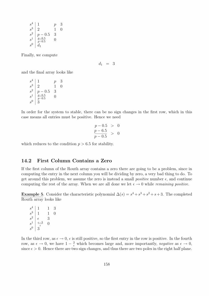
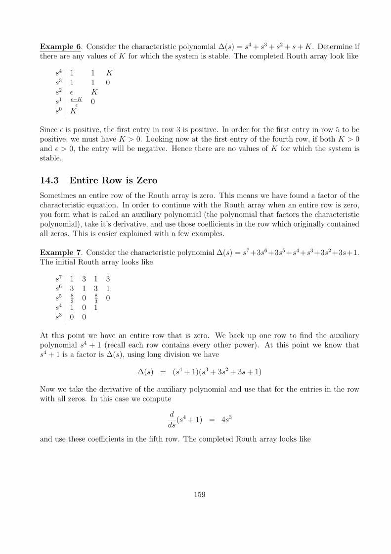
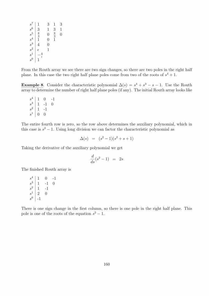
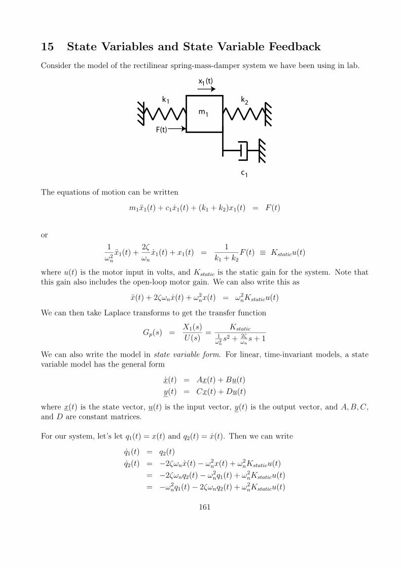
Notes for ECE-320 Fall 2005 by R. Throne The following pages contain a third attempt at writing notes for ECE-320. The topics we cover in ECE-320 are not covered in any single book. These notes are not complete, especially the sections on design using Bode plots. The major sources for these notes are • Analog and Digital Control System Design, by C. T. Chen. Sanders College Publishing. 1993. • Linear Control Systems, by Rohrs, Melsa, and Schulz. McGraw-Hill, 1993. • Modern Control Engineering, by Ogata. Prentice-Hall, 2002. • Modern Control Systems, by Dorf and Bishop. Prentice-Hall, 2005. 1
Transcript
Notes for ECE-320
Fall 2005
byR. Throne
The following pages contain a third attempt at writing notes for ECE-320. The topics we coverin ECE-320 are not covered in any single book. These notes are not complete, especially thesections on design using Bode plots.
The major sources for these notes are
• Analog and Digital Control System Design, by C. T. Chen. Sanders College Publishing.1993.
• Linear Control Systems, by Rohrs, Melsa, and Schulz. McGraw-Hill, 1993.
• Modern Control Engineering, by Ogata. Prentice-Hall, 2002.
• Modern Control Systems, by Dorf and Bishop. Prentice-Hall, 2005.
In this course we will be using Laplace transforms extensively. Although we do not often gofrom the s-plane to the time domain, it is important to be able to do this and to understandwhat is going on. In what follows is a brief review of some results with Laplace transforms.
2.1 Poles and Zeros
Assume we have the transfer function
H(s) =N(s)
D(s)
where N(s) and D(s) are polynomials in s with no common factors. The roots of N(s) are thezeros of the system, while the roots of D(s) are the poles of the system.
2.2 Proper and Strictly Proper Transfer Functions
The transfer function
H(s) =N(s)
D(s)
is proper if the degree of the polynomial N(s) is less than or equal to the degree of the poly-nomial D(s). The transfer function H(s) is strictly proper if the degree of N(s) is less thanthe degree of D(s).
2.3 Impulse Response and Transfer Functions
If H(s) is a transfer function, the inverse Laplace transform of H(s) is call the impulse response,h(t).
L{h(t)} = H(s)
h(t) = L−1{H(s)}
6
2.4 Partial Fractions with Distinct Poles
Let’s assume we have a transfer function
H(s) =N(s)
D(S)=
N(s)
D(s)=
K(s + z1)(s + z2)...(s + zm)
(s + p1)(s + p2)...(s + pn)
where we assume m < n (this makes H(s) a strictly proper transfer function). The poles ofthe system are at −p1, −p2, ... − pn and the zeros of the system are at −z1, −z2, ... − zm.Since we have distinct poles, pi 6= pj for all i and j. Also, since we assumed N(s) and D(s) haveno common factors, we know that zi 6= pj for all i and j.We would like to find the corresponding impulse response, h(t). To do this, we assume
H(s) =N(s)
D(s)= a1
1
s + p1
+ a21
s + p2
+ ... + an1
s + pn
If we can find the ai, it will be easy to determine h(t) since the only inverse Laplace transformwe need is that of 1
s+p, and we know (or can look up) 1
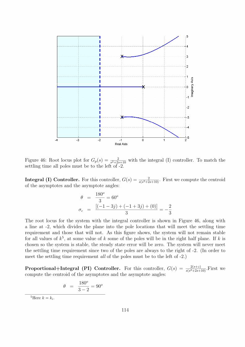
s+p↔ e−ptu(t). To find a1, we first
multiply by (s + p1),
(s + p1)H(s) = a1 + a2s + p1
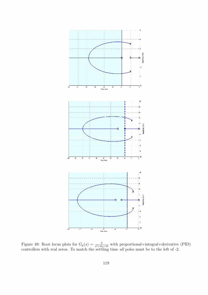
s + p2
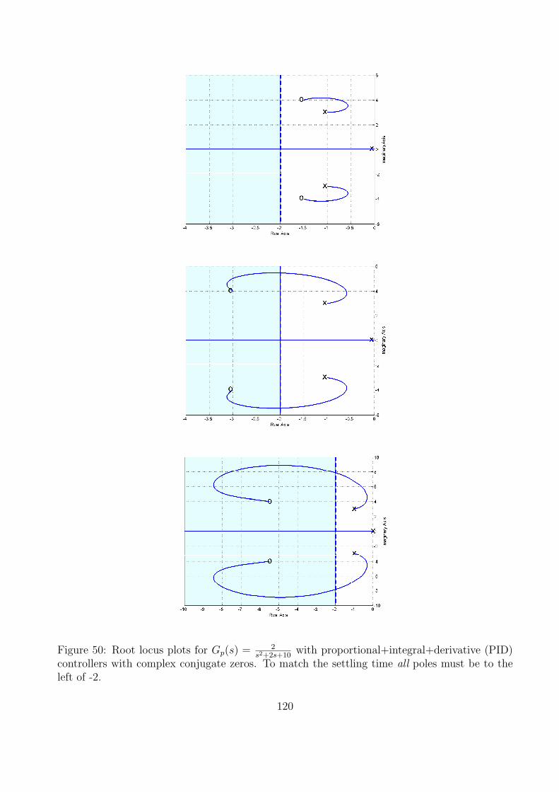
+ ... + ans + p1
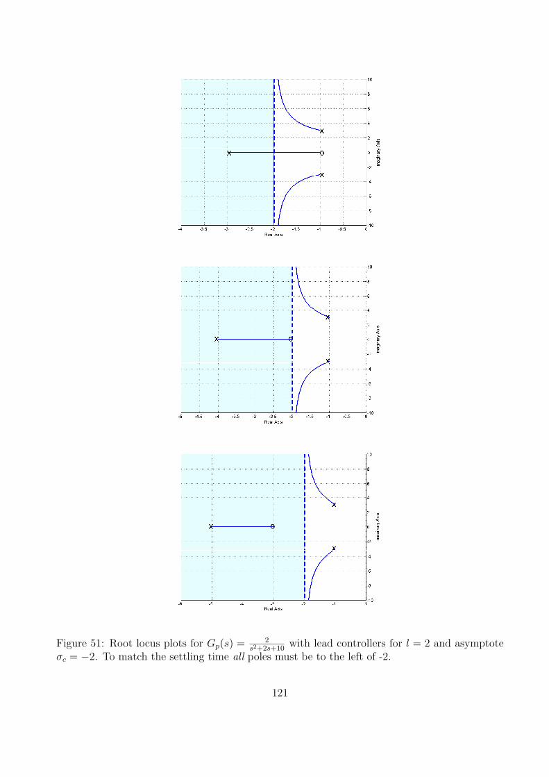
s + pn
and then let s → −p1. Since the poles are all distinct, we will get
lims→−p1
(s + p1)H(s) = a1
Similarly, we will get
lims→−p2
(s + p2)H(s) = a2
and in general
lims→−pi
(s + pi)H(s) = ai
Example 1. Let’s assume we have
H(s) =s + 1
(s + 2)(s + 3)
and we want to determine h(t). Since the poles are distinct, we have
H(s) =(s + 1)
(s + 2)(s + 3)= a1
1
s + 2+ a2
1
s + 3
Then
a1 = lims→−2
(s + 2)(s + 1)
(s + 2)(s + 3)= lim
s→−2
(s + 1)
(s + 3)=−1
1= −1
7
and
a2 = lims→−3
(s + 3)(s + 1)
(s + 2)(s + 3)= lim
s→−3
(s + 1)
(s + 2)=−2
−1= 2
Then
H(s) = −11
s + 2+ 2
1
s + 3
and hence
h(t) = −e−2tu(t) + 2e−3tu(t)
It is often unnecessary to write out all of the steps in the above example. In particular, whenwe want to find ai we will always have a cancellation between (s + pi) in the numerator withthe (s + pi) in the denominator. Using this fact, when we want to find ai we can just ignore (orcover up) the factor (s + pi) in the denominator. For our example above, we then have
a1 = lims→−2
(s + 1)
(s + 3)=−1
1= −1
a2 = lims→−3
(s + 1)
(s + 2)=−2
−1= 2
where we have covered up the poles associated with a1 and a2, respectively.
Example 2. Let’s assume we have
H(s) =s2 − s + 2
(s + 2)(s + 3)(s + 4)
and we want to determine h(t). Since the poles are distinct, we have
H(s) =(s2 − s + 2)
(s + 2)(s + 3)(s + 4)= a1
1
s + 2+ a2
1
s + 3+ a3
1
s + 4
Using the cover up method, we then determine
a1 = lims→−2
(s2 − s + 2)
(s + 3)(s + 4)=
8
(1)(2)= 4
a2 = lims→−3
(s2 − s + 2)
(s + 2) (s + 4)=
14
(−1)(1)= −14
a3 = lims→−4
(s2 − s + 2)
(s + 2)(s + 3)=
22
(−2)(−1)= 11
and hence
h(t) = 4e−2tu(t)− 14e−3tu(t) + 11e−4tu(t)
8
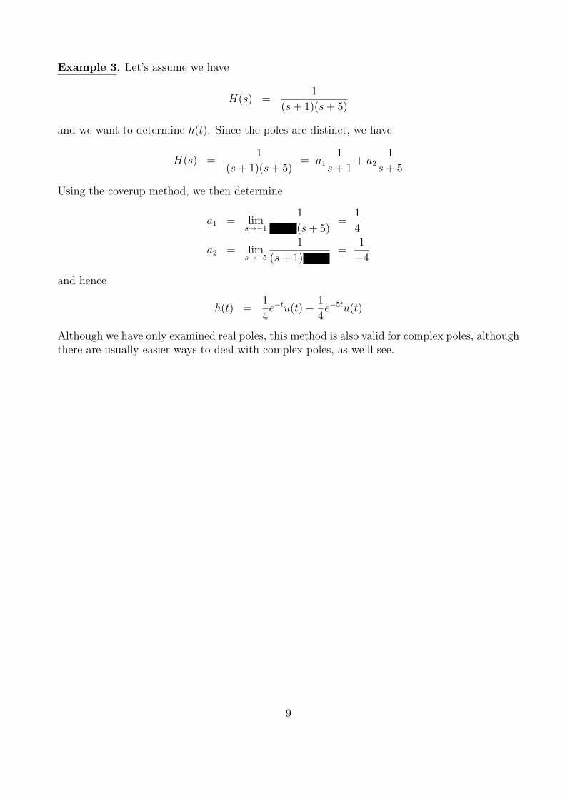
Example 3. Let’s assume we have
H(s) =1
(s + 1)(s + 5)
and we want to determine h(t). Since the poles are distinct, we have
H(s) =1
(s + 1)(s + 5)= a1
1
s + 1+ a2
1
s + 5
Using the coverup method, we then determine
a1 = lims→−1
1
(s + 5)=
1
4
a2 = lims→−5
1
(s + 1)=
1
−4
and hence
h(t) =1
4e−tu(t)− 1
4e−5tu(t)
Although we have only examined real poles, this method is also valid for complex poles, althoughthere are usually easier ways to deal with complex poles, as we’ll see.
9
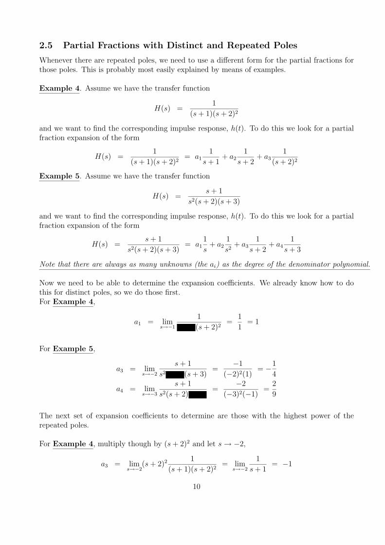
2.5 Partial Fractions with Distinct and Repeated Poles
Whenever there are repeated poles, we need to use a different form for the partial fractions forthose poles. This is probably most easily explained by means of examples.
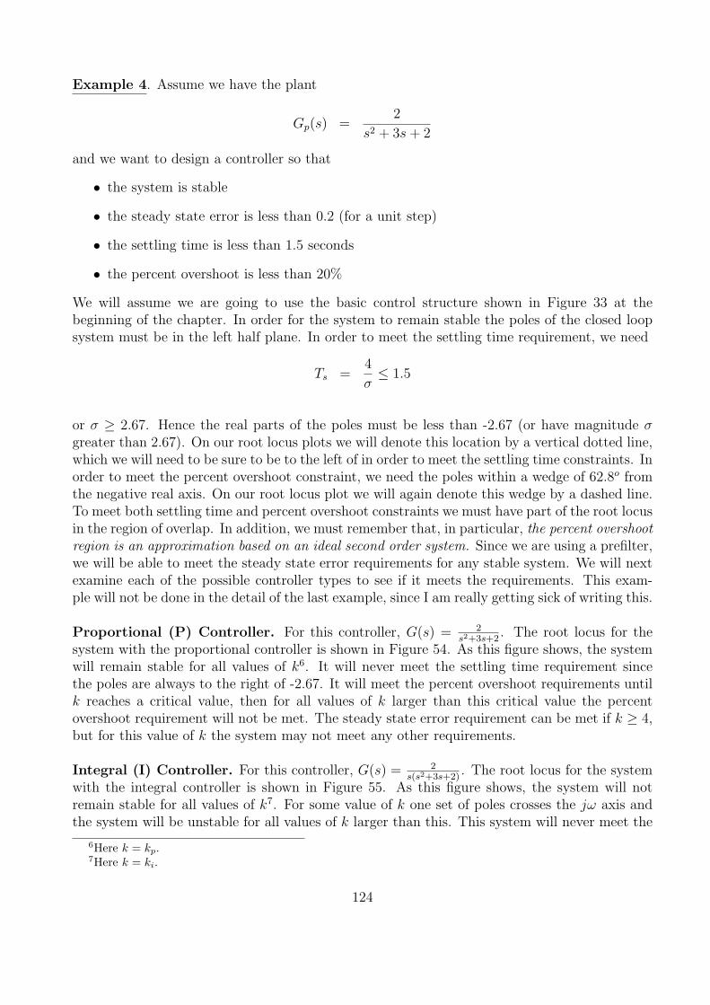
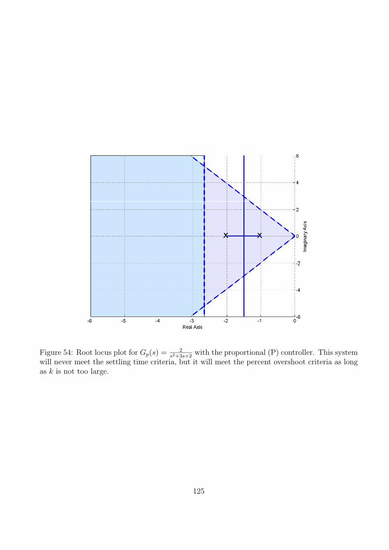
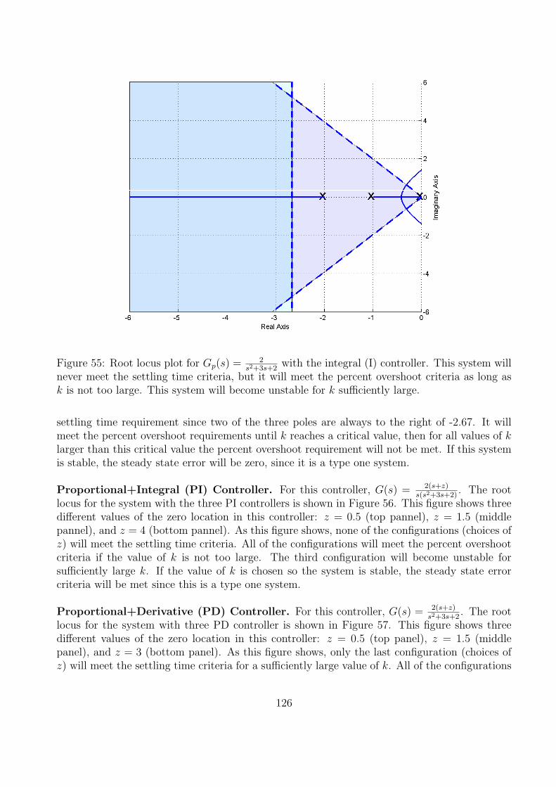
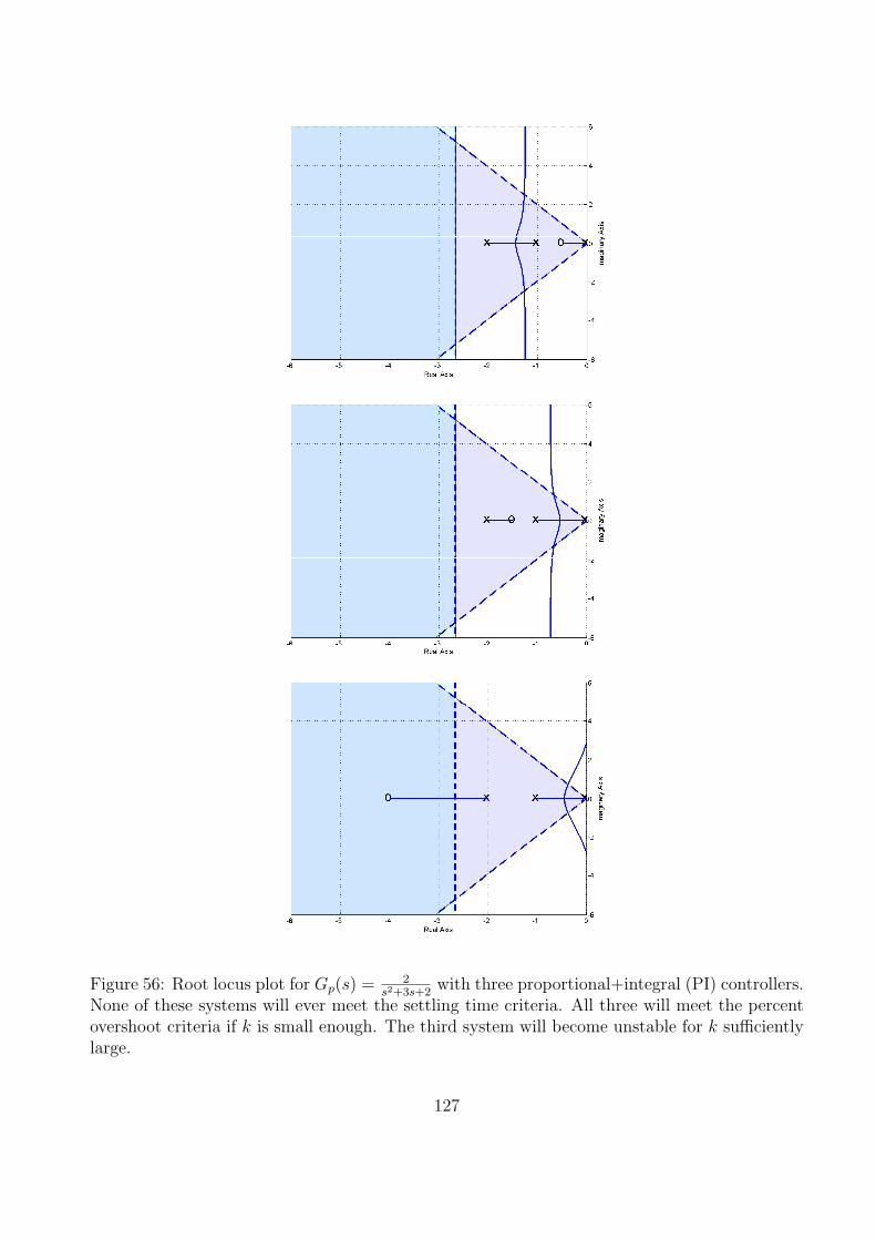
Example 4. Assume we have the transfer function
H(s) =1
(s + 1)(s + 2)2
and we want to find the corresponding impulse response, h(t). To do this we look for a partialfraction expansion of the form
H(s) =1
(s + 1)(s + 2)2= a1
1
s + 1+ a2
1
s + 2+ a3
1
(s + 2)2
Example 5. Assume we have the transfer function
H(s) =s + 1
s2(s + 2)(s + 3)
and we want to find the corresponding impulse response, h(t). To do this we look for a partialfraction expansion of the form
H(s) =s + 1
s2(s + 2)(s + 3)= a1
1
s+ a2
1
s2+ a3
1
s + 2+ a4
1
s + 3
Note that there are always as many unknowns (the ai) as the degree of the denominator polynomial.
Now we need to be able to determine the expansion coefficients. We already know how to dothis for distinct poles, so we do those first.For Example 4,
a1 = lims→−1
1
(s + 2)2=
1
1= 1
For Example 5,
a3 = lims→−2
s + 1
s2 (s + 3)=
−1
(−2)2(1)= −1
4
a4 = lims→−3
s + 1
s2(s + 2)=
−2
(−3)2(−1)=
2
9
The next set of expansion coefficients to determine are those with the highest power of therepeated poles.
For Example 4, multiply though by (s + 2)2 and let s → −2,
a3 = lims→−2
(s + 2)2 1
(s + 1)(s + 2)2= lim
s→−2
1
s + 1= −1
10
or with the coverup method
a3 = lims→−2
1
(s + 1)=
1
−1= −1
For Example 5, multiply though by s2 and let s → 0
a2 = lims→0
s2 s + 1
s2(s + 2)(s + 3)= lim
s→0
s + 1
(s + 2)(s + 3)=
1
6
or with the coverup method
a2 = lims→0
s + 1
(s + 2)(s + 3)=
1
6=
1
6
So far we have:
for Example 4
1
(s + 1)(s + 2)2=
1
s + 1+ a2
1
s + 2− 1
(s + 2)2
and for Example 5
s + 1
s2(s + 2)(s + 3)= a1
1
s+
1
6
1
s2− 1
4
1
s + 2+
2
9
1
s + 3
We now need to determine any remaining coefficients. There are two common ways of doingthis, both of which are based on the fact that both sides of the equation must be equal for anyvalue of s. The two methods are
1. Multiply both sides of the equation by s and let s → ∞. If this works it is usually veryquick.
2. Select convenient values of s and evaluate both sides of the equation for these values of s
For Example 4, using Method 1,
lims→∞
[s
1
(s + 1)(s + 2)2
]= lim
s→∞
[s
s + 1+ a2
s
s + 2− s
(s + 2)2
]
or
0 = 1 + a2 + 0
so a2 = -1.
For Example 5, using Method 1,
lims→∞
[s
s + 1
s2(s + 2)(s + 3)
]= lim
s→∞
[a1
s
s+
1
6
s
s2− 1
4
s
s + 2+
2
9
s
s + 3
]
11
or
0 = a1 + 0− 1
4+
2
9
so a1 = 14− 2
9= 1
36
For Example 4, using Method 2, let’s choose s = 0 (note both sides of the equation must befinite!)
lims→0
[1
(s + 1)(s + 2)2
]= lim
s→0
[1
s + 1+ a2
1
s + 2− 1
(s + 2)2
]
or
1
4= 1 +
a2
2− 1
4
so a2 = 2(14
+ 14− 1) = −1
For Example 5, using Method 2, let’s choose s = −1 (note that s = 0, s = −2, or s = −3 willnot work)
lims→−1
[s + 1
s2(s + 2)(s + 3)
]= lim
s→−1
[a1
1
s+
1
6
1
s2− 1
4
1
s + 2+
2
9
1
s + 3
]
or
0 = −a1 +1
6− 1
4
1
9
so a1 = 16− 1
4+ 1
9= 1
36
Then for Example 4,
h(t) = e−tu(t)− e−2tu(t)− te−2tu(t)
and for Example 5
h(t) =1
36u(t) +
1
6tu(t)− 1
4e−2tu(t) +
2
9e−3tu(t)
In summary, for repeated and distinct poles, go through the following steps:
1. Determine the form of the partial fraction expansion. There must be as many unknownsas the highest power of s in the denominator.
2. Determine the coefficients associated with the distinct poles using the coverup method.
3. Determine the coefficient associated with the highest power of a repeated pole using thecoverup method.
12
4. Determine the remaining coefficients by
• Multiplying both sides by s and letting s →∞• Setting s to a convenient value in both sides of the equations. Both sides must remain
finite
Example 6. Assuming
H(s) =s2
(s + 1)2(s + 3)
determine the corresponding impulse response h(t).
First, we determine the correct form
H(s) =s2
(s + 1)2(s + 3)= a1
1
s + 1+ a2
1
(s + 1)2+ a3
1
s + 3
Second, we determine the coefficient(s) of the distinct pole(s)
a3 = lims→−3
(s2)
(s + 1)2=
9
4
Third, we determine the coefficient(s) of the highest power of the repeated pole(s)
a2 = lims→−1
(s2)
(s + 3)=
1
2
Fourth, we determine any remaining coefficients
lims→∞
[s
s2
(s + 1)2(s + 3)
]= lim
s→∞
[a1
s
s + 1+
1
2
s
(s + 1)2+
9
4
s
(s + 3)
]
or
1 = a1 + 0 +9
4
or a1 = 1− 94
= −54.
Putting it all together, we have
h(t) = −5
4e−tu(t) +
1
2te−tu(t) +
9
4e−3tu(t)
Example 7. Assume we have the transfer function
H(s) =s + 3
s(s + 1)2(s + 2)2
find the corresponding impulse response, h(t).
13
First we determine the correct form
H(s) =s + 3
s(s + 1)2(s + 2)2= a1
1
s+ a2
1
s + 1+ a3
1
(s + 1)2+ a4
1
s + 2+ a5
1
(s + 2)2
Second, we determine the coefficient(s) of the distinct pole(s)
a1 = lims→0
s + 3
(s + 1)2(s + 2)2=
3
(1)(4)=
3
4
Third, we determine the coefficient(s) of the highest power of the repeated pole(s)
a3 = lims→−1
s + 3
s (s + 2)2=
2
(−1)(1)= −2
a5 = lims→−2
s + 3
s(s + 1)2=
1
(−2)(1)= −1
2
Fourth, we determine any remaining coefficients
lims→∞
[s
s + 3
s(s + 1)2(s + 2)2
]= lim
s→∞
[3
4
s
s+ a2
s
s + 1− 2
s
(s + 1)2+ a4
s
s + 2− 1
2
s
(s + 2)2
]
or
0 =3
4+ a2 + a4
We need one more equation, so let’s set s = −3
lims→−3
[s + 3
s(s + 1)2(s + 2)2
]= lim
s→−3
[3
8
1
s+ a2
1
s + 1− 2
1
(s + 1)2+ a4
1
s + 2− 1
2
1
(s + 2)2
]
or
0 = −1
4− a2
1
2− 1
2− a4 − 1
2
This gives us the set of equations
[1 112−1
] [a2
a4
]=
[ −3454
]
with solution a2 = 1 and a4 = −74. Putting it all together we have
h(t) =3
4u(t) + e−tu(t)− 2te−tu(t) +
−7
4e−2tu(t)− 1
2te−2tu(t)
14
2.6 Complex Conjugate Poles: Completing the Square
Before using partial fractions on systems with complex conjugate poles, we need to review oneproperty of Laplace transforms:
if x(t) ⇔ X(s), then e−atx(t) ⇔ X(s + a)
To show this, we start with what we are given:
L{x(t)} =∫ ∞
0x(t)e−stdt = X(s)
Then
L{e−atx(t)} =∫ ∞
0e−atx(t)e−stdt =
∫ ∞
0x(t)e−(s+a)tdt = X(s + a)
The other relationships we need are the Laplace transform pairs for sines and cosines
cos(bt)u(t) ⇔ s
s2 + b2
sin(bt)u(t) ⇔ b
s2 + b2
Finally, we need to put these together, to get the Laplace transform pair:
e−at cos(bt)u(t) ⇔ s + a
(s + a)2 + b2
e−at sin(bt)u(t) ⇔ b
(s + a)2 + b2
Complex poles always result in sines and cosines. We will be trying to make terms with complexpoles look like these terms by completing the square in the denominator.
In order to get the denominators in the correct form when we have complex poles, we need tocomplete the square in the denominator. That is, we need to be able to write the denominatoras
D(s) = (s + a)2 + b2
To do this, we always first find a using the fact that the coefficient of s will be 2a. Then we usewhatever is needed to construct b. A few example will hopefully make this clear.
Example 8. Let’s assume
D(s) = s2 + s + 2
and we want to write this in the correct form. First we recognize that the coefficient of s is 1,so we know 2a = 1 or a = 1
2. We then have
D(s) = s2 + s + 2 = (s +1
2)2 + b2
15
To find b we expand the right hand side of the above equations and then equate powers of s:
D(s) = s2 + s + 2 = (s +1
2)2 + b2 = s2 + s +
1
4+ b2
clearly 2 = b2 + 14, or b2 = 7
4, or b =
√7
2. Hence we have
D(s) = s2 + s + 2 = (s +1
2)2 +
(√7
2
)2
and this is the form we need.
Example 9. Let’s assume
D(s) = s2 + 3s + 5
and we want to write this in the correct form. First we recognize that the coefficient of s is 3,so we know 2a = 3 or a = 3
2. We then have
D(s) = s2 + 3s + 5 = (s +3
2)2 + b2
To find b we expand the right hand side of the above equations and then equate powers of s:
D(s) = s2 + 3s + 5 = (s +3
2)2 + b2 = s2 + 3s +
9
4+ b2
clearly 5 = b2 + 94, or b2 = 11
4, or b =
√112
. Hence we have
D(s) = s2 + 3s + 5 = (s +3
2)2 +
(√11
2
)2
and this is the form we need.
Now that we know how to complete the square in the denominator, we are ready to look atcomplex poles. We will start with two simple examples, and then explain how to deal with morecomplicated examples.
Example 10. Assuming
H(s) =1
s2 + s + 2
and we want to find the corresponding impulse response h(t). In this simple case, we firstcomplete the square, as we have done above, to write
H(s) =1
(s + 12)2 +
(√7
2
)2
16
This almost has the form we want, which is
e−at sin(bt)u(t) ⇔ b
(s + a)2 + b2
However, to use this form we need b in the numerator. To achieve this we will multiply anddivide by b =
√7
2
H(s) =1
(s + 12)2 +
(√7
2
)2
=1√
72
√7
2
(s + 12)2 +
(√7
2
)2
or
h(t) =2√7e−
12t sin(
√7
2t)u(t)
Example 11. Assuming
H(s) =s
s2 + 3s + 5
and we want to find the corresponding impulse response h(t). In this simple case, we firstcomplete the square, as we have done above, to write
H(s) =s
(s + 32)2 +
(√112
)2
This almost has the form we want, which is
e−at cos(bt)u(t) ⇔ (s + a)
(s + a)2 + b2
However, to use this form we need s + a in the numerator, not just s To achieve this we willadd and subtract a = 3
2in the numerator
H(s) =s + 3
2− 3
2
(s + 32)2 +
(√112
)2
=s + 3
2
(s + 32)2 +
(√112
)2 −32
(s + 32)2 +
(√112
)2
The first term is now what we want, and will produce a term of the form
e−32t cos(
√11
2t)u(t)
17
The second term needs some work. It looks like a sine times a decaying exponential, but thescaling is wrong. Again, to put this term in the correct form we will multiply and divide by
√112
H(s) =s + 3
2
(s + 12)2 +
(√112
)2 −3
2
1√
112
√112
(s + 12)2 +
(√112
)2
which gives
h(t) = e−32t cos(
√11
2t)u(t)− 3√
11e−
32t sin(
√11
2t)u(t)
Note that it is possible to combine the sine and cosine terms into a single cosine with a phaseangle, but we will not pursue that here.
The examples we have done so far only contain complex roots. In general, we need to be ableto deal with systems that have both complex and real roots. Since we are dealing with realsystems in this course, all complex poles will occur in complex conjugate pairs. Hence, when wehave complex poles, we will look for quadratic factors of the general form
cs + d
s2 + +es + d
Note that there are two unknown coefficients in this term. Since we need as many unknownsas the highest power of s in the denominator, and this term has 2 powers of s, we need twounknowns. We are now ready to do one more example.
Example 12. Assuming
H(s) =1
(s + 2)(s2 + s + 1)
and we want to determine the corresponding impulse response h(t). First we need to find thecorrect form for the partial fractions
H(s) =1
(s + 2)(s2 + s + 1)= a1
1
s + 2+
a2s + a3
s2 + s + 1
Note that we have three unknowns since the highest power of s in the denominator is 3. Sincethere is an isolated pole at -2, we find coefficient a1 first using the coverup method
a1 = lims→−2
1
(s2 + s + 1)=
1
(−2)2 + (−2) + 1=
1
3
To find a2, let’s use our trick of multiplying by s and letting s →∞
lims→∞
[s
1
(s + 2)(s2 + s + 1)
]= lim
s→∞
[1
3
s
s + 2+
a2s2 + a3s
s2 + s + 1
]
18
or
0 =1
3+ a2
so a2 = −13. Now we have to find a3 and the only trick we have left is choosing a value of s. For
this particular transfer function, s = 0 is a good choice
lims→0
[1
(s + 2)(s2 + s + 1)
]= lim
s→0
[1
3
1
s + 2+
a2s + a3
s2 + s + 1
]
or
1
2=
1
6+ a3
or a3 = 13. So far we have
H(s) =1
3
1
s + 2+
−13s + 1
3
s2 + s + 1
The first term is easy, now we need to work on the second term. First we complete the squarein the denominator
s2 + s + 1 = (s +1
2)2 +
(√3
2
)2
so we have
H(s) =1
3
1
s + 2+
−13s + 1
3
(s + 12)2 +
(√3
2
)2
The next thing to do is to add and subtract 12, so the numerator has the correct form so we have
H(s) =1
3
1
s + 2+−1
3(s + 1
2− 1
2) + 1
3
(s + 12)2 +
(√3
2
)2
=1
3
1
s + 2+−1
3(s + 1
2) + (1
6+ 1
3)
(s + 12)2 +
(√3
2
)2
=1
3
1
s + 2+
−13(s + 1
2) + 1
2
(s + 12)2 +
(√3
2
)2
=1
3
1
s + 2− 1
3
(s + 12)
(s + 12)2 +
(√3
2
)2 +1
2
1
(s + 12)2 +
(√3
2
)2
Finally, we have to scale the final term to put it into the correct form
H(s) =1
3
1
s + 2− 1
3
(s + 12)
(s + 12)2 +
(√3
2
)2 +1
2
1√
32
√3
2
(s + 12)2 +
(√3
2
)2
=1
3
1
s + 2− 1
3
(s + 12)
(s + 12)2 +
(√3
2
)2 +1√3
√3
2
(s + 12)2 +
(√3
2
)2
19
So we finally have
h(t) =1
3e−2tu(t)− 1
3e−
12t cos(
√3
2t)u(t) +
1√3e−
12t sin(
√3
2t)u(t)
2.7 Common Denominator/Cross Multiplying
As a last method, we’ll look at a method of doing partial fractions based on using a common de-nominator. This method is particularly useful for simple problems like finding the step responseof a second order system. However, for many other types of problems it is not very useful, sinceit generates a system of equations that must be solved, much like substituting values of s willdo.Example 13 Let’s assume we have the second order system
H(s) =b
s2 + cs + d
and we want to find the step response of this system,
Y (s) = H(s)1
s
=b
s(s2 + bs + c)= a1
1
s+
a2s + a3
s2 + bs + c
=b
s(s2 + bs + c)=
a1(s2 + bs + c) + s(a2s + a3)
s(s2 + bs + c)
=b
s(s2 + bs + c)=
(a1c)s0 + (a1b + a3)s
1 + (a1 + a2)s2
s(s2 + bs + c)
Since we have made the denominator common for both sides, we just need to equate powers ofs in the numerator:
a1c = b
a1b + a3 = 0
a1 + a2 = 0
Since c and b are known, we can easily solve for a1 in the first equation, then a2 and a3 in theremaining equations.
Example 14. Find the step response of
H(s) =1
s2 + 2s + 2
using the common denominator method. Y (s) is given by
Y (s) =1
s
1
s2 + 2s + 2= a1
1
s+
a2s + a3
s2 + 2s + 2
20
If we put everything over a common denominator we will have the equation
1 = a1(s2 + 2s + 2) + s(a2s + a3)
= (2a1)s0 + (2a1 + a3)s
1 + (a1 + a2)s2
Equating powers of s we get a1 = 12, then a3 = −1 and a2 = −1
2. The we have
Y (s) =1
2
1
s+
−12
s− 1
s2 + 2s + 2
=1
2
1
s− 1
2
s + 2
s2 + 2s + 2
=1
2
1
s− 1
2
(s + 1)
(s + 1)2 + 1− 1
2
1
(s + 1)2 + 1
In the time-domain we have then
y(t) =1
2u(t)− 1
2e−t cos(t)u(t)− 1
2e−t sin(t)u(t)
Example 15. Find the step response of
H(s) =3
2s2 + 3s + 3
using the common denominator method. Partial fractions will only work if the denominator ismonic, which means the leading coefficient must be a 1. Hence we rewrite H(s) as
H(s) =32
s2 + 32s + 3
2
Y (s) is then given by
Y (s) =1
s
32
s2 + 32s + 3
2
= a11
s+
a2s + a3
s2 + 32s + 3
2
If we put everything over a common denominator we will have the equation
3
2= a1(s
2 +3
2s +
3
2) + s(a2s + a3)
= (3
2a1)s
0 + (3
2a1 + a3)s
1 + (a1 + a2)s2
Equating powers of s we get a1 = 1, then a2 = −1 and a3 = −32. The we have
Y (s) =1
s+
−s− 32
s2 + 32s + 3
2
=1
s− s + 3
4+ 3
4
s2 + 32s + 3
2
=1
s− (s + 3
4)
(s + 34)2 +
(√1516
)2 −3
4
√16
15
√1516
(s + 34)2 +
(√1516
)
In the time-domain we have then
y(t) = u(t)− e−3t/4 cos(
√15
16t)u(t)− 3√
15e−3t/4 sin(
√15
16t)u(t)
21
2.8 Complex Conjugate Poles-Again
It is very important to understand the basic structure of complex conjugate poles. For a systemwith complex poles at −a±bj, the characteristic equation (denominator of the transfer function)will be
D(s) = [s− (−a + jb)][s− (−a− jb)]
= [s + (a− jb)][s + (a + jb)]
= s2 + [(a− jb) + (a + jb)]s + (a− jb)(a + jb)
= s2 + 2as + a2 + b2
= (s + a)2 + b2
We know that this form leads to terms of the form e−at cos(bt)u(t) and e−at sin(bt)u(t). Hencewe have the general relationship that complex poles at −a ± jb lead to time domain functionsthat
• decay like e−at (the real part determines the decay rate)
• oscillate like cos(bt) or sin(bt) (the imaginary part determines the oscillation frequency)
These relationships, relating the imaginary and real parts of the poles with corresponding timedomain functions, are very important to remember.
22
3 Final Value Theorem and the Static Gain of a System
The final value theorem for Laplace transforms can generally be stated as follows:If Y (s) has all of its poles in the open left half plane, with the possible exception of a single poleat the origin, then
limt→∞ y(t) = lim
s→0sY (s)
provided the limits exists.
Example 1. For y(t) = e−atu(t) with a > 0 we have
limt→∞ y(t) = lim
t→∞ e−at = 0
lims→0
sY (s) = lims→0
s1
s + a= lim
s→0
s
s + a= 0
Example 2. For y(t) = sin(bt)u(t) we have
limt→∞ y(t) = lim
t→∞ sin(bt)
lims→0
sY (s) = lims→0
sb
s2 + b2= lim
s→0
sb
s2 + b2= 0
Clearly limt→∞ y(t) 6= lims sY (s). Why? Because the final value theorem is not valid since Y (s)has two poles on the jω axis.
Example 3. For y(t) = u(t) we have
limt→∞ y(t) = lim
t→∞u(t) = 1
lims→0
sY (s) = lims→0
s1
s= lim
s→0
s
s= 1
Example 4. For y(t) = e−at cos(bt)u(t) with a > 0 we have
limt→∞ y(t) = lim
t→∞ e−at cos(bt)u(t) = 0
lims→0
sY (s) = lims→0
s(s + a)
(s + a)2 + b2= lim
s→0
s(s + a)
(s + a)2 + b2= 0
One of the common ways in which we use the Final Value Theorem is to compute the staticgain of a system. The response of a transfer function G(s) to a step input of amplitude A,
Y (s) = G(s)A
s
If we want the final value of y(t) then we can use the Final Value Theorem
limt→∞ y(t) = lim
s→0sY (s)
23
= lims→0sG(s)A
s= AG(0)
= AKstatic
provided G(0) exists. G(0) is referred to as the gain or static gain of the system. This is a veryconvenient way of determining the static gain of a system. It is important to remember thatthe steady state value of a system is the static gain of a system multiplied by the amplitude ofthe step input.
Example 5. For the transfer function
G(s) =s + 2
s2 + 3s + 1
the static gain is 2, and if the step input has an amplitude of 0.1, the final value will be 0.2.
Example 6. For the transfer function
G(s) =s2 + 1
s3 + 2s2 + 3s + 4
the static gain is 14, and if the step input has an amplitude of 3, the final value will be 0.75.
24
4 Step Response, Ramp Response, and Steady State Er-
rors
In control systems, we are often most interested in the response of a system to the followingtypes of inputs:
• a step
• a ramp
• a sinusoid
Although in reality control systems have to respond to a large number of different inputs, theseare usually good models for the range of input signals a control system is likely to encounter.
4.1 Step Response and Steady State Error
The step response of a system is the response of the system to a step input. In the time domain,we compute the step response as
y(t) = h(t) ? Au(t)
where A is the amplitude of the step and u(t) is the unit step function and ? is the convolutionoperator. In the s domain, we compute the step response as
Y (s) = H(s)A
sy(t) = L−1{Y (s)}
The steady state error, ess, is the difference between the input and the resulting response ast →∞. For a step input of amplitude A we have
ess = limt→∞ [Au(t)− y(t)]
= A− limt→∞ y(t)
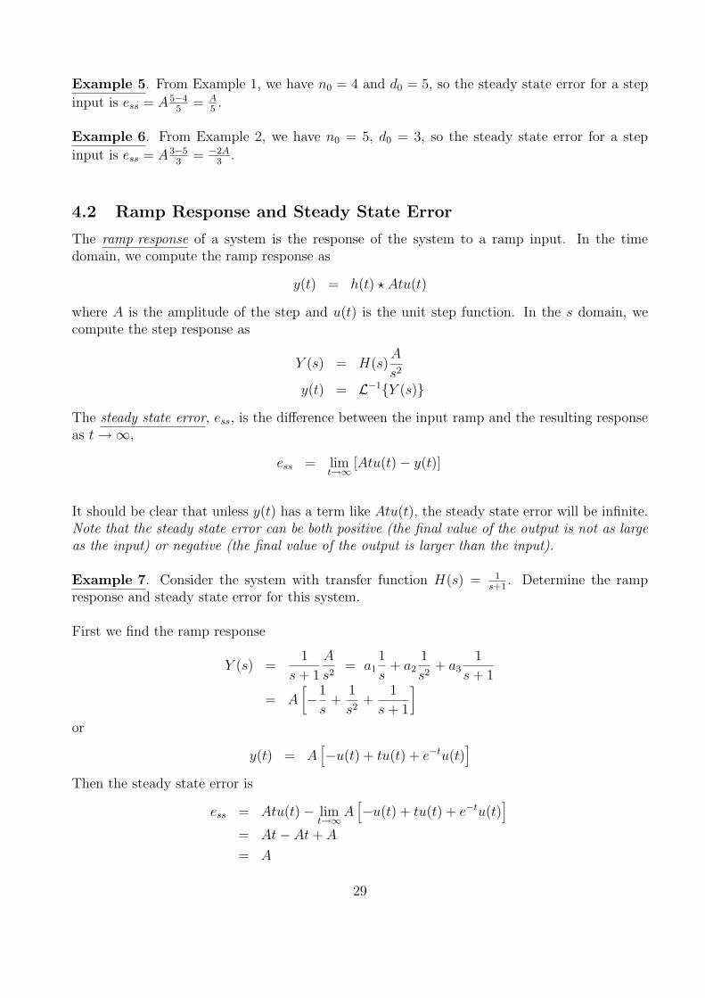
Note that the steady state error can be both positive (the final value of the output is not as largeas the input) or negative (the final value of the output is larger than the input).Example 1. Consider the system with transfer function H(s) = 4
s2+2s+5. Determine step re-
sponse and the steady state error for this system.
First we find the step response,
Y (s) =4
s2 + 2s + 5
A
s= a1
1
s+
a2s + a3
(s + 1)2 + 22
= A
[4
5
1
s−
45s + 8
5
(s + 1)2 + 22
]
= A
[4
5
1
s−
45(s + 1)
(s + 1)2 + 22− 2
5
2
(s + 1)2 + 22
]
25
0 1 2 3 4 5 60
0.2
0.4
0.6
0.8
1
Time (sec)
Dis
plac
emen
t
InputOutput
steady state error = 0.2
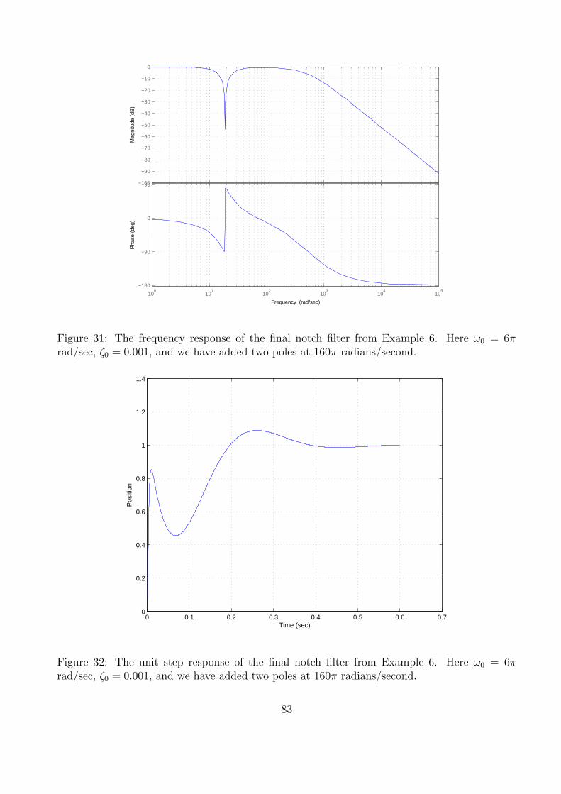
Figure 1: The unit step response and position error for the system in Example 1. This systemhas a positive position error.
or
y(t) = A[4
5u(t)− 4
5e−t cos(2t)u(t)− 2
5e−t sin(2t)u(t)
]
Then the steady state error is
ess = A− limt→∞A
[4
5u(t)− 4
5e−t cos(2t)u(t)− 2
5e−t sin(2t)u(t)
]
= A− 4A
5
=A
5
The step response and steady state error of this system are shown in Figure 1 for a a unit step(A = 1)input. Note that the positive steady state error indicates the final value of the outputis smaller than the final value of the input.
Example 2. Consider the system with transfer function H(s) = 1(s+1)(s+3)
. Determine the stepresponse and steady state error for this system.First we find the step response,
Y (s) =5
(s + 1)(s + 3)
A
s= a1
1
s+ a2
1
s + 1+ a3
1
s + 3
=5A
3
1
s− 5A
2
1
s + 1+
5A
6
1
s + 3
26
0 1 2 3 4 5 6 7 80
0.2
0.4
0.6
0.8
1
1.2
1.4
1.6
1.8
2
Time (sec)
Dis
plac
emen
t
InputOutput
steady state error = −0.667
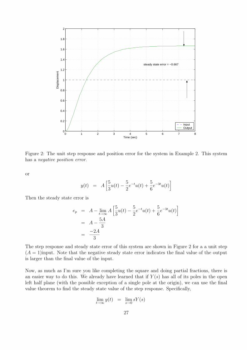
Figure 2: The unit step response and position error for the system in Example 2. This systemhas a negative position error.
or
y(t) = A[5
3u(t)− 5
2e−tu(t) +
5
6e−3tu(t)
]
Then the steady state error is
ep = A− limt→∞A
[5
3u(t)− 5
2e−tu(t) +
5
6e−3tu(t)
]
= A− 5A
3
=−2A
3
The step response and steady state error of this system are shown in Figure 2 for a a unit step(A = 1)input. Note that the negative steady state error indicates the final value of the outputis larger than the final value of the input.
Now, as much as I’m sure you like completing the square and doing partial fractions, there isan easier way to do this. We already have learned that if Y (s) has all of its poles in the openleft half plane (with the possible exception of a single pole at the origin), we can use the finalvalue theorem to find the steady state value of the step response. Specifically,
limt→∞ y(t) = lim
s→0sY (s)
27
= lims→0
s[H(s)
A
s
]
= lims→0
AH(s)
= AH(0)
and then, for stable H(s) we can compute the steady state error as
ess = A− AH(0)
where A is the amplitude of the step input. For a unit step response A = 1.
Example 3. From Example 1, we compute
ess = A− AH(0)
= A− A4
5
=A
5
Example 4. From Example 2, we compute
ess = A− AH(0)
= A− A5
3
=−2A
3
There is yet another way to compute the steady state error, which is useful to know. Let’sassume we write the transfer function as
H(s) =nmsm + nm−1s
m−1 + ... + n2s2 + n1s + n0
sn + dn−1sn−1 + ... + d2s2 + d1s + d0
To compute the steady state error for a step input we need to compute
ess = lims→0
A[1−H(s)]
Let’s write 1−H(s) and put it all over a common denominator. Then we have
1−H(s) =(sn + dn−1s
n−1 + ... + d2s2 + d1s + d0)− (nmsm + nm−1s
m−1 + ... + n2s2 + n1s + n0)
sn + dn−1sn−1 + ... + d2s2 + d1s + d0
=... + (d2 − n2)s
2 + (d1 − n1)s + (d0 − n0)
sn + dn−1sn−1 + ... + d2s2 + d1s + d0
Then
ess = lims→0
A[1−H(s)]
= Ad0 − n0
d0
28
Example 5. From Example 1, we have n0 = 4 and d0 = 5, so the steady state error for a step
input is ess = A5−45
= A5.
Example 6. From Example 2, we have n0 = 5, d0 = 3, so the steady state error for a step
input is ess = A3−53
= −2A3
.
4.2 Ramp Response and Steady State Error
The ramp response of a system is the response of the system to a ramp input. In the timedomain, we compute the ramp response as
y(t) = h(t) ? Atu(t)
where A is the amplitude of the step and u(t) is the unit step function. In the s domain, wecompute the step response as
Y (s) = H(s)A
s2
y(t) = L−1{Y (s)}The steady state error, ess, is the difference between the input ramp and the resulting responseas t →∞,
ess = limt→∞ [Atu(t)− y(t)]
It should be clear that unless y(t) has a term like Atu(t), the steady state error will be infinite.Note that the steady state error can be both positive (the final value of the output is not as largeas the input) or negative (the final value of the output is larger than the input).
Example 7. Consider the system with transfer function H(s) = 1s+1
. Determine the rampresponse and steady state error for this system.
First we find the ramp response
Y (s) =1
s + 1
A
s2= a1
1
s+ a2
1
s2+ a3
1
s + 1
= A[−1
s+
1
s2+
1
s + 1
]
or
y(t) = A[−u(t) + tu(t) + e−tu(t)
]
Then the steady state error is
ess = Atu(t)− limt→∞A
[−u(t) + tu(t) + e−tu(t)
]
= At− At + A
= A
29
Example 8. Consider the system with transfer function H(s) = s+2s2+2s+2
. Determine the rampresponse and steady state error for this system.
First we find the ramp response
Y (s) =s + 2
s2 + 2s + 2
A
s2= a1
1
s+ a2
1
s2+
a3s + a4
s2 + 2s + 2
= A
[−1
2
1
s+
1
s2+
1
2
s
(s + 1)2 + 1
]
= A
[−1
2
1
s+
1
s2+
1
2
s + 1
(s + 1)2 + 1− 1
2
1
(s + 1)2 + 1
]
or
y(t) = A[−1
2u(t) + tu(t) +
1
2e−t cos(t)u(t)− 1
2e−t sin(t)u(t)
]
Then the steady state error is
ess = Atu(t)− limt→∞A
[−1
2u(t) + tu(t) +
1
2e−t cos(t)u(t)− 1
2e−t sin(t)u(t)
]
= At− At +1
2A
=A
2
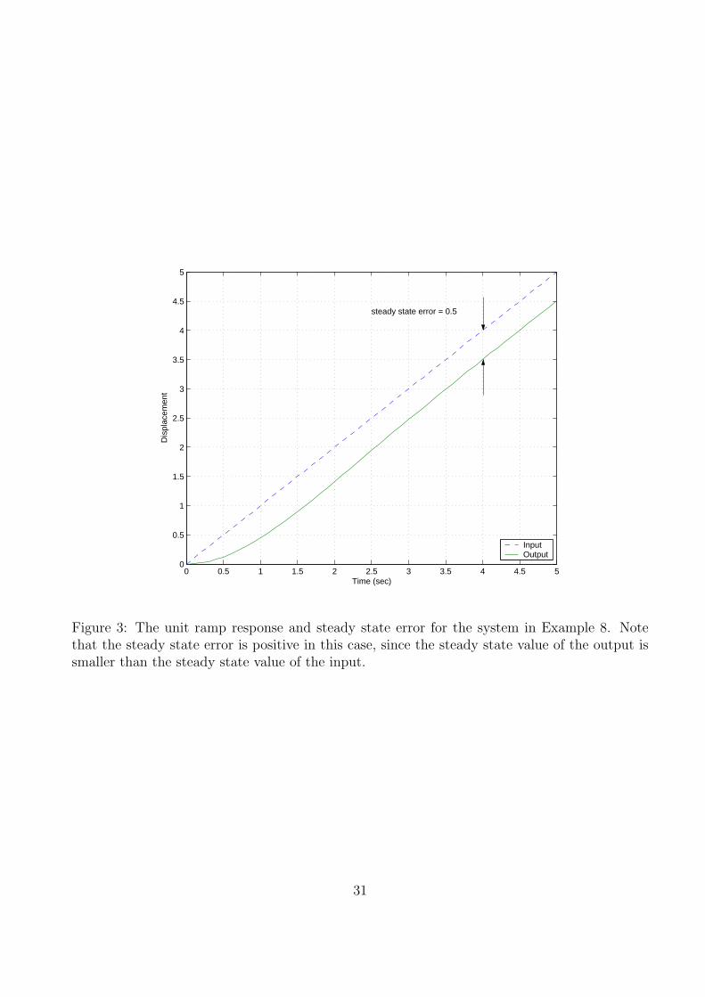
The ramp response and steady state error for this system are shown in Figure 3 for a a unitramp input. Note that the steady state error is positive, indicating the output of the system issmaller than the input in steady state.We can try and use the Final Value Theorem again, but it becomes a bit more complicated. Wewant to find
ess = limt→∞ [Atu(t)− y(t)]
= lims→0
s[A
s2− A
s2H(s)
]
= lims→0
A
s[1−H(s)]
Let’s assume again we can write the transfer function as
H(s) =nmsm + nm−1s
m−1 + ... + n2s2 + n1s + n0
sn + dn−1sn−1 + ... + d2s2 + d1s + d0
If we compute 1−H(s) and put things over a common denominator, we have
1−H(s) =(sn + dn−1s
n−1 + ... + d2s2 + d1s + d0)− (nmsm + nm−1s
m−1 + ... + n2s2 + n1s + n0)
sn + dn−1sn−1 + ... + d2s2 + d1s + d0
=... + (d2 − n2)s
2 + (d1 − n1)s + (d0 − n0)
sn + dn−1sn−1 + ... + d2s2 + d1s + d0
30
0 0.5 1 1.5 2 2.5 3 3.5 4 4.5 50
0.5
1
1.5
2
2.5
3
3.5
4
4.5
5
Time (sec)
Dis
plac
emen
t
InputOutput
steady state error = 0.5
Figure 3: The unit ramp response and steady state error for the system in Example 8. Notethat the steady state error is positive in this case, since the steady state value of the output issmaller than the steady state value of the input.
31
and
1
s[1−H(s)] =
... + (d2 − n2)s+(d1 − n1) + (d0 − n0)
1s
sn + dn−1sn−1 + ... + d2s2 + d1s + d0
Now, in order to have ess be finite, we must get a finite value as s → 0 in this expression. Thevalue of the denominator will be d0 as s → 0, so the denominator will be OK. All of the termsin the numerator will be zero except the last two: (d1− n1) + (d0− n0)
1s
In order to get a finitevalue from these terms, we must have n0 = d0, that is, constant terms in the numerator anddenominator must be the same. This also means that the system must have a zero steady stateerror for a step input. Important!! If the system does not have a zero steady state error for astep input, the steady state error for a ramp input will be infinite! Conversely, if a system hasfinite steady state error for a ramp input, the steady state error for a step input must be zero!If n0 = d0, then we have
ess = lims→0
A
s[1−H(s)] = A
d1 − n1
d0
Example 9. For the system in Example 7, H(s) = 1s+1
. Here n0 = d0 = 1, so the systemhas zero steady state error for a step input, and n1 = 0, d1 = 1. Hence for a ramp inputess = Ad1−n1
d0= A.
Example 10. For the system in Example 8, H(s) = s+2s2+2s+2
. Here n0 = d0 = 2, so the systemhas zero steady state error for a step input, and n1 = 1, d1 = 2. Hence for a ramp inputess = Ad1−n1
d0= A
2.
4.3 Summary
Assume we write the transfer function of a system as
H(s) =nmsm + nm−1s
m−1 + ... + n2s2 + n1s + n0
sn + dn−1sn−1 + ... + d2s2 + d1s + d0
The step response of a system is the response of the system to a step input. The steady stateerror, ess, for a step input is the difference between the input and the output of the system insteady state. We can compute the steady state error for a step input in a variety of ways:
ess = limt→∞ [Au(t)− y(t)]
= A− limt→∞ y(t)
= A(1−H(0))
= Ad0 − n0
d0
The ramp response of a system is the response of the system to a ramp input. The steady stateerror, ess, for a ramp input is the difference between the input and output of the system insteady state. A system has infinite steady state error for a ramp input unless the steady state
32
error for a step input is zero. We can compute the steady state error for a ramp input in avariety of ways:
ess = limt→∞ [At− y(t)]
= Ad1 − n1
d0
33
5 Response of a Ideal Second Order System
This is an important example, which you have probably seen before. Let’s assume we have anideal second order system with transfer function
H(s) =Kstatic
1ωn
2s2 + 2ζ
ωns + 1
=Kstatic ωn
2
s2 + 2ζωns + ω2n
where ζ is the damping ratio, ωn is the natural frequency, and Kstatic is the static gain. Thepoles of the transfer function are the roots of the denominator, which are given by the quadraticformula
roots =−2ζωn ±
√(2ζωn)2 − 4ω2
n
2
= −ζωn ± ωn
√ζ2 − 1
= −ζωn ± jωn
√1− ζ2
= −ζωn ± jωd
= −σ ± jωd
= −1/τ ± jωd
where we have used the damped frequency ωd = ωn
√1− ζ2 and σ = 1
τ= ζωn. As we start to
talk about systems with more than two poles, it is easier to remember to use the form of thepoles −σ ± ωd or −1/τ ± ωd.
5.1 Step Response of an Ideal Second Order System
To find the step response,
Y (s) = H(s)U(s) =Kstatic ω2
n
s2 + 2ζωns + ω2n
1
s
We then look for a partial fraction expansion in the form
Y (s) =Kstatic ω2
n
s2 + 2ζωns + ω2n
1
s= a1
1
s+
a2s + a3
s2 + 2ζωns + ω2n
From this, we can determine that a1 = Kstatic, a2 = −Kstatic, and a3 = −2ζωnKstatic. Hence wehave
Y (s) = Kstatic1
s−Kstatic
s + 2ζωn
s2 + 2ζωns + ω2n
Completing the square in the denominator we have
Y (s) = Kstatic1
s−Kstatic
s + 2ζωn
(s + ζωn)2 + ω2d
34
or
Y (s) = Kstatic1
s−Kstatic
s + ζωn
(s + ζωn)2 + ω2d
−Kstaticζωn
(s + ζωn)2 + ω2d
= Kstatic1
s−Kstatic
s + ζωn
(s + ζωn)2 + ω2d
−Kstaticζωn
ωd
ωd
(s + ζωn)2 + ω2d
or in the time domain
y(t) = Kstatic
[1− e−ζωnt cos(ωdt)− ζωn
ωd
e−ζωnt sin(ωdt)
]u(t)
We would now like to write the sine and cosine in terms of a sine and a phase angle. To do this,we use the identity
r sin(ωd + θ) = r cos(ωd) sin(θ) + r sin(ωd) cos(θ)
Hence we have
r sin(θ) = 1
r cos(θ) =ζωn
ωd
=ζ√
1− ζ2
Hence
θ = tan−1
(√1− ζ2
ζ
)
r =1√
1− ζ2
Note that
cos(θ) =ζ√
1− ζ2
1
r=
ζ√1− ζ2
√1− ζ2
or θ = cos−1(ζ). Finally we have
y(t) = Kstatic
[1− 1√
1− ζ2e−ζωnt sin(ωdt + θ)
]u(t)
5.2 Time to Peak, Tp
From our solution of the response of the ideal second order system to a unit step, we can computethe time to peak by taking the derivative of y(t) and setting it equal to zero. This will give usthe maximum value of y(t) and the time that this occurs at is called the time to peak, Tp.
dy(t)
dt= − Kstatic√
1− ζ2
[−ζωne
−ζωnt sin(ωdt + θ) + ωde−ζωnt cos(ωdt + θ)
]= 0
35
or
ζωn sin(ωdt + θ) = ωd cos(ωdt + θ)
tan(ωdt + θ) =
√1− ζ2
ζ
θ + ωdt = tan−1
(√1− ζ2
ζ
)
but we already have θ = tan−1
(√1−ζ2
ζ
), hence ωdt must be equal to one period of the tangent,
which is π. Hence
Tp =π
ωd
Remember that ωd is equal to the imaginary part of the complex poles.
5.3 Percent Overshoot, PO
Evaluating y(t) at the peak time Tp we get the maximum value of y(t),
y(Tp) = Kstatic
[1− 1√
1− ζ2e−ζωnTp sin(ωdTp + θ)
]
= Kstatic
[1− 1√
1− ζ2e−ζωnπ/ωd sin(ωd
π
ωd
+ θ)
]
= Kstatic
[1 +
1√1− ζ2
e−ζπ/√
1−ζ2sin(θ)
]
since sin(θ + π) = − sin(θ). Then sin(θ) =√
1− ζ2, hence
y(t) = Kstatic
[1 + e
− ζπ√1−ζ2
]
The percent overshoot is defined as
Percent Overshoot = P.O. =y(Tp)− y(∞)
y(∞)× 100%
For our second order system we have y(∞) = Kstatic, so
P.O. =Kstatic
[1 + e
− ζπ√1−ζ2
]−Kstatic
Kstatic
× 100%
or
P.O. = e− ζπ√
1−ζ2 × 100%
36
5.4 Settling Time, Ts
The settling time is defined as the time it takes for the output of a system with a step inputto stay within a given percentage of its final value. In this course, we use the 2% settling timecriteria, which is generally four time constants. For any exponential decay, the general form iswritten as e−t/τ , where τ is the time constant. For the ideal second order system response, wehave τ = 1/ζωn or σ = ζωn. Hence, for and ideal second order system, we estimate the settlingtime as
Ts = 4τ =4
σ=
4
ζωn
For systems other than second order systems we will want to talk about the settling time, hencethe use of the forms
Ts = 4τ =4
σ
are often more appropriate to remember.
Example 1. Consider the system with transfer function given by
H(s) =9
s2 + βs + 9
determine the range of β so that Ts ≤ 5 seconds and Tp ≤ 1.2 seconds.
For the transfer function, we see that ωn = 3 and 2ζωn = β, so ζ = β/(2ωn) = β/6. For thesettling time constraint we have
Ts =4
ζωn
≤ 5
4β63
≤ 5
8
5≤ β
so β ≥ 1.60. For the time to peak constraint, we have
Tp =π
ωd
≤ 1.2
π
ωn
√1− ζ2
≤ 1.2
π
1.2ωn
≤√
1− ζ2
(π
1.2ωn
)2
≤ 1− ζ2
ζ2 ≤ 1−(
π
1.2ωn
)2
ζ ≤√
1−(
π
1.2ωn
)2
β ≤ 6
√1−
(π
1.2ωn
)2
37
0 0.5 1 1.5 2 2.5 3 3.5 4 4.5 50
0.2
0.4
0.6
0.8
1
1.2
1.4
Time (sec)
Am
plitu
de
Figure 4: Step response for the system H(s) = 9s2+2.265s+9
. The settling time should be less than5 seconds, the time to peak should be less than 1.2 seconds, and the percent overshoot shouldbe 27.8%.
or β ≤ 2.93. To meet both constraints we need 1.60 ≤ β ≤ 2.93. Let’s choose the average,so β = 2.265. Then ζ = 0.3775 and the percent overshoot is 27.8%. The step response of thissystem is shown in Figure 4.
Example 2. Consider the system with transfer function given by
H(s) =K
s2 + 2s + K
determine the range of K so that PO ≤ 20%. Is there any value of K so that Ts ≤ 2 seconds?
For the transfer function, we see that ωn =√
K and 2ζωn = 2, so ζωn = 1 and ζ = 1√K
. For the
percent overshoot we have b = 20/100 = 0.2 and
e− ζπ√
1−ζ2 ≤ b
− ζπ√1− ζ2
≤ ln(b)
− π√K
1√1− 1
K
≤ ln(b)
− π√K − 1
≤ ln(b)
38
0 1 2 3 4 5 60
0.2
0.4
0.6
0.8
1
1.2
1.4
Time (sec)
Am
plitu
de
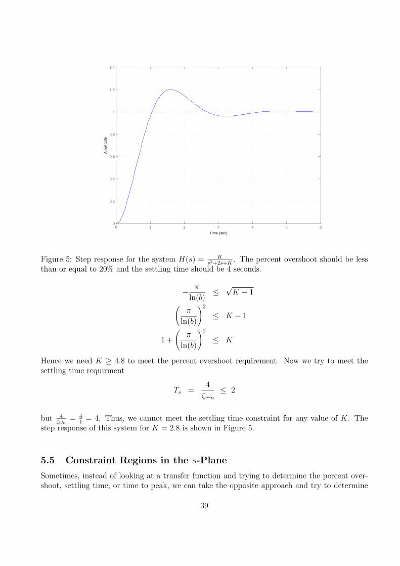
Figure 5: Step response for the system H(s) = Ks2+2s+K
. The percent overshoot should be lessthan or equal to 20% and the settling time should be 4 seconds.
− π
ln(b)≤
√K − 1
(π
ln(b)
)2
≤ K − 1
1 +
(π
ln(b)
)2
≤ K
Hence we need K ≥ 4.8 to meet the percent overshoot requirement. Now we try to meet thesettling time requirment
Ts =4
ζωn
≤ 2
but 4ζωn
= 41
= 4. Thus, we cannot meet the settling time constraint for any value of K. Thestep response of this system for K = 2.8 is shown in Figure 5.
5.5 Constraint Regions in the s-Plane
Sometimes, instead of looking at a transfer function and trying to determine the percent over-shoot, settling time, or time to peak, we can take the opposite approach and try to determine
39
the region in the s-plane the poles of the system should be located in to achieve a given criteria.Each one of the three criteria will determine a region of space in the s-plane.
Time to Peak (Tp) Let’s assume we have a maximum time to peak given, Tmaxp , and we want
to know where to find all of the poles that will meet this constraint. We have
Tp =π
ωd
≤ Tmaxp
we can rearrange this as
π
Tmaxp
≤ ωd
Since we can write the complex poles as −σ ± jωd, this means that the imaginary part of thepoles must be greater than π
T maxp
.
Example 3. Determine all acceptable pole location so that the time to peak will be less than2 seconds. We have Tmax
p = 2, so ωd ≥ π2
= 1.57. The acceptable pole locations are shown inthe shaded region of Figure 6.
Figure 6: Acceptable pole locations for Tp ≤ 2 seconds are shown in the shaded region.
40
Percent Overshoot (P.O.) Let’s assume we have a maximum percent overshoot given, POmax,and we want to know where to find all of the poles that will meet this constraint. We have
P.O. = e− ζπ√
1−ζ2 × 100% ≤ POmax
or
e− ζπ√
1−ζ2 ≤ POmax
100= b
where we have defined the parameter b = POmax/100 for notational convenience. We need tofirst solve the above expression for ζ.
− ζπ√1− ζ2
≤ ln(b)
ζ√1− ζ2
≥ − ln(b)
π
ζ2
1− ζ2≥
(− ln(b)
π
)2
ζ2 ≥(− ln(b)
π
)2
− ζ2
(− ln(b)
π
)2
ζ2
1 +
(− ln(b)
π
)2 ≥
(− ln(b)
π
)2
ζ ≥− ln(b)
π√1 +
(− ln(b)π
)2
Now we use the relationship
θ = cos−1 (ζ)
In summary, we have
θ ≤ cos−1 (ζ) , ζ ≥− ln(b)
π√1 +
(− ln(b)π
)2, b =
POmax
100
This angle θ is measured from the negative real axis. Hence an angle of 90 degrees indicatesζ = 0 and there is no damping (the poles are on the jω axis), while an angle of 0 degrees meansthe system has a damping ratio of 1, and the poles are purely real.
41
Example 4. Determine all acceptable pole locations so that the percent overshoot will be lessthan 10%. We have b = 0.1, so ζ ≥ 0.59 and θ ≤ 53.8o The acceptable pole locations are shownin the shaded region of Figure 7.
Figure 7: Acceptable pole locations for Percent Overshoot less than or equal to 10%. Theacceptable pole locations are shown in the shaded region.
42
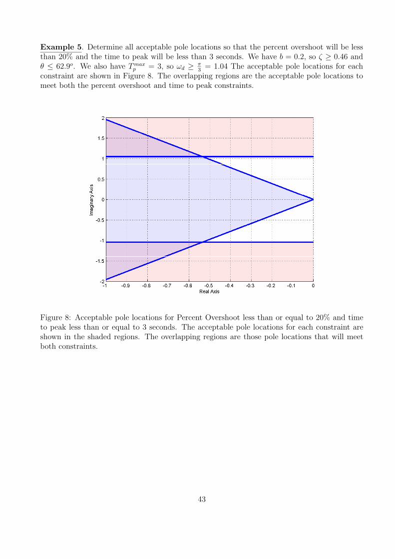
Example 5. Determine all acceptable pole locations so that the percent overshoot will be lessthan 20% and the time to peak will be less than 3 seconds. We have b = 0.2, so ζ ≥ 0.46 andθ ≤ 62.9o. We also have Tmax
p = 3, so ωd ≥ π3
= 1.04 The acceptable pole locations for eachconstraint are shown in Figure 8. The overlapping regions are the acceptable pole locations tomeet both the percent overshoot and time to peak constraints.
Figure 8: Acceptable pole locations for Percent Overshoot less than or equal to 20% and timeto peak less than or equal to 3 seconds. The acceptable pole locations for each constraint areshown in the shaded regions. The overlapping regions are those pole locations that will meetboth constraints.
43
Settling Time (Ts) Let’s assume we have a maximum settling time Tmaxs , and we want to
know where to find all of the poles that will meet this constraint. We have
Ts =4
σ≤ Tmax
s
or
4
Tmaxs
≤ σ
Since we can write the complex poles as −σ ± jωd, this means that the real part of the polesmust be greater (in magnitude) than 4
T maxs
. In other words, the poles must have real parts less
than − 4T max
s
Example 6. Determine all acceptable pole locations so that the settling time will be less than3 seconds. We have Tmax
s = 3, so σ ≥ 4T max
s= 4
3= 1.333. The acceptable pole locations are
shown in Figure 9.
Figure 9: Acceptable pole locations for settling time less than or equal to 3 seconds. Theacceptable pole locations are shown in the shaded region.
44
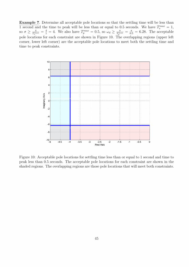
Example 7. Determine all acceptable pole locations so that the settling time will be less than1 second and the time to peak will be less than or equal to 0.5 seconds. We have Tmax
s = 1,so σ ≥ 4
T maxs
= 41
= 4. We also have Tmaxp = 0.5, so ωd ≥ π
T maxp
= π0.5
= 6.28. The acceptable
pole locations for each constraint are shown in Figure 10. The overlapping regions (upper leftcorner, lower left corner) are the acceptable pole locations to meet both the settling time andtime to peak constraints.
Figure 10: Acceptable pole locations for settling time less than or equal to 1 second and time topeak less than 0.5 seconds. The acceptable pole locations for each constraint are shown in theshaded regions. The overlapping regions are those pole locations that will meet both constraints.
45
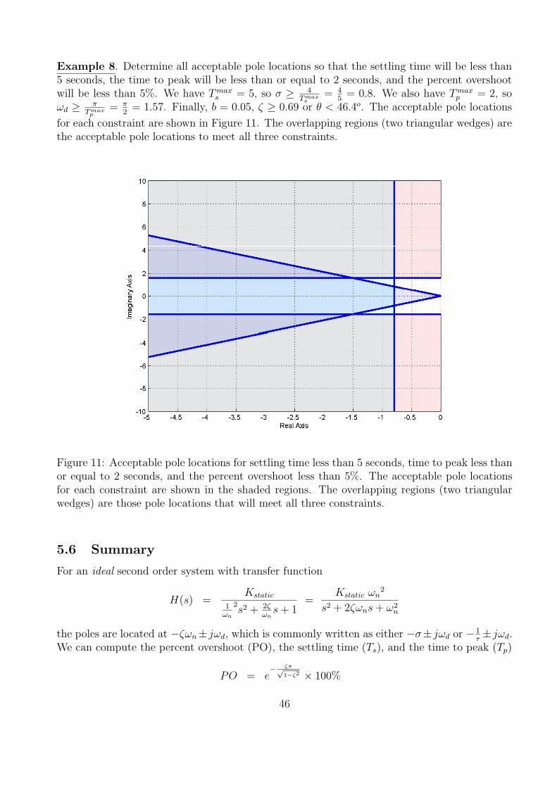
Example 8. Determine all acceptable pole locations so that the settling time will be less than5 seconds, the time to peak will be less than or equal to 2 seconds, and the percent overshootwill be less than 5%. We have Tmax
s = 5, so σ ≥ 4T max
s= 4
5= 0.8. We also have Tmax
p = 2, soωd ≥ π
T maxp
= π2
= 1.57. Finally, b = 0.05, ζ ≥ 0.69 or θ < 46.4o. The acceptable pole locations
for each constraint are shown in Figure 11. The overlapping regions (two triangular wedges) arethe acceptable pole locations to meet all three constraints.
Figure 11: Acceptable pole locations for settling time less than 5 seconds, time to peak less thanor equal to 2 seconds, and the percent overshoot less than 5%. The acceptable pole locationsfor each constraint are shown in the shaded regions. The overlapping regions (two triangularwedges) are those pole locations that will meet all three constraints.
5.6 Summary
For an ideal second order system with transfer function
H(s) =Kstatic
1ωn
2s2 + 2ζ
ωns + 1
=Kstatic ωn
2
s2 + 2ζωns + ω2n
the poles are located at −ζωn± jωd, which is commonly written as either −σ± jωd or − 1τ± jωd.
We can compute the percent overshoot (PO), the settling time (Ts), and the time to peak (Tp)
PO = e− ζπ√
1−ζ2 × 100%
46
Ts =4
ζωn
= 4τ =4
σ
Tp =π
ωd
It is important to remember that these relationships are only valid for ideal second order sys-tems!
What is generally more useful to us is to use these relationships to determine acceptable polelocations to meet the various design criteria. If the maximum desired settling time is Tmax
s , thenall poles must have real parts less than −4/Tmax
s . If the maximum desired time to peak is Tmaxp ,
then the imaginary parts of the dominant poles must have imaginary parts larger than π/Tmaxp ,
or less than −π/Tmaxp (since poles come in complex conjugate pairs). If the maximum percent
overshoot is POmax, then the poles must lie in a wedge determined by θ = cos−1 (ζ) where θ ismeasured from the negative real axis and
ζ ≥− ln(b)
π√1 +
(− ln(b)π
)2, b =
POmax
100
Each of these constraints can be used to define a region of acceptable pole locations for an idealsecond order system. However, they are often used as a guide (or starting point) for higherorder systems, and systems with zeros.
47
6 Characteristic Polynomial, Modes, and Stability
In this section, we first introduce the concepts of the characteristic polynomial, characteristicequation, and characteristic modes. You’ll obviously note the word characteristic is used quitea lot here. Then, we utilize these concepts to define stability of our systems.
6.1 Characteristic Polynomial, Equation, and Modes
Consider a transfer function
H(s) =N(s)
D(s)
where N(s) and D(s) are polynomials in s with no common factors. D(s) is called the character-istic polynomial of the system, and the equation D(s) = 0 is called the characteristic equation.The time functions associated with the roots of the characteristic equation (the poles of thesystem) are called the characteristic modes. To determine the characteristic modes, it is ofteneasiest to think of doing partial fraction expansion and looking at the resulting time functions.Some examples will probably help.
The impulse response is a linear combination of characteristic modes:
h(t) = a1u(t) + a2e−tu(t) + a3te
−tu(t) + a4e−3tu(t)
48
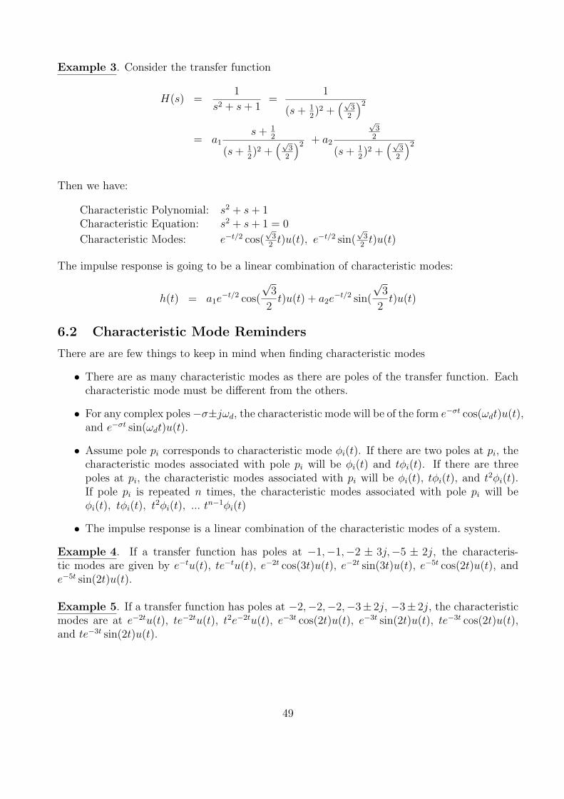
Example 3. Consider the transfer function
H(s) =1
s2 + s + 1=
1
(s + 12)2 +
(√3
2
)2
= a1
s + 12
(s + 12)2 +
(√3
2
)2 + a2
√3
2
(s + 12)2 +
(√3
2
)2
Then we have:
Characteristic Polynomial: s2 + s + 1Characteristic Equation: s2 + s + 1 = 0
Characteristic Modes: e−t/2 cos(√
32
t)u(t), e−t/2 sin(√
32
t)u(t)
The impulse response is going to be a linear combination of characteristic modes:
h(t) = a1e−t/2 cos(
√3
2t)u(t) + a2e
−t/2 sin(
√3
2t)u(t)
6.2 Characteristic Mode Reminders
There are are few things to keep in mind when finding characteristic modes
• There are as many characteristic modes as there are poles of the transfer function. Eachcharacteristic mode must be different from the others.
• For any complex poles−σ±jωd, the characteristic mode will be of the form e−σt cos(ωdt)u(t),and e−σt sin(ωdt)u(t).
• Assume pole pi corresponds to characteristic mode φi(t). If there are two poles at pi, thecharacteristic modes associated with pole pi will be φi(t) and tφi(t). If there are threepoles at pi, the characteristic modes associated with pi will be φi(t), tφi(t), and t2φi(t).If pole pi is repeated n times, the characteristic modes associated with pole pi will beφi(t), tφi(t), t2φi(t), ... tn−1φi(t)
• The impulse response is a linear combination of the characteristic modes of a system.
Example 4. If a transfer function has poles at −1,−1,−2 ± 3j,−5 ± 2j, the characteris-tic modes are given by e−tu(t), te−tu(t), e−2t cos(3t)u(t), e−2t sin(3t)u(t), e−5t cos(2t)u(t), ande−5t sin(2t)u(t).
Example 5. If a transfer function has poles at −2,−2,−2,−3± 2j, −3± 2j, the characteristicmodes are at e−2tu(t), te−2tu(t), t2e−2tu(t), e−3t cos(2t)u(t), e−3t sin(2t)u(t), te−3t cos(2t)u(t),and te−3t sin(2t)u(t).
49
6.3 Stability
A system is defined to be stable if all of its characteristic modes go to zero as t →∞. A systemis defined to be marginally stable if all of its characteristic modes are bounded as t → ∞. Asystem is unstable if any of its characteristic modes is unbounded as t → ∞. There are otherdefinitions of stability, each with their own purpose. For the systems we will be studying in thiscourse, generally linear time invariant systems, these are the most appropriate. Note that thestability of a system is independent of the input.
In determining stability, the following mathematical truths should be remembered
limt→∞ tne−at = 0 for all positive a and n
limt→∞ e−at cos(ωdt + φ) = 0 for all positive a
limt→∞ e−at sin(ωdt + φ) = 0 for all positive a
u(t) is bounded
cos(ωdt + φ) is bounded
sin(ωdt + φ) is bounded
Example 6. Assume a system has poles at −1, 0,−2. Is the system stable?
The characteristic modes of the system are e−tu(t), u(t), and e−2tu(t). Both e−tu(t) and e−2tu(t)go to zero as t →∞. u(t) does not go to zero, but it is bounded. Hence the system is marginallystable.
Example 7. Assume a system has poles at −1, 1,−2± 3j. Is the system stable?
The characteristic modes of the system are e−tu(t), etu(t), e−2t cos(3t)u(t), and e−2t sin(3t). Allof these modes go to zero as t goes to infinity, except the mode etu(t). This mode is unboundedas t →∞. Hence the system is unstable.
Example 8. Assume a system has poles at −1,−1,−2± j,−2± j. Is the system stable?
The characteristic modes of the system are e−tu(t), te−tu(t), e−2t cos(t)u(t), e−2t sin(t)u(t),te−2t cos(t)u(t), and te−2t sin(t)u(t). All of the characteristic modes go to zero as t goes toinfinity, so the system is stable.
6.4 Settling Time and Dominant Poles
For an ideal second order system, we have already shown that the (2%) settling time is given by
Ts =1
ζωn
We need to be able to deal with systems with more than two poles. To do this, we first makethe following observations:
50
• We normally write decaying exponentials in the form e−t/τ , where τ is the time constant.Using the 2 % settling time, we set the settling time equal to four time constants, Ts = 4τ .
• If a system has a real pole at −σ, the corresponding mode is e−σtu(t). Hence the timeconstant τ is equal to 1
σ. The settling time for this pole is then Ts = 4τ = 4 1
σ.
• If a system has complex conjugate poles at −σ ± jωd, the corresponding modes aree−σt cos(ωdt)u(t) and e−σt sin(ωdt)u(t). Although these modes oscillate, the settling timedepends on the time constants, which again leads to τ = 1
σ, and the settling time for this
type of mode is given by Ts = 4 1σ
Hence, to determine the settling time associated with the ith pole of the system, pi, we compute
T is = 4
1
Re{−pi} =4
σ
where we have written the real part of the pole, Re{−pi}, is equal to σ.
To determine the settling time of a system with multiple poles, determine the characteristic modeassociated with each pole, and then compute the settling time corresponding to that mode. Thelargest such settling time is the setting time of the system. The poles associated with the largestsettling time are the dominant poles of the system.
Example 9. Assume we have a system with poles at −5,−4,−3± 2j. Determine the settlingtime and the dominant poles of the system.
We have the settling times T 1s = 4
5, T 2
s = 44, and T 3
s = 43. The largest of these is Ts = 4
3, so this
is the estimated settling time of the system. This settling time is associated with the poles at−3± 2j, so these are the dominant poles.
Example 10. Assume we have a system with poles at −2 ± 3j,−1,−5 ± 2j. Determine thesettling time and the dominant poles of the system.
We have the settling times T 1s = 4
2, T 2
s = 41, and T 3
s = 45. The largest of these is Ts = 4
1, so this
is the estimated settling time of the system. This settling time is associated with the pole at−1, so this is the dominant pole.
While the poles of the system determine the characteristic modes of the system, the amplitudesthat multiply these modes (the ai in the partial fraction expansion) are determined by both thepoles and zeros of the system. In addition, when a pole is repeated, the form of the characteristicmode is tne−σt (multiplied by sine or cosine for complex poles). Neither of these affects, thezeros of a system and the effects of repeated poles, was considered in estimating the settlingtime for a system. However, the approximation we have made is usually fairly reasonable.
Dominant poles are the slowest responding poles in a system. If we want faster response, theseare the poles we must move away from the ω axis.
51
7 Time Domain Response and System Bandwidth
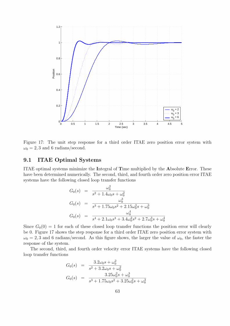
The relationship between the time domain and frequency domain is something we must be awareof when designing control systems. While we want our system to respond quickly , i.e., have asmall settling time, we have to realize what effects this has in the frequency domain. We will bedealing predominantly with lowpass systems in this course. For these systems we will define thebandwidth of a system to be that frequency ωb where the magnitude has fallen 3 dB from themagnitude at dc, or zero frequency. Hence the bandwidth defines the the half power frequencyof the system, or that frequency when
1
2|H(0)|2 = |H(jωb)|2
Consider a first order system described by the transfer function
G(s) =K
τs + 1=
(Kτ
)
s + 1τ
where K is the static gain and τ is the time constant. The pole of the system is a − 1τ. Assuming
the system is initially at rest, the unit step response of the system will be given by
y(t) = K(1− e−tτ )u(t)
If we want faster response, we want the time constant τ to become smaller, which means themagnitude of poles of the system become larger (the poles move farther away from the jω axis.Figure 12 displays the step response and corresponding frequency response (more precisely, themagnitude portion of the frequency response) for K/τ = 1 (this ratio is fixed) and τ = 1,τ = 1/10 and τ = 1/100, which corresponds to poles at -1, -10, and -100. As this figureindicates, as the response of the system becomes faster (in the time domain), the bandwidth ofthe system increases. For this system the bandwidth will be determined by the pole location,or ωb = 1/τ . Thus the speed of response is directly related to the bandwidth of the system.
Now let’s consider a transfer function with two distinct poles, say at −p1 and −p2, so thetransfer function is
G(s) =K
(s + p1)(s + p2)
and the unit step response for p1 6= p2 is given by
y(t) =
[K
p1p2
+K
(p1 − p2)p1
e−p1t +K
(p2 − p1)p2
e−p2t
]u(t)
Figure 13 displays the step response and corresponding frequency response when K/p1p2 = 1and p1 = 1, p2 = 2, p1 = 1, p2 = 10, and p1 = 1, p2 = 100 and Figure 14 for K/p1p2 = 1 andp1 = 6, p2 = 7, p1 = 6, p2 = 20, and p1 = 6, p2 = 40.
As these figures demonstrate, the speed of response is determined by the pole closest to thejω axis, the dominant pole. The bandwidth of the system is also determined by the dominantpole. While the second pole affects the shape of both the time and frequency response, it isthe dominant pole that really determines the speed of response and the bandwidth. Here the
52
0 1 2 3 40
0.2
0.4
0.6
0.8
1 τ = 1, p = 1/τ = 1
Dis
plac
emen
t
0 1 2 3 40
0.2
0.4
0.6
0.8
1 τ = 0.333, p = 1/τ = 3
Dis
plac
emen
t
0 1 2 3 40
0.2
0.4
0.6
0.8
1τ = 0.1, p = 1/τ = 10
Dis
plac
emen
t
Time (sec)
10−1
100
101
102
−40
−35
−30
−25
−20
−15
−10
−5
0
5
dB
ωb = 1
10−1
100
101
102
−40
−35
−30
−25
−20
−15
−10
−5
0
5
dB
ωb = 3
10−1
100
101
102
−40
−35
−30
−25
−20
−15
−10
−5
0
5
dB
ωb = 10
Frequency (rad/sec)
Figure 12: The unit step response and bandwidth for three first order systems. The magnitudeof the system pole p is equal to the bandwidth ωb.
53
0 2 4 60
0.2
0.4
0.6
0.8
1
p1 = 1, p
2 = 2
Dis
plac
emen
t
0 2 4 60
0.2
0.4
0.6
0.8
1
p1 = 1, p
2 = 10
Dis
plac
emen
t
0 2 4 60
0.2
0.4
0.6
0.8
1
p1 = 1, p
2 = 100
Dis
plac
emen
t
Time (sec)
10−1
100
101
−40
−35
−30
−25
−20
−15
−10
−5
0
5
dB
ωb = 1
10−1
100
101
−40
−35
−30
−25
−20
−15
−10
−5
0
5
dB
ωb = 1
10−1
100
101
−40
−35
−30
−25
−20
−15
−10
−5
0
5
dB
ωb = 1
Frequency (rad/sec)
Figure 13: The unit step response and bandwidth for three second order systems with distinctpoles. The rate of response is dominated by the dominant pole at -1, and the bandwidth (-3 dBpoint) is determined by this dominant pole.
54
0 0.5 1 1.50
0.2
0.4
0.6
0.8
1
p1 = 6, p
2 = 7
Dis
plac
emen
t
0 0.5 1 1.50
0.2
0.4
0.6
0.8
1
p1 = 6, p
2 = 20
Dis
plac
emen
t
0 0.5 1 1.50
0.2
0.4
0.6
0.8
1
p1 = 6, p
2 = 40
Dis
plac
emen
t
Time (sec)
100
101
102
−40
−35
−30
−25
−20
−15
−10
−5
0
5
dB
ωb = 6
100
101
102
−40
−35
−30
−25
−20
−15
−10
−5
0
5
dB
ωb = 6
100
101
102
−40
−35
−30
−25
−20
−15
−10
−5
0
5
dB
ωb = 6
Frequency (rad/sec)
Figure 14: The unit step response and bandwidth for three second order systems with distinctpoles. The rate of response is dominated by the dominant pole at -6, and the bandwidth (-3 dBpoint) is determined by this dominant pole.
55
bandwidth is determined by ωb = min(p1, p2). Clearly, if we were to add additional distinctpoles to this system, the response would be determined by the dominant poles.
Now let’s look at a system with complex conjugate poles, such as our ideal second ordersystem. For an ideal second order system with transfer function
G(s) =K
1ωn
2s2 + 2ζ
ωns + 1
=Kω2
n
s2 + 2ζωns + ω2n
the poles are located at −ζωn±jωd, which is commonly written as −σ± jωd. The characteristicmodes that go with these poles are of the form
e−σt cos(ωdt)
e−σt sin(ωdt)
Hence the speed of response will be governed by σ, which is the real part of the pole. Thebandwidth of the system is more complicated to determine. As a simple rule, for a fixed ωd
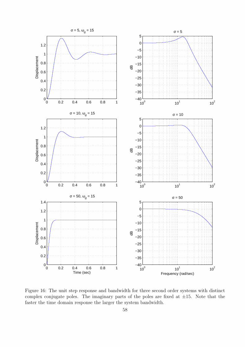
(the imaginary part of the pole), as σ gets larger the bandwidth gets larger. Figures 15 and 16display the both the step and frequency responses (magnitude only) of an ideal second ordersystems with complex poles at [ −5 ± 4j, −10 ± 4j, −50 ± 4j] and [−5 ± 15j, −10 ± 15j,−50± 15j], respectively. Note again, comparing these figures, that it is the real part of the polethat determines the settling time, not the imaginary part.
Why, you might ask, do we care about the bandwidth? There are two reasons. The first isthat the bandwidth tells us the types of signals our system will be able to follow. We all knowthat if the input to a system G(s) is x(t) = Acos(ω0t), that in steady state the output of thesystem will be given by
y(t) = A|G(jω0)| cos(ω0t + 6 G(jω0))
Hence if the input to our system oscillates “faster” than cos(ωbt), or has higher frequency contentthan ωb, where ωb is the bandwidth, our system will not be able to follow this input very well.More accurately, the output of the system will oscillate at the same frequency as the input, butwith a substantially reduced amplitude.
The second reason we care about bandwidth is that all real systems have noise in them.This noise is often introduced to the system by the sensors we need to make measurements,such as measuring the system position or velocity. A fairly reasonable model for noise iswhite noise. White noise is basically modelled as having constant power spectral density (thepower/frequency) of N0/2, or
Sxx(ω) =N0
2
If the noise is the input to a system with transfer function G(ω), then the output power spectraldensity Syy(ω)is given by
Syy(ω) = |G(ω)|2Sxx(ω)
= |G(ω)|2N0
2
56
0 0.2 0.4 0.6 0.8 10
0.2
0.4
0.6
0.8
1
1.2
σ = 5, ωd = 4
Dis
plac
emen
t
0 0.2 0.4 0.6 0.8 10
0.2
0.4
0.6
0.8
1
1.2
σ = 10, ωd = 4
Dis
plac
emen
t
0 0.2 0.4 0.6 0.8 10
0.2
0.4
0.6
0.8
1
1.2
1.4
σ = 50, ωd = 4
Dis
plac
emen
t
Time (sec)
100
101
102
−40
−35
−30
−25
−20
−15
−10
−5
0
5
dB
σ = 5
100
101
102
−40
−35
−30
−25
−20
−15
−10
−5
0
5
dB
σ = 10
100
101
102
−40
−35
−30
−25
−20
−15
−10
−5
0
5
dB
σ = 50
Frequency (rad/sec)
Figure 15: The unit step response and bandwidth for three second order systems with distinctcomplex conjugate poles. The imaginary parts of the poles are fixed at ±4. Note that the fasterthe time domain response the larger the system bandwidth.
57
0 0.2 0.4 0.6 0.8 10
0.2
0.4
0.6
0.8
1
1.2
σ = 5, ωd = 15
Dis
plac
emen
t
0 0.2 0.4 0.6 0.8 10
0.2
0.4
0.6
0.8
1
1.2
σ = 10, ωd = 15
Dis
plac
emen
t
0 0.2 0.4 0.6 0.8 10
0.2
0.4
0.6
0.8
1
1.2
1.4
σ = 50, ωd = 15
Dis
plac
emen
t
Time (sec)
100
101
102
−40
−35
−30
−25
−20
−15
−10
−5
0
5
dB
σ = 5
100
101
102
−40
−35
−30
−25
−20
−15
−10
−5
0
5
dB
σ = 10
100
101
102
−40
−35
−30
−25
−20
−15
−10
−5
0
5
dB
σ = 50
Frequency (rad/sec)
Figure 16: The unit step response and bandwidth for three second order systems with distinctcomplex conjugate poles. The imaginary parts of the poles are fixed at ±15. Note that thefaster the time domain response the larger the system bandwidth.
58
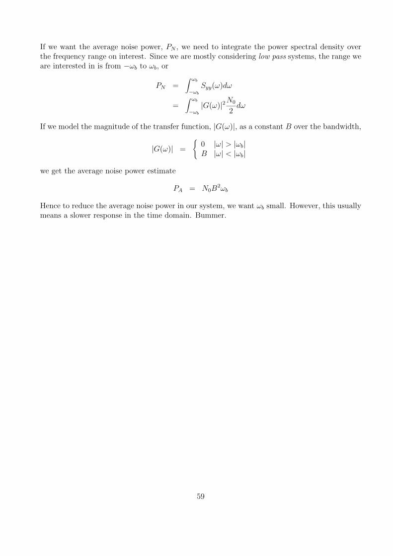
If we want the average noise power, PN , we need to integrate the power spectral density overthe frequency range on interest. Since we are mostly considering low pass systems, the range weare interested in is from −ωb to ωb, or
PN =∫ ωb
−ωb
Syy(ω)dω
=∫ ωb
−ωb
|G(ω)|2N0
2dω
If we model the magnitude of the transfer function, |G(ω)|, as a constant B over the bandwidth,
|G(ω)| =
{0 |ω| > |ωb|B |ω| < |ωb|
we get the average noise power estimate
PA = N0B2ωb
Hence to reduce the average noise power in our system, we want ωb small. However, this usuallymeans a slower response in the time domain. Bummer.
59
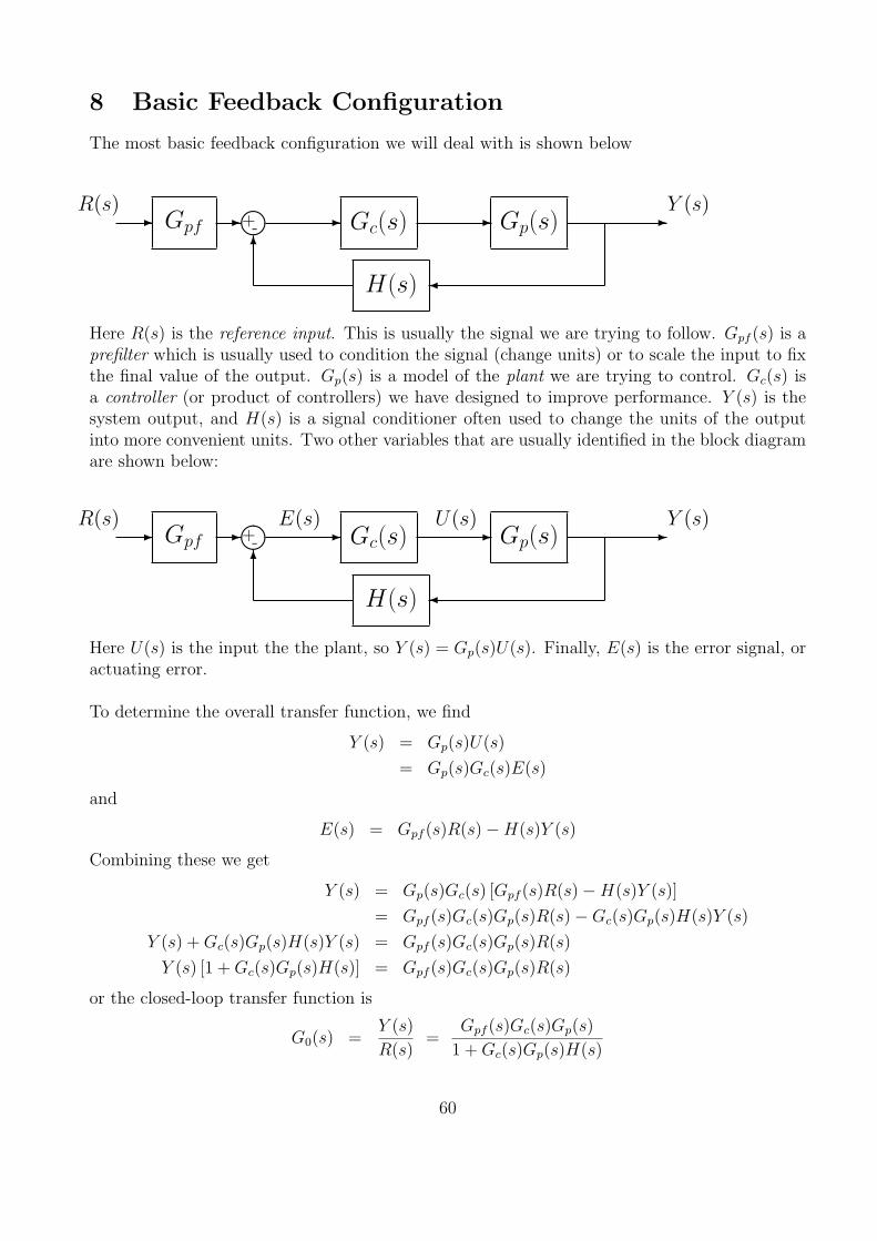
8 Basic Feedback Configuration
The most basic feedback configuration we will deal with is shown below
R(s)- Gpf
-±°²¯
- Gc(s) - Gp(s) -Y (s)
¾H(s)
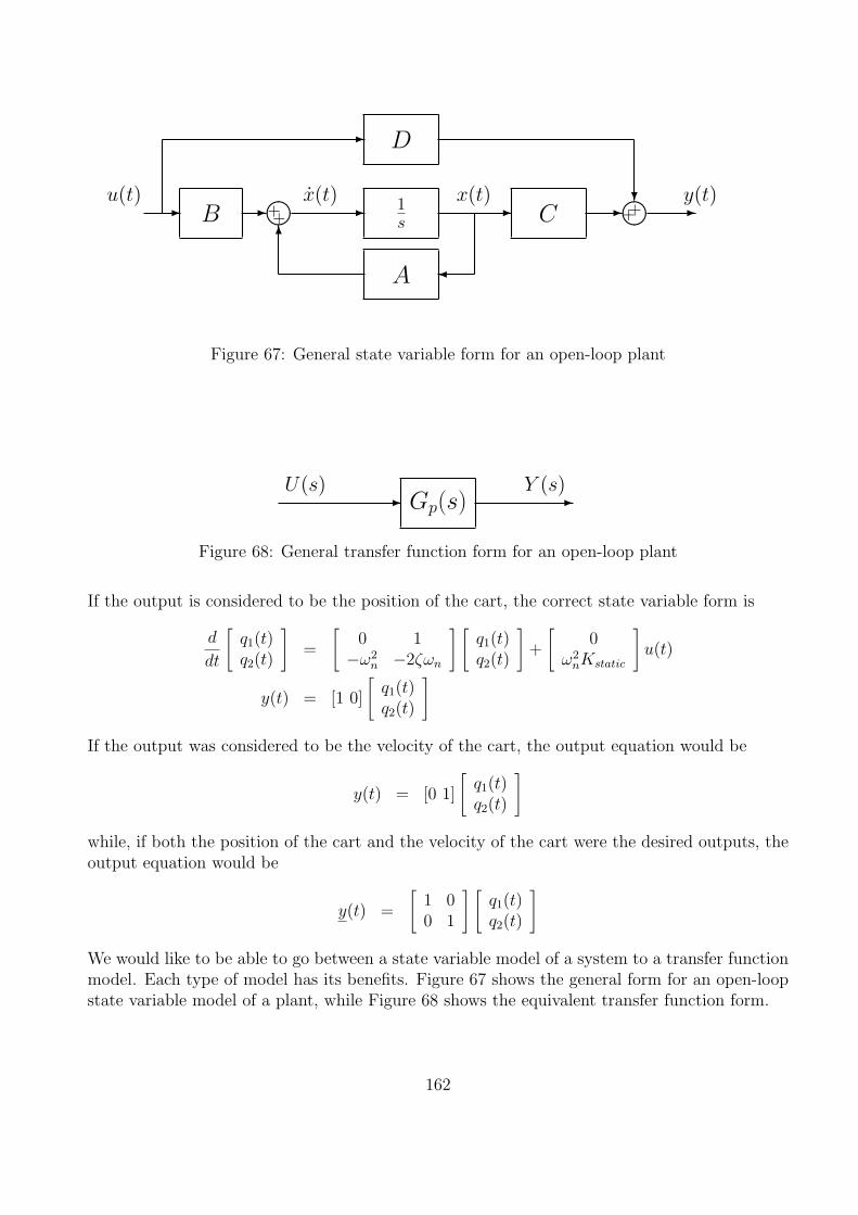
6
+-
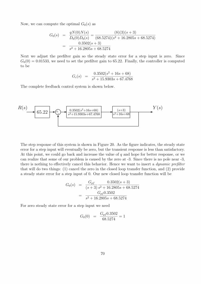
Here R(s) is the reference input. This is usually the signal we are trying to follow. Gpf (s) is aprefilter which is usually used to condition the signal (change units) or to scale the input to fixthe final value of the output. Gp(s) is a model of the plant we are trying to control. Gc(s) isa controller (or product of controllers) we have designed to improve performance. Y (s) is thesystem output, and H(s) is a signal conditioner often used to change the units of the outputinto more convenient units. Two other variables that are usually identified in the block diagramare shown below:
R(s)- Gpf
-±°²¯
-E(s)
Gc(s) -U(s)
Gp(s) -Y (s)
¾H(s)
6
+-
Here U(s) is the input the the plant, so Y (s) = Gp(s)U(s). Finally, E(s) is the error signal, oractuating error.
To determine the overall transfer function, we find
Y (s) = Gp(s)U(s)
= Gp(s)Gc(s)E(s)
and
E(s) = Gpf (s)R(s)−H(s)Y (s)
Combining these we get
Y (s) = Gp(s)Gc(s) [Gpf (s)R(s)−H(s)Y (s)]
= Gpf (s)Gc(s)Gp(s)R(s)−Gc(s)Gp(s)H(s)Y (s)
Y (s) + Gc(s)Gp(s)H(s)Y (s) = Gpf (s)Gc(s)Gp(s)R(s)
Y (s) [1 + Gc(s)Gp(s)H(s)] = Gpf (s)Gc(s)Gp(s)R(s)
or the closed-loop transfer function is
G0(s) =Y (s)
R(s)=
Gpf (s)Gc(s)Gp(s)
1 + Gc(s)Gp(s)H(s)
60
9 Model Matching
The first type of control scheme we will discuss is that of model matching. Here, we assume wehave a plant Gp(s) with a controller Gc(s) in a untiy feedback scheme, as shown below.
-½¼
¾»- Gc(s) - Gp(s) -
6
+-
For this closed-loop feedback system, the closed-loop transfer function G0(s) is given by
G0(s) =Gc(s)Gp(s)
1 + Gc(s)Gp(s)
The object of this course is to determine how to choose the controller Gc(s) so the overall systemmeets some design criteria. The idea behind model matching is to assume we know what wewant the closed loop transfer function G0(s) to be. Then, since G0(s) and Gp(s) are known, wecan determine the controller Gc(s) as
[1 + Gc(s)Gp(s)] G0(s) = Gc(s)Gp(s)
G0(s) + Gc(s)Gp(s)G0(s) = Gc(s)Gp(s)
G0(s) = Gc(s)Gp(s)−Gc(s)Gp(s)G0(s)
G0(s) = Gc(s)Gp(s) [1−G0(s)]
or
Gc(s) =G0(s)
Gp(s) [1−G0(s)]
If we write Gp(s) = N(s)D(s)
and G0(s) = N0(s)D0(s)
, we can rewrite this as
Gc(s) =N0(s)D(s)
D0(s)N(s)−N(s)N0(s)
This form is often easier to work with. However, we still have to be careful to eliminate commonfactors from the numerator and denominator.
61
While this type of model matching looks simple, there are certain restrictions on when thiswill work. The closed loop transfer function G0(s) is said to be implementable if1
1. The controller Gc(s) is a proper rational transfer function
2. The controller Gc(s) is stable
Consider a plant with proper transfer function Gp(s) = N(s)D(s)
where we want the closed loop
transfer function to be G0(s) = N0(s)D0(s)
. We can find a Gc(s) so that G0(s) is implementable onlyunder the following conditions:
1. The degree of D0(s) - the degree of N0(s) ≥ the degree D(s) - the degree of N(s)
2. All right half plane zeros of N(s) are retained in N0(s) (the RHP zeros of the plant mustalso be in the closed-loop transfer function)
3. G0(s) is stable, i.e., all poles of G0(s) are in the left half plane (none on the axes)
Example 1. Consider the system with plant
Gp(s) =(s + 2)(s− 1)
s(s2 − 2s + 2)
Are the following closed loop transfer functions implementable?
1. G0(s) = 1. (No, it violates (1) and (2))
2. G0(s) = (s+2)(s+3)(s+1)
. (No, violates (2))
3. G0(s) = (s−1)(s+3)(s+1)
. (Yes)
4. G0(s) = (s−1)s(s+2)
. (No, violates (3))
5. G0(s) = (s−1)(s+3)(s+1)2
. (Yes)
6. G0(s) = (s−1)(2s−3)(s+2)3
. (Yes)
Now that we know when we can use model matching, we need to find some good models. That is,how do we find a desirable G0(s)? We will look at four possible choices, ITAE optimal systems,deadbeat systems, quadratic optimal systems, and steady state frequency response matching.
1There are other restrictions, but they are not important in this course.
62
0 0.5 1 1.5 2 2.5 3 3.5 4 4.5 50
0.2
0.4
0.6
0.8
1
1.2
Time (sec)
Pos
ition
ω0 = 2
ω0 = 3
ω0 = 6
Figure 17: The unit step response for a third order ITAE zero position error system withω0 = 2, 3 and 6 radians/second.
9.1 ITAE Optimal Systems
ITAE optimal systems minimize the Integral of Time multiplied by the Absolute Error. Thesehave been determined numerically. The second, third, and fourth order zero position error ITAEsystems have the following closed loop transfer functions
G0(s) =ω2
0
s2 + 1.4ω0s + ω20
G0(s) =ω3
0
s3 + 1.75ω0s2 + 2.15ω20s + ω3
0
G0(s) =ω4
0
s4 + 2.1ω0s3 + 3.4ω20s
2 + 2.7ω30s + ω4
0
Since G0(0) = 1 for each of these closed loop transfer functions the position error will clearlybe 0. Figure 17 shows the step response for a third order ITAE zero position error system withω0 = 2, 3 and 6 radians/second. As this figure shows, the larger the value of ω0, the faster theresponse of the system.
The second, third, and fourth order velocity error ITAE systems have the following closedloop transfer functions
G0(s) =3.2ω0s + ω2
0
s2 + 3.2ω0s + ω20
G0(s) =3.25ω2
0s + ω30
s3 + 1.75ω0s2 + 3.25ω20s + ω3
0
63
0 0.5 1 1.5 2 2.5 3 3.5 4 4.5 50
0.2
0.4
0.6
0.8
1
1.2
1.4
Time (sec)
Pos
ition
ω0 = 2
ω0 = 3
ω0 = 6
Figure 18: The unit step response for a third order ITAE zero velocity error system with ω0 = 2, 3and 6 radians/second.
G0(s) =5.14ω3
0s + ω40
s4 + 2.41ω0s3 + 4.93ω20s
2 + 5.14ω30s + ω4
0
Since the coefficients of s1 and s0 are identical for both the numerator and denominator of theseclosed loop transfer functions, both the position and velocity errors will be zero. Figure 18shows the step response for a third order ITAE zero velocity error system with ω0 = 2, 3 and 6radians/second. As this figure shows, we are paying for zero velocity error with a substantialovershoot. As with the ITAE zero position error systems, the larger the value of ω0, the fasterthe response of the system.
You, the designer, need to choose the value of ω0. The larger the ω0, the faster the systemresponds (good) and the larger the control effort (bad).
9.2 Deadbeat Systems
A deadbeat response is a response that that proceeds rapidly to the desired level and holds thatlevel with minimal overshoot. These have also been determined numerically. The second, third,and fourth order closed loop transfer functions for deadbeat control are
G0(s) =ω2
0
s2 + 1.82ω0s + ω20
G0(s) =ω3
0
s3 + 1.90ω0s2 + 2.20ω20s + ω3
0
64
0 0.5 1 1.5 2 2.5 3 3.5 4 4.5 50
0.2
0.4
0.6
0.8
1
1.2
Time (sec)
Pos
ition
ω0 = 2
ω0 = 3
ω0 = 6
Figure 19: The unit step response for a third order deadbeat system with ω0 = 2, 3 and 6radians/second.
G0(s) =ω4
0
s4 + 2.20ω0s3 + 3.50ω20s
2 + 2.80ω30s + ω4
0
Since G0(0) = 1 for each of these closed loop transfer functions, it should be clear that we willhave ep = 0. However the velocity error will not be zero. Figure 19 shows the step response fora third order deadbeat response for ω0 = 2, 3 and 6 radians/second. Comparing Figure 19 withFigure 17, it is clear that the ITAE and deadbeat responses are quite similar. This is also clearby examining the transfer functions. As with the ITAE systems, the larger the value of ω0 thefaster the response of the system (good) and the more control effort (bad) required.
9.3 Quadratic Optimal Systems
For a quadratic optimal system, we want to find the closed loop transfer function G0(s) tominimize the quadratic performance index
J =∫ ∞
0
{q [y(t)− r(t)]2 + u2(t)
}dt
where y(t) is the output of the system, r(t) is the input to the system, q is a positive constantthat weighs the difference between the input to the system and the output to the system, andu(t) is the actuating signal (the input to the plant we are trying to control). In general, forthis type of controller, we want the output of our system to match (or track) the input to the
65
system. To determine G0(s) to solve this problem, we need to first discuss spectral factorization.
Consider first the plant with proper transfer function Gp(s) = N(s)D(s)
where D(s) and N(s) haveno common factors. Next, consider the polynomial
Q(s) = D(s)D(−s) + qN(s)N(−s)
Clearly Q(−s) = Q(s), hence if s1 is a root of Q(s), then so is −s1. Since all of the coefficientsof Q(s) are real by assumption (we assume Gp(s) is real), if s1 is a root of Q(s) than so is itscomplex conjugate s∗1. Hence, all of the roots of Q(s) are symmetric with respect to
• the real axis
• the imaginary axis
• the origin of the s-plane
Now consider
Q(jω) = D(jω)D(−jω) + qN(jω)N(−jω)
= |D(jω)|2 + q|N(jω)|2
Since D(s) and N(s) have no common factors, there exists no ω0 so that both D(jω0) = 0 andN(jω0) = 0. Since q 6= 0, there exists no ω0 so that Q(ω0) = 0. Hence Q(s) has no roots onthe jω axis.
Since the roots of Q(s) are either in the left half plane or the right half plane (none on thejω axis), and since, by symmetry, there will be an equal number in each plane, we will divideup the roots of Q(s) into those in the open LHP and those in the open RHP. Let’s denote thepolynomial whose roots are those of the open LHP roots of Q(s) as D0(s). Then, by symmetry,D0(−s) is a polynomial whose roots are the open RHP roots of Q(s). Thus,
Q(s) = D(s)D(−s) + qN(s)N(−s) = D0(s)D0(−s)
This is called the spectral factorization of Q(s). Now we can give the result.
Consider a plant with proper transfer function Gp(s) = N(s)/D(s) where
• N(s) and D(s) have no common factors
• The leading coefficient of D(s) (the coefficient of the highest power of s in D(s)) is 1.That is, D(s) is monic. This is important!
An implementable transfer function G0(s) that minimizes the performance index
J =∫ ∞
0
{q [y(t)− r(t)]2 + u2(t)
}dt
where r(t) = 1 (a unit step) and q > 0 is given by
G0(s) =qN(0)N(s)
D0(0)D0(s)
66
where
Q(s) = D(s)D(−s) + qN(s)N(−s) = D0(s)D0(−s)
Note that we are not guaranteed a zero position error with this method. For a zero positionerror, we should have G0(0) = 1. In addition, if N(s) = s this will not work (since N(0) = 0).
Example 2. Suppose we have the plant with transfer function
Gp(s) =1
s2 + 1
and we want to find G0(s) to minimize
J =∫ ∞
0
{10 [y(t)− r(t)]2 + u2(t)
}dt
Clearly q = 10, Gp(s) is a proper transfer function, N(s) and D(s) have no common factors,and D(s) is a monic polynomial. Now N(s) = 1, D(s) = s2 + 1, and D(s) is monic. So we have
D(s) = s2 + 1 N(s) = 1
D(−s) = s2 + 1 N(−s) = 1
and
Q(s) = D(s)D(−s) + qN(s)N(−s)
=[s2 + 1
] [s2 + 1
]+ 10 [1] [1]
=[s4 + 2s2 + 1
]+ 10 [1]
= s4 + 2s2 + 11
Note that Q(s) is an even function of s. If it is not, you screwed up! Now, we need to find theroots of Q(s). These roots are −1.0762± 1.4691j and 1.0762± 1.4969j. To construct D0(s), weuse only those roots in the LHP, i.e. the roots at −1.0762± 1.4691.
D0(s) = (s + 1.0762− 1.4691j)(s + 1.0762 + 1.4691j)
D0(s) = s2 + 2.1525s + 3.3166
Now, we can compute the optimal G0(s) as
G0(s) =qN(0)N(s)
D0(0)D0(s)=
(10)(1)(1))
(3.3166)(s2 + 2.1525s + 3.3166)
=3.01514
s2 + 2.1525s + 3.3166
Note that G0(0) = 0.909, which yields a position error of ep = 0.091. To achieve a position errorof zero we need a prefilter with a value of Gpf = 1/0.909 = 1.100. Finally, to determine thecontroller, we use the formula
Gc(s) =G0(s)
Gp(s) (1−G0(s))
67
which produces the controller
Gc(s) =1.401s2 + 1.401
0.4646s2 + s + 0.1401
=1.401[s2 + 1]
0.4646s2 + s + 0.1401
Note that the controller has been scaled, and there will be a pole/zero cancellation between theplant and the controller. Since these are marginally stable poles, this may not be a good idea.
Example 3. Suppose we have the plant with transfer function
Gp(s) =0.3(s + 2)
0.01s2 + 0.2s + 1
and we want to find G0(s) to minimize
J =∫ ∞
0
{15 [y(t)− r(t)]2 + u2(t)
}dt
Clearly q = 15, Gp(s) is a proper transfer function, and N(s) and D(s) have no common factors.However, before we use the algorithm, we must be sure D(s) is a monic polynomial. To do this,we multiply both the top and bottom by 100
Gp(s) =100
100
0.3(s + 2)
0.01s2 + 0.2s + 1=
30(s + 2)
s2 + 20s + 100
Now N(s) = 30(s + 2), D(s) = s2 + 20s + 100, and D(s) is monic. So we have
D(s) = s2 + 20s + 100 N(s) = 30(s + 2)
D(−s) = s2 − 20s + 100 N(−s) = 30(−s + 2)
and
Q(s) = D(s)D(−s) + qN(s)N(−s)
=[s2 + 20s + 100
] [s2 − 20s + 100
]+ 15 [30(s + 2)] [30(−s + 2)]
=[s4 − 200s2 + 10000
]+ 15
[−900s2 + 3600
]
= s4 − 13, 700s2 + 64, 000
Note that Q(s) is an even function of s. If it is not, you screwed up! Now we need to find theroots of Q(s). These roots are ±117.027 and ±− 2.161. To construct D0(s) we use only thoseroots in the LHP, i.e., the roots at -117.027 and -2.161
D0(s) = (s + 117.027)(s + 2.161)
D0(s) = s2 + 119.2s + 252.9
Now, we can compute the optimal G0(s) as
G0(s) =qN(0)N(s)
D0(0)D0(s)=
(15)(60)30(s + 2)
(252.9)(s2 + 119.2s + 252.9)
=106.7(s + 2)
s2 + 119.2s + 252.9
68
Note that G0(0) = 0.8438, which yields a steady state error for a step input of ess = 0.156. Fora steady state error of zero we would need a prefilter with a value of Gpf = 1/0.8438 = 1.185.Finally, to determine the controller, we use the formula
Gc(s) =G0(s)
Gp(s) (1−G0(s))
which produces the controller
Gc(s) =0.09s2 + 1.8s + 9
0.0253s2 + 0.3153s + 1
=0.09[s2 + 20s + 100]
0.0253s2 + 0.3153s + 1
Note that this controller has been scaled and there is a pole/zero cancellation between the con-troller and the plant. The poles being cancelled are stable poles, so this is probably acceptable.
9.4 Dynamic Prefilters
Up to this point, we have used only constant prefilters Gpf to scale the input to achieve thedesired position error. However, sometimes the plant or the controller introduces zeros into theclosed loop transfer function that we do not want. One way to eliminate these zeros is with adynamic prefilter, Gpf (s). This is best illustrated with an example.
Example 4. Suppose we have the plant with transfer function
Gp(s) =(s + 3)
s2 + 16s + 68
and we want to find G0(s) to minimize
J =∫ ∞
0
{8 [y(t)− r(t)]2 + u2(t)
}dt
Clearly q = 8, Gp(s) is a proper transfer function, N(s) and D(s) have no common factors, andD(s) is a monic polynomial. Now N(s) = (s + 3), D(s) = s2 + 16s + 68. So we have
D(s) = s2 + 16s + 68 N(s) = (s + 3)
D(−s) = s2 − 16s + 68 N(−s) = (−s + 3)
and
Q(s) = D(s)D(−s) + qN(s)N(−s)
=[s2 + 16s + 68
] [s2 − 16s + 68
]+ 8 [(s + 3)] [(−s + 3)]
= s4 − 128s2 + 4696
Note that Q(s) is an even function of s. If it is not, you screwed up! Now we need to find theroots of Q(s). These roots are ±8.1403± j1.5046. To construct D0(s) we use only those rootsin the LHP, i.e., the roots at −8.1403 + j1.5046 and −8.1403− j1.5046
D0(s) = (s + 8.1403− j1.5046)(s + 8.1403 + j1.5046)
D0(s) = s2 + 16.2805s + 68.5274
69
Now, we can compute the optimal G0(s) as
G0(s) =qN(0)N(s)
D0(0)D0(s)=
(8)(3)(s + 3)
(68.5274)(s2 + 16.2805s + 68.5274)
=0.3502(s + 3)
s2 + 16.2805s + 68.5274
Next we adjust the prefilter gain so the steady state error for a step input is zero. SinceG0(0) = 0.01533, we need to set the prefilter gain to 65.22. Finally, the controller is computedto be
Gc(s) =0.3502(s2 + 16s + 68)
s2 + 15.9303s + 67.4768
The complete feedback control system is shown below.
R(s)- 65.22 -±°
²- 0.3502(s2+16s+68)
s2+15.9303s+67.4768- (s+3)
s2+16s+68-
Y (s)
6
+-
The step response of this system is shown in Figure 20. As the figure indicates, the steady stateerror for a step input will eventually be zero, but the transient response is less than satisfactory.At this point, we could go back and increase the value of q and hope for better response, or wecan realize that some of our problem is caused by the zero at -3. Since there is no pole near -3,there is nothing to effectively cancel this behavior. Hence we want to insert a dynamic prefilterthat will do two things: (1) cancel the zero in the closed loop transfer function, and (2) providea steady state error for a step input of 0. Our new closed loop transfer function will be
G0(s) =Gpf
(s + 3)
0.3502(s + 3)
s2 + 16.2805s + 68.5274
=Gpf0.3502
s2 + 16.2805s + 68.5274
For zero steady state error for a step input we need
G0(0) =Gpf0.3502
68.5274= 1
70
0 0.5 1 1.50
0.2
0.4
0.6
0.8
1
1.2
1.4
Time (sec)
Pos
ition
Figure 20: The unit step response of quadratic optimal system from Example 4, utilizing onlya constant prefilter Gpf = 65.22.
or Gpf = 195.68. The complete control system with the dynamic prefilter is shown below:
R(s)- 195.68
(s+3)-±°
²- 0.3502(s2+16s+68)
s2+15.9303s+67.4768- (s+3)
s2+16s+68-
Y (s)
6
+-
Figure 21 show the step response with the dynamic prefilter. Note the percent overshoot hasbeen essentially eliminated, and the transient behavior is now more like that of an overdampedor critically damped ideal second order system.
While the dynamic prefilter has eliminated the zero from the closed loop transfer function,and improved the transient response, it should be noted that the prefilter is outside the feedbackloop. In many instances this is not a problem, however, any value outside the feedback loopis more sensitive to parameter variation and drift than values or transfer functions inside thefeedback loop. We’ll have more to say about this when we discuss system sensitivity later.
71
0 0.5 1 1.50
0.1
0.2
0.3
0.4
0.5
0.6
0.7
0.8
0.9
1
Time (sec)
Pos
ition
Figure 21: The unit step response of quadratic optimal system from Example 4, utilizing adynamic prefilter Gpf = 195.6808
(s+3).
9.5 Type One Systems
The method we have presented for determining the quadratic optimal controller will always giveus a stable controller. However, sometimes we might want to change this method slightly whichmay either give us an even better controller, or perhaps one which is unstable and thereforeunusable. In our next chapter we will start discussing different system types and how they helpus determine system parameters such as position and velocity errors very quickly. However, atthis point we will revisit two of our previous examples and remove the need for the prefilter.This will mean that we have no blocks outside the feedback loop and, for these examples, pro-duce what are called type 1 systems. The general idea is to take the transfer function G0(s)determined by the quadratic optimal formula, and scale it directly so G0(0) = 1, thus avoidingthe need for a prefilter.
Example 2 (Again). Here we have the plant
Gp(s) =1
s2 + 1
and we determined that for q = 10 we should have the closed loop transfer function
G0(s) =3.01514
s2 + 2.1525s + 3.3166
72
and the corresponding controller
Gc(s) =1.401[s2 + 1]
0.4646s2 + s + 0.1401
and prefilter
Gpf = 1.1001
Now, instead, let’s modify G0(s) so that G0(0) = 1. The easiest way to do this is to multiplyby the prefilter value, so
G0(s) =1.100 ∗ 3.01514
s2 + 2.1525s + 3.3166
=3.3166
s2 + 2.152s + 3.3166
Clearly G0(0) = 1. Next we compute Gc(s) as before, to get
Gc(s) =3.015[s2 + 1]
s2 + 2.212s
Note that now we can factor 1s
from the controller, which we could not do before. This is a goodthing.
Example 3 (Again). Here we have the plant
Gp(s) =30(s + 2)
s2 + 20s + 100
and we determined that for q = 15 we should have the closed loop transfer function
G0(s) =106.7(s + 2)
s2 + 119.2s + 252.9
and the corresponding controller
Gc(s) =0.09[s2 + 20s + 100]
0.0253s2 + 0.3153s + 1
and prefilter
Gpf = 1.1851
Now, instead, let’s modify G0(s) so that G0(0) = 1. The easiest way to do this is to multiplyby the prefilter value, so
G0(s) =1.1851 ∗ 106.7[s + 2]
s2 + 119.2s + 252.9
=126.45[s + 2]
s2 + 119.2s + 252.9
73
Clearly G0(0) = 1. Next we compute Gc(s) as before, to get
Gc(s) =0.4215[s2 + 20s + 100]
s2 − 7.25s
Note that now we can factor 1s
from the controller, which we could not do before. This is agood thing. However, our controller is no longer stable, which means we would not want toimplement it and would use our original controller.
9.6 Frequency Response Matching
Although all of the model matching method presented so far have been time domain models,we need to keep in mind the fact that everything we do in the time-domain has an effect inthe frequency domain. Thus, when we have designed a closed loop control system with transferfunction G0(s), we have to realize that we have really constructed a filter between the input andoutput signal! Hence, if the input to our system is u(t) = A cos(ωt + θ) the steady state outputto our system will be given by
y(t) = A|G0(jω)| cos(ωt + θ + 6 G0(jω))
Example 5. Assume we have designed a controller using model matching techniques so theclosed loop transfer function G0(s) is that of a third order deadbeat system
G0(s) =ω3
0
s3 + 1.90ω0s2 + 2.20ω20s + ω3
0
The step response for this system with ω0 = 10 rad/sec is shown in Figure 22 and the Bodeplot for this system is shown in Figure 23. For this system the bandwidth is the same as ω0,about 10 rad/sec. Now, in addition to the step response, we may also be interested in how wellour system tracks input signals of varying frequencies. Figures 24 and 25 display the output ofour control system/filter when the input consists of sine waves with unit amplitude and varyingfrequencies, from ω = 0.25ω0 to ω = 2ω0. These figures display the same information that theBode plot does in a different way. For input frequencies between 0 and ω0, the output signalhas a magnitude of 1 (for zero frequency) down to 0.707 (for ω = ω0). As the input frequencyincreases beyond ω0, the amplitude of the output decreases substantially. In addition to theamplitude, we usually need to worry about the phase. In a control system we usually want theoutput to equal the input, in both magnitude and phase. For this system we see that as theinput frequencies increase, the phase difference between the input and output signals increases,which corresponds to a longer delay between the input and output signal.
Although in the majority of this course we are concerned with following time-domain signalssuch as steps and ramps, it may be important sometimes to be able to design a system thatmeets certain frequency domain criteria. One way we can approach this is again by using amodel matching method. However, this method assumes you can determine a transfer functionthat meets the required frequency domain requirements and is still implementable.
74
0 0.1 0.2 0.3 0.4 0.5 0.6 0.7 0.8 0.9 10
0.2
0.4
0.6
0.8
1
1.2
1.4
Time (sec)
Pos
ition
Figure 22: The unit step response of the third order deadbeat system from Example 5 (ω0 = 10rad/sec.)
−120
−100
−80
−60
−40
−20
0
Mag
nitu
de (
dB)
10−1
100
101
102
103
−270
−180
−90
0
Pha
se (
deg)
Frequency (rad/sec)
Figure 23: The Bode plot of the third order deadbeat system from Example 5 (ω0 = 10 rad/sec.)
75
0 1 2 3 4 5 6−1
−0.5
0
0.5
1
ω = 0.25 ω0
InputOutput
0 1 2 3 4 5 6−1
−0.5
0
0.5
1
ω = 0.5 ω0
InputOutput
0 1 2 3 4 5 6−1
−0.5
0
0.5
1
ω = 0.75 ω0
InputOutput
0 1 2 3 4 5 6−1
−0.5
0
0.5
1
ω = ω0
Time (sec)
InputOutput
Figure 24: The response of the third order deadbeat system from Example 5 (ω0 = 10 rad/sec)to input sine waves with amplitude 1 of varying frequency ω ≤ ω0.
76
0 1 2 3 4 5 6−1
−0.5
0
0.5
1
ω = 1.25 ω0
InputOutput
0 1 2 3 4 5 6−1
−0.5
0
0.5
1
ω = 1.5 ω0
InputOutput
0 1 2 3 4 5 6−1
−0.5
0
0.5
1
ω = 1.75 ω0
InputOutput
0 1 2 3 4 5 6−1
−0.5
0
0.5
1
ω = 2ω0
Time (sec)
InputOutput
Figure 25: The response of the third order deadbeat system from Example 5 (ω0 = 10 rad/sec)to input sine waves with amplitude 1 of varying frequency ω > ω0.
77
−15
−10
−5
0
Mag
nitu
de (
dB)
100
101
102
103
−45
0
45
Pha
se (
deg)
Frequency (rad/sec)
Figure 26: The frequency response of a notch filter with ω0 = 6π and ζ0 = 0.1.
Example 6. Let’s assume that we have a plant with the transfer function
Gp(s) =10
s2 + s + 2
In addition, let’s assume we want to have zero steady state error for a step input and the outputtrack the input as well as possible. However, any input signal at 3 Hz is to be eliminated since itis likely to be interference from another part of the system. Hence we want our control systemto look something like a notch filter. One example of a second order notch filter is given by atransfer function of the form
Gn(s) =s2 + 2ζ0ω0s + ω2
0
s2 + ω0s + ω20
Here ω0 is the notch frequency and ζ0 controls the width of the notch. Since we want toeliminate input signals with frequencies at 3∗2π radians/sec, we set ωc = 6π = 18.8 radians/sec.Figures 26, 27 and 28 display the Bode plot of this filter for ζ0 = 0.1, 0.01, and 0.001, respectively.Figures 29 and 30 show the time domain response for input sin waves of various frequencies forthe notch filter shown in 28, i.e., with ω0 = 6π and ζ0 = 0.001. As these figures demonstrate, asthe frequency of the input sine wave increases towards ω0, there is a lag between the input andoutput signals, while as the frequency of the input sine wave increases beyond ω0 the outputsignal leads the input signal until the input signal is greater than approximately 2ω0. Thesesfigures also show the steady state output of the system is zero when the input sine wave has afrequency equal to ω0. Note that this output is not always zero at this frequency, just duringsteady state.
78
−40
−35
−30
−25
−20
−15
−10
−5
0
Mag
nitu
de (
dB)
100
101
102
103
−90
−45
0
45
90
Pha
se (
deg)
Frequency (rad/sec)
Figure 27: The frequency response of a notch filter with ω0 = 6π and ζ0 = 0.01.
−60
−50
−40
−30
−20
−10
0
Mag
nitu
de (
dB)
100
101
102
103
−90
−45
0
45
90
Pha
se (
deg)
Frequency (rad/sec)
Figure 28: The frequency response of a notch filter with ω0 = 6π and ζ0 = 0.001.
79
0 0.1 0.2 0.3 0.4 0.5 0.6 0.7 0.8 0.9 1−1
−0.5
0
0.5
1
ω = 0.25 ω0
InputOutput
0 0.1 0.2 0.3 0.4 0.5 0.6 0.7 0.8 0.9 1−1
−0.5
0
0.5
1
ω = 0.5 ω0
InputOutput
0 0.1 0.2 0.3 0.4 0.5 0.6 0.7 0.8 0.9 1−1
−0.5
0
0.5
1
ω = 0.75 ω0
InputOutput
0 0.1 0.2 0.3 0.4 0.5 0.6 0.7 0.8 0.9 1−1
−0.5
0
0.5
1
ω = ω0
Time (sec)
InputOutput
Figure 29: The response of the notch filter from Example 6 ( Figure 28, ω0 = 6π rad/sec,ζ0 = 0.001) to input sine waves with amplitude 1 of varying frequency ω ≤ ω0.
80
0 0.1 0.2 0.3 0.4 0.5 0.6 0.7 0.8 0.9 1−1
−0.5
0
0.5
1
ω = 1.25 ω0
InputOutput
0 0.1 0.2 0.3 0.4 0.5 0.6 0.7 0.8 0.9 1−1
−0.5
0
0.5
1
ω = 1.5 ω0
InputOutput
0 0.1 0.2 0.3 0.4 0.5 0.6 0.7 0.8 0.9 1−1
−0.5
0
0.5
1
ω = 1.75 ω0
InputOutput
0 0.1 0.2 0.3 0.4 0.5 0.6 0.7 0.8 0.9 1−1
−0.5
0
0.5
1
ω = 2ω0
Time (sec)
InputOutput
Figure 30: The response of the notch filter from Example 6 ( Figure 28, ω0 = 6π rad/sec,ζ0 = 0.001) to input sine waves with amplitude 1 of varying frequency ω > ω0.
81
This transfer function seems to accomplish what we want reasonably well, so we might betempted to try and determine the controller directly using the formula
Gc(s) =G0(s)
Gp(s)(1−G0(s))
as before. However, there is a problem. In order for G0(s) to be implementable we need tomatch the three conditions in the beginning of this chapter. The only one we will have difficultywith is (1): the degree of D0(s) - degree of N0(s) ≥ degree D(s) - degree N(s). For this notchsystem we have degree D0(s) - degree N0(s) = 0 and degree D(s) - degree N(s) = 2. It lookslike we can’t use model matching in this case. However, we can if we think a little bit and thenmodify our desired system.
In any real system all of the input signals we care about will be bandlimited, i.e., they willhave not frequency content above a certain frequency. One way to think about this is to thinkabout the Fourier series representation for a periodic signal x(t). When we try to reconstructthe original signal by summing its Fourier series, at some point there does not seem to be anyimprovement. If we stop summing the Fourier series at the N th term in the series, then thebandwidth of the signal is approximately Nωf , where ωf is the fundamental frequency. Inaddition to the input signal, we must be aware of the fact that there is always noise in anysystem. Hence, we want to limit the bandwidth of our system to limit noise in the system whilemaking the system bandwidth large enough for any likely input signal. We have not been givenany minimum bandwidth in this problem, so let’s make a reasonable assumption that our inputsignal has no frequency content above 80 Hz. This is a fairly reasonable assumption for manymechanical systems. Hence we want to limit the bandwidth beyond 80 Hz. Since we need twopoles for our Go(s) to be implementable, let’s add two poles at 80∗2π, so the closed loop transferfunction looks like
Go(s) =s2 + 2ζ0ω0s + ω2
0
(s2 + ω0s + ω20)(s + 160π)2
While these poles help with the bandwidth, we should be aware that the also contribute to thephase of the system. Finally, we probably still want ep = 0, so we need G0(0) = 1, hence ourfinal closed loop transfer function is
G0(s) =(160π)2(s2 + 0.0120π36π2)
(s2 + 6πs + 36π2)(s + 160π)2
=252, 661.8(s2 + 0.0377s + 355.3)
(s2 + 18.8s + 355.3)(s + 502.6)2
The frequency response for this system is displayed in Figure 31. As the figure indicates, thesystem bandwidth is limited to about 80 ∗ 2π = 502.6 radians/sec and the notch will eliminatethe 3Hz signals. Figure 32 shows the step response for this system. Finally, we can determinethe controller as
There are some very large numbers in this controller, and we probably need to “balance” thecoefficients before we implement this, but that’s the subject of another class.
82
−100
−90
−80
−70
−60
−50
−40
−30
−20
−10
0
Mag
nitu
de (
dB)
100
101
102
103
104
105
−180
−90
0
90
Pha
se (
deg)
Frequency (rad/sec)
Figure 31: The frequency response of the final notch filter from Example 6. Here ω0 = 6πrad/sec, ζ0 = 0.001, and we have added two poles at 160π radians/second.
0 0.1 0.2 0.3 0.4 0.5 0.6 0.70
0.2
0.4
0.6
0.8
1
1.2
1.4
Time (sec)
Pos
ition
Figure 32: The unit step response of the final notch filter from Example 6. Here ω0 = 6πrad/sec, ζ0 = 0.001, and we have added two poles at 160π radians/second.
83
9.7 Summary and Caveates
In the first part of this section, the conditions under which it is possible to to obtain an im-plementable closed loop transfer function G0(s) have been given, it may not be possible to findsuch a G0(s) using the ITAE, deadbeat, or quadratic optimal criteria. In particular, the ITAEand deadbeat methods will not work for a system with RHP zeros in the plant.
The model matching methods we have discussed often utilize pole-zero cancellations betweenthe controller Gc(s) and the plant Gp(s) to achieve the desired closed-loop transfer function.This requires that we have a fairly good model of the plant being cancelled. If we have a goodmodel of the plant and a stable pole is being cancelled, this is usually OK. However cancellingan unstable pole is not acceptable. In addition, the plant may change over time, and we aredealing with models of the plant in the first place. Hence the pole-zero cancellations may notbe very effective for some systems.
84
10 System Type and Steady State Errors
10.1 Review
Let’s assume we have a control system in a unity feedback configuration as shown below:
-½¼
¾»- Gc(s) - Gp(s) -
6
+-
where Gp(s) is the plant transfer function and Gc(s) is a controller. Note that there is noprefilter! The closed-loop transfer function is given by
G0(s) =Gc(s)Gp(s)
1 + Gc(s)Gp(s)
We already know that if we write
G0(s) =nmsm + nm−1s
m−1 + ... + n2s2 + b1s + b0
sn + dn−1sn−1 + ... + d2s2 + d1s + d0
that the steady state error for an input step of amplitude A is given by
ess = Ad0 − n0
d0
If G0(0) = 1 (the constant terms in the numerator and denominator are the same), then ess = 0.The steady state error for an input of tA is given by
ess = Ad1 − n1
d0
If the coefficients of s1 and s0 are the same, then the steady state error for a ramp input is zero.
10.2 System Type For a Unity Feedback Configuration
Unity feedback configurations are very common, and we would like to be able to analyze thistype of system very quickly without computing the closed-loop transfer function.
Let’s assume we group the all of the transfer functions together into one transfer function, whichwe will call G(s), so G(s) = Gc(s)Gp(s). Assume we write G(s) as2
G(s) =K(Tas + 1)(Tbs + 1)...(Tms + 1)
sN(T1s + 1)(T2s + 1)...(Tns + 1)
2We do not actually want to rewrite G(s), this is just used for illustrative purposes.
85
This is said to be a type N system, where N is the number of poles at the origin of G(s). (Thesepoles at the origin are also called “free integrators” or just ”integrators”.) If the system outputis Y (s) and the system input is R(s), then the system transfer function is
Y (s)
R(s)=
G(s)
1 + G(s)
Let’s define the error E(s) to be the difference between the input R(s) and the output Y (s),
E(s) = R(s)− Y (s)
= R(s)− G(s)
1 + G(s)R(s)
=R(s) {[1 + G(s)]−G(s)}
1 + G(s)
=R(s)
1 + G(s)
The steady state error is then
ess = lims→0
sE(s) = lims→0
sR(s)
1 + G(s)
We will use this expression to determine expressions for the steady state error for both step andramp inputs for unity feedback systems.
10.3 Steady State Errors for Step and Ramp Inputs
As we have previously defined, the steady state error for a step input is the difference between astep input r(t) and the corresponding output y(t) as we let t →∞. Hence, ess = lims→0 sE(s)for R(s) = A
s, or
ess = lims→0
sE(s)
= lims→0
sAs
1 + G(s)
= lims→0
A
1 + G(s)
=A
1 + G(0)
=A
1 + Kp
The position error constant Kp is defined to be G(0). For a type 0 system, Kp = K and
ep = A1+K
, while for a type 1 or higher system, Kp = ∞ and ess = 0.
86
The steady state error for a ramp input is the difference between the ramp input r(t) and thecorresponding output y(t) as we let t →∞. Hence ess = lims→0sE(s) for R(s) = A
s2 , or
ess = lims→0
sE(s)
= lims→0
s As2
1 + G(s)
= lims→0
A
s + sG(s)
= lims→0
A
sG(s)
=A
Kv
The velocity error constant Kv is defined to be lims→0 sG(s). For a type 0 system, Kv = 0 and
ess = ∞. For a type 1 system, Kv = K and ess = AK
. For a type 2 or higher system, Kv = ∞and ess = 0.
We can summarize these results in Table 1 below.
System Type ess for step input Au(t) ess for ramp input Atu(t)0 A
1+Kp∞
1 0 AKv
2 0 03 0 0
Table 1: Summary of system type (number of poles at the origin), steady state error for a stepinput Au(t), and steady state error for a ramp input Atu(t) for a unity feedback system.
10.4 Examples
Example 1. For the unity feedback system shown below, determine the system type, the steadystate error for a step input and the steady state error for a ramp input.
-½¼
¾»- s+1
s+2- 1
s+3-
6
+-
Here
G(s) =(s + 1)
(s + 2)(s + 3)
87
there are no poles at zero so this is a type 0 system. The position error constant is then
Kp = lims→0
G(s)
=1
(2)(3)
=1
6
so for a step input
ess =A
1 + Kp
=A
1 + 0.1667= 0.857A
Since ess is not zero for a step input, ess = ∞ for a ramp input. ( ess = ∞ for a ramp inputsince this is a type 0 system).
Example 2. For the unity feedback system shown below, determine the system type, the steadystate error for a step input and the steady state error for a ramp input.
-½¼
¾»- s+1
s- s+4
s2+2s+3-
6
+-
Here
G(s) =(s + 1)(s + 4)
s(s2 + 2s + 3)
so there is one pole at zero, hence this is a type 1 system. The steady state error for a step inputis then ess = 0. Note that we do not need to do any computation for this once we recognize thisas a type 1 system! The velocity error constant is then
Kv = lims→0
sG(s)
=(1)(4)
3
=4
3
so the steady state error for a ramp input is
ess =A
Kv
88
=A(43
)
= 0.75A
Example 3. For the unity feedback system shown below, determine the system type, the steadystate error for a step input and the steady state error for a ramp input.
-½¼
¾»- s+1
s+6- 4
s2+2s-
6
+-
Here
G(s) =(s + 1)(4)
(s + 6)s(s + 2)
there is one pole at zero so this is a type 1 system. The steady state error for a step input isthen ess = 0. The velocity error constant is then
Kv = lims→0
sG(s)
=(1)(4)
(6)(2)
=1
3
so the steady state error for a ramp input is
ess =A
Kv
=A(13
)
= 3A
Example 4. For the unity feedback system shown below, determine the system type, the steady
89
state error for a step input and the steady state error for a ramp input.
-½¼
¾»- s+1
s- 4
s2+2s-
6
+-
Here
G(s) =(s + 1)(4)
s2(s + 2)
there are two poles at zero so this is a type 2 system. Hence the steady state error for both astep input and a ramp input are zero.
90
11 Controller Design Using the Root Locus
The root locus is a graph in the complex plane that shows how the poles of a closed loop systemvary as a single parameter varies. Points on the root locus are the only possible closed loop polelocations! If a point is not on the root locus, it is not possible for a closed loop pole to be locatedthere (with the controller under consideration).
Knowledge of the location of the closed loop poles helps estimated the step response of asystem and if a system is likely to become unstable for some values of a varying parameter.However, the zeros of the system also affect the step response, and how they affect the stepresponse is not as apparent from the root locus. Matlab’s sisotool is a very powerful tool forutilizing the root locus to produce the desired step response. In this chapter some of the morebasic rules for constructing the root locus are included. The goal is not to necessarily be able todraw a root locus in all it’s detail, but rather to understand what is going on and determine ifa particular type of controller is likely to ever work. With the exception of the first rule, therewill be no motivation or derivation for the rule. As far as we are concerned, they just are.
After the root locus is introduced, we will introduce proportional, integral, derivative, andlead controllers, as well as various useful combinations. We will then utilize the root locus inconjunction with these controller to determine if it is possible to use one of these controllers toaccomplish what we want. Mostly we want to rule out controllers that we know won’t work.
Special Note: In the following examples, it cannot be stressed enough that our guidelinesfor settling time and percent overshoot are based on a closed loop transfer function which is anideal second order system, which contains no zeros. As long as there are only poles in the closedloop transfer function these estimates tend to work fairly well. However, once the closed looptransfer function has zeros, these estimates may not longer be very accurate. This is when atool like Matlab’s sisotool is extremely valuable. In the following sections, the ability to meet thedesign constraints will be based soley on the locations of the closed loop poles and the assumptionof an ideal second order system. The only way to really tell if a model of a system meets thedesign specifications is to simulate the response of the model.
11.1 Standard Root Locus Form
In order to use the root locus techniques (and Matlab), we need to write the equation for theclosed loop poles in the standard form
1 + kG(s) = 0
where k is the only free parameter. It is important to remember that we are using the root locusto determine the closed loop pole locations, not the locations of the closed loop zeros.
91
Example 1. Consider the following system:
-½¼
¾»- 1
s+2-
kss+3
6
+-
We would like to use the root locus to determine the locations of the closed loop poles as theparameter k varies. To do this, we must first determine the closed loop transfer function.
G0(s) =
(1
s+2
)
1 +(
kss+3
) (1
s+2
)
Hence the equation we need is
1 + k
[s
(s + 2)(s + 3)
]= 0
and
G(s) =s
(s + 2)(s + 3)
Example 2. Consider the following system:
-½¼
¾»- s
s+1- 1
s+β-
6
+-
We would like to use the root locus to determine the locations of the closed loop poles as theparameter β varies. To do this, we must first determine the closed loop transfer function.
G0(s) =
(s
s+1
) (1
s+β
)
1 +(
ss+1
) (1
s+β
)
92
=s
(s + 1)(s + β) + s
=s
s2 + 2s + β(s + 1)
=
(s
s2+2s
)
1 + β(
s+1s2+2s
)
(1
s+2
)
1 + β(
s+1s(s+2)
)
Hence the equation we need is
1 + β
[s + 1
s(s + 2)
]= 0
and
G(s) =s + 1
s(s + 2)
11.2 Examples
In the following sections we will determine the root locus plot for the following functions:
G1(s) =1
(s + 1)(s + 2)
G2(s) =1
(s + 1)(s + 2)(s + 3)
G3(s) =1
(s + 1)(s + 2)(s + 3)(s + 4)
G4(s) =(s + 2)
(s + 1)(s + 3)
G5(s) =(s + 2)
(s + 1)(s + 3)(s + 4)
G6(s) =(s + 2)(s + 3)
(s + 1)(s + 4)
G7(s) =(s + 3)(s + 4)
(s + 1)(s + 2)
G8(s) =(s + 2)
(s + 1)(s + 3)(s2 + 2s + 2)
G9(s) =(s + 2)(s2 + 5s + 10.25)
(s + 1)(s + 3)(s + 4)
G10(s) =1
s2 + 2s + 2
G11(s) =1
s(s2 + 2s + 2)
93
G12(s) =s2 + 2s + 2
s2 + 5s + 10
As you try to sketch a root locus plot, you should go through the following steps in the orderin which they are presented. You do not need all of the steps for all root locus plots. Once allpoles have been paired with zeros you are done and there is no need to continue.In each case, wewill assume the feedback configuration shown in Figure 33.
R(s)- Gpf
-±°²¯
- Gc(s) - Gp(s) -Y (s)
6
+-
Figure 33: Assumed feedback configuration for root locus analysis in this chapter.
11.3 Loci Branches
Let’s consider the expression in standard root locus form
1 + kG(s) = 0
where k is the parameter free to vary. Let’s break up the product G(s) into numerator anddenominator polynomials
G(s) =n(s)
d(s)
We can then rewrite our first expression as
d(s) + kn(s) = 0
Now when k = 0, this expression is true only if d(s) = 0, i.e., we are at the poles of G(s). Ask →∞, we need to have n(s) = 0, i.e. we are at the zeros of G(s). Hence our first rule can besummarized as follows:
The root locus starts (k = 0) at the poles of G(s) and ends on the zeros of G(s).
There are a few basic points we need to make to clarify this rule and understand it’s application:
• It is important to note that each pole of G(s) must end at a zero of G(s). Thus for eachpole of G(s) that a branch of the root locus begins at, we must determine the location ofthe corresponding zero where it will arrive as k →∞. Once we have “paired” a pole witha zero we are done with them both.
94
• Since we are dealing with real systems, all of our transfer functions will have real coeffi-cients. Thus all of the poles and zeros of our system will either be purely real or occurin complex conjugate pairs. This implies that the root locus plot will symmetric about thereal axis.
• There is usually some confusion here about poles and zeros. The root locus is a plot ofhow the poles of the closed loop system vary as a parameter is varied. However, toconstruct the root locus, we need to use the poles and zeros of G(s). However, the polesof G(s) are not the poles of the closed loop system.
11.4 Real Axis Segments
Before we look anywhere else, we always look along the real axis for points on the root locus.To determine if there are any parts of the real axis on the root locus we use the following rule
The root locus includes all points along the real axis to the left of an odd number of poles pluszeros of G(s).
This is the starting point for all root locus construction. If, after identifying all segments of thereal axis on the root locus, each pole is matched to a zero by a segment of the root locus, weare done. Note that there may be zeros at infinity. Figures 34, 35, and 36 display the real axissegments of the root locus for twelve different transfer functions, G1(s)−G12(s).
At this point, let’s examine theses root locus plots to see if we are done. To determine ifyou are done, you need to be sure that every pole is matched to a zero and the root locus issymmetric about the real axis. It is acceptable for a zero (or a pole) to be at infinity, as long asyou know where at infinity it is, such as along the real axis.
At this point, G4(s) and G6(s) are the only two completed root locus plots. In G4(s) thepole at -3 is paired with a zero at infinity (along the real axis). In G6(s) the pole at -1 is pairedwith the zero at -2, and the pole at -4 is paired with the zero at -3.
Before we go on to the next two rules, we need to see if we can do anything to complete anymore of the root locus plots. In this case we can also complete the plots for G7(s), G9(s), andG12(s). How do we know this? In each one of these plots there are two zeros and two poles thatare unpaired. We now need to pair them up. We cannot have any more parts of the root locuson the real axis, so all other segments must basically be off of the real axis. The basic thing tokeep in mind here is that the root locus must be symmetric about the real axis. Figure 37 showsthe completed root locus plots for these functions. Note that the segments we have added topair the poles with the zeros are symmetric about the real axis. Three questions naturally arisehere: (1) How do we know where the root locus leave the real axis? (2) At what angle do thenew segments leave the real axis or poles? and (3) At what angle do they arrive at the zeros?While there are rules for computing these, we will not pursue them in this course.
We cannot complete the remaining root locus plots because there are not enough “finite”zeros to pair with each pole. Hence these poles must pair with zeros at “infinity”. However,since we are dealing with a two dimensional coordinate system, we need to figure out where (interms of direction) this infinity is. This brings us to the next two rules, which are used as apair.
95
−3 −2.5 −2 −1.5 −1 −0.5 0−3
−2
−1
0
1
2
3
xx
Real Axis
Imag
inar
y A
xis
G1(s) = 1(s+1)(s+2)
−5 −4.5 −4 −3.5 −3 −2.5 −2 −1.5 −1 −0.5 0−3
−2
−1
0
1
2
3
xxx
Real Axis
Imag
inar
y A
xis
G2(s) = 1(s+1)(s+2)(s+3)
−5 −4.5 −4 −3.5 −3 −2.5 −2 −1.5 −1 −0.5 0−3
−2
−1
0
1
2
3
xxxx
Real Axis
Imag
inar
y A
xis
G3(s) = 1(s+1)(s+2)(s+3)(s+4)
−5 −4.5 −4 −3.5 −3 −2.5 −2 −1.5 −1 −0.5 0−3
−2
−1
0
1
2
3
xox
Real Axis
Imag
inar
y A
xis
G4(s) = (s+2)(s+1)(s+3)
Figure 34: Root locus real-axis segments for G1(s)−G4(s).
96
−5 −4.5 −4 −3.5 −3 −2.5 −2 −1.5 −1 −0.5 0−3
−2
−1
0
1
2
3
xoxx
Real AxisIm
agin
ary
Axi
s
G5(s) = (s+2)(s+1)(s+3)(s+4)
−5 −4.5 −4 −3.5 −3 −2.5 −2 −1.5 −1 −0.5 0−3
−2
−1
0
1
2
3
xoox
Real Axis
Imag
inar
y A
xis
G6(s) = (s+2)(s+3)(s+1)(s+4)
−5 −4.5 −4 −3.5 −3 −2.5 −2 −1.5 −1 −0.5 0−3
−2
−1
0
1
2
3
xxoo
Real Axis
Imag
inar
y A
xis
G7(s) = (s+3)(s+4)(s+1)(s+2)
−5 −4.5 −4 −3.5 −3 −2.5 −2 −1.5 −1 −0.5 0−3
−2
−1
0
1
2
3
xox
x
x
Real Axis
Imag
inar
y A
xis
G8(s) = (s+2)(s+1)(s+3)(s2+2s+2)
Figure 35: Root locus real-axis segments for G5(s)−G8(s)
97
−5 −4.5 −4 −3.5 −3 −2.5 −2 −1.5 −1 −0.5 0−3
−2
−1
0
1
2
3
xoxx
o
o
Real AxisIm
agin
ary
Axi
s
G9(s) = (s+2)(s2+5s+10.25)(s+1)(s+3)(s+4)
−5 −4.5 −4 −3.5 −3 −2.5 −2 −1.5 −1 −0.5 0−3
−2
−1
0
1
2
3
x
x
Real Axis
Imag
inar
y A
xis
G10(s) = 1s2+2s+2
−5 −4.5 −4 −3.5 −3 −2.5 −2 −1.5 −1 −0.5 0−3
−2
−1
0
1
2
3
x
x
x
Real Axis
Imag
inar
y A
xis
G11(s) = 1s(s2+2s+2)
−5 −4.5 −4 −3.5 −3 −2.5 −2 −1.5 −1 −0.5 0−3
−2
−1
0
1
2
3
o
o
x
x
Real Axis
Imag
inar
y A
xis
G12(s) = s2+2s+2s2+5s+10
Figure 36: Root locus real-axis segments for G9(s)−G12(s).
98
−5 −4.5 −4 −3.5 −3 −2.5 −2 −1.5 −1 −0.5 0−3
−2
−1
0
1
2
3
xxoo
Real Axis
Imag
inar
y A
xis
G7(s) = (s+3)(s+4)(s+1)(s+2)
−5 −4.5 −4 −3.5 −3 −2.5 −2 −1.5 −1 −0.5 0−3
−2
−1
0
1
2
3
xoxx
o
o
Real Axis
Imag
inar
y A
xis
G9(s) = (s+2)(s2+5s+10.25)(s+1)(s+3)(s+4)
−5 −4.5 −4 −3.5 −3 −2.5 −2 −1.5 −1 −0.5 0−3
−2
−1
0
1
2
3
o
o
x
x
Real Axis
Imag
inar
y A
xis
G12(s) = s2+2s+2s2+5s+10.25)
Figure 37: Completed root locus plots for G7(s), G9(s), G12(s).
99
11.5 Asymptotic Angles and Centroid of the Asymptotes
In order to locate the zeros at infinity, we need two things: a starting point and a direction. Thestarting point is called the centroid of the asymptotes and the directions are the asymptotes. Wedetermine them using the following rules
The starting point on the real axis from which the asymptotic lines radiate is given by
σc =
∑i pi −∑
j zj
n−m
where pi is the ith pole of G(s), zj is the jth zero of G(s), n is the number of poles of G(s) andm is the number of zeros of G(s).
As k →∞, the branches of the locus become asymptotic to straight lines with angles
θ =180o + i360o
n−m, i = 0,±1,±2, ...
until all (n−m) angles not differing by multiples of 360o are obtained. n is the number of polesof G(s) and m is the number of zeros of G(s).
Note that in order to determine how many angles to look for, we first utilize the fact that theroot locus must be symmetric about the real axis, thus if +45o is one angle , we must also have−45o. Secondly, once we have found as many directions as unpaired poles we can stop since wethen know where their pairs are. We will now go through the remaining Gi(s) using these rulesto complete the root locus plots.
G1(s) First we determine the centroid of the asymptotes, σc. There are two poles, one at -1 andone at -2, and there are no zeros. Hence n = 2 and m = 0. To determine σc,
σc =[(−1) + (−2)]
2− 0= −3
2
Hence the asymptotes radiate from this point. Next we compute the asymptote angles
θ(i = 0) =180o
2− 0= 90o
Since the root locus is symmetric, we know we must also have −90o. We are looking for zeros fortwo poles and we have two angles, so we are done. Figure 38 shows both the real axis segmentand the asymptotes for G1(s) and then the completed root locus. Again, we don’t know wherethe root locus leaves the real axis without more analysis, but you should know that it leaves thereal axis and is symmetric.
G2(s) First we determine the centroid of the asymptotes, σc. There are three poles, one at -1,one at -2, and one at -3, and there are no zeros. Hence n = 3 and m = 0. To determine σc,
σc =[(−1) + (−2) + (−3)]
3− 0= −2
100
−3 −2.5 −2 −1.5 −1 −0.5 0−3
−2
−1
0
1
2
3
xx
Real Axis
Imag
inar
y A
xis
Real axis segment and the asymptotes
−3 −2.5 −2 −1.5 −1 −0.5 0−3
−2
−1
0
1
2
3
xx
Real Axis
Imag
inar
y A
xis
Completed root locus plot
Figure 38: Real axis segment with asymptotes and completed root locus plots for G1(s) =1
(s+1)(s+2). The centroid of the asymptotes is at σc = −3/2 and the angles of the asymptotes are
± 90 degrees.
101
Hence the asymptotes radiate from this point. Next we compute the asymptote angles
θ(i = 0) =180o
3− 0= 60o
θ(i = 1) =180o + 360o
3= 180o
Since the root locus is symmetric, we know we must also have −60o. We are looking for zerosfor three poles and we have three angles, so we are done. Figure 39 shows both the real axissegment and the asymptotes for G2(s) and then the completed root locus. Again, we don’t knowwhere the root locus leaves the real axis without more analysis, but you should know that itleaves the real axis and is symmetric.
G3(s) First we determine the centroid of the asymptotes, σc. There are four poles, one at -1, oneat -2, one at -3, and one at -4, and there are no zeros. Hence n = 4 and m = 0. To determineσc,
σc =[(−1) + (−2) + (−3) + (−4)]
4− 0= −2.5
Hence the asymptotes radiate from this point. Next we compute the asymptote angles
θ(i = 0) =180o
4− 0= 45o
θ(i = 1) =180o + 360o
4= 135o
Since the root locus is symmetric, we know we must also have −45o and −135o. We are lookingfor zeros for four poles and we have four angles, so we are done. Figure 40 shows both the realaxis segment and the asymptotes for G3(s) and then the completed root locus. Again, we don’tknow where the root locus leaves the real axis without more analysis, but you should know thatit leaves the real axis and is symmetric.
G5(s) First we determine the centroid of the asymptotes, σc. There are three poles, one at -1,one at -3, and one at -4, and one zero at -2. Hence n = 3 and m = 1. To determine σc,
σc =[(−1) + (−3) + (−4)]− [(−2)]
3− 1= −3
Hence the asymptotes radiate from this point. Next we compute the asymptote angles
θ(i = 0) =180o
3− 1= 90o
Since the root locus is symmetric, we know we must also have −90o. We are looking for zeros fortwo poles and we have two angles, so we are done. Figure 41 shows both the real axis segmentand the asymptotes for G5(s) and then the completed root locus. Again, we don’t know wherethe root locus leaves the real axis without more analysis, but you should know that it leaves the
102
−5 −4.5 −4 −3.5 −3 −2.5 −2 −1.5 −1 −0.5 0−3
−2
−1
0
1
2
3
xxx
Real Axis
Imag
inar
y A
xis
Real axis segment and the asymptotes
−5 −4.5 −4 −3.5 −3 −2.5 −2 −1.5 −1 −0.5 0−3
−2
−1
0
1
2
3
xxx
Real Axis
Imag
inar
y A
xis
Completed root locus plot (with the asymptotes)
Figure 39: Real axis segment with asymptotes and completed root locus plots for G2(s) =1
(s+1)(s+2)(s+3). The centroid of the asymptotes is at σc = −2 and the angles of the asymptotes
are 180 and ± 60 degrees.
103
−5 −4.5 −4 −3.5 −3 −2.5 −2 −1.5 −1 −0.5 0−3
−2
−1
0
1
2
3
xxxx
Real Axis
Imag
inar
y A
xis
Real axis segment and the asymptotes
−5 −4.5 −4 −3.5 −3 −2.5 −2 −1.5 −1 −0.5 0−3
−2
−1
0
1
2
3
xxxx
Real Axis
Imag
inar
y A
xis
Completed root locus plot (with the asymptotes)
Figure 40: Real axis segment with asymptotes and completed root locus plots for G3(s) =1
(s+1)(s+2)(s+3)(s+4). The centroid of the asymptotes is at σc = −2.5 and the angles of the asymp-
totes are ± 45 and ± 135 degrees.
104
−5 −4.5 −4 −3.5 −3 −2.5 −2 −1.5 −1 −0.5 0−3
−2
−1
0
1
2
3
xoxx
Real Axis
Imag
inar
y A
xis
Real axis segment and the asymptotes
−5 −4.5 −4 −3.5 −3 −2.5 −2 −1.5 −1 −0.5 0−3
−2
−1
0
1
2
3
xoxx
Real Axis
Imag
inar
y A
xis
Completed root locus plot (with the asymptotes)
Figure 41: Real axis segment with asymptotes and completed root locus plots for G5(s) =(s+2)
(s+1)(s+3)(s+4). The centroid of the asymptotes is at σc = −3 and the angles of the asymptotes
are ± 90 degrees.
105
real axis and is symmetric.
G8(s) First we determine the centroid of the asymptotes, σc. There are four poles, one at -1,one at -3, one at -1+j, one at -1-j, and one zero at -2. Hence n = 4 and m = 1. To determineσc,
σc =[(−1) + (−3) + (−1 + j) + (−1− j)]− [(−2)]
4− 1= −1.3
Hence the asymptotes radiate from this point. Next we compute the asymptote angles
θ(i = 0) =180o
4− 1= 60o
θ(i = 1) =180o + 360o
4− 1= 180o
Since the root locus is symmetric, we know we must also have −60o. We are looking for zerosfor three poles and we have three angles, so we are done. Figure 42 shows both the real axissegment and the asymptotes for G8(s) and then the completed root locus. Again, we don’t knowwhere the root locus leaves the real axis without more analysis, but you should know that itleaves the real axis and is symmetric.
G10(s) First we determine the centroid of the asymptotes, σc. There are two poles, one at -1+j,one at -1-j, and no zeros. Hence n = 2 and m = 0. To determine σc,
σc =[(−1 + j) + (−1− j)]
2− 0= −1
Hence the asymptotes radiate from this point. Next we compute the asymptotes angles
θ(i = 0) =180o
2− 0= 90o
Since the root locus is symmetric, we know we must also have −90o. We are looking for zeros fortwo poles and we have two angles, so we are done. Figure 43 shows both the real axis segmentand the asymptotes for G10(s) and then the completed root locus.
G11(s) First we determine the centroid of the asymptotes, σc. There are three poles, one at-1+j, one at -1-j, one at 0, and no zeros. Hence n = 3 and m = 0. To determine σc,
σc =[(−1 + j) + (−1− j) + (0)]
3− 0= −2
3
Hence the asymptotes radiate from this point. Next we compute the asymptote angles
θ(i = 0) =180o
3− 0= 60o
θ(i = 1) =180o + 360o
3− 0= 90o
Since the root locus is symmetric, we know we must also have −60o. We are looking for zerosfor three poles and we have three angles, so we are done. Figure 44 shows both the real axissegment and the asymptotes for G11(s) and then the completed root locus.
106
−5 −4.5 −4 −3.5 −3 −2.5 −2 −1.5 −1 −0.5 0−3
−2
−1
0
1
2
3
xox
x
x
Real Axis
Imag
inar
y A
xis
Real axis segment and the asymptotes
−5 −4.5 −4 −3.5 −3 −2.5 −2 −1.5 −1 −0.5 0−3
−2
−1
0
1
2
3
xox
x
x
Real Axis
Imag
inar
y A
xis
Completed root locus plot (with the asymptotes)
Figure 42: Real axis segment with asymptotes and completed root locus plots for G8(s) =(s+2)
(s+1)(s+3)(s2+2s+2). The centroid of the asymptotes is at σc = −1.3 and the angles of the asymp-
totes are 180 and ± 60 degrees.
107
−2 −1.8 −1.6 −1.4 −1.2 −1 −0.8 −0.6 −0.4 −0.2 0−3
−2
−1
0
1
2
3
x
x
Real Axis
Imag
inar
y A
xis
Real axis segment and the asymptotes
−2 −1.8 −1.6 −1.4 −1.2 −1 −0.8 −0.6 −0.4 −0.2 0−3
−2
−1
0
1
2
3
x
x
Real Axis
Imag
inar
y A
xis
Completed root locus plot (with the asymptotes)
Figure 43: Real axis segment with asymptotes and completed root locus plots for G10(s) =1
s2+2s+2. The centroid of the asymptotes is at σc = −1 and the angles of the asymptotes are ±
90 degrees.
108
−2 −1.8 −1.6 −1.4 −1.2 −1 −0.8 −0.6 −0.4 −0.2 0−2
−1.5
−1
−0.5
0
0.5
1
1.5
2
x
x
x
Real Axis
Imag
inar
y A
xis
Real axis segment and the asymptotes
−2 −1.8 −1.6 −1.4 −1.2 −1 −0.8 −0.6 −0.4 −0.2 0−2
−1.5
−1
−0.5
0
0.5
1
1.5
2
x
x
x
Real Axis
Imag
inar
y A
xis
Completed root locus plot (with the asymptotes)
Figure 44: Real axis segment with asymptotes and completed root locus plots for G11(s) =1
s(s2+2s+2). The centroid of the asymptotes is at σc = −2/3 and the angles of the asymptotes are
90 and ± 60 degrees.
109
11.6 Common Industrial Controller Types
In addition to the types of controllers we have already discussed using the model matchingmethods, we will now introduce types of controllers that are very commonly used in industrialapplications. For each of these types of controllers, we assume the controller is the ratio of thesignal into the plant U(s) and the error signal E(s), hence
Gc(s) =U(s)
E(s)
or
U(s) = Gc(s)E(s)
Porportional (P) Control In a proportional controller, the output of the controller is di-rectly proportional to the error signal, or u(t) = kpe(t). Here kp is the proportional gain, andGc(s) = kp. For this type of controller, the output tends to oscillate alot.
Integral (I) Control In an integral controller, the output of the controller is proportional tothe integral of the error signal, or
u(t) = ki
∫ t
e(λ)dλ
This means
Gc(s) =ki
s
Unless the plant has a zero at the origin, this type of controller makes the system a type onesystem and, if the system is stable, the steady state error for a step input will be zero. For plantswith complex conjugate poles near the jω axis, the system will likely become unstable exceptfor small values of gain ki. This type of controller also tends to be slow, which can be a problem.
Derivative (D) Control In a derivative controller, the output of the controller is proportionalto the derivative of the error signal, or
u(t) = kdd
dte(t)
This means
Gc(s) = kds
A derivative controller anticipates the direction of the error signal since it is proportional to theslope, and tends to be very fast. However, it is very difficult to compute derivatives for realsystems, so this type of controller is very seldom used alone. In order to filter out noise andsmooth the signal before the derivative is computed this controller is often used in combinationwith a lowpass filter.
110
Proportional+Integral (PI) Controllers For this type of controller, we combine both theproportional and integral types of controllers, so
u(t) = kpe(t) + ki
∫ t
e(λ)dλ
or
Gc(s) = kp +ki
s
This can be written in the form
Gc(s) =k(s + z)
s
Hence a PI controller always has a pole at the origin, while both the location of the zero −zand gain k can be varied to meet design requirements.
Proportional+Derivative (PD) Controllers For this type of controller, we combine boththe proportional and derivative types of controllers, so
u(t) = kpe(t) + kdd
dte(t)
or
Gc(s) = kp +kd
s
This can be written in the form
Gc(s) = k(s + z)
The location of the zero −z and gain k can be varied to meet design requirements.
Proportional+Integral+Derivative (PID) Controllers For this type of controller, we com-bine both the proportional, integral, and derivative types of controllers, so
u(t) = kpe(t) + ki
∫ t
e(λ)dλ + kdd
dte(t)
or
Gc(s) = kp +ki
s+ kds
This can be written in the form
Gc(s) =k(s + z1)(s + z2)
s
Hence a PID controller always has a pole at the origin, while both the location of the zeros −z1
and −z2 and gain k can be varied to meet design requirements. Note that we can either have
111
real zeros or complex conjugate zeros with this type of controller.
Lead Controllers For this type of controller has the transfer function
Gc(s) =k(s + z)
(s + p)
where p is larger than z3. Note that for this type of controller we have the freedom to choosethe gain k, the zero −z, and the pole −p to meet design requirements.
Special Note. For all of these controllers, we want both the poles and zeros in the left half plane.This means that z is a positive number (so the zero is at −z) and p is a positive number (so thepole is at −p.)
11.7 Controller and Design Constraint Examples
Example 3. Assume we have the plant
Gp(s) =2
s2 + 2s + 10
and we want to design a controller so that
• the system is stable
• the steady state error for a unit step is less than 0.2
• the settling time is less than 2 seconds
We will assume we are going to use the basic control structure shown in Figure 33 at thebeginning of the chapter. In order for the system to remain stable the poles of the closed loopsystem must be in the left half plane. In order to meet the settling time requirement, we need
Ts =4
σ≤ 2
or σ ≥ 2. Hence the real parts of the poles must be less than -2 (or have magnitude σ greaterthan 2). On our root locus plots we will denote this location by a vertical dotted line, which wewill need to be sure to be to the left of in order to meet the settling time constraints. Since weare using a prefilter, we will be able to meet the steady state error requirements for any stablesystem. However, the prefilter is outside the feedback loop, so we would like to avoid this if possi-ble. We will next examine each of the possible controller types to see if it meets the requirements.
Proportional (P) Controller. For this controller, G(s) = 2s2+2s+10
. First we compute thecentroid of the asymptotes and the asymptote angles:
θ =180o
2= 90o
σc =[(−1− 3j) + (−1 + 3j)]
2= −1
3If p is less than z then this is a lag controller, which tends to slow the system down. We will discuss lagcontrollers in a subsequent chapter.
112
Figure 45: Root locus plot for Gp(s) = 2s2+2s+10
with the proportional (P) controller. To matchthe settling time all poles must be to the left of -2.
The root locus for the system with the proportional controller is shown in Figure 45, along withthe heavy line at -2, which divides the plane into the pole locations that will meet the settlingtime requirement and those that will not. As this figure shows, the system will remain stablefor all values of k4, but will never meet the settling time requirement since the poles are alwaysto the right of -2. To meet the steady state error requirement, we find
Kp =k
5
ess =1
1 + Kp
≤ 1
5
1 + Kp = 1 +k
5≥ 5
k ≥ 20
Hence to meet the steady state error constraint we need k ≥ 20. As an alternative, we could usa prefilter with gain Gpf = k+5
kfor zero steady state error. However the prefiler is outside the
feedback loop.
4Here k = kp.
113
Figure 46: Root locus plot for Gp(s) = 2s2+2s+10
with the integral (I) controller. To match thesettling time all poles must be to the left of -2.
Integral (I) Controller. For this controller, G(s) = 2s(s2+2s+10)
. First we compute the centroidof the asymptotes and the asymptote angles:
θ =180o
3= 60o
σc =[(−1− 3j) + (−1 + 3j) + (0)]
3= −2
3
The root locus for the system with the integral controller is shown in Figure 46, along witha line at -2, which divides the plane into the pole locations that will meet the settling timerequirement and those that will not. As this figure shows, the system will not remain stablefor all values of k5, at some value of k some of the poles will be in the right half plane. If k ischosen so the system is stable, the steady state error will be zero. The system will never meetthe settling time requirement since two of the poles are always to the right of -2. (In order tomeet the settling time requirement all of the poles must be to the left of -2.)
Proportional+Integral (PI) Controller. For this controller, G(s) = 2(s+z)s(s2+2s+10)
.First wecompute the centroid of the asymptotes and the asymptote angles:
θ =180o
3− 2= 90o
5Here k = ki.
114
σc =[(−1− 3j) + (−1 + 3j) + (0)]− [−z]
2=
z − 2
2, z ≥ 0.
Here the centroid of the asymptotes depends on where we locate the zero of the system. Fig-ure 47 displays the root locus plot for z = 3 and z = 0.5, as well as the constraint region. Wealways want z ≥ 0 and we need all poles to the left of -2 to meet the settling time constraint.The best we can do for the complex conjugate poles is to set z to a very small number. If z = 0it cancels the pole at the origin and the root locus looks like that of the proportional controller.For the zero at -0.5 the system will remain stable for all k and will have a steady state error orzero. For the pole at -3 the system will remain stable only for a range of k, but it will have asteady state error of zero for a unit step so long as the system is stable.
Proportional+Derivative (PD) Controller For this controller, G(s) = 2(s+z)(s2+2s+10)
. For thiscontroller, we do not need to compute the centroid, just think a bit. Once we put the zero onthe real axis, the entire real axis to the left of this point will be on the root locus. The two poleswill come down to the real axis to pair with the zeros. If we choose the zero to be in the left halfplane, the system will be stable for all values of k. To be absolutely clear that we can choosepoles that meet the settling time constraint, we should be sure z ≥ 2, so both poles must be tothe left of -2. It may be possible without this constraint, but this will guarantee it. Figure 48shows the root locus for this system with z = 1, z = 2, and z = 3. Not that for z = 1, for smallvalues of k the system does not meet the settling time constraint, then for a range of k it doesmeet the settling time constraint, and then once k becomes larger than some critical value oneof the closed loop poles leaves the critical region (to the left of -2) on its way to the zero andthe system no longer meets the settling time criteria. For both z = 2 and z = 4, the systemdoes not meet the settling time criteria until k is larger than some critical value, then for all klarger than this critical value the system meets the settling time constraint. To meet the steadystate error constraint we need
ess =1
1 + Kp
≤ 1
5
1 + Kp = 1 +kz
5≥ 5
or
kz ≥ 20
If we cannot meet this condition, we can use a prefilter with gain Gpf = kz+5kz
for a steady stateerror, but the prefilter is outside the feedback loop.
Proportional+Integral+Derivative (PID) Controller. For this controller, G(s) = 2(s+z1)(s+z2)s(s2+2s+10)
.For this controller, we do not need to compute the centroid, just think a bit. First of all, bothzeros are in the left half plane the system will be stable for all k, and the steady state error willalso be 0. We then have two cases to consider: (1) both zeros are real, and (2) the zeros arecomplex conjugates.
Real Zeros If we put both zeros on the real axis, and make sure both of them are to the left of -2,then we can be sure that for some value of k all poles will be to the left of -2. Figure 49 displays
115
Figure 47: Root locus plots for Gp(s) = 2s2+2s+10
with the proportional+integral (PI) controllerswith the controller zero at -3 (top) and -0.5 (bottom). To match the settling time all poles mustbe to the left of -2.
116
Figure 48: Root locus plots for Gp(s) = 2s2+2s+10
with the proportional+derivative (PD) con-trollers with the controller zero at -1 (top), -2 (middle), and -4 (bottom). To match the settlingtime all poles must be to the left of -2.
117
three different examples of PID controllers with real zeros. For the choice of zero locations inthe top panel, the settling time condition will never be met. For the choice of zeros in the middleand bottom panels, the settling time condition will be met if k is sufficiently large.
Complex Conjugate Zeros If the zeros are complex conjugates, we need to be sure the real partof the zero is to the left of -4, then we can be sure there is some value for k so that all of thepoles will be to the left of -2. Figure 50 displays three different examples of PID controllerswith complex conjugate zeros. For the choice of real zeros shown in the top two panels, thesettling time condition will never be net. For the choice of zero locations in the bottom panel,the settling time conditions will be met for k sufficiently large.
Lead Controller. For this controller, G(s) = 2(s+z)(s+p)(s2+2s+10)
. First we compute the centroid ofthe asymptotes and the asymptote angles:
θ =180o
2= 90o
σc =[(−1− 3j) + (−1 + 3j) + (−p)]− [(−z)]
2=−2− p + z
2
=−2− l
2
where l = p − z, the difference between the pole and the zero of the controller. For positivel the system will be stable for all values of k. In order to meet the settling time requirement,we should have l > 2. Figure 51 displays the root locus for l = 2 for various combinations of zand p. Figure 52 displays the root locus for l = 4 (top), l = 6 (middle), and l = 18 (bottom)for z fixed at z = 3. Clearly as l increases, the asymptotes move to the left. This is what weusually use a lead controller for, to pull the poles of the closed loop system to the left. Finally,Figure 53 displays a common phenomena when using a lead controller. Here we have l = 6 andthe asymptotes are at -4. However, as k increases the complex conjugate poles move to the left(good), however, the pole on the real axis moves to the right (bad). It may not be possible withthis configuration to find a value (or range of values) of k so the system meets the settling timerequirements.
In order to meet the steady state error requirements we need
ess =1
1 + Kp
1 + Kp = 1 +kz
5p≤ 1
5
or
kz
p≥ 20
If we cannot meet this condition, we can use a prefilter if we need to. A prefilter with Gpf = kz+5pkz
will produce a steady state error of zero, but it is outside the feedback loop.
118
Figure 49: Root locus plots for Gp(s) = 2s2+2s+10
with proportional+integral+derivative (PID)controllers with real zeros. To match the settling time all poles must be to the left of -2.
119
Figure 50: Root locus plots for Gp(s) = 2s2+2s+10
with proportional+integral+derivative (PID)controllers with complex conjugate zeros. To match the settling time all poles must be to theleft of -2.
120
Figure 51: Root locus plots for Gp(s) = 2s2+2s+10
with lead controllers for l = 2 and asymptoteσc = −2. To match the settling time all poles must be to the left of -2.
121
Figure 52: Root locus plots for Gp(s) = 2s2+2s+10
with lead controllers for l = 4 and asymptoteσc = −3 (top), l = 6 and asymptote σc = −4 (middle), and l = 18 and asymptote σc = −10(bottom). To match the settling time all poles must be to the left of -2.
122
Figure 53: Root locus plot for Gp(s) = 2s2+2s+10
with the lead controller for l = 6 and asymptoteσc = −4. As the complex conjugate poles move to the left, the pole on the real axis moves tothe right. It may not be possible to find a value (or range of values) for k to meet the settlingtime requirements.To match the settling time all poles must be to the left of -2.
123
Example 4. Assume we have the plant
Gp(s) =2
s2 + 3s + 2
and we want to design a controller so that
• the system is stable
• the steady state error is less than 0.2 (for a unit step)
• the settling time is less than 1.5 seconds
• the percent overshoot is less than 20%
We will assume we are going to use the basic control structure shown in Figure 33 at thebeginning of the chapter. In order for the system to remain stable the poles of the closed loopsystem must be in the left half plane. In order to meet the settling time requirement, we need
Ts =4
σ≤ 1.5
or σ ≥ 2.67. Hence the real parts of the poles must be less than -2.67 (or have magnitude σgreater than 2.67). On our root locus plots we will denote this location by a vertical dotted line,which we will need to be sure to be to the left of in order to meet the settling time constraints. Inorder to meet the percent overshoot constraint, we need the poles within a wedge of 62.8o fromthe negative real axis. On our root locus plot we will again denote this wedge by a dashed line.To meet both settling time and percent overshoot constraints we must have part of the root locusin the region of overlap. In addition, we must remember that, in particular, the percent overshootregion is an approximation based on an ideal second order system. Since we are using a prefilter,we will be able to meet the steady state error requirements for any stable system. We will nextexamine each of the possible controller types to see if it meets the requirements. This exam-ple will not be done in the detail of the last example, since I am really getting sick of writing this.
Proportional (P) Controller. For this controller, G(s) = 2s2+3s+2
. The root locus for thesystem with the proportional controller is shown in Figure 54. As this figure shows, the systemwill remain stable for all values of k6. It will never meet the settling time requirement sincethe poles are always to the right of -2.67. It will meet the percent overshoot requirements untilk reaches a critical value, then for all values of k larger than this critical value the percentovershoot requirement will not be met. The steady state error requirement can be met if k ≥ 4,but for this value of k the system may not meet any other requirements.
Integral (I) Controller. For this controller, G(s) = 2s(s2+3s+2)
. The root locus for the systemwith the integral controller is shown in Figure 55. As this figure shows, the system will notremain stable for all values of k7. For some value of k one set of poles crosses the jω axis andthe system will be unstable for all values of k larger than this. This system will never meet the
6Here k = kp.7Here k = ki.
124
Figure 54: Root locus plot for Gp(s) = 2s2+3s+2
with the proportional (P) controller. This systemwill never meet the settling time criteria, but it will meet the percent overshoot criteria as longas k is not too large.
125
Figure 55: Root locus plot for Gp(s) = 2s2+3s+2
with the integral (I) controller. This system willnever meet the settling time criteria, but it will meet the percent overshoot criteria as long ask is not too large. This system will become unstable for k sufficiently large.
settling time requirement since two of the three poles are always to the right of -2.67. It willmeet the percent overshoot requirements until k reaches a critical value, then for all values of klarger than this critical value the percent overshoot requirement will not be met. If this systemis stable, the steady state error will be zero, since it is a type one system.
Proportional+Integral (PI) Controller. For this controller, G(s) = 2(s+z)s(s2+3s+2)
. The rootlocus for the system with the three PI controllers is shown in Figure 56. This figure shows threedifferent values of the zero location in this controller: z = 0.5 (top pannel), z = 1.5 (middlepannel), and z = 4 (bottom pannel). As this figure shows, none of the configurations (choices ofz) will meet the settling time criteria. All of the configurations will meet the percent overshootcriteria if the value of k is not too large. The third configuration will become unstable forsufficiently large k. If the value of k is chosen so the system is stable, the steady state errorcriteria will be met since this is a type one system.
Proportional+Derivative (PD) Controller. For this controller, G(s) = 2(s+z)s2+3s+2
. The rootlocus for the system with three PD controller is shown in Figure 57. This figure shows threedifferent values of the zero location in this controller: z = 0.5 (top panel), z = 1.5 (middlepanel), and z = 3 (bottom panel). As this figure shows, only the last configuration (choices ofz) will meet the settling time criteria for a sufficiently large value of k. All of the configurations
126
Figure 56: Root locus plot for Gp(s) = 2s2+3s+2
with three proportional+integral (PI) controllers.None of these systems will ever meet the settling time criteria. All three will meet the percentovershoot criteria if k is small enough. The third system will become unstable for k sufficientlylarge.
127
will meet the percent overshoot criteria for all values of k. In order to meet the steady stateerror requirement, we need kz ≥ 4.
Proportional+Integral+Derivative (PID) Controller. For this controller, G(s) = 2(s+z1)(s+z2)s(s2+3s+2)
.
For this controller, we have two cases to consider: (1) both zeros are real, and (2) the zeros arecomplex conjugates.
Real Zeros Figure 58 and 59 displays different examples of PID controllers with real zeros. Thefirst two systems in Figure 59 show poor choices for the locations of the controller zeros.Theresults in the second panel of Figure 59 shows that for some configurations, it is possible for thesystem to become unstable if k is chosen incorrectly.
Complex Conjugate Zeros Figure 60 and 61 displays different examples of PID controllers withcomplex conjugate zeros. The first two systems in Figure 60 show poor choices for the locationsof the controller zeros. The bottom panel shows an acceptable choice for meeting both require-ments, since for a sufficiently large k all poles will be in the acceptable region. The results inthe second panel of Figure 61 shows that for some configurations, it is possible for the systemto become unstable if k is chosen incorrectly.
Lead Controller. For this controller, G(s) = 2(s+z)(s+p)(s2+3s+2)
. For this case, it is worthwhile toexamine the location of the centroid of the asymptotes to determine how far apart we need thepole and the zero to be.
θ =180
2= 90
σc =[(−1) + (−2) + (−p)]− [(−z)]
2=−3− p + z
2
=−3− l
2
where l = p− z, the difference between the pole and the zero of the controller. In order to meetthe settling time constraint, we will need
σc =−3− l
2≤ −2.67
or
l ≥ 2.34
The root locus plots for the system with various lead controllers are shown in Figures 62 and 63.Figure 62 shows root locus plots for l = 3 and three different choices of pole and zero locations.Although each one of these systems has the same value of l = 3, so one set of asymptotes meetsthe settling criteria, unless care is taken the system will not meet the settling time criteria. Thefirst two choices in this figure are clearly stupid choices for the location of the controller poleand the controller zero! In this figure, only the third choice will produce a system that meetsall of the criteria for k less than a critical value. If k becomes too large, the percent overshootcriteria will not be met by any of these systems. Figure 63 shows two more root locus plots forl = 6 and l = 9, keeping z = 3. These plots demonstrate again how the lead controller bendsthe root locus to the left. In order to meet the steady state error requirement, we need kz
p≥ 6.
128
Figure 57: Root locus plots for Gp(s) = 2s2+3s+2
with three proportional+derivative (PD) con-trollers. Only the third system meets the settling time criteria (for k large enough). All threewill meet the percent overshoot criteria.
129
Figure 58: Root locus plots for Gp(s) = 2s2+3s+2
with proportional+integral+derivative (PID)controllers with real. The systems in the top two panels demonstrate bad choices for the locationof the controller zeros.
130
Figure 59: Root locus plots for Gp(s) = 2s2+3s+2
with proportional+integral+derivative (PID)controllers with real zeros.
131
Figure 60: Root locus plots for Gp(s) = 2s2+3s+2
with proportional+integral+derivative (PID)controllers with complex conjugate zeros. The systems in the top two panels demonstrate badchoices for the location of the controller zeros.
132
Figure 61: Root locus plots for Gp(s) = 2s2+3s+2
with proportional+integral+derivative (PID)controllers with complex conjugate zeros.
133
Figure 62: Root locus plots for Gp(s) = 2s2+3s+2
with lead controllers. Here l = 3 for all threecontrollers. However, only the third system is capable of meeting both the settling time andpercent overshoot criteria. If k becomes too large in these systems the percent overshoot criteriawill not be met.
134
Figure 63: Root locus plots for Gp(s) = 2s2+3s+2
with lead controllers. Here l = 6 (top panel)ad l = 9 (bottom panel). If k becomes too large in these systems the percent overshoot criteriawill not be met.
135
11.8 Seemingly Odd Root Locus Behavior
Up to this point, you have been seeing only “normal” root locus behavior, and these are thetypes of plots you should be able to produce by hand sketches. However, there are times whenone can get some fairly odd looking shapes, and you should be aware that these are possible.None of these root locus plots violate any of the rules you have been given, and if we had goneover the rules for determining the locations the root locus leave the real axis and the locationwhere the root locus enters the real axis (“break-in/break-out” points) these root loci would notseem so strange.
To begin with, let’s continue with the lead controller from Example 3. As we showed before,as the distance between the pole and the zero, l = p− z, becomes larger, the asymptotes of thecomplex poles move to the right. However, at some point we will begin to see some of this oddbehavior. Figure 64 displays this behavior as l is varied from 23 to 25.
Figure 65 displays strange behavior for PID controllers for Example 3 as the imaginary partsof the zeros move closer to the real axis. Again, none of our rules are violated, but this isunexpected behavior.
136
Figure 64: Root locus plot for Gp(s) = 2s2+2s+10
with the lead controller for l = 23, 24, and 25.This graph exemplifies some of the possible root locus behavior we have not seen yet. To matchthe settling time all poles must be to the left of -2.
137
Figure 65: Root locus plot for Gp(s) = 2s2+2s+10
with the pid controller as the imaginary partof the zeros move closer to the real axis. This graph exemplifies some of the possible root locusbehavior we have not seen yet. To match the settling time all poles must be to the left of -2.
138
12 Pole Placement By Matching Coefficients: Diophan-
tine Equations
An alternative approach to controller design is to use a controller Gc(s) to put the closed-looppoles of a system in desired locations. We will start this section with an example, then explainthe conditions under which this approach will work, and then do some more examples.
Consider the following unity feedback system
-½¼
¾»- Gc(s) - Gp(s) -
6
+-
with plant
Gp(s) =s + 1
s2 + s + 1
Assume we want to place the closed-loop poles at −2 ± j and -8, so we want the denominatorof the closed-loop system to be
D0(s) = (s + 2 + j)(s + 2− j)(s + 8)
= s3 + 12s2 + 37s + 40
Let’s assume the controller has the form
Gc(s) =B0 + B1s
A0 + A1s
where A1 6= 0 (so the controller is proper). Now, the closed-loop transfer function G0(s) is givenby
G0(s) =Gc(s)Gp(s)
1 + Gc(s)Gp(s)
=
(B0+B1sA0+A1s
) (s+1
s2+s+1
)
1 +(
B0+B1sA0+A1s
) (s+1
s2+s+1
)
=(B0 + B1s)(s + 1)
(A0 + A1s)(s2 + s + 1) + (B0 + B1s)(s + 1)
Since we know where we want the closed-loop poles, we equate denominators:
The solution to this system of equations is A0 = 15, B0 = 25, A1 = 1, and B1 = −4. Thecontroller is then
Gc(s) =25− 4s
15 + s
and the closed-loop transfer function is
G0(s) =Gc(s)Gp(s)
1 + Gc(s)Gp(s)
=
(25−4s15+s
) (s+1
s2+s+1
)
1 +(
25−4s15+s
) (s+1
s2+s+1
)
=(25− 4s)(s + 1)
(15 + s)(s2 + s + 1) + (25− 4s)(s + 1)
=(25− 4s)(s + 1)
s3 + 12s2 + 39s + 40
We have achieved the desired closed-loop poles. However, we have introduced a new zero intothe system at 25
4. As you will see, this is the major drawback to this kind of controller. While
we can force the closed-loop poles to be anything we want, we will be introducing zeros into thesystem. If these zeros are acceptable, then we are done. If they are not acceptable, then we needto try and do something. One option is to try changing where we want the closed-loop polesto be. A second option is to try and eliminate any introduced zeros with a dynamic prefilter,however we cannot cancel zeros in the right half place, since we would need our prefilter to havepoles in the right half plane. An alternative is to try a different type of controller. For thisexample, the steady state error for a unit step input is ep = 1− 5
8= 3
8. One method of obtaining
a steady state error of zero for a unit step input is with a prefilter (with gain 85). A better way
is to design the controller so that the resulting system is a type 1 system. We will show how todo the latter in a subsequent section.
12.1 Theoretical Background
The results we need to know are stated in the following theorem. There are two parts to thetheorem. The first part states the results for a strictly proper plant, while the second part states
140
the results for a plant where the numerator and denominator polynomials have the same degree.The important information from the theorem is knowing the minimum order of the requiredcontroller m and the order of the closed-loop transfer function n + m.
Theorem Strictly Proper Plant Assume we have a strictly proper nth order plant transfer func-tion, Gp(s) = N(s)/D(s). Since Gp(s) is strictly proper we have the degree of N(s) < the degreeof D(s). Since Gp(s) is nth order the degree of D(s) = n. Assume also that N(s) and D(s)have no common factors. Then for any polynomial D0(s) of degree n + m a proper controllerGc(s) = B(s)/A(s) of degree m exists so that the characteristic equation of the resulting closed-loop system is equal to D0(s). If m = n − 1, the controller is unique. If m ≥ n, the controlleris not unique and some of the coefficients can be used to achieve other design objectives.
Theorem Special case: degree N(s) = degree D(s). Assume we have a proper nth order planttransfer function, Gp(s) = N(s)/D(s), where the degree of D(s) = degree N(s) = n Assume alsothat N(s) and D(s) have no common factors. Then for any polynomial D0(s) of degree n + ma proper controller Gc(s) = B(s)/A(s) of degree m exists so that the characteristic equation ofthe resulting closed-loop system is equal to D0(s). If m = n, and the controller is chosen to bestrictly proper, the controller is unique. If m ≥ n + 1, the controller is not unique and some ofthe coefficients can be used to achieve other design objectives.
How do we do this? For plant Gp(s) = N(s)/D(s), controller Gc(s) = B(s)/A(s), and desiredcharacteristic equation D0(s) we will have to solve the equation
A(s)D(s) + B(s)N(s) = D0(s)
This is called the Diophantine equation. We solve this equation by equating powers of s, settingup a system of equations, and then solving. The closed-loop transfer function will be
G0(s) =B(s)N(s)
D0(s)
where B(s) contains the zeros we have added to the system.
Example 1. Assume we are trying to control the plant
Gp(s) =10
s2 + 1
Since n = 2 we need the order of the controller m ≥ n−1 or m ≥ 1. We’ll choose m = 1. Hencewe will be looking at a controller of the form
Gc(s) =B0 + B1s
A0 + A1s
where A1 6= 0 (we need a proper controller transfer function). Next, we need to know the desiredcharacteristic equation, D0(s). We need to have n + m = 3 poles. Let’s assume we want theclosed-loop poles to be at −10± 5j and -20. Then
D0(s) = (s + 10 + 5j)(s + 10− 5j)(s + 20)
= s3 + 40s2 + 525s + 2500
141
Now we need to solve the Diophantine equations
A(s)D(s) + B(s)N(s) = D0(s)
(A0 + A1s)(s2 + 1
)+ (B0 + B1s) (10) = s3 + 40s2 + 525s + 2500
Now we equate powers of s
s3 : 1 = A1
s2 : 40 = A0
s1 : 525 = A1 + 10B1
s0 : 2500 = A0 + 10B0
In this case we can solve directly to get A0 = 40, B0 = 246, A1 = 1 ad B1 = 52.4. Hence ourcontroller is
Gc(s) =246 + 52.4s
40 + s
and the closed-loop transfer function is
G0(s) =(246 + 52.4s)10
s3 + 40s2 + 525s + 2500
We have introduced a zero at -4.69. The steady state error for a step input is ep = 1−G0(0) =0.016.
Example 2. Assume we are trying to control the plant
Gp(s) =(s + 1)
s3 + 4s2 + 3s + 6
Since n = 3 we need the order of the controller m ≥ n−1 or m ≥ 2. We’ll choose m = 2. Hencewe will be looking at a controller of the form
Gc(s) =B0 + B1s + B2s
2
A0 + A1s + A2s2
where A2 6= 0 (we need a proper controller transfer function). Next, we need to know the desiredcharacteristic equation, D0(s). We need to have n + m = 5 poles. Let’s assume we want all theclosed-loop poles to be at -5. Then
Solving this system we get A0 = 190.6, B0 = 1981.0, A1 = 21.0, B1 = 446.0, A2 = 1, andB2 = −27.7. Hence our controller is
Gc(s) =1981.0 + 446.0s− 27.7s2
190.6 + 21.0s + s2
and the closed-loop transfer function is
G0(s) =(1981.0 + 446.0s− 27.7s2)(s + 1)
s5 + 25s4 + 250s3 + 1250s2 + 3125s + 3125
We have introduced two zeros at 19.7 and -3.62. The steady state error for a unit step input isess = 1 − G0(0) = 0.366, which is quite poor. In this case, we would probably use a prefilterwith amplitude 1
G0(0)= 1.581.
12.2 Pole Placement with Robust Tracking
We would like to avoid the prefilter approach to achieving a steady state error of zero, since thesystem may change over time. If we can make the plant-controller combination a type 1 system,then the closed-loop system will have a steady state error of zero for a step input even if theplant changes over time (or our model is not exact). To do this, we will insert an integrator inthe controller. To do this, we increase the degree of the controller we need by 1, and use theextra parameter to create a type 1 system. To create the type one system, we will increase theorder of the controller by one and set A0 = 0.
Example 3. Assume we are trying to control the plant
Gp(s) =3
s2 + 3s + 2
143
Since n = 2 we need the order of the controller m ≥ n−1 or m ≥ 1. We’ll choose m = 1. Hencewe will be looking at a controller of the form
Gc(s) =B0 + B1s
A0 + A1s
where A1 6= 0 (we need a proper controller transfer function). Next, we need to know the desiredcharacteristic equation, D0(s). We need to have n + m = 3 poles. Let’s assume we want theclosed-loop poles to be at −5± j and -20. Then
D0(s) = (s + 5 + j)(s + 5− j)(s + 20)
= s3 + 30s2 + 226s + 520
Now we need to solve the Diophantine equations
A(s)D(s) + B(s)N(s) = D0(s)
(A0 + A1s)(s2 + 3s + 2
)+ (B0 + B1s) (3) = s3 + 30s2 + 226s + 520
Now we equate powers of s
s3 : 1 = A1
s2 : 30 = A0 + 3A1
s1 : 226 = 3A0 + 2A1 + 3B1
s0 : 520 = 2A0 + 3B0
In this case, we can solve directly to get A0 = 27.00, B0 = 155.33, A1 = 1.00 ad B1 = 47.67.Hence, our controller is
Gc(s) =155.33 + 47.67s
27.00 + s
and the closed-loop transfer function is
G0(s) =3(155.33 + 47.67s)
s3 + 30s2 + 226s + 520
We have introduced a zero at -3.26. The steady state error for a unit step input is ep =1−G0(0) = 0.104.
Now let’s assume we want a steady state error of zero, but don’t want to use a prefilter. To dothis, we increase the order of the controller by one, (so m = 2) and, to be sure we have a typeone system, we set A0 = 0. Hence, we assume a controller of the form
Gc(s) =B0 + B1s + B2s
2
A1s + A2s2
where A2 6= 0. We now need a characteristic polynomial with n+m = 4 roots, so there are fourclosed-loop poles to assign. Let’s assume we want to keep the poles we have, and put the newpole at -30. Hence, the closed-loop poles are at −5± j, -20, and -30. Then
D0(s) = (s + 5 + j)(s + 5− j)(s + 20)(s + 30)
= s4 + 60s3 + 1126s2 + 7300s + 15600
144
Now we need to solve the Diophantine equations
A(s)D(s) + B(s)N(s) = D0(s)(A1s + A2s
2) (
s2 + 3s + 2)
+(B0 + B1s + B2s
2)
(3) = s4 + 60s3 + 1126s2 + 7300s + 15600
Now we equate powers of s
s4 : 1 = A2
s3 : 60 = A1 + 3A2
s2 : 1126 = 3A1 + 2A2 + 3B2
s1 : 7300 = 2A1 + 3B1
s0 : 15600 = 3B0
We can easily solve these equations to give B0 = 5200, A1 = 57.0, B1 = 2395.3, A2 = 1, andB2 = 317.6.
Gc(s) =5200 + 2395.3s + 317.7s2
57s + s2
and the closed-loop transfer function is
G0(s) =3(5200 + 2395.3s + 317.7s2)
s4 + 60s3 + 1126s2 + 7300s + 15600
We have introduced zeros at -3.7 ±1.49j. Since we have a type one system, the steady stateerror for a step input is zero.
12.3 Summary
We have shown that, by utilizing the Diophantine equations, we can place the closed-loop poleswherever we want. In addition, by choosing the order of the controller larger than is necessaryto place the poles, we can also force the system to be a type 1 system (or even a type twosystem). However, in utilizing this method, we introduce zeros into the system. The only wayto determine if the added zeros are detrimental to acceptable transient behavior is to simulatethe system. By appropriate choice of desired closed-loop poles, we can sometimes change thelocations of these zeros so that the system response is acceptable.
145
13 System Sensitivity
There are generally two kinds of sensitivity used in control systems. The first type of sensitivityrefers to the sensitivity of a system to variations in a parameter or transfer function. (Thistype of sensitivity is important to study since we need to be able to determine how to designa control system to reduce the sensitivity of the system to changes in the plant, since we oftenhave to estimate the plant and this estimation will contain some errors.) The other type ofsensitivity usually refers to how sensitive the system is to outside disturbances. Again, this isimportant to understand so we can design a control system to reduce the effects of externaldisturbances. Finally, it is important to understand that sensitivity is a function of frequency,and you need to understand the range of frequencies you expect to be operating your systemunder (i.e., the frequency content of the input signal). For example, a system may be verysensitive to a parameter at frequencies near 100 Hz, but if your system is typically operating inthe 1-10 Hz range this sensitivity is not very important.
13.1 Sensitivity to Parameter Variations
The system’s sensitivity to changes in a parameter α is defined as the ratio of the percentagechange in the system transfer function G0(s) to the percentage change in the parameter α to itsnominal value α0. Note that α may itself be a transfer function or a block in the block diagramrepresentation of a system.
To mathematically define the sensitivity, let’s denote the system transfer function as
G0(s) =N0(s)
D0(s)
Then, the sensitivity of G0 with respect to changes in α is
SG0α (s) =
∆G0(s)/G0(s)
∆α/α
∣∣∣∣∣α0
=α
G0(s)
∆G0(s)
∆α
∣∣∣∣∣α0
=α
G0(s)
∂G0(s)
∂α
∣∣∣∣∣α0
A simpler formula for this can be derived as follows:
∂G0(s)
∂α=
∂
∂α
N0(s)
D0(s)
=D0(s)
∂N0(s)∂α
−N0(s)∂D0(s)
∂α
D0(s)2
=1
D0(s)
∂N0(s)
∂α− N0(s)
D0(s)2
∂D0(s)
∂α
=N0(s)
D0(s)
(1
N0(s)
∂N0(s)
∂α− 1
D0(s)
∂D0(s)
∂α
)
146
Hence
SG0α (s) =
α
G0(s)
∂G0(s)
∂α
∣∣∣∣∣α0
=α
G0(s)G0(s)
(1
N0(s)
∂N0(s)
∂α− 1
D0(s)
∂D0(s)
∂α
)∣∣∣∣∣α0
or
SG0α (s) =
(α
N0(s)
∂N0(s)
∂α− α
D0(s)
∂D0(s)
∂α
)∣∣∣∣∣α0
It is important to note that:
• The sensitivity is really a function of frequency s = jω, and we normally look at themagnitude as a function of frequency,
∣∣∣SG0α0
(jω)∣∣∣
• We are looking at variations from the nominal values of α0
Example 1. Consider the closed-loop system shown below:
-½¼
¾»-
K1
ω2ns2+ 2ζ
ωns+1
-
6
+-
where the nominal values of the parameters are ωn = 20, ζ = 0.1, and K = 0.1. To computethe sensitivity of the closed-loop system to variations in ωn (from the nominal value) we firstdetermine the close loop transfer function
G0(s) =K
1ω2
ns2 + 2ζ
ωns + 1 + K
=Kω2
n
s2 + 2ζωns + ω2n(K + 1)
Hence
N0(s) = Kω2n
D0(s) = s2 + 2ζωns + ω2n(K + 1)
147
We then compute
∂N0(s)
∂ωn
= 2ωnK
∂D0(S)
∂ωn
= 2ζs + 2ωn(K + 1)
SG0ωn
(s) =
(ωn
N0(s)
)(2ωnK) +
(ωn
D0(s)
)[2ζs + 2ωn(K + 1)]
=2ω2
nK
ω2nK
− 2ζωns + 2ω2n(K + 1)
s2 + 2ζωns + ω2n(K + 1)
= 2− 2ζωns + 2ω2n(K + 1)
s2 + 2ζωns + ω2n(K + 1)
=[2s2 + 4ζωns + 2ω2
n(K + 1)]− [2ζωns + 2ω2n(K + 1)]
s2 + 2ζωns + ω2n(K + 1)
=2s2 + 2ζωns
s2 + 2ζωns + ω2n(K + 1)
In terms of frequency this is
SG0ωn
(jω) =−2ω2 + 2jζωnω
−ω2 + j2ζωnω + ω2n(K + 1)
In terms of the magnitude this is
∣∣∣SG0ωn
(jω)∣∣∣ =
√(2ω2)2 + (2ζωnω)2
√(ω2
n(K + 1)− ω2)2 + (2ζωnω)2
Figure 66 shows a graph of the sensitivity function |SG0ωn
(jω)| as a function of frequency, for thenominal values K = 0.1, ωn = 20, and ζ = 0.1. As the figure shows, the system is not verysensitive to changes in ωn until ω is around 10 rad/sec.
Example 2. Consider the following two systems, the first is an open-loop system with a prefilter(Gpf ) and controller (Gc(s)) before the plant (Gp(s)), and the second is a closed-loop systemwith a prefilter outside of the closed-loop and a controller inside the loop before the plant. Let’s
148
100
101
102
0
2
4
6
8
10
12
Frequency (rad/sec)
Sen
sitiv
ity, S
G ωn
Figure 66: The sensitivity function of Example 1, SG0ωn
(jω)|, as a function of frequency for thenominal values K = 0.1, ωn = 20, and ζ = 0.1.
examine the sensitivity of each system to variations in the prefilter and controller.
R(s)- Gpf
- Gc(s) - Gp(s) -Y (s)
R(s)- Gpf
-±°²¯
- Gc(s) - Gp(s) -Y (s)
6
+-
First we need to determine expressions for the transfer function between the input R(s) andoutput Y (s) for the two systems. For the open-loop system we have
Gopen0 (s) = Gpf (s)Gc(s)Gp(s)
while for the closed-loop system we have
Gclosed0 (s) =
Gpf (s)Gc(s)Gp(s)
1 + Gc(s)Gp(s)
149
Let’s first compute the sensitivity to variations in the prefilter, Gpf (s). For the open-loop system
SGopen
0Gpf
=Gpf (s)
N0(s)
∂N0(s)
∂Gpf (s)− Gpf (s)
D0(s)
∂D0(s)
∂Gpf (s)
=Gpf (s)
Gpf (s)Gc(s)Gp(s)Gc(s)Gp(s)− 0
= 1
For the close loop system
SGclosed
0Gpf
=Gpf (s)
N0(s)
∂N0(s)
∂Gpf (s)− Gpf (s)
D0(s)
∂D0(s)
∂Gpf (s)
=Gpf (s)
Gpf (s)Gc(s)Gp(s)Gc(s)Gp(s)− 0
= 1
Hence both the open and closed-loop systems are equally sensitive to variations in the prefilterGpf (s). This is because the prefilter is outside of the close loop. Feedback cannot help compensatefor variations outside of the closed-loop!Now let’s compute the sensitivity to variations in the plant, Gp(s). For the open-loop system
SGopen
0Gp
=Gp(s)
N0(s)
∂N0(s)
∂Gp(s)− Gp(s)
D0(s)
∂D0(s)
∂Gp(s)
=Gp(s)
Gpf (s)Gc(s)Gp(s)Gpf (s)Gc(s)− 0
= 1
For the close loop system
SGclosed
0Gp
=Gp(s)
N0(s)
∂N0(s)
∂Gp(s)− Gp(s)
D0(s)
∂D0(s)
∂Gp(s)
=Gp(s)
Gpf (s)Gc(s)Gp(s)Gpf (s)Gc(s)− Gp(s)
1 + Gc(s)Gp(s)Gc(s)
= 1− Gc(s)Gp(s)
1 + Gc(s)Gp(s)
=[1 + Gc(s)Gp(s)]− [Gc(s)Gp(s)]
1 + Gc(s)Gp(s)
=1
1 + Gc(s)Gp(s)
In order to reduce the sensitivity of the system to variations in the plant, we want |1 +Gc(jω)Gp(jω)| to be large. In this case, the closed-loop system can be made much less sen-sitive to variations in the plant than the open-loop systems. This is because the plant is insideof the close loop. Feedback can help compensate for parameter/plant variations inside of theclosed-loop!
150
13.2 Sensitivity to External Disturbances
In addition to the sensitivity of a system to variation in a parameter, we need to also look atthe sensitivity of a system to external disturbances. The two most common models of externaldisturbances are (1) a disturbance that changes the controlled variable, and (2) additive noisein a sensor. Consider the system shown below, with additive disturbances D(s), which modelsan output disturbance, and N(s), which models a noise disturbance. When analyzing each ofthese disturbances we assume there is only one input to the system at a time.
R(s)- Gpf
-±°²¯
-E(s)
Gc(s) - Gp(s) -±°²¯++ -
Y (s)?
D(s)
?
±°²¯++¾ N(s)
6
+-
For the output disturbance, we compute the transfer function from D(s) to Y (s) (assumingN(s) and R(s) are zero) as
E(s) = 0− Y (s)
Y (s) = E(s)Gc(s)Gp(s) + D(s)
= −Gc(s)Gp(s)Y (s) + D(s)
or the closed-loop transfer function from D(s) to Y (s) is
GD0 (s) =
1
1 + Gc(s)Gp(s)
Hence, to reduce the sensitivity of the system to output disturbances, we need |1+Gc(jω)Gp(jω)|to be large. This is the same condition we had to reduce the system’s sensitivity to variationsin Gp(s).
For the noise disturbance, we compute the transfer function from N(s) to Y (s) (assuming D(s)and R(s) are zero) as
E(s) = 0− [N(s) + Y (s)]
Y (s) = E(s)Gc(s)Gp(s)
= −Gc(s)Gp(s)Y (s)−Gc(s)Gp(s)N(s)
or the closed-loop transfer function from N(s) to Y (s) is
GN0 (s) =
−Gc(s)Gp(s)
1 + Gc(s)Gp(s)
Hence to reduce the sensitivity of the system to noise disturbances we need |Gc(jω)Gp(jω)| to besmall. This is essentially the opposite of the condition we need to reduce the system sensitivityto variations in Gp(s) or to output disturbances.
151
13.3 Summary
There are generally two kinds of sensitivity used in control systems. The first type of sensitivityrefers to the sensitivity of a system to variations in a parameter or transfer function. We computethis sensitivity as
SG0α (s) =
(α
N0(s)
∂N0(s)
∂α− α
D0(s)
∂D0(s)
∂α
)∣∣∣∣∣α0
We usually compute the sensitivity as a function of frequency, ω,∣∣∣SG0
α0(jω)
∣∣∣. We are generallyonly concerned with the sensitivity within a range of frequencies that our system will be oper-ating in. From the examples we see that, from a system sensitivity view, a closed-loop systemhas no advantages over an open-loop system for parameters or transfer functions outside thefeedback loop. For a closed-loop system with plant Gp(s), to minimize the sensitivity of theclosed-loop system to variations in the plant we want |1 + Gc(jω)Gp(jω)| to be large.
The other type of sensitivity usually refers to how sensitive the system is to output distur-bances or noise disturbances. To reduce the effects of output disturbances, we again want |1 +Gc(jω)Gp(jω)| to be large. To reduce the effects of noise disturbances we want |Gc(jω)Gp(jω)|to be small. These are contradictory conditions. The relative importance of the different dis-turbances depends on the particular system being analyzed.
152
14 The Routh-Hurwitz Stability Criteria
The Routh-Hurwitz criteria is a method of determining if a system is stable. For example, fora simple unity feedback system with proportional control, the Routh-Hurwitz criteria can beused to determine if the system will become unstable for any range of gain kp. Alternatively,if a system has a variable (or unknown) parameter, the Routh-Hurwitz criteria can be usedto determine the range of values of that parameter before the system becomes unstable. TheRouth-Hurwitz criteria is a necessary and sufficient criteria for the stability of linear systems.
The Routh-Hurwitz criteria is based on the characteristic equation of the transfer functionbetween the input and the output,
∆(s) = ansn + an−1sn−1 + an−2s
n−2 + ... + a1s + a0 = 0
From this information we construct the Routh array as follows:
sn an an−2 an−4 ...sn−1 an−1 an−3 an−5 ...sn−2 bn−1 bn−3 bn−5 ...sn−3 cn−1 cn−3 cn−5 ......
...s0 hn−1
Whenever you construct the Routh array, you initially
• write down the powers of s from the highest to s0. It is sometimes difficult to determinewhen to stop the array, and if you have written down the powers of s this becomes mucheasier.
• starting with the coefficient of the highest power of s in ∆(s), write down every othercoefficient in the first row. Then write down the odd coefficients in the second row. Therows may not be the same size. If they are not, append as many zeros to the second rowas necessary to make it as long as the first row.
Next we need to compute all of the remaining rows. To fill in the third row, use the formulas
bn−1 =an−1an−2 − anan−3
an−1
bn−3 =an−1an−4 − anan−5
an−1
bn−5 =an−1an−6 − anan−7
an−1
...
It you need a coefficient to use the formulas, and there is no such coefficient in the array, assumethe coefficient is zero. Rather than memorizing the formula, look at the pattern! It’s verysimilar to finding the determinant of a matrix.
153
To fill in the fourth row, use the formulas
cn−1 =bn−1an−3 − an−1bn−3
bn−1
cn−3 =bn−1an−5 − an−1bn−5
bn−1
cn−5 =bn−1an−7 − an−1bn−7
bn−1
...
You continue in this way until all rows are filled. Once the Routh array has been constructed,we use the Routh-Hurwitz criteria:
The number of roots of ∆(s) with positive real parts is equal to the number of sign changesin the first column of the Routh array.
There are three different conditions for the Routh array we will consider
• No element in the first column is zero
• There is a zero in the first column, but some elements in the row containing the zero arenonzero
• There is a zero in the first column, and the entire row containing that zero is all zeros.
We will consider each of these in the next three sections.
14.1 No Element in the First Column is Zero
Example 1. Assume we have the characteristic polynomial ∆(s) = s2 + ps + 2, and we wantto know the values of p for which the system is stable. We construct the initial Routh array asfollows:
s2 1 2s1 p 0s0 b1
Note that we have appended a zero to the end of the second row, so it is the same size as thefirst row. The final entry in the array, b1, is then computed as
b1 =(p)(2)− (1)(0)
p= 2
Hence the final array looks like
154
s2 1 2s1 p 0s0 2
Now we need to count the sign changes going from top to bottom. All of the elements in the firstcolumn will be positive if p > 0, and there will be no sign changes, and no roots of ∆(s) withpositive real parts. Hence if p > 0, the system will always be stable. For this simple examplewe can use the quadratic formula to find the roots of ∆(s) as
−p±√p2 − 8
2
which shows the roots will always have negative real parts if p > 0. While we can use thequadratic formula in this case, when the order of the characteristic equation becomes larger thisbecomes more difficult.
Example 2. Consider the following characteristic equation, ∆(s) = s3 + 0.5s + s + 1 = 0. Isthe system stable?
We construct the initial Routh array as
s3 1 1s2 0.5 1s1 b1
s0 c1
To compute b1 we have
b1 =(0.5)(1)− (1)(1)
0.5= −1
so the array looks like
s3 1 1s2 0.5 1s1 −1s0 c1
In order to compute c1 we need another entry in the s1 row, hence this entry is a zero
s3 1 1s2 0.5 1s1 -1 0s0 c1
Computing c1 we have
c1 =(−1)(1)− (0.5)(0)
−1= 1
155
Hence the final array looks like
s3 1 1s2 0.5 1s1 -1 0s0 1
There are two sign changes in the first column (from + to - and then from - to +), hence thereare two roots of the characteristic polynomial that are are in the right half plane.
Example 3. Assume we have a plant modeled as Gp(s) = 2s2+s+1
, and we try and control the
system using an integral controller Gc(s) = ki
sin a unity feedback configuration. The closed
loop transfer function is then
Go(s) =2ki
s3 + s2 + s + 2ki
Hence the characteristic polynomial is ∆(s) = s3 + s2 + s + 2ki, and we want to know if thereis a range of ki for which the system is stable. We construct the initial Routh array as follows:
s3 1 1s2 1 2ki
s1 b1
s0 c1
To compute b1 we have
b1 =(1)(1)− (1)(2ki)
1= 1− 2ki
so the array looks like
s3 1 1s2 1 2ki
s1 1− 2ki
s0 c1
In order to compute c1 we need another entry in the s1 row, hence this entry is a zero
s3 1 1s2 1 2ki
s1 1− 2ki 0s0 c1
Computing c1 we have
c1 =(1− 2ki)(2ki)− (1)(0)
1− 2ki
= 2ki
156
Hence the final array looks like
s3 1 1s2 1 2ki
s1 1− 2ki 0s0 2ki
Now we need to count the sign changes going from top to bottom. The first two elements inthe row are positive, hence for no sign changes we need all elements in the row to be positive,hence we need
1− 2ki > 0
2ki > 0
or 0 < ki < 0.5 for stability.
Example 4. Consider the characteristic polynomial ∆(s) = s4 + 2s3 + ps2 + s + 3. Are thereany values of p for which the system is stable?
We form the initial Routh array
s4 1 p 3s3 2 1 0s2 b1 b2
s1 c1
s0 d1
where we have appended a 0 to the end of the second column so it is the same length as thefirst column. To compute b1 and b2 we have
b1 =(2)(p)− (1)(1)
2=
2p− 1
2= p− 0.5
b2 =(2)(3)− (1)(0)
2= 3
The updated array looks likes4 1 p 3s3 2 1 0s2 p− 0.5 3s1 c1
s0 d1
We can compute c1 as
c1 =(p− 0.5)(1)− (2)(3)
p− 0.5=
p− 6.5
p− 0.5
In order to compute d1 we also need to append a zero to the fourth row, so the updated arraylooks like
157
s4 1 p 3s3 2 1 0s2 p− 0.5 3s1 p−6.5
p−0.50
s0 d1
Finally, we compute
d1 = 3
and the final array looks like
s4 1 p 3s3 2 1 0s2 p− 0.5 3s1 p−6.5
p−0.50
s0 3
In order for the system to stable, there can be no sign changes in the first row, which in thiscase means all entries must be positive. Hence we need
p− 0.5 > 0p− 6.5
p− 0.5> 0
which reduces to the condition p > 6.5 for stability.
14.2 First Column Contains a Zero
If the first column of the Routh array contains a zero there are going to be a problem, since incomputing the entry in the next column you will be dividing by zero, a very bad thing to do. Toget around this problem, we assume the zero is instead a small positive number ε, and continuecomputing the rest of the array. When we are all done we let ε → 0 while remaining positive.
Example 5. Consider the characteristic polynomial ∆(s) = s4 + s3 + s2 + s+3. The completedRouth array looks like
s4 1 1 3s3 1 1 0s2 ε 3s1 ε−3
ε0
s0 3
In the third row, as ε → 0, ε is still positive, so the first entry in the row is positive. In the fourthrow, as ε → 0, we have 1 − 3
εwhich becomes large and, more importantly, negative as ε → 0,
since ε > 0. Hence there are two sign changes, and thus there are two poles in the right half plane.
158
Example 6. Consider the characteristic polynomial ∆(s) = s4 + s3 + s2 + s + K. Determine ifthere are any values of K for which the system is stable. The completed Routh array look like
s4 1 1 Ks3 1 1 0s2 ε Ks1 ε−K
ε0
s0 K
Since ε is positive, the first entry in row 3 is positive. In order for the first entry in row 5 to bepositive, we must have K > 0. Looking now at the first entry of the fourth row, if both K > 0and ε > 0, the entry will be negative. Hence there are no values of K for which the system isstable.
14.3 Entire Row is Zero
Sometimes an entire row of the Routh array is zero. This means we have found a factor of thecharacteristic equation. In order to continue with the Routh array when an entire row is zero,you form what is called an auxiliary polynomial (the polynomial that factors the characteristicpolynomial), take it’s derivative, and use those coefficients in the row which originally containedall zeros. This is easier explained with a few examples.
Example 7. Consider the characteristic polynomial ∆(s) = s7+3s6+3s5+s4+s3+3s2+3s+1.The initial Routh array looks like
s7 1 3 1 3s6 3 1 3 1s5 8
30 8
30
s4 1 0 1s3 0 0
At this point we have an entire row that is zero. We back up one row to find the auxiliarypolynomial s4 + 1 (recall each row contains every other power). At this point we know thats4 + 1 is a factor is ∆(s), using long division we have
∆(s) = (s4 + 1)(s3 + 3s2 + 3s + 1)
Now we take the derivative of the auxiliary polynomial and use that for the entries in the rowwith all zeros. In this case we compute
d
ds(s4 + 1) = 4s3
and use these coefficients in the fifth row. The completed Routh array looks like
159
s7 1 3 1 3s6 3 1 3 1s5 8
30 8
30
s4 1 0 1s3 4 0s2 ε 1s1 −4
ε
s0 1
From the Routh array we see there are two sign changes, so there are two poles in the right halfplane. In this case the two right half plane poles come from two of the roots of s4 + 1.
Example 8. Consider the characteristic polynomial ∆(s) = s4 + s3 − s − 1. Use the Routharray to determine the number of right half plane poles (if any). The initial Routh array looks like
s4 1 0 -1s3 1 -1 0s2 1 -1s1 0 0
The entire fourth row is zero, so the row above determines the auxiliary polynomial, which inthis case is s2 − 1. Using long division we can factor the characteristic polynomial as
∆(s) = (s2 − 1)(s2 + s + 1)
Taking the derivative of the auxiliary polynomial we get
d
ds(s2 − 1) = 2s
The finished Routh array is
s4 1 0 -1s3 1 -1 0s2 1 -1s1 2 0s0 -1
There is one sign change in the first column, so there is one pole in the right half plane. Thispole is one of the roots of the equation s2 − 1.
160
15 State Variables and State Variable Feedback
Consider the model of the rectilinear spring-mass-damper system we have been using in lab.
c
m
k k1 2
1
1
F(t)
x (t)1
The equations of motion can be written
m1x1(t) + c1x1(t) + (k1 + k2)x1(t) = F (t)
or
1
ω2n
x1(t) +2ζ
ωn
x1(t) + x1(t) =1
k1 + k2
F (t) ≡ Kstaticu(t)
where u(t) is the motor input in volts, and Kstatic is the static gain for the system. Note thatthis gain also includes the open-loop motor gain. We can also write this as
x(t) + 2ζωnx(t) + ω2nx(t) = ω2
nKstaticu(t)
We can then take Laplace transforms to get the transfer function
Gp(s) =X1(s)
U(s)=
Kstatic
1ω2
ns2 + 2ζ
ωns + 1
We can also write the model in state variable form. For linear, time-invariant models, a statevariable model has the general form
x(t) = Ax(t) + Bu(t)
y(t) = Cx(t) + Du(t)
where x(t) is the state vector, u(t) is the input vector, y(t) is the output vector, and A,B, C,and D are constant matrices.
For our system, let’s let q1(t) = x(t) and q2(t) = x(t). Then we can write
q1(t) = q2(t)
q2(t) = −2ζωnx(t)− ω2nx(t) + ω2
nKstaticu(t)
= −2ζωnq2(t)− ω2nq1(t) + ω2
nKstaticu(t)
= −ω2nq1(t)− 2ζωnq2(t) + ω2
nKstaticu(t)
161
u(t)- B
- D
?-±°
²¯-
x(t)1s
-x(t)
C -±°²¯++ -
y(t)
¾A
6
++
Figure 67: General state variable form for an open-loop plant
-U(s)
Gp(s) -Y (s)
Figure 68: General transfer function form for an open-loop plant
If the output is considered to be the position of the cart, the correct state variable form is
d
dt
[q1(t)q2(t)
]=
[0 1−ω2
n −2ζωn
] [q1(t)q2(t)
]+
[0
ω2nKstatic
]u(t)
y(t) = [1 0]
[q1(t)q2(t)
]
If the output was considered to be the velocity of the cart, the output equation would be
y(t) = [0 1]
[q1(t)q2(t)
]
while, if both the position of the cart and the velocity of the cart were the desired outputs, theoutput equation would be
y(t) =
[1 00 1
] [q1(t)q2(t)
]
We would like to be able to go between a state variable model of a system to a transfer functionmodel. Each type of model has its benefits. Figure 67 shows the general form for an open-loopstate variable model of a plant, while Figure 68 shows the equivalent transfer function form.
162
15.1 State Variable to Transfer Function Model
Assume we have the state variable description written in scalar form:
x1(t) = a11x1(t) + a12x2(t) + b1u(t)
x2(t) = a21x1(t) + a22x2(t) + b2u(t)
y(t) = c1x1(t) + c2x2(t) + du(t)
In matrix/vector form, this is
[x1(t)x2(t)
]=
[a11 a12
a21 a22
] [x1(t)x2(t)
]+
[b1
b2
]u(t)
y(t) =[
c1 c2
] [x1(t)x2(t)
]+ [d]u(t)
or
x(t) = Ax(t) + Bu(t)
y(t) = Cx(t) + Du(t)
Taking the Laplace transform of the scalar equations (assuming zero initial conditions) we get
[sX1(s)sX2(s)
]=
[a11 a12
a21 a22
] [X1(s)X2(s)
]+
[b1
b2
]U(s)
Y (s) =[
c1 c2
] [X1(s)X2(s)
]+ [d]U(s)
We can write this new system of equations in matrix form as
sX(s) = AX(s) + BU(s)
Y (s) = CX(s) + DU(s)
We can rewrite the first equation as
(sI − A) X(s) = BU(s)
or
X(s) = (sI − A)−1BU(s)
We can then solve for Y (s) as
Y (s) =[C(sI − A)−1B + D
]U(s)
or
Y (s) = G(s)U(s)
163
Hence, the transfer function (or transfer matrix, if there is more than one input or output), isgiven by
G(s) =[C(sI − A)−1B + D
]
In going from a state variable model to a transfer function model, you need to be able to computethe inverse of a matrix. You are expected to be able to compute the inverse of a 2x2 matrixwithout a computer (or calculator). If matrix P is given as
P =
[a bc d
]
then
P−1 =1
ad− bc
[d −b−c a
]
and the determinant of P is given by ad− bc.
Example 1. Assume we have the state variable model
x =
[1 02 3
]x +
[50
]u
y = [1 2] x
and we want to find the transfer function model. We need to compute
The poles of the transfer function are at 1 and 3, and there is a zero at -1. The system is clearlyunstable.
Example 2. Assume we have the state variable model
x =
[1 00 0
]x +
[11
]u
y = [1 2] x
and we want to find the transfer function model. We need to compute
G(s) =[C(sI − A)−1B + D
]
First we compute sI − A as
sI − A =
[s 00 s
]−
[1 00 0
]=
[s− 1 0
0 s
]
Next we compute
(sI − A)−1 =1
(s− 1)(s)− (0)(0)
[s 00 s− 1
]
then
C (sI − A)−1 = [1 2]1
s(s− 1)
[s 00 s− 1
]
=1
s(s− 1)[(1)(s) (2)(s− 1)]
=1
s(s− 1)[s 2s− 2]
and finally
G(s) = C (sI − A)−1 B
=1
s(s− 1)[s 2s− 2]
[11
]
=1
s(s− 1)[s + (2s− 2)]
=3s− 2
s(s− 1)
165
-r(t)
Gpf-±°
²u(t)- B
- D
?-±°
²¯-
x(t)1s
-x(t)
C -±°²¯++ -
y(t)
¾A
6
++
¾K
6
+-
Figure 69: State variable model of a plant with state variable feedback.
The poles of the transfer function are at 0 and 1, and there is a zero at −23. The system is
clearly unstable.
15.2 State Variable Feedback
Up to this point, we have shown how we can go from a state variable description of an open-loop system to a transfer function model. In particular, we can model a plant using either atransfer function description or a state variable description. We can then implement any of thesingle-input single-output controllers we have been utilizing in this course. However, each ofthese methods assumes we are feeding back only one variable, usually the output. However, astate variable model allows us a much more powerful method of control, that of feeding back allof the states, which is called state variable feedback.
Let’s assume the input to the plant, u(t), is the difference between the scaled reference input,Gpfr(t), and scaled states, Kx(t), or
u(t) = Gpfr(t)−Kx(t)
Here Gpf is a prefilter, much like we used Gpf (s) for the transfer function feedback systems.Figure 69 displays a state variable model of a plant with state variable feedback.
With the state variable feedback the state equations become
x(t) = Ax(t) + Bu(t)
= Ax(t) + B [Gpfr(t)−Kx(t)]
= [A−BK] x(t) + [BGpf ] r(t)
= Ax(t) + Br(t)
166
where
A = [A−BK]
B = BGpf
The output equation is then
y(t) = Cx(t) + Du(t)
= Cx(t) + D [Gpfr(t)−Kx(t)]
= [C −DK] x(t) + [DGpf ] r(t)
= Cx(t) + Dr(t)
where
C = [C −DK]
D = DGpf
Under most circumstances D = 0 so C = C and D = 0.
The new input to our system is r(t). The transfer function between the input R(s) and theoutput Y (s) for the state variable model with state variable feedback is given by
G(s) = C(sI − A
)−1B + D
Example 3. Assume we again have the state variable model
x =
[1 02 3
]x +
[50
]u
y = [1 2] x
but now we have state variable feedback. We want to find the transfer function model for thesystem with the state variable feedback. We need to compute
G(s) =[C(sI − A)−1B + D
]
First we compute
A = A−BK =
[1 02 3
]−
[50
][K1 K2]
=
[1 02 3
]−
[5K1 5K2
0 0
]
=
[1− 5K1 −5K2
2 3
]
and
B = BGpf =
[5Gpf
0
]
167
Since D = 0 we have C = C and D = 0.
Next we compute
sI − A =
[s 00 s
]−
[1− 5K1 −5K2
2 3
]
=
[s− 1 + 5K1 5K2
−2 s− 3
]
and
(sI − A
)−1=
1
(s− 1 + 5K1)(s− 3)− (−2)(5K2)
[s− 3 −5K2
2 s− 1 + 5K1
]
At this point it is probably easiest to postmultiply by B first
(sI − A
)−1B =
1
(s− 1 + 5K1)(s− 3)− (−2)(5K2)
[s− 3 −5K2
2 s− 1 + 5K1
] [5Gpf
0
]
=1
(s− 1 + 5K1)(s− 3) + 10K2
[5Gpf (s− 3)
10Gpf
]
Finally, premultiplying by C we get
G(s) = [1 2]1
(s− 1 + 5K1)(s− 3) + 10K2
[5Gpf (s− 3)
10Gpf
]
=5Gpf (s− 3) + (2)(10Gpf )
(s− 1 + 5K1)(s− 3) + 10K2
=Gpf5(s + 1)
s2 + (5K1 − 4)s + (10K2 − 15K1 + 3)
You should note
• the state variable feedback did not change the zeros of the system
• Gpf is just a scaling factor
• For K1 = K2 = 0 (open-loop) and Gpf = 1 (no prefilter), we get
G(s) =5(s + 1)
(s− 1)(s− 3)
as before.
Example 4. Assume we again have the state variable model
x =
[1 00 0
]x +
[11
]u
y = [1 2] x
168
but now we have state variable feedback. We want to find the transfer function model for thesystem with the state variable feedback. We need to compute
G(s) =[C(sI − A)−1B + D
]
First we compute
A = A−BK =
[1 00 0
]−
[11
][K1 K2]
=
[1 00 0
]−
[K1 K2
K1 K2
]
=
[1−K1 −K2
−K1 −K2
]
and
B = BGpf =
[Gpf
Gpf
]
Since D = 0 we have C = C and D = 0.
Next we compute
sI − A =
[s 00 s
]−
[1−K1 −K2
−K1 −K2
]
=
[s− 1 + K1 K2
K1 s + K2
]
and
(sI − A
)−1=
1
(s− 1 + K1)(s + K2)− (K1)(K2)
[s + K2 −K2
−K1 s− 1 + K1
]
At this point it is probably easiest to postmultiply by B first
(sI − A
)−1B =
1
(s− 1 + K1)(s + K2)−K1K2
[s + K2 −K2
−K1 s− 1 + K1
] [Gpf
Gpf
]
=Gpf
(s− 1 + K1)(s + K2)−K1K2
[s
s− 1
]
Finally, premultiplying by C we get
G(s) = [1 2]Gpf
(s− 1 + K1)(s + K2)−K1K2
[s
s− 1
]
=Gpf (3s− 2)
(s− 1 + K1)(s + K2)−K1K2
=Gpf (3s− 2)
s2 + (K1 + K2 − 1)s−K2
You should note
169
• the state variable feedback did not change the zeros of the system
• Gpf is just a scaling factor
• For K1 = K2 = 0 (open-loop) and Gpf = 1 (no prefilter), we get
G(s) =3s− 2
s(s− 1)
as before.
Example 5. Assume we have the state variable model
x =
[1 00 1
]x +
[12
]u
y = [3 4] x
We want to find the transfer function model for the system with the state variable feedback.We need to compute
G(s) =[C(sI − A)−1B + D
]
First we compute
A = A−BK =
[1 00 1
]−
[12
][K1 K2]
=
[1 00 1
]−
[K1 K2
2K1 2K2
]
=
[1−K1 −K2
−2K1 1− 2K2
]
and
B = BGpf =
[Gpf
2Gpf
]
Since D = 0 we have C = C and D = 0.
Next we compute
sI − A =
[s 00 s
]−
[1−K1 −K2
−2K1 1− 2K2
]
=
[s− 1 + K1 K2
2K1 s− 1 + 2K2
]
and
(sI − A
)−1=
1
(s− 1 + K1)(s− 1 + 2K2)− (2K1)(K2)
[s− 1 + 2K2 −K2
−2K1 s− 1 + K1
]
170
Let’s postmultiply by B first
(sI − A
)−1B =
1
(s− 1 + K1)(s− 1 + 2K2)− (2K1)(K2)
[s− 1 + 2K2 −K2
−2K1 s− 1 + K1
] [Gpf
2Gpf
]
=Gpf
(s− 1 + K1)(s− 1 + 2K2)− 2K1K2
[s− 12s− 2
]
Finally, premultiplying by C we get
G(s) = [3 4]Gpf
(s− 1 + K1)(s− 1 + 2K2)− 2K1K2
[s− 12s− 2
]
=Gpf [3(s− 1) + 4(2s− 2)]
(s− 1 + K1)(s− 1 + 2K2)− 2K1K2
=11Gpf (s− 1)
(s− 1 + K1)(s− 1 + 2K2)− 2K1K2
=11Gpf (s− 1)
[(s− 1) + K1][(s− 1) + 2K2]− 2K1K2
=11Gpf (s− 1)
(s− 1)2 + (K1 + 2K2)(s− 1) + 2K1K2 − 2K1K2
=11Gpf
s− 1 + K1 + 2K2
Note that this transfer function has only one pole.
15.3 Controllability for State Variable Systems
A single-input single-output state variable system is said to be controllable 8 if we can place asmany poles of the closed-loop transfer function as there are states of the state variable model.For example, if there are two states in the state variable model we assume we want the closed-loop characteristic equation to be s2 + a1s + a0 and see if we can find K1 and K2 to achieve anypossible values for a1 and a0. If, when the transfer function is simplified as much as possible,the order of the characteristic equation (the denominator of the transfer function) is less thanthe number of states of the system the system is not controllable or uncontrollable.
Example 6. For the state variable system in Example 3, we set the characteristic polynomial(after all pole/zero cancellations) equal to an arbitrary second order polynomial (since there aretwo states)
58This is one of many possible (and equivalent) definitions.
171
and
10K2 − 15K1 + 3 = a0
10K2 = a0 + 15K1 − 3
10K2 = a0 + 3(a1 + 4)− 3
10K2 = a0 + 3a1 − 9
K2 =a0 + 3a1 − 9
10
Hence we can determine a K1 and K2 to achieve any possible values of a0 and a1. This systemis controllable.
Example 7. For the state variable system in Example 4, we set the characteristic polynomial(after all pole/zero cancellations) equal to an arbitrary second order polynomial (since there aretwo states)
s2 + (K1 + K2 − 1)s−K2 = s2 + a1s + a0
from which we get
K2 = −a0
and
K1 + K2 − 1 = a1
K1 = a1 −K2 + 1
K1 = a1 + a0 + 1
Hence we can determine a K1 and K2 to achieve any possible values of a0 and a1. This systemis controllable.
Example 8. For the state variable system in Example 5, we set the characteristic polynomial(after all pole/zero cancellations) equal to an arbitrary second order polynomial (since there aretwo states)
s− 1 + K1 + 2K2 = s2 + a1s + a0
Clearly it is not possible to find constant values of K1 and K2 so these two equations to beequal. Hence the system is not controllable.
15.4 Summary
State variable models are an alternative method of modelling a system. However, we can derivetransfer function models from state variable models and state variable models from transferfunction models. State variable models have an advantage over transfer function models in thatwe can utilize state variable feedback to place all of the poles of the system if the system iscontrollable. Unlike the coefficient matching (Diophantine equation) transfer function methods,state variable feedback does not add zeros to the closed-loop system.
172
16 Linearization
Up to this point we have assumed that we have a transfer function model of the system weare trying to control. However, a transfer function model only exists if the system has a linearmodel. If a model is not linear, then we need to determine a linear model of the system in orderto use the techniques we have developed in this class. However, this model is likely to be validonly over a limited range of values. Before we go into how to get a linear model, we need to beclear on what we mean by a linear system and review Taylor series.
16.1 Linear Systems
In general, if we have input u(t) and output y(t) we can represent the input output relationshipof a system, whether it is linear or not, as
for all α1, α2, u1(t), and u2(t). If a system is not linear, we cannot take its Laplace transform,and thus cannot use transfer functions. However, we can often produce a linear model of asystem if we assume it does not deviate too much from a fixed (nominal) value. Hence we arelooking for a linear model near a fixed point. Usually we will assume the fixed point is anequilibrium point. This is very similar to first biasing a transistor circuit, and then using smallsignal analysis about this biasing point.
16.2 Taylor Series
Assume we have a function f(z) and we want to approximate the function near z = 0. TheTaylor series approximation near z = 0 is
f(z) ≈ f(0) + f ′(0)z + higher order terms
You should be able to derive all of the entries in Table 16.2. This approximation is only validfor z near 0. The further away from zero we go, the worse the approximation is likely to be.
173
f(z) Linear Approximation(1 + z)a 1 + az
eaz 1 + azcos(az) 1sin(az) az
ln(1 + z) zcos(α + z) cos(α)− z sin(α)sin(α + z) sin(α) + z cos(α)
Table 2: Functions and their linear approximation near z = 0.
16.3 Linearization Procedure
Our goal here is to find a linear model that we can use to determine the transfer function of a sys-tem. The procedure we will go through is listed below, and will be followed with a few examples.
Step 1 Determine the nominal operating point of the system and the equation that these oper-ating points solve. We will assume the operating points are the static equilibrium points. At thestatic equilibrium points, all derivatives are zero. For the linearization to be valid, the systemmust not stray very far from this operating point. Label these points x0, y0, u0, etc. Thesepoints are assumed to be constants.
Step 2 Look at variations from these operation points. For example, we assume
x(t) = x0 + ∆x(t)
y(t) = y0 + ∆y(t)
u(t) = u0 + ∆u(t)
Note that only ∆x(t) , ∆y(t), etc. vary with time. x0, y0, etc. are constants. Now we have twocases to consider:
Step 2a If our functions are arguments to other standard functions, we leave this approxima-tion as it is. For example, cos(x(t)) would be rewritten cos(x0 + ∆x(t)). Similarly for all othertrigonometric functions and exponentials.
Step 2b If our functions are not arguments to standard functions, we rewrite the functions as
x(t) = x0 + ∆x(t) = x0
(1 +
∆x(t)
x0
)
y(t) = y0 + ∆y(t) = y0
(1 +
∆y(t)
y0
)
u(t) = u0 + ∆u(t) = u0
(1 +
∆u(t)
u0
)
We rewrite the functions in this way because this is the form we will use the Taylor series on.Here our small z will be ∆x(t)
x0, ∆y(t)
y0, etc.
174
Step 3 Substitute our expressions for x(t), y(t), etc., into the dynamics, and simplify wherepossible.
Step 4 Using Taylor series, expand out all nonlinear terms.
Step 5 Put the Taylor series expansion into the defining differential equation and multiply outall terms.
Step 6 Drop all second order (or higher) terms. Thus terms of the form(
∆x(t)x0
)2,(
∆x(t)x0
) (∆y(t)
y0
),
etc. will be dropped.
Step 7 Using the relationships found in step 1, try and remove all constant terms in the model.If there are any constant terms left over, you have made an error. All of the remaining termsshould be ∆ terms.
Step 8 Find the resulting transfer function.
Example 1. Assume we have the model of a system with input u(t) and output x(t)
x(t) + 3x2(t) = u(t) + 3
and we want to find a linearized model about the static equilibrium point.
Step 1 At equilibrium we have the equation 3x20 = u0 + 3.
Step 2 Assume x(t) = x0
(1 + ∆x(t)
x0
)and u(t) =
(1 + ∆u(t)
u0
)
Step 3 Now substitute into the dynamics and do some simplification
d
dt
[x0
(1 +
∆x(t)
x0
)]+ 3
[x0
(1 +
∆x(t)
x0
)]2
= u0
(1 +
∆u(t)
u0
)+ 3
∆x(t) + 3x20
(1 +
∆x(t)
x0
)2
= u0 + ∆u(t) + 3
Step 4 Expand out the only nonlinear term we have
(1 +
∆x(t)
x0
)2
≈ 1 + 2∆x(t)
x0
Step 5 We now substitute the expanded term into the equation, and simplify as much as possible
∆x(t) + 3x20
[1 + 2
∆x(t)
x0
]≈ u0 + ∆u(t) + 3
∆x(t) + 3x20 + 6x0∆x(t) ≈ u0 + ∆u(t) + 3
Step 6 We have no higher order terms.
175
Step 7 From step 1, we have 3x20 = u0 + 3. Substituting this into our equation from step 5 we
have
∆x(t) + [u0 + 3] + 6x0∆x(t) ≈ u0 + ∆u(t) + 3
∆x(t) + 6x0∆x(t) ≈ ∆u(t)
Step 8 Taking Laplace transforms we have
s∆X(s) + 6x0∆X(s) ≈ ∆U(s)
or
∆X(s)
∆U(s)≈ 1
s + 6x0
Example 2. Assume we have the model of a system with input u(t) and output x(t)
2x(t) +√
x(t) = cos(u(t))
and we want to find a linearized model about the static equilibrium point.
Step 1 At equilibrium we have the equation√
x0 = cos(u0).
Step 2 For the square root term we will assume the form x(t) = x0
(1 + ∆x(t)
x0
)while for the
cosine term we will assume the form u(t) = u0 + ∆u(t)
Step 3 Now substitute into the dynamics and do some simplification
2d
dt
[x0
(1 +
∆x(t)
x0
)]+
√√√√x0
(1 +
∆x(t)
x0
)= cos(u0 + ∆u(t))
2∆x(t) +√
x0
√1 +
∆x(t)
x0
= cos(u0 + ∆u(t))
Step 4 Expanding out the nonlinear terms we have
√1 +
∆x(t)
x0
=
(1 +
∆x(t)
x0
) 12
≈ 1 +1
2
∆x(t)
x0
cos(u0 + ∆u(t)) ≈ cos(u0)−∆u(t) sin(u0)
Step 5 We now substitute the expanded terms into the equation, and simplify as much as possible
2∆x(t) +√
x0
[1 +
1
2
∆x(t)
x0
]≈ cos(u0)−∆u(t) sin(u0)
2∆x(t) +√
x0 +1
2√
x0
∆x(t) ≈ cos(u0)−∆u(t) sin(u0)
Step 6 We have no higher order terms.
176
Step 7 From step 1, we have√
x0 = cos(u0). Substituting this into our equation from step 5 wehave
2∆x(t) + [cos(u0)] +1
2√
x0
∆x(t) ≈ cos(u0)−∆u(t) sin(u0)
2∆x(t) +1
2√
x0
∆x(t) ≈ −∆u(t) sin(u0)
Step 8 Taking Laplace transforms we have
2s∆X(s) +1
2√
x0
∆X(s) ≈ −∆U(s) sin(u0)
or
∆X(s)
∆U(s)≈ − sin(u0)
2s + 12√
x0
Example 3. Assume we have the model of a system with input u(t) and output x(t)
x(t) +1√x(t)
e−au(t) = 1
and we want to find a linearized model about the static equilibrium point.
Step 1 At equilibrium we have the equation 1√x0
e−au0 = 1.
Step 2 For the square root term we will assume the form x(t) = x0
(1 + ∆x(t)
x0
)while for the
exponential term we will assume the form u(t) = u0 + ∆u(t)
Step 3 Now substitute into the dynamics and do some simplification
d
dt
[x0
(1 +
∆x(t)
x0
)]+
1√x0
(1 + ∆x(t)
x0
)e−au0−a∆u(t) = 1
∆x(t) +e−au0
√x0
e−a∆u(t)
√1 + ∆x(t)
x0
= 1
Step 4 Expanding out the nonlinear terms we have
1√1 + ∆x(t)
x0
=
(1 +
∆x(t)
x0
)− 12
≈ 1− 1
2
∆x(t)
x0
e−a∆u(t) ≈ 1− a∆u(t)
Step 5 We now substitute the expanded terms into the equation, and simplify as much as possible
∆x(t) +e−au0
√x0
(1− 1
2
∆x(t)
x0
)(1− a∆u(t)) ≈ 1
∆x(t) +e−au0
√x0
(1− 1
2
∆x(t)
x0
− a∆u(t) +a
2
∆x(t)
x0
∆u(t)
)≈ 1
177
Step 6 We drop the product ∆x(t)∆u(t) (i.e., we assume it is zero), so we have
∆x(t) +e−au0
√x0
(1− 1
2
∆x(t)
x0
− a∆u(t)
)≈ 1
∆x(t) +e−au0
√x0
− e−au0
√x0
1
2
∆x(t)
x0
− e−au0
√x0
a∆u(t) ≈ 1
Step 7 From step 1, we have e−au0√x0
= 1. Substituting this into our equation from step 6 we have
∆x(t)− 1
2
∆x(t)
x0
− a∆u(t) ≈ 0
Step 8 Taking Laplace transforms we have
s∆X(s)− 1
2x0
∆X(s)− a∆U(s) ≈ 0
or
∆X(s)
∆U(s)≈ a
s− 12x0
178
A Matlab Commands
In this section I have listed some common Matlab commands and sections of code that you willbe using on the homework problems. You will probably want to use the help, doc, and lookforcommands to learn more about theses various functions and commands as you go on thoughthis course. We will only go over some very simple uses of the commands here.
A.1 Figures
The first time you tell Matlab to plot something, it opens a new window and produces a graph.Matlab’s default is to plot each graph in the same window, overwriting the previous graph. Thefigure command is given before plotting a new graph to tell Matlab to open a new window fora new graph.
A.2 Transfer Functions
We will make extensive use of transfer functions in this course, so we need to know how to enterthem into Matlab. In general, to enter a polynomial such as
as4 + bs3 + cs2 + ds + e
into Matlab, type
poly = [a b c d e];
where the powers are implied, only the coefficients are entered. (The semicolon at the end tellMatlab not to regurgitate what you just told it.) Hence, if we have a rational transfer function,such as
H(s) =s3 + 2s
s4 + 3s3 + s + 5
we can enter the numerator and denominator polynomials separately, as
num = [1 0 2 0]; den = [1 3 0 1 5];
We will usually need to construct the transfer functions explicitly. To do this, type
H = tf(num,den)
This, without the semicolons, should display the transfer function, so you can check that youentered the correct function. In fact, at any time you can just type H to have Matlab displaywhat the transfer function is.
i
A.3 Feedback Systems
Let’s assume we want to find the closed loop transfer function for the following system usingMatlab,
R(s)- s+1
s2+2s+3-±°
²¯- 10
s- s2+2
s3+2s2+1-
Y (s)
¾1s+1
6
+-
We first need to define all of the transfer functions
Gpre = tf([1 1],[1 2 3]);
Gc = tf(10,[1 0]);
Gp = tf([1 0 2],[1 2 0 1]);
H = tf(1,[1 1]);
Next, we compute the transfer function for the feedback block using the feedback command
T = feedback(Gc*Gp,H);
Finally we add the prefilter to get the close loop transfer function
G0 = Gpre*T;
A.4 System Response to Arbitrary Inputs
We will make extensive use both the unit step response and the unit ramp response of a systemin this course. For the unit step response, we assume the system is at rest and the input isu(t) = 1 (a constant) for all t ≥ 0, while for the unit ramp response, we assume the system isat rest and the input is u(t) = t for all t ≥ 0.
The simplest way to determine the step response to a system is
step(H);
A figure will appear on the screen, with the step response of the system. Note that the systemwill determine what it thinks are appropriate parameters. Sometimes, we want more controland want different inputs other than a step. In that case we use the command lsim. Thereare many forms for this command. In its basic form, you need to tell it a transfer function, theinput function ‘u’, and the sample times ‘t’. For example, the following sequence of commandsplots the response of the system
H(s) =1
s2 + 2s + 1
ii
which is initially at rest (the initial conditions are 0) to an input of cos(3t) from 0 to 100 secondsin increments of 0.05 seconds and then plots the output.
num=[1]; den=[1 2 1];
H = tf(num,den); % get the transfer function
t=[0:0.05:100]; % times from 0 to 100 seconds by increments of 0.05
u = cos(3*t); % input is cos(3t) at the sampe times
y=lsim(H,u,t); % system output is y
plot(t,y); % plot the output
We can (obviously) use the lsim command to determine the step response,
num=[1]; den=[1 2 1];
H = tf(num,den); % get the transfer function
t=[0:0.05:100]; % times from 0 to 100 seconds by increments of 0.05
nt = length(t); % get the length of the t array
u = ones(1,nt); % input is a sequence of 1’s
y=lsim(H,u,t); % system output is y
plot(t,y); % plot the output
The following piece of code will plot the step response of system H, showing both the systemresponse and the input (we generally want the system to track the input), with neat labelling.
%
% The Step Response
%
t = [0:0.1:10]; % time from 0 to 10 in increments of 0.1
u = ones(1,length(t)); % the input is a sequence of 1’s
y = lsim(H,u,t); % sumulate the friggin system
figure; % set up a new figure (window)
plot(t,y,’-’,t,u,’.-’); % plot the system response/input on one graph
grid; % put on a grid;
title(’Step Response of H’); % put on a title
xlabel(’Time (Seconds)’); % put on an x axis label
legend(’Step Response’,’Unit Step’); % put on a legend
A.5 Changing the Line Thickness
As you hopefully have figured out, Matlab allows you to chose the colors for your graphs.However, sometimes you do not have access to a color printer, or just want to do somethingdifferent. The following section of code allows you to plot using different line thicknesses.
%
% Now do line thickness
%
figure;
hold on % this basically means everything else is on one graph
plot(t,y,’-’,’Linewidth’,4); % make the linewidth 4 (really quite large)
iii
plot(t,u,’-’,’Linewidth’,0.2); % make the linewidth 0.2 (really quite small)
legend(’output’,’input’); grid;
hold off % we are done with this graph
%
You should note that even though you are changing the line width, you can still chose both thetype of line to draw (dashed, dotted, etc) and the color. Also, this may not look so good on thescreen, but usually prints out much better with a reasonable quality printer. Also, sometimeshold on and hold off can act really weird when you are doing many graphs. This is particularlytrue if you forgot the hold off.
A.6 Poles and Zeros
For any transfer function, the poles of the system are the roots of the denominator polynomial,while the zeros of the system are the roots of the numerator polynomial. Hence, if we have atransfer function
G(s) =(s + 1)(s− 1)
(s + 2)2(s + 3)(s + 4)
the poles of the system are at -2 (repeated), -3, and -4 while the zeros of the system are at -1,+1 (and ∞, but we don’t usually talk about this). The poles of the transfer function are thesame as the eigenvalues of the system. We care about the poles of the system since they indicatehow fast the system will respond and the bandwidth of the system. The commands pole(G)and zero(G) will return the poles and zeros of transfer function G.
A.7 Roots and Polynomials
If we want the roots of a polynomial Q assigned to a variable r , we would use the Matlabcommand roots
r = roots(Q);
For example, if Q(s) = s3 + s + 1 and we wanted the roots of Q(s), we would type
Q = [1 0 1 1];
r = roots(Q);
and we would get an array
r =
0.3412 + 1.1615i
0.3412 - 1.1615i
-0.6823
If we wanted to determine the polynomial with roots at 0.3412± 1.1615j,−0.6823 we would usethe poly command
If we want to polynomial with roots at 0.3412± 1.1615j,−0.6823 we can just type
Q = poly([ r(1) r(2) ]);
A.8 Root Locus Plots
To plot the root locus of a system with open loop transfer function H(s), we use the rlocuscommand,
rlocus(H);
You will be able to click on a line and determine both the value of the gain K at that pointand the corresponding closed loop pole values. If we want to know the values of the closed looppoles at a particular value of K, say K = 10, we type
r = rlocus(H,10)
A.9 Bode Plots, Gain and Phase Margins
To determine the gain and phase margin of a system with open loop transfer function H(s), weuse the margin command
margin(H)
To create the bode plot of a system with open loop transfer function H(s), we use the bodecommand
bode(H)
There are a number of useful variations on the bode command. For example, if we want to viewto bode plot over a specified range of frequencies, we type
w = logspace(0,2,100); % create 100 logarithmically spaced points
% between 1 (10^0) and 100 (10^2)
bode(H,w);
Sometimes we want the magnitude and phase of the transfer function H(s). We can use thecommand
[Mag,Phase,w] = bode(H);
Mag = Mag(:);
Phase = Phase(:);
v
In this command, Matlab returns the magnitude (not in dB), phase,and frequencies the functionwas evaluated at, but the magnitude and phase are stored in a weird way. The commandMag = Mag(:) forces Matlab to put them in a column. We can also specify which frequencieswe want to evaluate the function at
[Mag,Phase] = bode(H,w);
If we then want to just plot the magnitude of the transfer function we can use