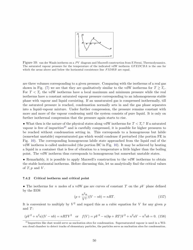
Notes for Thermal Physics course, CMI, Autumn 2019 Govind S. Krishnaswami, November 19, 2019 These lecture notes are very sketchy and are no substitute for books, attendance and taking notes at lectures. More information will be given on the course web site http://www.cmi.ac.in/ ~ govind/teaching/thermo-o19. Please let me know (via [email protected]) of any comments or corrections. Help from Sonakshi Sachdev in preparing these notes is gratefully acknowledged. Contents 1 Thermodynamic systems and states 1 1.1 Thermodynamic state of a gas and a paramagnet .......................................... 2 1.2 Thermodynamic processes ....................................................... 4 1.3 Work .................................................................. 6 1.4 Exact and inexact differentials .................................................... 7 1.5 Ideal gas laws ............................................................. 9 2 Heat transferred and the first law of thermodynamics 12 2.1 Heat transferred and its mechanical equivalent ............................................ 12 2.2 First Law of Thermodynamics .................................................... 13 2.3 First law for systems with ( p, V, T ) state space, three δQ equations and specific heats ...................... 14 2.4 First law for paramagnet ....................................................... 15 3 Applications of the first law 15 3.1 Gay-Lussac and Joule experiment: irreversible adiabatic expansion ................................. 15 3.2 Joule-Kelvin (or Joule-Thomson) porous plug experiment and enthalpy .............................. 16 3.3 Heat capacities of ideal gases ..................................................... 17 3.4 Mayer’s cycle for mechanical equivalent of heat ........................................... 18 3.5 Adiabatic transformation of an ideal gas ............................................... 19 3.6 Pressure and temperature in the atmosphere ............................................. 19 3.7 Carnot Cycle .............................................................. 20 4 Second law of thermodynamics 22 4.1 Kelvin and Clausius postulates and their equivalence ........................................ 22 4.2 Consequences of the 2nd law for efficiency of engines ........................................ 23 4.3 Absolute thermodynamic temperature ................................................ 24 4.4 Equality of absolute thermodynamic and gas temperatures ..................................... 26 4.5 Clausius’ Theorem ........................................................... 26 5 Entropy and some consequences of the 2nd law 28 5.1 Absolute temperature as an integrating denominator and the entropy ............................... 28 5.2 Exactness of dS = δQ/T and the energy equations ......................................... 29 5.3 Entropy of an ideal gas ........................................................ 30 5.4 Properties of entropy and examples .................................................. 31 5.5 Boltzmann’s statistical interpretation of entropy ........................................... 34 5.6 Thermal expansion, compressibility and tension coefficients for an ideal gas ............................ 35 6 Thermodynamic potentials 36 6.1 Legendre transform from internal to free energies and enthalpy ................................... 36 6.2 Interpretation of Helmholtz free energy ................................................ 38 6.3 Gibbs’ criteria for thermodynamic equilibrium ............................................ 39 6.4 Maxwell relations ........................................................... 40 6.5 Extensivity, Euler equation and Gibbs-Duhem relation ....................................... 41 7 Phase transitions 42 7.1 General features of 1st and 2nd order transitions .......................................... 42 1
Transcript
Notes for Thermal Physics course, CMI, Autumn 2019Govind S. Krishnaswami, November 19, 2019
These lecture notes are very sketchy and are no substitute for books, attendance and taking notes at lectures. More information will begiven on the course web site http://www.cmi.ac.in/~govind/teaching/thermo-o19. Please let me know (via [email protected]) of any comments orcorrections. Help from Sonakshi Sachdev in preparing these notes is gratefully acknowledged.
Contents
1 Thermodynamic systems and states 1
1.1 Thermodynamic state of a gas and a paramagnet . . . . . . . . . . . . . . . . . . . . . . . . . . . . . . . . . . . . . . . . . . 2
• Thermodynamics arose in part from the needs of steam engine builders; the need to under-stand the possibility and limits of conversion of mechanical/electrical/chemical energy into heatand vice versa; the attempts to optimize efficiencies of heat engines and refrigerators etc. An im-portant role was played by the study of the behavior of gases and of the heats released/absorbedin chemical reactions. Another motivation came from the remarkable phenomena discovered inphase transitions such as the boiling or freezing of water.
• Before discussing the state of a thermodynamic system, let us recall the concept of thedynamical state of a mechanical system. The state of a mechanical system of point particles isspecified by giving the positions and momenta of all the particles at an instant of time.
• The state variables of a thermodynamic system depend on the sort of system it is. Someexamples of thermodynamic systems include gases and liquids (fluids), solids, magnets, chemi-cal solutions, electrolytes, blackbody radiation, stars, black holes etc. These systems typicallycontain a very large number of microscopic constituents and it would be impractical to followtheir individual motions. What is more, in most cases, the thermodynamic understanding haspreceded a detailed understanding of the nature of microscopic degrees of freedom. Thus, ther-modynamics deals with ‘macroscopic’ properties of these systems without reference to positionsand momenta of constituents. As opposed to the dynamical state of a gas of N molecules, whichwould be specified by N positions and momenta, the thermodynamic state is defined by just ahandful of state variables (a number independent of N ).
• Perhaps the simplest thermodynamic system is a homogeneous gas (or fluid) composed of asingle chemical substance (e.g. oxygen or water) at rest (no flow). Volume, constant pressureand density are obvious mechanical properties associated with the uniform fluid. In addition tomechanical properties, thermodynamics deals with the temperature of the gas, which may bemeasured with, say, a mercury thermometer1. For the present we use the same thermometer forall temperature measurements to make them comparable.
• Thus, thermodynamics postulates the existence of temperature as a thermal propertyof a system. It is a parameter of state being defined by the instantaneous state of the systemindependent of its history.
1Operationally, we have a column of mercury of height h at some reference temperature (say freezing pointof water at atmospheric pressure). We say that the water freezes at temperature h . When heated, the mercuryexpands and the temperature is defined simply to be the height of the column.
2
• It is observed that a fluid when left to itself (‘isolated’) for some time settles into a state ofthermal equilibrium, characterized by a common temperature everywhere. Thus the zeroth lawof thermodynamics postulates that parts of a system (or different systems) are in thermalequilibrium if they have the same temperature. Furthermore, if system A is in thermal equilib-rium with system B and B is in equilibrium with C then A is in equilibrium with C: all threehave a common temperature. A consequence of this transitivity is that it allows us to concludethat a bar of iron and a bucket of water are in thermal equilibrium even without bringing theminto contact, provided we check that each is separately in equilibrium with a third system, whichplays the role of a thermometer.
1.1 Thermodynamic state of a gas and a paramagnet
• Thermodynamic state of a homogeneous fluid. For the purposes of thermodynamics, auniform fluid has one mechanical degree of freedom, its volume. It is found that thermodynamicproperties (like energy) are largely independent of the shape of the region occupied by the fluidas long as its volume is large (compared to molecular dimensions) and surface area not too largecompared to that of a sphere of the same volume. This is not true for microscopic volumes norfor regions with very large surface area like the small intestine - we will exclude such regionsfrom this discussion.
• Just as momentum is conjugate to the position of a particle in mechanics, we will see thatpressure is the variable conjugate to volume2. The thermodynamic state of a fixed mass ofhomogeneous fluid is fixed once the volume V , the (uniform) pressure p and temperature thave been specified. Thus, the thermodynamic state space is three dimensional. However, notall triples (V, p, t) represent equilibrium states. Equilibrium states have the special propertyof remaining unchanged in time under fixed external conditions. For instance, a flowing gas isnot in equilibrium (at the very least, one would need to specify the velocity and pressure atdifferent locations in the gas to determine its state). Equilibrium states lie on a 2D surface(called the equilibrium manifold) determined by a relation f(V, p, t) = 0 called the equation ofstate. The equation of state allows us to express one of the state variables, say p(V, t), as afunction of the other two. We will see that for many dilute gases at sufficiently high temperaturesand low pressures (ideal gases) the equation of state is approximately pV = nRT where theproportionality constant nR is the product of the number of moles of gas (amount of substance)and the universal gas constant and T is the so-called gas thermometer temperature (to beintroduced later).
• Following James Watt, the state of such a gas can conveniently be represented by a point inthe V -p plane (indicator diagram) with abscissa V along the horizontal axis and ordinate palong the vertical axis. An isotherm is a curve along which temperature is constant. A PT -diagram is sometimes convenient especially when studying phase transitions, say between liquidand vapour.
• The first derivatives of p, V, T with respect to each other are used to define three material
2Hydrostatic pressure at a point A is introduced as follows: Consider a small fictitious membrane (flat surface)passing through A in a gas/fluid. It is found that the fluid on one side of the membrane exerts a force normalto the membrane and towards the other side. This normal force per unit area is the hydrostatic pressure. Thesame value of pressure is obtained by considering the normal force per unit area due to the fluid on the otherside. Moreover, the value of pressure at a point is independent of the orientation of the membrane through thepoint: it is a positive scalar quantity.
3
properties which describe the response of one due to a change in another keeping the thirdfixed. Thus we have the coefficients of thermal expansion, thermal tension3 and isothermalcompressibility
α =1
V
(∂V
∂T
)p
, β =1
p
(∂p
∂T
)V
, κT = − 1
V
(∂V
∂p
)T
. (1)
For instance, compressibility κT measures the fractional change in volume of a gas due to anincrease in pressure. The minus sign is because gases are compressed upon the application ofpressure. The reciprocal of compressibility is called the bulk modulus. There are three moresuch coefficients that we could define, involving ∂T
∂V , ∂T∂p and ∂p
∂V . However, we will see that onthe equilibrium surface, there are four relations among these six coefficients so that only two canbe independent. Let us also note that the coefficients α, β and κ are in general not constantand vary from place to place on the equilibrium manifold.
• The fact that p, V and T satisfy the equation of state leads to the relations(∂p
∂V
)T
=
(∂V
∂p
)T
,
(∂T
∂p
)V
=
(∂p
∂T
)V
and
(∂V
∂T
)p
=
(∂T
∂V
)p
(2)
as well as the remarkable relation among the three coefficients α, β and κT .
p β κT = α. (3)
This is obtained by replacing x, y, z by p, V, T in the identities we now derive.
• In general, if x, y, z satisfy a functional relation f(x, y, z) = 0 that allows us to locally express eachas a function of the other two z = z(x, y), y = y(z, x) and x = x(y, z), then we have the ‘triple product’identity4 (
∂z
∂x
)y
(∂x
∂y
)z
(∂y
∂z
)x
= −1 (4)
that holds on the constraint surface f(x, y, z) = 0. To see this we write the differentials with subscriptsdenoting partial derivatives (E.g. zx =
(∂z∂x
)y
, the variable that is held fixed in the partial derivative is
not indicated explicitly as it is clear from the context)
dz = zx dx+ zy dy, dx = xy dy + xz dz, and dy = yz dz + yx dx. (5)
Now we regard x and y as independent variables on the constraint surface & write dz in terms of dx &dy in the formula for dx
dx = xy dy + xz (zx dx+ zy dy) . (6)
Since dx and dy are independent differentials on the 2d surface f = 0, their coefficients must vanish.
The coefficient of dx vanishes provided xzzx = 1 (i.e.,(∂x∂z
)y
(∂z∂x
)y
= 1). Since we could equally well
have taken any other pair as independent variables, we must also have xyyx = yzzy = 1. Now requiring
that the coefficient of dy vanish gives xzzy = −xy which becomes zxxyyz = −1 upon using the previous
result.
• Thermodynamic variables can often be classified as extensive or intensive. Extensivequantities are proportional to the amount of material. For example, internal energy (U ), the
3Tension is another word for force and thermal tension refers to the change in pressure (force/area) as tem-perature is varied.
4To remember this formula, begin with any of the partial derivatives as the first factor. The latter two factorsare obtained by cyclically permuting the variables in the first partial derivative.
4
various free energies (e.g. Helmholtz free energy F ) and entropy (S ) are extensive variables,they scale with the volume V (ignoring boundary/surface effects), the number N of particlespresent or the total mass m . By dividing by N , V or m we obtain the corresponding ‘specific’energies or entropy. Intensive quantities such as pressure, temperature and chemical potential(to be introduced later) are independent of the amount of substance. We will see that (p, V ),(µ,N) and (t, S) are canonically conjugate pairs of intensive and extensive variables.
• Magnets as thermodynamic systems: The analogs of pressure and volume for a magneticmaterial are the external magnetic field (H , intensive) and magnetization (M , by conventiondipole moment per unit volume, intensive). A ferromagnet such as an iron bar magnet (a‘magnetic dipole’) has a permanent magnetization (pointing, say, in the z direction). Themagnetization leads to a magnetic field in the neighbourhood of the magnet, which aligns ironfilings. By measuring the magnetic field, one can infer the magnetization. The magnetizationof a ferromaget is permanent (more precisely spontaneous) in that it is non-zero even in theabsence of an external magnetic field. From a microscopic viewpoint, the magnetization is thevector sum of molecular magnetic moments per unit volume. A paramagnetic substance has nomagnetization of its own since thermal fluctuations ensure that the molecular magnetic momentspoint in random directions and sum to zero. However, in the presence of an external magneticfield H , it acquires a magnetization M that points along H . Ferromagnets gradually lose theirspontaneous magnetization with increase in temperature. The spontaneous magnetization dropsto zero above the Curie temperature tc (770 Celsius for iron) and then ferromagnets becomeparamagnets. This is a phase transition which bears some resemblance to the liquid to gasvapourization transition. By convention, we will assume that H , and therefore M , point in thez -direction and denote them by their z -components H and M . Thus, the thermodynamic statespace of a uniformly magnetized homogeneous paramagnet is three dimensional with coordinatesH,M and t . H and M are conjugate variables like the pressure and specific volume (volumeper particle) of a gas. In equilibrium, there is an equation of state that relates H,M and t .For a linear paramagnetic medium M = χH where M is the magnetization per unit volume(V the volume of the magnet is essentially a constant, unlike for a gas). This simply statesthat the induced magnetization is proportional to the applied magnetic field. The magneticsusceptibility χ depends on temperature, it is a measure of how ‘magnetizable’ a paramagnetis. At high temperatures (t > tc ) the paramagnetic susceptibility is given approximately bythe Curie-Weiss5 law χ ≈ C/(t− tc) for an appropriate temperature scale. C is called Curie’sconstant.
1.2 Thermodynamic processes
• A process is a transformation of a system from an initial state through a continuous successionof intermediate states to a final state. It may sometimes be represented by a curve in thethermodynamic state space, in which case we could call it a thermodynamic process (this maynot be possible if the transformation produced inhomogeneities so that, say, the pressure is notconstant throughout). A transformation in which the system is always infinitesimally close toan equilibriums state is called a reversible or quasi-static transformation. For a homogeneousgas, such a process may be represented by a curve that lies entirely on the equilibrium surfacein the p-V -t state space; it may also be represented by a curve in a p-V diagram. Starting
5Named after the Polish-French and French physicists Marie Curie and Pierre Weiss.
5
Figure 1: From K Huang, Introduction to statistical physics: V, p, t thermodynamic state spaceof a gas of uniform composition. Reversible processes are curves on the equilibrium EOS surface.Irreversible processes which can be represented in such a diagram go off the equilibrium surface.
from an equilibrium state, a reversible transformation may be realized through a slow variationof external conditions so that the system always has time to adjust itself to the new equilibriumstate corresponding to the altered conditions6. For example, the slow expansion of a gas in acontainer fitted with a piston (that can move vertically), as small weights are slowly removedfrom the piston and kept aside at the same height. The process may be reversed by replacing theweights onto the piston slowly as the gas contracts. If the piston is lowered rapidly, the pressurewould not be uniform and there would also be velocity currents set up in the gas, making it passthrough non-equilibrium states. A transformation passing through equilibrium states from A toB is called reversible since it can be reversed by applying the changes to the external conditionsslowly in the opposite order, so that the system passes through the same intermediate statesbut from B to A .
• A process that is not reversible (not quasi-static) is called irreversible. Irreversible processesmay not always be representable as curves in the pV t state space, since we may need to specifyother variables like velocity and there may not be a single pressure that can be assigned to thewhole gas.
• Note that a slow process need not be reversible. Examples may be found among dissipativeprocesses such as the slow frictional heating of the suspension of a swing as it executes dampedoscillations or the slow heating of a resistor connected to a battery. Even if we try to reversethese processes (by reversing the direction of oscillation of the swing or reversing the directionof current) heat is still produced, not absorbed!
• The spontaneous flow of heat (whether quickly or slowly) from a body at a higher temperatureto one at a lower temperature is irreversible. Indeed, we do not see heat spontaneously flowingfrom a cold body to a hot one.
• Thermodynamic processes in which p, V or T remain constant are called isobaric, isochoric(isopiestic) and isothermal.
• A cycle or cyclic process is a transformation in which the initial and final states are the same.On a p-V diagram, a cycle is represented by a closed curve (which could have self-intersections).
6In other words, for the purposes of the thermodynamic process, we only observe the system at intervals oftime that are large compared to the equilibration time of the system. So the ‘continuity’ of the process needs to beunderstood in this sense. We will not attempt to understand the dynamical process of how the system approachesequilibrium: this lies outside the purview of thermodynamics and requires a kinetic or dynamical treatment.
6
Figure 2: From A Sommerfeld, Thermodynamics and Statistical mechanics: pV diagram for a cycle of a steamengine. Work done is equal to shaded area enclosed and is positive as the curve runs clockwise. The isobar at thehigh pressure p1 corresponds to the steam in the cylinder expanding while in contact with the boiler. The isobarat the low pressure p2 corresponds to compression when in contact with the atmosphere or condenser.
Cyclic processes are important in practical applications as they can be repeated, as in a steamengine or refrigerator. Cyclic processes are also of great conceptual value, as we will learn.
1.3 Work
When a gas expands, it does work ∆W on the surroundings; the surroundings do work −∆Won the system. Our convention is to take the work done by the gas as positive in the case ofan expansion and negative in the case of a contraction. More generally, a system can performwork (mechanical - movement of a piston, electrical/chemical - movement of charges/ions in anelectric potential etc.) during a thermodynamic process. For example, consider a gas enclosedin a cylinder with a movable piston of area A . If p is the uniform pressure in the gas, theforce exerted on the piston is pA . If the piston moves out a distance ∆l , the work done is∆W = pA∆l . In general, if the volume of a gas increases by dV in an infinitesimal expansion,then the work done by the gas is δW = pdV . This can be shown by breaking up the boundingsurface into small pieces and treating each as a small piston.
• Suppose the state can be represented on a p-V diagram, then a transformation from state(Va, pa) to (Vb, pb) is represented by an oriented curve γa→b joining these points. The work done
W (γ) =∫ ba pdV is given by the area under the curve (see figure). Note that the pressure could
change during the process and that the area can be negative, as in a compression (Vb < Va ). Inparticular, the work done in a cycle (represented in a p-V diagram) is the area enclosed by thecurve. For a simple closed curve, the area is positive if traversed clockwise and vice-versa. dVand δW both vanish in an infinitesimal isochoric transformation.
• In electromagnetic theory it is shown that the work done by the external field H in increasingthe magnetization of a paramagnet from M to M+dM is µ0HdM where µ0 is the permeabilityconstant. Thus, the work done by a magnet in the process is δW = −µ0HdM . Up to a sign,this is analogous to δW = pdV for the work done by a gas.
• It is very important to recognize the empirical fact that the work done during a process γa→bin general depends on the process and not just on the initial and final states. For example,consider initial and final equilibrium states of water at temperatures ta and tb > ta , but at acommon pressure, say atmospheric pressure. The corresponding volumes are determined by theequation of state. Now, we can go from state a to b in more ways than one. For instance, wecould vigorously stir the liquid for some time and heat it up through friction, thereby doinga significant amount of work (this work is not calculable by integrating ‘pdV ’ since in the
7
intermediate stages, we would have set up a velocity field in the water and we would have toevaluate the work done in setting up the flow etc.). Alternatively, we could simply heat theliquid using a flame, in which case hardly any work is done (the liquid does a little work inexpanding against atmospheric pressure). Both these processes are irreversible, but the first oneinvolves a lot more work.
• This path-dependence of the work done is reflected in the fact that areas under differentcurves joining a to b in a pV diagram are not necessarily the same. In other words, unliketemperature, there is no ‘work function’ or property of state W such that W (b) − W (a) isthe work done during the process. In particular, the work done in an infinitesimal process δWdepends on external effects and is not the differential of any state function W . This is why wedo not denote it ‘dW ’. We say that the work done in an infinitesimal process is not an exactdifferential.
1.4 Exact and inexact differentials
Two independent variables: Given a differentiable function, say of two variables σ(x, y), itsdifferential is dσ = ∂σ
∂x dx+ ∂σ∂y dy . Under suitable hypotheses (it suffices for σ to have continuous
second partial derivatives), the ‘mixed’ second partials are equal: ∂2σ∂x∂y = ∂2σ
∂y∂x . This is calledSchwarz’s or Clairaut’s theorem.
• On the other hand, suppose we are given a differential expression (also known as a one-form orPfaffian differential) ω = f(x, y)dx+g(x, y)dy on the plane. We ask whether ω is the differentialof some function σ , i.e., is ω = dσ? σ would in a sense be an ‘integral’ of ω and we would callω a perfect or exact differential. A necessary condition for this (it is also a sufficient conditionon the plane - this is Poincare’s lemma) follows from the above remark: f and g must satisfy∂f∂y = ∂g
∂x . This is called the integrability condition for ω to be exact: if it is satisfied, we can‘integrate’ ω to find σ . If we use the components of ω to define a ‘coefficient’ vector fieldv = (f, g) = fx + gy on the plane, this integrability condition states that v must be curl free∇× v = (gx − fy)z = 0. Here, we use subscripts to denote partial derivatives.
• The curl of a vector field measures how much the vector field circulates or swirls around. In3d if v = (f, g, h) then ∇ × v = (hy − gz, fz − hx, gx − fy). The curl of a vector field on aplane points normal to the plane since h = 0 while f and g are independent of z . An exampleof a curl-free planar vector field is v = xx + yy . It points radially outwards. The integrabilitycondition is satisfied and indeed we see that σ = (x2 + y2)/2 is a function whose differentialequals ω = xdx+ ydy . On the other hand ω = −ydx+xdy is not exact since it does not satisfythe integrability condition and the corresponding vector field v = −yx+ xy has non-vanishingcurl: v it points azimuthally and describing swirling motion counterclockwise around the origin.
• In passing, we note that given a vector field v = (f, g, h) we can define another derivative,namely its divergence, which is a scalar ∇·v = fx+gy+hz . The divergence measures expansion orcompression and can sometimes be associated with the presence of sources or sinks. For instancev = (xx + yy) has divergence ∇ · v = 2 but no curl. However, the integrability condition forexactness is not related to the divergence of the coefficient vector field.
• There is a third notion of derivative, namely the gradient which takes a function σ(x, y, z)and produces a vector field ∇σ = σxx + σyy + σz z . Our statement on the exactness of ω canthen be restated as follows: ω is exact (ω = dσ) if the coefficient vector field v is curl-free and
8
in that case, v = ∇σ is the gradient of the scalar function σ .
• In the last section we asserted that the work differential (work that can be done by a gas in aninfinitesimal expansion) δW = pdV is not exact in general. As another example, consider thePfaffian differential ω = CdT + nRT
V dV in the variables T and V . Here n and R are constantswhile C is independent of V . The above integrability condition is not satisfied since nR/Vis not identically zero. Interestingly, notice that ω/T is an exact differential, the integrabilitycondition is satisfied and we can integrate it to find a function σ such that dσ = ω . Indeedω/T = CdT/T + nRdV/V = d(C log T + nR log V + σ0) ≡ dσ . Notice that σ is defined onlyup to an additive constant. T is called an integrating factor or integrating denominator for theinexact differential ω . More on this later.
• Now if ω is an exact differential, then its line integral between a pair of points a,b on theplane is independent of the path γ connecting them. Indeed, let the path γ : [ta, tb] → R2 begiven by r(t) = (x(t), y(t)) with r(ta) = a and r(tb) = b . Then the tangent vector to the curveis r(t) and the line element dl = r(t)dt and∫
γ
ω =
∫γ
fdx+gdy =
∫γ
v·dl =
∫ tb
ta
(fx+gy)dt =
∫ tb
ta
(σxx+σy y)dt =
∫ tb
ta
dσ(r(t))
dtdt = σ(r(tb))−σ(r(ta)). (7)
The last equality follows from the fundamental theorem of calculus. Path-independence followssince the line integral depends only on the values of the function σ at the end points. Thus, wearrive at a formula for a function σ(r) whose differential is ω :
σ(r) = σ0 +
∫γω (8)
where γ is any curve that joins an arbitrary reference point r0 to r = (x, y). Notice that σ isnot unique: it is determined up to an additive constant which we have taken as σ0 = σ(r0).
• In particular, the integral of an exact differential around a closed contour C vanishes∮dσ = 0.
This may also be seen by an application of Green’s theorem (2d version of Stokes’ theorem)∮Cfdx+ gdy =
∫S
(gx − fy) dxdy = 0 or
∮C
v · dl =
∫S
(∇× v) · z dxdy = 0. (9)
Here S is the two-dimensional region bounded by the closed curve C . Conversely, a differentialω whose line integral around every closed curve vanishes is an exact differential. This is easy toshow, since the function
σγ(x, y) = σ0 +
∫γω (10)
where γ is any curve from an arbitrary reference point (x0, y0) to (x, y) satisfies dσ = ω andis is seen to be independent of the choice of γ . Indeed, the difference σγ − σγ′ for two curvesjoining the same points is equal to the line integral of the exact differential ω around the closedcurve γ ∪ γ′ and therefore vanishes ( γ′ is the curve γ′ traversed in the opposite direction).
Three independent variables: The above statements have a natural generalization to 3D.The differential ω = fdx+ gdy + hdz is locally exact provided the first partials of f , g and hsatisfy
fy = gx, gz = hy and hx = fz. (11)
Here, for instance, fy =(∂f∂y
)x,z
is the partial derivative with respect to y holding x and
z fixed. These three conditions simply state that the coefficient vector field v = (f, g, h, ) is
So, when v is curl-free, we may express it as the gradient of a scalar v = ∇σ or ω = dσ .Furthermore, the line integral
∫ ba ω of the exact differential ω is the difference in values σ(b)−
σ(a) independent of the path.
• The above result can also be obtained from Stokes’ theorem in three dimensions. Given asufficiently smooth vector field v in a simply connected region, its line integral around a closedcurve C can be re-expressed as the surface integral of its curl over any surface S in the regionwhose boundary is C : ∮
Cv · dl =
∫S
(∇× v) · dS. (13)
Now if v is curl-free, the RHS vanishes, so that its line integral around any (necessarily) con-tractible closed path vanishes.
1.5 Ideal gas laws
• It is empirically found that many gases in equilibrium satisfy certain common (‘ideal’ gas)laws at temperatures much higher than their condensation point and at low pressures. At 20 Cand atmospheric pressure of one Atm (or 760 mm of Hg or 760 torr), helium, hydrogen, oxygen,carbon dioxide and air to a reasonable approximation behave ideally while water vapour (steam)does not. An ideal gas is what we would get when we expand a real gas to very large volumes.From the molecular standpoint, an ideal gas is one whose molecules are point-like (i.e. occupynegligible volume compared to that of the container) and do not interact with each other (exertnegligible forces).
• Boyle’s and Mariotte’s Law (1658, 1676): For a given mass of a gas at a fixed tem-perature, the product of pressure and volume occupied by the gas in equilibrium is a constant:p(i)V (i) = Θ(i)(t,m). Based on the investigations of Boyle and Mariotte, the constant Θ(i)(t,m)could depend (and in fact does depend) on temperature t , mass m of gas and on the chemicalnature of the gas (indicated by the species label i).
• Gas temperature scale: By a gas thermometer, we mean the following. We select aspecified volume (say 1 cc) of a gas (such as Helium) that is far from condensation at a referencetemperature (say the freezing point of water at atmospheric pressure of 1 atm). As noted,gases are observed to expand on heating and contract on cooling. We simply define the gastemperature T to be a constant multiple of the volume, with the pressure being held fixed. Theconstant is often fixed by requiring the difference in gas temperatures at the boiling and freezingpoints of water to be 100 at atmospheric pressure. Note that fixing the constant through sucha specification also removes the dependence on the volume of gas we started with, it could havebeen 100 cc instead of 1 cc. It is a remarkable empirical fact (see also the Charles-Dalton-Gay-Lussac law below) that a wide variety of gas thermometers (with different gases, but all of whichhave the same volume at the reference temperature and pressure) agree on their assignment ofgas temperatures as long as the gases are far from condensing. The temperature scale T definedthis way is called the gas thermometer scale (or absolute gas temperature) or the Kelvin scale.Water freezes at 1 atm pressure at T = 273.16 Kelvin. By construction T > 0 since the volumeof a gas is a positive number.
10
• Charles’, Dalton’s and Gay-Lussac’s Law (1787, 1802): (See N D Hari Dass, Theprinciples of thermodynamics) All gases, whatever may be their density and the quantity of waterwhich they hold in solution, and all vapours expand equally between the same degrees of heat.Here ‘same degrees of heat’ means ‘between the same initial and final temperatures’ (freezingand boiling points tf , tb of water at atmospheric pressure in Gay-Lussac’s experiments). By‘expand equally’ he apparently meant the change in volume as a fraction of original volume wasthe same for all gases. The expansion of all gases was carried out at the same fixed pressure p(atmospheric pressure). If the species of gas is labelled i , we may summarize the law by
V(i)tb− V (i)
tf
V(i)tf
= c(p; tf , tb) (14)
for all gases. In other words, the fractional change in volume is independent of species, butwe have allowed for a dependence on the pressure and initial and final temperatures through
c(p; tf , tb). Note that though the volumes V(i)tb, V
(i)tf
depend on the mass of gas present, the ratioon the left is independent of the mass, since it is found that twice the mass of a gas occupiestwice the volume at a fixed temperature and pressure. So the RHS is also independent of massof gas used.
• Now applying the Boyle-Mariotte law, we get
Θ(i)(tb,m)−Θ(i)(tf ,m)
Θ(i)(tf ,m)= c(p; tf , tb). (15)
The dependence on pressure cancels between numerator and denominator on the LHS since theexpansion is carried out at a fixed pressure. Thus the RHS must be independent of pressure andc = c(tf , tb). Moreover, the RHS is independent of species. The simplest way for the LHS tobe independent of species is for Θ(i)(t,m) to be species independent. However, this contradictsexperiment: putting this in Boyle’s law, we would find that the product pV for mass m of anygas is the same function of temperature Θ(t,m). However, it is found that a common mass m ofdifferent gases at the same temperature have different constant values for the product pV . Thisis also why in setting up the gas thermometer, we did not take equal masses of different gasesbut rather equal volumes at a common temperature and pressure. The next simplest possibilityis that Θ(i)(t,m) = ν(i)(m) Θ(t) is the product of a species-dependent function ν(i)(m) and aspecies-independent function of temperature. The constant ν(i)(m) cancels in the quotient onthe LHS of (15), ensuring that the RHS is independent of both i and m .
Putting this in the Boyle-Mariotte law, we deduce that for a fixed mass m of any gas (labeledi) at a fixed temperature t ,
p(i)V (i) = ν(i)(m) Θ(t). (16)
Here Θ(t) is a universal function of temperature. Now we are free to choose our temperaturescale. The law takes its simplest form when we use the gas thermometer scale of temperature,in which case Θ(T ) is a universal constant multiple, say R , of T (since we defined the gasthermometer temperature to be a multiple of the volume of the gas holding p,m fixed). Thusthe simplest way of satisfying the observations of Boyle-Mariotte-Charles-Dalton-Gay-Lussac isfor gases to obey
p(i)V (i) = ν(i)(m) RT (17)
11
where T is the gas thermometer temperature. As we will see, ν(i)(m) depend on the speciesvia a characteristic property which we now recognize as their molecular masses. This brings usto Avogadro’s postulate.
• Avogadro’s postulate (1811): Equal volumes of all gases at the same temperature andpressure have the same number of corpuscles (molecules), but (in general) different masses.However, the molecular constitution of matter took nearly a century to be confirmed. In theinterim, it made sense to reformulate Avogadro’s postulate in terms of measurable quantities.Ostwald introduced the concept of moles for this purpose. A gram-mole or gram molar massµ of a gas was defined as a definite number of grams of a gas. For example, one gram-mole ofhydrogen is 2 grams of the gas (i.e. µ = 2 for H2 ). A gram mole of oxygen is 32 grams (i.e.µ = 32 for O2 ).
• These assignments were based on the proportions in which elements combined to form chemicalcompounds (the subject of Dalton’s and Gay-Lussac’s laws of multiple proportions7 and integralvolume ratios8), but could also be deduced from calibrating gas thermometers with the samemass of different gases with each other. In current language, one gram mole of a compoundis as many grams as there are units in the sum of atomic weights of the constituent elements,with the Hydrogen atom being assigned an atomic weight of one since it is the lightest knownelement. We often refer to one gram mole of a gas as simply one mole of the gas. Avogadro’slaw in Ostwald’s formulation states that equal volumes of all gases at a common pressure andtemperature contain equal numbers of moles of the gas. So suppose we consider one gram-moleof gas i (i.e. µi grams) as well as one gram mole of gas j (i.e. µj grams) at the same pressureand temperature. The Avogadro-Ostwald postulate along with the Boyle-Mariotte-Gay-Lussac-Charles law implies
V (i) = V (j) orν(i)(µi)RT
p=ν(j)(µj)RT
por ν(i)(µi) = ν(j)(µj) ∀ i, j. (18)
Thus the constants ν(i)(µi) are independent of species if we consider one gram mole of eachspecies. We can take this universal constant to be one, by a rescaling of R . Thus, for one moleof an ideal gas, pV = RT . If we had considered n gram moles instead of one gram mole, thevolume occupied at a fixed temperature and pressure is found to be multiplied by n , so we arriveat pV = nRT for n gram moles of any sufficiently ideal gas. In other words, ν(i)(m) = m/µi .To see this, we first note by the property just noted that ν(i)(m) ∝ m is proportional to themass of the gas, so for some proportionality constant ki (depending on species),
ν(i)(m) = ki m. (19)
Taking one gram mole of gas i we have m = µi . Now, using our observation that
ν(i)(µi) = 1 we get kiµi = 1 or ki =1
µi. (20)
7Dalton’s law of multiple proportions: When two elements combine with each other to form more thanone compound, the masses of one element that combine with a fixed mass of the other are in a ratio of small wholenumbers. E.g. 24g of carbon combine with 32g of oxygen to form 56g of carbon monoxide. 24g of C alsocombine with 64g of oxygen to give 88g of carbon dioxide. So the ratio of oxygen masses that combinewith the same mass of carbon is 1 : 2 .
8Gay-Lussac’s law of integral volume ratios: The ratio between the volumes of the reactant gases andthe products can be expressed in simple whole numbers. E.g. 4g of hydrogen gas combine with 32g of oxygento give 36g of water vapour. It is found that two litres of hydrogen combines with one litre of oxygen togive 2 litres of water vapour. The ratio of volumes of reactants to product is 3 : 2 .
12
• Ideal gas law: Combining Avogadro’s postulate with the Boyle-Mariotte and Charles-Dalton-Gay-Lussac laws in the manner above, it is found that the equation of state of an ideal gas takesa particularly simple form when we use the gas thermometer scale. For m grams of a gas withgram molecular mass9 µ ,
pV = (m/µ)RT. (21)
• Here R = 8.314 Joules/Kelvin per mole is the universal gas constant. From Ostwald’sdefinition, the quotient n = m/µ is the number of moles of the gas. By Avogadro’s law, onemole of all (nearly ideal) gases contain the same number of molecules, namely NA = 6.023×10²³
(Avogadro’s number, estimated by J J Loschmidt in 1856 and more accurately measured by JB Perrin in 1909 after Einstein’s work on Brownian motion).
• The ideal gas EOS may also be expressed as a relation among pressure, density ρ = m/V andtemperature p = ρRT/µ . Alternative forms are pV = nRT and pV = NkBT where N = NAnis the number of molecules and kB = R/NA = 1.38× 10⁻²³ J/K is Boltzmann’s constant. If weintroduce the specific volume v = V/m which is the reciprocal of density, then the ideal gas lawstates that pv = RT/µ .
• As noted, from a microscopic viewpoint, an ideal gas is a collection of molecules of a givenchemical species occupying a volume much larger than the size of the molecules and whoseinter-molecular forces can be ignored. The Hamiltonian for such a collection of molecules is thesum (1/2M)
∑a(p
2a) where the various molecules are labelled by a and M is the mass of each
molecule. It is not surprising, then, that all gases that can be approximated by such a treatmentbehave in the same way except for the difference in the masses of the molecules. The molecularmass enters the ideal gas law through µ (M = µ/NA ) and is the only way in which the gasmanifests its chemical identity.
• For an isothermal transformation of a fixed amount of an ideal gas, pV is a constant. Thus, ona p-V diagram, an isotherm is represented by a hyperbola with the p and V axes as asymptotes.The work done by the gas in a reversible isothermal expansion from volume V1 to V2 is
W =
∫ V2
V1
p(V )dV = nRT
∫ V2
V1
dV
V= nRT log(V2/V1) = nRT log(p1/p2). (22)
2 Heat transferred and the first law of thermodynamics
2.1 Heat transferred and its mechanical equivalent
• Caloric theory of heat: Prior to the mid 1800s heat was regarded as a substance, the‘caloric’ which was thought to be like a fluid that flowed while its amount was conserved10. Thisis in contrast to the current view that heat is a form of energy that can be transformed (partly)into (or arise from) other forms of energy. The heating of water by a flame was assumed to involveflow of the caloric (heat-fluid) from the fire to the water. When a bottle of hot water was broughtinto contact with a bottle of cold water, it was supposed that the heat fluid flowed from hotto cold water till the temperatures were equalized. The theory was not without merit. Carnot(1824) correctly deduced limits to the conversion of heat into work based on the caloric theory.
9For example, the gram molecular mass of H2 molecule is 2 while that of that of He42 atom is 4.
10An even earlier (now discarded) theory of combustion was the Phlogiston theory, developed from 1667 onwards.
13
However, the caloric theory had to be replaced since it contradicted experiment. The amountof heat fluid was not conserved: heat could be produced entirely from mechanical or electricalwork, as in the heating of a resistor/filament of a light bulb or the melting of two pieces of icewhen rubbed together. The caloric theory of heat was replaced by a more mechanical theory ofheat.
• The amount of heat transferred in a process may be quantified through temperature mea-surements. One calorie of heat transferred is defined as the quantity of heat required toraise the temperature of one gram of water from 14 to 15 C at atmospheric pressure. Itis important to recognize that while we can measure and define the heat exchanged betweensystems, we have not defined the ‘heat content’ of a system.
• Mechanical equivalent of heat Count Rumford (also known as Benjamin Thompson, 1798)famously demonstrated that water could be made to boil while the shaft of a canon was beingmechanically bored. Water could also be heated through stirring using immersed paddles thatwere made to rotate by letting a weight descend under gravity. Several careful experimentsshowed that the heat transferred (in calories) was proportional to the work done (say in Joulesor ergs), through a universal proportionality constant δQ = (1/J)δW . Precisely, to transfer onecalorie of heat, the same amount of work, i.e. J = 4.186 Joules had to be done. Thus 4.186Joules of work done is the mechanical equivalent of one calorie of heat transferred.
2.2 First Law of Thermodynamics
• In 1842 Robert Mayer presented a mechanical theory of heat, based on the transformability ofheat into mechanical energy (and vice versa), and formulated the 1st law of thermodynamics. Wewill state the first law and later describe the cyclic process he used to determine the mechanicalequivalent of heat. A similar process had been considered by Sadi Carnot somewhat earlier.Hermann Helmholtz (1847) made Mayer’s ideas on the first law mathematically more precise.The first law was the work of these and several other scientists.
• The first law postulates the existence of the internal energy as a state function of a thermo-dynamic system. It posits that the heat added to a system is equal to the sum of the increasein its internal energy (denoted U by Rudolf Clausius) and the work done by the system.
∆Q = ∆U + ∆W. (23)
We may regard the first law as a generalization of the statement of conservation of energy. Foran isolated system (thermally and mechanically/electromagnetically etc), the internal energy isconserved. For a thermally insulated system, the work done by the system is equal to the dropin its internal energy ∆W = −∆U .
• Given the state of a system, we can speak of the internal energy of that state, but not the‘heat content’ or ‘work’ of the system in that state, heat and work are not state functions, theyare measures of external effects. If the caloric theory was true, heat would be a state function,equal to the amount of caloric fluid.
• For a cyclic process, the initial and final states are the same so ∆U = 0 and the 1st lawbecomes ∆Q = ∆W , i.e., the work done is equal to the heat absorbed.
• For an infinitesimal reversible expansion of system volume dV against a pressure p , the work
14
done is δW = pdV . So for infinitesimal reversible processes, we write
δQ = dU + pdV. (24)
Unlike the heat and work differentials δQ and δW which are not exact, the internal energydifferential dU is an exact differential. So for a cyclic process
∮dU = 0. On the other hand,
there is no state function Q such that δQ is equal to dQ .
• The 1st law allows us to measure heat exchanged in energy units. It is found that 1 calorie ofheat exchanged is equivalent to 4.186 Joules of energy.
• The first law is sometimes interpreted as stating the impossibility of constructing a machine(perpetuum mobile or perpetual motion machine of the first kind) that can create or destroyenergy. Rather, energy can be transformed into other forms such as mechanical/electrical workand heat.
• When the number of particles N in the system can change, the internal energy of a systemcould change even if no mechanical work is done on the system nor any heat transferred to it.It is conventional to define the chemical potential µ as the energy required to add one particleto a thermally and mechanically isolated system. The first law is then generalized to
∆Q = dU + ∆W − µ∆N or δQ = dU + pdV − µdN (25)
for an infinitesimal process. We may interpret this equation as saying that the heat added to acup of water by a flame is equal to the sum of the increase in its internal energy, the work thewater does in expanding against atmospheric pressure and the energy lost to particles expelledfrom the container (dN < 0, µ > 0, here N is ).
• Based on the manner they enter the equation for energy conservation, we say that p and Vare conjugate variables as are µ and N . In each pair we have one intensive and one extensivevariable. Notice that the product of conjugate variables has dimensions of energy.
2.3 First law for systems with (p, V, T ) state space, three δQ equations and specific heats
• If the state of a thermodynamic system (such as a homogeneous gas) can be represented by apoint in PV T space (subject to the equation of state), then we may express the state functionU in terms of any one of the three pairs of independent variables. For instance, taking (T, p) asindependent variables, the infinitesimal increase in volume and internal energy are
dV =
(∂V
∂T
)p
dT +
(∂V
∂p
)T
dp and dU =
(∂U
∂T
)p
dT +
(∂U
∂p
)T
dp. (26)
Then the 1st law δQ = dU+pdV implies the following three ‘δQ equations’ for the infinitesimalheat added to a system with the indicated variables taken as independent:
(T, V ) −→ δQ =
(∂U
∂T
)V
dT +
[(∂U
∂V
)T
+ p
]dV,
(T, p) −→ δQ =
[(∂U
∂T
)p
+ p
(∂V
∂T
)p
]dT +
[(∂U
∂p
)T
+ p
(∂V
∂p
)T
]dp,
(p, V ) −→ δQ =
(∂U
∂p
)V
dp+
[(∂U
∂V
)p
+ p
]dV. (27)
15
• We define the heat/thermal capacity of a system as the ratio C = δQ/dT of infinitesimalheat added (usually reversibly) to the consequent increase in temperature. The heat capacitygenerally depends on how the system is heated. Of particular significance are the principal heatcapacities CV , Cp at constant volume and pressure. Taking (T, p) and (T, V ) as independentvariables in (27) we obtain expressions for CV , and Cp in terms of derivatives of state functions
CV =
(∂U
∂T
)V
and Cp =
(∂U
∂T
)p
+ p
(∂V
∂T
)p
=
(∂H
∂T
)p
(28)
We may intuitively argue that Cp should generally exceed CV since at constant pressure, addi-tional heat must be supplied for the gas to do work while expanding while at constant volume,all the heat added goes into increasing the internal energy and temperature.
• Note that CP can also be written as CP = ∂T (U + pV ) where the partial derivative isevaluated at constant pressure. It is therefore natural to introduce the new extensive statefunction ‘enthalpy’ H = U+pV and express Cp as the temperature derivative of H at constantpressure, just as CV is the temperature derivative of U at constant volume. The formulaH = U + pV is reminiscent of the rough formula H = −L+ pq relating the Hamiltonian to theLagrangian in mechanics. More on this analogy later.
• The heat capacities are extensive as U and V are. It is often convenient to define the corre-sponding intensive quantities cV , cp by considering the heat exchanged per unit mass (specificheats) or per mole or molecule (molecular heats).
2.4 First law for paramagnet
Recall that the thermodynamic state space of a paramagnet is three dimensional with coordinatesgiven by external magnetic field H (z component), z -component of magnetization M andtemperature T . From electromagnetic theory, the work done by the external field in increasingthe magnetization from M to M + dM is µ0HdM . Thus the first law takes the form (PaulLangevin, 1905)
δQ = dU − µ0HdM (29)
Comparing with δQ = dU + pdV for a gas, we see that roughly, p and −µ0H play similar roleswhile volume and magnetization are analogous. The equation of state for a paramagnet bearssome resemblance to the ideal gas law. Indeed, comparing the Curie-Weiss law with the idealgas law,
M = χH =CH
(T − Tc)and ρ =
µp
RT, (30)
we see that Curie’s constant C plays the role of µ/R while magnetization (per unit volume)is like density and H is like pressure. T − Tc for the paramagnet is replaced with the gasthermometer temperature.
• As for a gas, we may define heat capacities and specific heats of a paramagnet at constantmagnetic field or constant magnetization. See Haridass or Sommerfeld for further discussion.
3.1 Gay-Lussac and Joule experiment: irreversible adiabatic expansion
• Gay-Lussac (1807) confined a gas in a thermally insulated cylindrical container fitted witha movable piston. Initially, the gas was in equilibrium at temperature T1 , pressure p1 andoccupied volume V1 . The piston was suddenly moved outwards, increasing the available volumeto V2 . The gas expanded (through a complicated flow) and eventually reached equilibriumat a lower pressure p2 in volume V2 . Remarkably, there wasn’t much change in temperatureT2 ≈ T1 . This was confirmed by J P Joule (1845) who repeated the experiment more carefully,this time with two glass jars connected by a tube with a stop-cock. When the cock was released,gas (air, hydrogen) from the filled jar flowed into the evacuated jar and a new equilibrium wasestablished, with barely any change in temperature.
• Though the experiment pre-dates the first law, let us apply the first law to the initial andfinal states. Since the gas expands into a vacuum (zero pressure), we may assume it does notdo any work. Insulation ensures the gas does not exchange any heat. Thus the internal energymust be unchanged. Taking volume and temperature as independent variables (with pressuredetermined by the ideal gas equation of state), U(V1, T1) = U(V2, T1). We conclude that theinternal energy of an ideal gas is independent of volume, U = U(T ).
3.2 Joule-Kelvin (or Joule-Thomson) porous plug experiment and enthalpy
• This was a successor to Gay-Lussac’s and Joule’s free expansion experiments. It lent greatercredence to the conclusion that the internal energy of a gas obeying the ideal EOS (air, hydrogenetc.) is a function of temperature but not volume. Interestingly, the results of the experimentcould be interpreted in terms of enthalpy.
• Gas at a higher pressure p1 is forced slowly11 from the left chamber through a pipe (filled witha porous plug made of cotton wool) to the right chamber at lower pressure p2 (the pressuresare maintained at the same values throughout). Both chambers were insulated and had thesame cross-sectional area A . The pipe was made of beechwood, a thermal insulator. Considera volume V1 of gas between two vertical cross-sections on the left, that emerges on the rightand occupies volume V2 between two vertical cross-sections. The distance traversed by the gas
11When done slowly, this would give another example of a slow but irreversible process.
17
on the left is V1/A and V2/A on the right. On the left, the force p1A on the gas does workp1AV1/A = p1V1 . On the right, the opposing force p2A does work −p2AV2/A = −p2V2 on thegas. Thus the total work done on this mass of gas is p1V1− p2V2 . The process may be assumedadiabatic. Denoting the initial and final internal energies of the gas by U1 and U2 , the first lawimplies
U2 − U1 = p1V1 − p2V2 or U1 + p1V1 = U2 + p2V2. (31)
The enthalpy H = U +pV of a given mass of gas is conserved as it passes through the insulatedplug.
• Furthermore, it was found that the temperature of the gas was almost unchanged. Assumingthe ideal gas law,
U2 − U1 = p1V1 − p2V2 = nR(T1 − T2) ≈ 0. (32)
Though the volume has changed, U has not, so the internal energy of an ideal gas may be takenindependent of volume U = U(T ). Since the gas is pushed down a pressure gradient (p1 > p2 ),T2 ≈ T1 implies V2 > V1 , i.e. the gas expands.
• Careful measurements indicate that T1 and T2 are not quite the same (under ordinary condi-tions T2 < T1 for air but T2 > T1 for hydrogen). In fact, many real (as opposed to ideal) gasescan be cooled as they expand while passing down a pressure gradient. This is the basis of theJoule-Thomson effect.
3.3 Heat capacities of ideal gases
• We concluded from Joule’s experiment that the internal energy of a fixed mass of an idealgas could be taken independent of volume. This is sometimes called the caloric condition. Itfollows that CV (T ) = dU
dT or dU = CV (T )dT . This, along with the ideal gas EOS and 1st lawleads to the useful relation Cp − CV = nR between heat capacities at constant pressure andvolume. To see this, we write the first law in form δQ = CV dt + pdV and substitute for pdVfrom the differential of the EOS pV = nRT :
pdV + V dp = nRdT. (33)
Thus we getδQ = (CV + nR)dT − V dp. (34)
We may now read off the heat capacity at constant pressure
Cp = (δQ/dT )p = CV + nR. (35)
This is consistent with our earlier observation that cp must exceed cV : at constant pressurepart of the heat supplied goes into expanding the gas leaving less heat to raise its temperature.The relation is often expressed in terms of molar specific heats cp − cV = R (cp = Cp/n is theheat capacity per mole or molecular heat at constant pressure) and is in good agreement withexperiments.
• While thermodynamics has allowed us to find a relation among heat capacities, it does not giveus a way of determining their values. The kinetic theory of gases, which takes into account themolecular structure of matter allows us to estimate cV . For monoatomic gases (such as heliumand neon and other Noble gases and mercury vapour) one finds the molar specific heat cV =
18
(3/2)R . For diatomic molecules (such as hydrogen, nitrogen and oxygen and air), cV = (5/2)R .Now a monoatomic species, approximated as a point mass has three translational degrees offreedom. A diatomic molecule, regarded as a rigid rod of zero thickness has three translationaland two rotational degrees of freedom. It is thus plausible that cV = (f/2)R where f is thenumber of such degrees of freedom. In fact, kinetic theory leads to the law of equipartition ofenergy, whereby each such degree of freedom contributes R/2 to cV . A non-collinear polyatomicmolecule (such as NO2 ) has three rotational and three translational degrees of freedom so thatcV = 3R .
• Using the thermodynamic relation cp − cV = R we have cp = (1 + f/2)R .
• The ratio of specific heats γ = cp/cV = Cp/CV (‘adiabatic index’) plays an important role inadiabatic transformations to be discussed shortly. Thermodynamics and kinetic theory togetherpredict that γ = 1 + 2/f . In particular, γ > 1. For mono-, di- and generic polyatomic gases,γ = 5/3, 7/5 and 4/3.
3.4 Mayer’s cycle for mechanical equivalent of heat
Figure 4: From Sommerfeld Thermodynamics and Statistical Mechanics. Mayer’s cycle for the mechanicalequivalent of heat.
• To appreciate the historical and physical significance of the formula for the difference betweenheat capacities of an ideal gas we study Mayer’s cycle (see Fig. 4). This was a cyclic processconsidered by R Mayer in his discovery of the first law of thermodynamics and in calculatingthe mechanical equivalent of heat. Consider n moles of an ideal gas in state 1 at atmosphericpressure p1 and occupying volume V1 at temperature T1 . It is reversibly heated at constantvolume to state 2 at temperature T2 > T1 , pressure p2 > p1 and volume V2 = V1 . In thisprocess, the gas does no work, but its internal energy is increased by
∆U1 = ∆Q1 =
∫ T2
T1
CV dT. (36)
Next, the gas is expanded isothermally to state 3 with volume V3 so as to reduce its pressureback to p1 . By the caloric condition, there is no change in internal energy. Finally, the gas iscompressed at constant pressure p1 from volume V3 to V1 , thereby returning it to its initialstate at temperature T1 . In this final stage the work done by the gas is negative p1(V1 − V3)
19
and the heat added to the gas is∫ T1
T2CpdT . Thus, the increase in internal energy in the third
process is
∆U3 = ∆Q−∆W = p1(V3 − V1)−∫ T2
T1
CpdT. (37)
Being a cycle, there is no net change in internal energy ∆U1 + ∆U2 + ∆U3 = 0 or∫ T2
T1
(Cp − CV )dT = p1(V3 − V1). (38)
Now suppose we make each of the processes infinitesimal, so that T2−T1 = dT and V3−V1 = dV ,then
p1dV = (Cp − CV )dT. (39)
Looked at in isolation, we may interpret this as a relation valid for a process at constant pressurep1 . However, from the ideal gas law pV = nRT , at constant pressure we must have pdV =nRdT . Thus, the difference between heat capacities must satisfy
Cp − CV = nR = (m/µ)R or cp − cV = R/µ. (40)
where µ is the molar mass and cp, cV are the specific heats per mole. Now, the specific heats hadbeen measured (and expressed in calories per gram). The gas constant had also been measured(and expressed in ergs per degree per mole or Joules per degree per mole). By equating the twowe arrive at the mechanical equivalent of heat: 1 calorie of heat added is equivalent to 4.186Joules of work done.
3.5 Adiabatic transformation of an ideal gas
• Previously, we argued that a reversible isothermal expansion/contraction of an ideal gas isrepresented by a hyperbola pV = constant on the pV plane.
• It is similarly interesting to find the curves on the pV plane representing reversible transforma-tions in which no heat is exchanged, i.e., adiabatic transformations. A gas expands adiabaticallyif it is enclosed in a thermally insulated container and does work slowly pushing out a movablepiston. Since δQ = 0 the first law gives dU + pdV = 0. Taking T, V as independent vari-ables, Joule’s experiment implies that dU = CV dT is independent of the change in volume.Eliminating p = nRT/V using the ideal gas law, we get
CV dT +nRT
VdV = 0 or CV
dT
T+ (Cp − CV )
dV
V= 0 or
dT
T+ (γ − 1)
dV
V= 0 (41)
where we used Cp−CV = nR and γ = Cp/CV . Now assuming γ is independent of temperature(as is found to be approximately the case), we may integrate to get log(TV γ−1) = constant.Thus for adiabatic transformations of an ideal gas we must have
TV γ−1 = constant or pV γ = constant or T ∝ pγ−1γ . (42)
Thus, adiabats are defined by curves on the pV plane along which pV γ is constant. Since γ > 1we see that adiabats are steeper than isotherms if V and p are taken as abscissa and ordinaterespectively.
20
Figure 5: From K. Huang Introduction to Statistical Physics. Adiabat is steeper than an isotherm for an idealgas.
3.6 Pressure and temperature in the atmosphere
The pressure and temperature are known to drop with height in the atmosphere. Hot air atthe Earth’s surface rises while cooler air drops down in convection currents. Since air is a poorconductor of heat, its motion can be taken to be adiabatic (i.e. p ∝ ργ or TV γ−1 = constant).We will not attempt to model this flow, but instead assume a steady state where the pressureand density are nevertheless related by the adiabatic relation. To get a crude estimate of thetemperature and pressure variation with height, we consider a thin horizontal layer of gas ofheight dz and area A in mechanical equilibrium. The weight of the air in the layer is Aρg dz .In equilibrium, the pressure at the bottom of the layer exceeds that on the top of the layer by theweight per unit area: dp = −ρgdz . The negative sign is because pressure drops with increasingz . It turns out that the temperature variation with height is simpler (essentially linear) thanthat of pressure or density. So we eliminate density in favour of temperature using the EOSp = ρRT/µ where µ is the mean molecular mass of air (between 28 and 32 for N2 and O2 ).Thus
dp
p= − µg
RTdz (43)
We may now eliminate pressure in favour of temperature by use of the adiabatic condition
pTγ
1−γ = constant. Differentiating, we get
dp
p=
γ
γ − 1
dT
T. (44)
Thus we arrive at a constant rate of change of temperature with height
dT
dz= −µg
R
(γ − 1
γ
). (45)
Find the numerical value of the temperature gradient. Also find an equation for dp/dz andsolve it.
3.7 Carnot Cycle
• A reservoir or source of heat or heat bath at a given temperature is an idealizedbody that can exchange heat with other thermodynamic systems without suffering a change intemperature and without performing work. A large body of water at a common temperaturethroughout behaves as a reservoir. Its temperature and volume may be taken to be roughlyconstant as it comes into contact with other small systems.
21
Figure 6: From K Huang: Carnot cycle on a pV diagram.
• The engine of a car provides an example of a cyclic heat engine. It absorbs heat at a hightemperature t2 (generated from combustion of fuel), does some work in moving the car, expelswaste heat via the exhaust to the low temperature (t1) reservoir (surroundings) and returns toits initial state. Here t denotes some empirical temperature scale, such as given by a mercurythermometer.
• A reversible engine is one that operates around a reversible cycle, this is of course an ideal-ization since no real engine is truly reversible.
• The Carnot engine is a reversible cyclic heat engine that converts heat Q2 absorbed at ahigh temperature (t2) reservoir to work W while also expelling some waste heat Q1 at a lowtemperature (t1) reservoir. It is of great importance in understanding the limits of conversionof heat into work. Consider a fluid (e.g. an ideal gas) whose state can be represented by a pointin the p − V plane. A Carnot cycle is a clockwise oriented closed curve ABCDA consistingof two isotherms and two adiabats (recall that adiabats are steeper than isotherms for an idealgas).
• A simple example of a Carnot engine consists of a gas enclosed in a cylindrical container whoselateral walls are thermally insulated. A thermally insulated movable piston on the top of thecylinder allows work to be done by/on the gas while the diathermic base of the cylinder allowsheat to be exchanged. One cycle of the engine consists of the following four stages. To beginwith, the gas in the container is placed on the heat source at t2 and brought to equilibrium attemperature t2 while occupying a volume VA .
AB : The container is placed on a heat source (reservoir) at t2 and the piston is raised slowlycausing the gas to expand isothermally from VA → VB and absorb heat Q2 .
BC : The container is placed on an insulator and the gas is allowed to expand adiabatically(reversibly) from volume VB to VC while its temperature drops from t2 to t1 .
CD : The container is placed on a heat reservoir at temperature t1 and slowly compressedisothermally from VC to VD while expelling heat Q1 .
DA : The container is placed on an insulator and the gas is slowly compressed from VD back tothe initial volume VA , raising its temperature from t1 to t2 .
• Let us apply the 1st law to one cycle of the Carnot engine. Since it has returned to its initialstate, there is no change in internal energy (we do not assume here that the fluid is an ideal
22
gas). Thus the work W done by the gas must equal the net heat absorbed: W = Q2 − Q1 .It is an empirical observation (that we will prove later using the 2nd law of thermodynamics)that if W > 0, Q1 cannot be zero or negative, i.e., some ‘waste’ heat must be surrendered atthe low temperature reservoir (‘exhaust’). The work done is also given by the area W =
∮pdV
enclosed by the closed curve ABCDA in the p− V plane.
• The efficiency of the Carnot cycle is defined as the ratio of work done W = Q2 −Q1 to heatQ2 absorbed at the high temperature reservoir
η =W
Q2=Q2 −Q1
Q2= 1− Q1
Q2. (46)
No real engine with η = 1 has been constructed. We will show later that the 2nd law impliesη < 1.
• Since the Carnot cycle is reversible, we can run it in reverse ADCBA to get a refrigerator. Inthis case the signs of Q2, Q1 and W are all reversed. Since the curve is traversed counterclock-wise
∮pdV is also negative. In other words, work W is performed on the refrigerator, allowing
it to absorb heat Q1 from the low temperature reservoir (at T1 , the interior of the fridge) anddeposit heat Q2 = W + Q1 at the high temperature reservoir (at T2 , the environment outsidethe fridge). If E is a Carnot engine, then we will denote the corresponding refrigerator by E .
4 Second law of thermodynamics
• The second law is a postulate built on the observation that heat is not conducted (sponta-neously) from lower to higher temperatures, though we do observer spontaneous heat transferfrom a hot to a cold body. This leads to Clausius’ formulation. Interestingly there is an equiva-lent formulation of the second law due to Kelvin, that puts limits on the conversion of heat intowork. Recall that while the first law precludes creation of energy, it does not place restrictionson the conversion of heat into work or vice versa. Empirically, there is no restriction on theconversion of work completely into heat. Indeed, a body at any temperature can be heated byfriction, thereby converting mechanical work entirely into heat (electrical energy can similarlybe converted into heat using a resistor). However, there are limits to the conversion of heat intowork. If not, it would be possible to do essentially an unlimited amount of work using a devicethat extracts heat from our surroundings. The second law states the impossibility of creatingsuch a ‘perpetuum mobile of the second kind’. Thus, we may regard the 2nd law as placingrestrictions on energy conserving processes that would otherwise be allowed by the 1st law.
4.1 Kelvin and Clausius postulates and their equivalence
• Clausius postulate: There is no thermodynamic process whose only final result is to transferheat from a reservoir at a lower temperature to a reservoir at a higher temperature.
• Kelvin postulate: There does not exist a thermodynamic process whose only final result isto extract heat from a reservoir which is at the same temperature throughout the process andconvert it entirely into work.
• A useful re-statement of the Kelvin postulate is this: If the only final result of a thermodynamicprocess is to extract heat Q from a reservoir at temperature t and convert it entirely into work
23
W then W = Q ≤ 0. In other words, work was done on the system and converted into an equalamount of heat.
• The Kelvin postulate precludes the construction of an engine that converts heat from onereservoir at a fixed temperature into work. Loosely, a Carnot engine is the next best thing, itdoes work by operating between reservoirs at two different temperatures.
• We will now show the equivalence of the Clausius and Kelvin postulates. Convinceyourself that to show A⇒ B it is enough to show that the falsehood of B implies the falsehoodof A .
• Clausius ⇒ Kelvin: Suppose the Kelvin postulate is false. It would then be possible toextract heat Q1 from a reservoir at temperature t1 and convert it to entirely into work W = Q1 .Now we could use this work W to deliver an equal amount of heat (e.g. via friction) to a reservoirat any temperature, say one at temperature t2 > t1 . We would thus have transferred heat fromlow to high temperature with no other effect, in violation of Clausius’s postulate.
• Kelvin ⇒ Clausius: Conversely, suppose the Clausius postulate is false and we have adevice that delivers heat Q2 from a reservoir at t1 to a reservoir at t2 with t2 > t1 . Thenwe could run a Carnot engine between the reservoirs at t2 and t1 to extract heat Q2 from thereservoir at t2 and deliver Q1 < Q2 to the reservoir at t1 while performing work Q2 −Q1 > 0.In effect, we would have a machine whose only final effect is to extract heat Q2 − Q1 from areservoir at t1 and convert it entirely into work, in violation of Kelvin’s postulate.
• Cautionary remarks: In applying the second law, care must be taken in checking thehypotheses. In particular, the second law does not prohibit complete conversion of heat intowork, if that is not all that happens. (1) For instance, in isothermal expansion of an ideal gas,the heat supplied to the gas is equal to the work done by the gas. There is no change in internalenergy of the gas. However, at the end of the process, the gas has expanded and occupies alarger volume. This violates the assumption in Kelvin’s postulate that ‘there is no other finaleffect ...’ So isothermal expansion of an ideal gas does not contradict the second law. (2) On theother hand, a Carnot engine, being cyclic, is able to do work without any net change in state ofthe gas! But this clever device comes at a cost: it needs a second reservoir to accept waste heat!
4.2 Consequences of the 2nd law for efficiency of engines
• A cyclic engine cannot absorb heat at two reservoirs and do work. If a cyclic heatengine (not necessarily a Carnot engine nor even a reversible one) operating between temper-atures t2 > t1 does work W > 0 by absorbing heat Q2 > 0 at t2 and expelling heat Q1 att1 , then Q1 must be strictly positive. This seemingly obvious but non-trivial statement is aconsequence of the 2nd law. In particular, it means a cyclic engine cannot absorb heat at bothreservoirs and do work. Proof: To see why, suppose Q1 ≤ 0 so that the engine absorbs heat|Q1| at t1 . If Q1 = 0 then we already have a contradiction with Kelvin’s postulate, so we mayassume |Q1| > 0. Then we could bring the two reservoirs into thermal contact and allow heat ofmagnitude |Q1| to be conducted from t2 to t1 so that the low temperature reservoir would sufferno net heat gain/loss. After one cycle, the engine would have taken heat Q2 − |Q1| from thereservoir at t2 and converted it completely into work, contradicting the Kelvin postulate. (Analternate argument is to convert part of the work done into heat amounting to |Q1| and deliverit to the low temperature reservoir, so that the latter suffers no net heat exchange. Again, we
24
arrive at a contradiction with the Kelvin postulate.)
• Fundamental theorem on heat engine efficiencies: Now consider two cyclic engines(‘unprimed’ and ‘primed’) working between the same temperatures t2 > t1 . Let the amountsof heat absorbed and expelled at t2 and t1 and the work done be denoted Q2, Q1,W andQ′2, Q
′1,W
′ respectively. Taking W,W ′ > 0 all the heats exchanged are positive by the previousresult. Then the second law implies that if the first (unprimed) engine is reversible, then
Q2
Q1≥ Q′2Q′1
or η ≥ η′. (47)
In other words, the efficiency η′ = 1 − Q′1/Q′2 of any cyclic engine is bounded above by theefficiency η = 1−Q1/Q2 of the reversible cyclic engine between the same pair of temperatures.We will prove this shortly.
Corollary: If both engines are reversible, then
Q2
Q1=Q′2Q′1
or η = η′. (48)
This is a consequence of the fundamental theorem. Indeed, if the primed engine is reversible wehave Q′2/Q
′1 ≥ Q2/Q1 . Combining with Q2/Q1 ≥ Q′2/Q′1 on account of the reversibility of the
first engine, the result follows. In other words, all reversible cyclic engines operating between thesame pair of temperatures have the same universal efficiency (though they might absorb/expeldifferent amounts of heat). The Carnot engine is a special cyclic reversible engine that uses anideal gas as its working substance, but its efficiency is universal.
Proof of the fundamental theorem in the special case Q2 = Q′2 : We will run thereversible engine in reverse as a refrigerator. Thus the total work done by the cyclic processdefined by combining the engines is
Wtot = Q′2 −Q′1 − (Q2 −Q1). (49)
For simplicity, let us assume that Q2 = Q′2 so that there is no net heat exchanged with thehigh temperature reservoir t2 . It follows that the combined engine absorbs heat Q1 −Q′1 fromreservoir t1 and does an equal amount of work Wtot = Q1 −Q′1 . This would violate the secondlaw unless Q1 ≤ Q′1 so that the combined engine simply converts work into heat. Dividing byQ2 = Q′2 we get
Q1
Q2≤ Q′1Q′2
orQ2
Q1≥ Q′2Q′1
or η ≥ η′. (50)
• The above proof may be generalized to treat the case Q2 6= Q′2 .
4.3 Absolute thermodynamic temperature
• We concluded above that all reversible cyclic engines working between the same pair of tem-peratures t2 > t1 have the same Q2/Q1 ratio (or efficiency η = 1−Q1/Q2 ), irrespective of theheats absorbed/expelled or work done. Thus for a reversible cycle, Q2/Q1 is some universalfunction of the temperatures
Q2
Q1= f(t1, t2). (51)
25
Note that f(t1, t2) > 0 since Q1,2 > 0 assuming the engine does positive work. We will shownow that the function f(t1, t2) satisfies the reproducing/multiplicative property
f(t0, t1)f(t1, t2) = f(t0, t2) (52)
where t0 is any temperature (below t1 ). To see this, suppose C1(t0, t1) and C2(t0, t2) are tworeversible cycles working between the indicated temperatures. For i = 1, 2, Ci absorbs heat Qiat ti and expels heat Q0 at t0 . Then we must have
Q2
Q0= f(t0, t2) and
Q1
Q0= f(t0, t1). (53)
Now consider the combined reversible cycle C consisting of one cycle each of C2 and the reverseof C1 . C absorbs heat Q2 at t2 and expels Q1 at t1 with no net heat exchanged at t0 . Thuswe must have
Q2
Q1= f(t1, t2). (54)
Combining, we get the advertised multiplicative property
Q2
Q1= f(t1, t2) =
f(t0, t2)
f(t0, t1). (55)
Since t0 is an arbitrary temperature, we may treat it as a fixed reference temperature and regardf(t0, ti) as a function θ of ti alone. Thus we write
f(t0, t) = θ(t) > 0. (56)
It follows that f(t1, t2) can be expressed in terms of the single function of one variable θ :
Q2
Q1= f(t1, t2) =
θ(t2)
θ(t1). (57)
Note that θ(t) is not uniquely defined: we may redefine θ(t) by a positive multiplicative constantwithout affecting Q2/Q1 .
• It now makes sense to switch from the empirical temperature t (which is defined using thespecial properties of a thermometric material, say mercury, used in a thermometer) to the so-called absolute thermodynamic temperature θ(t). It is conventional to choose the multiplicativeconstant in θ so as to ensure that the boiling and freezing points of water at atmospheric pressurediffer by 100: θ(tb) − θ(tf ) = 100. The existence of this absolute thermodynamic temperatureis a consequence of the 2nd law. It is independent of the properties of the working substance inthe heat engine, as it is defined in terms of the universal efficiency of reversible cycles.
We may now write this universal efficiency as
ηrev = 1− Q1
Q2=θ2 − θ1
θ2. (58)
• We may also express the ratio of work done to heat expelled at the low temperature reservoir:
W
Q1=Q2 −Q1
Q1=θ2 − θ1
θ1=θ2
θ1− 1. (59)
Now running the engine in reverse, the signs of Q1, Q2 and W are reversed. W/Q1 is then thework required to extract a unit amount of heat from the interior of the (reversible) refrigerator.θ2 is typically room temperature, and is fixed. As expected, the work (supplied through electricalenergy) required grows as the temperature of the interior θ1 falls.
26
4.4 Equality of absolute thermodynamic and gas temperatures
The absolute thermodynamic temperature θ coincides with the ideal gas thermometer temper-ature T defined earlier. To see this, we consider a Carnot cycle, i.e. a reversible engine withn moles of an ideal gas as working substance composed of the following four stages. (A-B)isothermal expansion absorbing heat Q2 from reservoir at gas temperature T2 ; (B-C) adiabaticexpansion; (C-D) isothermal compression at gas temperature T1 expelling heat Q1 and (C-A)adiabatic compression. We will now show that Q2/Q1 = T2/T1 .
Proof: The heat Q2 absorbed during the isothermal expansion is equal the work done WAB
since the internal energy of the ideal gas is unchanged (by Joule’s experiment, internal energyof an ideal gas depends on temperature an not volume, so UA = UB ). Thus from (22)
Q2 = WAB = nRT2 logVBVA
. (60)
Similarly, the heat Q1 expelled during the isothermal compression is
Q1 = −WCD = nRT1 logVCVD
(61)
ThusQ2
Q1=T2
T1
log(VB/VA)
log(VC/VD). (62)
It turns out that the ratios of volumes are equal, VB/VA = VC/VD . To see this, recall that inan adiabatic process, TV γ−1 is constant where γ = cp/cV . Thus
T2Vγ−1B = T1V
γ−1C and T2V
γ−1A = T1V
γ−1D . (63)
Dividing one by the other, we get VB/VA = VC/VD . Thus the ratio of heat absorbed to heatexpelled is the ratio of gas thermometer temperatures
Q2
Q1=T2
T1. (64)
Previously, we found that Q2/Q1 = θ2/θ1 is the ratio of absolute thermodynamic temperatures.Thus T and θ can differ at most by a multiplicative constant. However we must have T = θ sinceboth temperature scales have been chosen so that the boiling and freezing points of water are100 degrees apart at atmospheric pressure. We will denote this common absolute temperaturescale by T , the Kelvin scale. In particular, the efficiency of a Carnot engine is
η =T2 − T1
T2. (65)
4.5 Clausius’ Theorem
Consider a system S that undergoes a cyclic process P in which it comes into contact withreservoirs at temperatures T1, · · · , Tn from which it absorbs heat in the amounts Q1, . . . , Qnand performs work W =
∑iQi . By the 2nd law, some of the Q′is must be negative (heat
27
expelled), otherwise, heat would have been completely converted into work without other neteffect. Clausius’ theorem states that ∑
i
QiTi≤ 0 (66)
with equality for a reversible cycle. It is important here that T be the absolute thermodynamictemperature. By taking a limit as n → ∞ we may arrive at a cycle in which the systemabsorbs heat δQ(T ) from a distribution of sources with temperatures T . Clausius’ theoremthen becomes ∮
δQ
T≤ 0 (67)
with equality for a reversible cycle. Note here that T is the temperature of the particularreservoir from which the system S receives heat δQ , it is not necessarily the temperature of Swhile it receives that heat. After all, in general heat cannot naturally be conducted from a coldto hot body, so the temperature of S must be bounded above by that of the reservoir if it isto receive heat (and must be greater than or equal to T if it is to give up heat). If the heat isreceived reversibly, then the temperatures of the system and reservoir coincide.
• Proof: Clausius’ theorem is a consequence of the 2nd law and makes elegant use of Carnotcycles. In addition to the n reservoirs at Ti (i = 1, . . . , n), it is convenient to introduce areference reservoir at an arbitrary temperature T0 > 0 and a sequence of Carnot engines Cioperating between temperatures T0 and Ti . Ci is chosen to absorb heat Q0
i at T0 and expelheat Qi to the reservoir at Ti . Since S absorbs Qi at Ti during the process P , there is nonet heat exchanged at the n reservoirs in the combined cycle consisting of P,C1, · · ·Cn . In thiscombined cycle, an amount of heat
Q0 =∑i
Q0i = T0
∑i
QiTi
(68)
is absorbed at T0 . Now the work done by S in process P is W =∑
iQi while the work donein Ci is Q0
i −Qi . Thus the total work done in the combined cycle is
Wtotal =∑i
Qi +∑i
(Q0i −Qi) = Q0. (69)
Thus, the only final result of the combined cycle is to convert heat Q0 from T0 entirely intowork. This would violate the 2nd law unless Q0 ≤ 0, i.e.,
T0
∑i
QiTi≤ 0. (70)
Clausius’ inequality follows since T0 is a fixed positive temperature.
• Now if P is a reversible process, we can run it as well as each of the Ci backwards. Inthe reversed combined cycle, the signs of all the Q′s would be reversed leading to the reversedClausius inequality ∑
i
QiTi≥ 0. (71)
Combining the inequalities for the forward and backward process we conclude that∑
iQi/Ti = 0for a reversible process.
28
5 Entropy and some consequences of the 2nd law
• The most important consequence of the second law is the existence of a new state functioncalled entropy.
5.1 Absolute temperature as an integrating denominator and the entropy
• Clausius’ theorem states that for any reversible cyclic process,∮rev
δQ
T= 0. (72)
Thus the line integral of the differential δQ/T vanishes around any closed curve lying on thespace of equilibrium states. Now suppose P and P ′ are two reversible processes between thesame pair A,B of initial and final equilibrium states, and let us denote by P ′ the reverse ofprocess P ′ . Then P ∪P ′ is a reversible cyclic process (A→ B → A) to which Clausius’ theoremapplies
0 =
∮P∪P ′
δQ
T⇒
∮P
δQ
T=
∮ ′P
δQ
T. (73)
In other words, the line integral of δQ/T is independent of the (reversible) path chosen. On theother hand, we have observed that the heat change
∫P δQ is generally path-dependent (even for
reversible processes). This means that though the infinitesimal heat change δQ is not an exactdifferential on the space of equilibrium states, dividing it by the ‘integrating factor’ T turns itinto the exact differential δQ/T .
• Entropy of equilibrium states: The second law of thermodynamics has allowed us todefine an absolute temperature T which is an integrating denominator for the heat δQ added inan infinitesimal reversible process. The exact differential δQ/T = dS defines an extensive statefunction (entropy) upto an additive constant. Thus, with respect to a ‘reference’ equilibriumstate A , the entropy of any equilibrium state B that can be reached from A by a reversibleprocess is given by
S(B) = S(A) +
∫R(A→B)
δQ
T. (74)
R(A→ B) is any reversible path from A to B . By the exactness of δQ/T , S(B) is independentof the choice of reversible path. A different choice of reference state will add a common constantto the entropy of all equilibrium states. Note that we have not defined the entropy of statesthat are not in equilibrium, we will address this later.
• The name entropy was coined by Rudolf Clausius (1850s-1860s) (who also used the letter S forit) in the context of thermodynamics. Entropy derives from the Greek word for transformation(τρoπη ). Clausius was studying the changes that occur in a system especially in dissipativeprocesses as well as the transformation of heat into work and vice versa. He apparently wanteda word that sounded like energy (derived from the Greek εργo) because entropy and energy hadsome similarities – they are both state functions.
• Thus, loosely we may say that the zeroth, first and second laws of thermodynamics eachpostulates the existence of a new state function: temperature, internal energy and entropy.
• For an infinitesimal reversible process12, we may write the heat added to the system as
12For irreversible infinitesimal processes, δQ is well-defined, but we have not defined TdS .
29
δQ = TdS . Thus an infinitesimal reversible adiabatic process is the same as an isentropicprocess. In particular, the heat capacities may be expressed as
CV = T
(∂S
∂T
)V
and Cp = T
(∂S
∂T
)p
. (75)
For infinitesimal processes we have a new form of the 1st law:
TdS = dU + pdV or dU = TdS − pdV. (76)
In this form, S and V are the ‘natural’ variables that the internal energy depends on.
• In particular, if the function U(S, V ) is known, then we may compute the temperature andpressure, as functions of S and V :
T =
(∂U
∂S
)V
and p = −(∂U
∂V
)S
. (77)
However, the internal energy is often not directly measurable and we seldom have an explicitformula for U as a function of S and V (e.g. for an ideal gas it is easier to express U as afunction of T : for constant CV , U = CV T upto an additive constant). Remarkably, we caneliminate the internal energy from (77). Indeed, taking one more partial derivative and equating
mixed partials ∂2U∂S∂V = ∂2U
∂V ∂S we arrive at the ‘Maxwell relation’(∂T
∂V
)S
= −(∂p
∂S
)V
(78)
which is the integrability condition for exactness of the differential expression for the change ininternal energy. We will say more about Maxwell’s relations later.
5.2 Exactness of dS = δQ/T and the energy equations
Energy equation: The fact that dS is an exact differential implies that its components (re-garded as a vector) must have zero curl. Choosing T and V as independent variables we have
dS =1
T
∂U
∂TdT +
(1
T
∂U
∂V+p
T
)dV (79)
Thus we must have
∂
∂V
(1
T
∂U
∂T
)=
∂
∂T
(1
T
∂U
∂V+p
T
)or
1
T
∂2U
∂V ∂T= − 1
T 2
∂U
∂V+
1
T
∂2U
∂T∂V− p
T 2+
1
T
∂p
∂T. (80)
The mixed partials cancel by Schwarz’s theorem leaving the so-called TV -form of the energyequation (
∂U
∂V
)T
= T
(∂p
∂T
)V
− p. (81)
The energy equation expresses the volume derivative of internal energy at constant T (which isdifficult to measure) in terms of the more easily measurable variation of pressure with temper-ature.
30
• For a fluid satisfying the ideal gas EOS pV = nRT the energy equation becomes(∂U
∂V
)T
= T (nR/V )− p = 0. (82)
This is consistent with our earlier assumption (based on Joule’s experiment), that the internalenergy of an ideal gas is a function of temperature and not volume. It now seems as if we candrop this assumption and instead derive the volume-independence of U using the energy equa-tion. However, this is not quite true, because the assumption that U is independent of volumehas already crept into the derivation of the energy equation. Strictly speaking, the temperaturethat appears in the energy equation (or as an integrating factor for δQ) is the absolute ther-modynamic temperature. To show the equality of gas and thermodynamic temperatures (see§4.4), we assumed that the internal energy of an ideal gas is a function of temperature alone, sothat it does not change during an isothermal compression in a Carnot cycle. Thus, the volume-independence of the internal energy of an ideal gas and the functional form of U(T ) (e.g. thatCV is a constant (independent of temperature) for a calorically perfect gas) are independentpostulates on the nature of an ideal gas, that do not follow from the application of the first andsecond laws of thermodynamics to the EOS pV = nRT .
• Later, we will apply the energy equation to understand the slope of phase boundaries in a pTdiagram for first order phase transitions (Clapeyron equation).
• Two other forms of the energy equation may be obtained as above by choosing (T, p) and(V, p) as independent variables.
5.3 Entropy of an ideal gas
The second law guarantees that T is an integrating denominator for the infinitesimal heat δQabsorbed in a reversible process. Let us demonstrate this for an ideal gas and thereby identify thestate function (entropy) S such that δQ/T = dS . For n moles of an ideal gas p = nRT/V anddU = CV dT with CV independent of V (this is called the caloric condition, U(T, V ) = U(T )is independent of volume). So the first law δQ = dU + pdV implies
dS =δQ
T= CV
dT
T+ nR
dV
V. (83)
To carry out explicit integration, we assume that CV is independent of temperature, which isusually a good approximation (such a gas is said to be calorically perfect). It follows that
dS = d(log TCV + log V nR
)= d log
(TCV V nR
). (84)
Thus, the entropy of an ideal gas is
S(T, V )ideal gas = CV log T + nR log V + S0 = log(TCV V nR
)+ S0 (85)
where S0 is an additive constant of integration. The dimensional constants in S0 must ensurethat the argument of the logarithm is dimensionless and that S is extensive (the term nR log Ventails logarithmic violation of extensivity under n→ λn, V → λV ). It turns out that the thirdlaw of thermodynamics constrains the value of S0 .
31
• For a monoatomic ideal gas CV = (3/2)nR from kinetic theroy, so
S(T, V )monoatomic = nR log(T 3/2V ) + S0. (86)
• Notice that if an ideal monatomic gas undergoes an isentropic process, then T 3/2V must beconstant. More generally, using nR = CP −CV we find that TCV V CP−CV must be a constant.Taking the Cth
V root this means TV γ−1 must be constant.
• Entropy may also be expressed in terms of p and T or p and V by using the EOS V = nRT/pand the relation Cp = CV + nR :
S(p, T ) = Cp log T − nR log(p/nR) + S0 and S(p, V ) = CV log(p/nR) +Cp log V + S0. (87)
• Entropy rise in free Joule expansion of an ideal gas. In thermally insulated freeJoule expansion of an ideal gas from a container of volume V to one of volume V ′ > V , nowork is done and no heat is added to the gas. Though its final pressure is less than the initialpressure, its final temperature and internal energy are the same as their initial values. Thoughthe process is irreversible, the initial and final states are equilibrium states, so we may evaluatetheir entropies. The constant S0 cancels out and we obtain a simple formula for entropy rise infree expansion of an ideal gas:
S(T, V ′)− S(T, V ) = nR log(V ′/V ). (88)
Notice that this increase is independent of the temperature T . This entropy rise cannot becalculated by integrating δQ/T since it is not a reversible process. We note that in this example,the entropy of a thermally insulated system has increased. We will see that this is more generallytrue.
5.4 Properties of entropy and examples
• Clausius inequality: Recall that we defined the entropy of an equilibrium state B withreference to an equilibrium state A as the line integral of the exact differential δQ/T along anyreversible path R from A to B . Suppose in addition to the reversible path R(A → B), theequilibrium states A and B are also connected by a (not necessarily reversible) path P . Thenthe closed path P ∪ R represents a cyclic process to which we may apply Clausius’ theorem13∮
P∪R
δQ
T≤ 0 ⇒
∫P
δQ
T≤∫R
δQ
T= S(B)− S(A). (89)
Thus the line integral of δQ/T along any path P joining equilibrium states A and B is boundedabove by the entropy difference. Equality holds if (and only if) P is reversible.
• Since S is a state function, the entropy change in any process P between equilibrium statesA and B is always given by S(B)−S(A). It may also be expressed as the line integral
∫P δQ/T
only if P is reversible.
• Law of non-decreasing entropy for insulated systems: For a thermally insulated system,δQ is identically zero during any process. Thus we must have S(B) ≥ S(A): the final entropy
13Note that in general we may not consider R ∪ P since P may not be reversible!
32
of a thermally insulated system must be at least as large as its initial value. This is oftenloosely stated as the law of ‘increase’ of entropy of an isolated system. We note that this isnot an independent law but a consequence of the second law of thermodynamics. On the otherhand, the entropy of systems that can exchange heat with their surroundings could increase ordecrease. For example, we might reduce the entropy of a body at temperature Th by lettingheat ∆Q be conducted from it to another body at a lower temperature Tl < Th .
(1) Heat conduction: Suppose an isolated system consists of two large bodies at temperaturesTh and Tl with Th > Tl . A small amount of heat ∆Q > 0 is conducted from the hotter one tothe colder one. From Clausius’ theorem, the changes in entropy satisfy the following inequalities
(∆S)h ≥∫δQ
T≈ −∆Q
Th< 0 and (∆S)l ≥
∫δQ
T≈ ∆Q
Tl> 0. (90)
Here we have assumed that the small heat transferred does not significantly change the temper-atures of either of the big bodies. Thus, the change in entropy of the system is given by
∆S = (∆S)h + (∆S)l ≥ ∆Q
(1
Tl− 1
Th
)> 0 as Th > Tl. (91)
We see that entropy is produced in heat conduction. The entropy of the colder body hasincreased. The entropy of the hotter body may decrease, though our inequality allows it too toincrease.
(2) Heating through friction: The initial energy in a swing is dissipated as it executesdamped oscillations, heating up the suspension through friction. In this process, mechanicalwork ∆W done on the swing is completely converted into heat ∆Q = ∆W and the temperatureof the suspension is raised from Ti to Tf > Ti . The change in entropy of the suspension mustsatisfy
∆S ≥∫ f
i
δQ
T>
∫ f
i
δQ
Tf=
1
Tf
∫ f
iδQ =
∆Q
Tf> 0. (92)
So heating through friction is an entropy raising process.
• Remark: Suppose equilibrium states A and B of a thermally insulated system are connectedby a reversible process (which must necessarily be adiabatic δQ = 0). Then S(B) = S(A). Onthe other hand, if they are connected by an irreversible process (again with no heat exchange)then S(B) > S(A). Evidently, the same pair of equilibrium states of a thermally insulatedsystem cannot be connected by both a reversible and irreversible process with no heat change.E.g. Free Joule expansion of an ideal gas from equilibrium state (T, V1) to equilibrium state(T, V2) with no heat exchange is an irreversible process between two states of an ideal gas thatdiffer in volume V2 > V1 but have the same temperature. It involves an entropy increase ofnR log(V2/V1). Can we find a reversible way of adiabatically expanding the same ideal gasbetween the same equilibrium states? This is not possible. An adiabat pV γ = const cannotintersect an isotherm at more than one point, so it cannot connect two distinct states with thesame temperature. Note that there are reversible ways of expanding such a gas isothermally,but they involve work and hence heat exchange and therefore cannot be adiabatic. E.g. let thegas expand while compressing a spring connecting the piston to a fixed wall, the process can bereversed by expanding the spring while compressing the gas.
• Entropy of composite systems Suppose a system s is composed of two homogeneous partss1 and s2 , each in equilibrium with its own entropy. Then it is often (though not always) the
33
case that we can define the entropy of s to be the sum S = S1 + S2 . For instance, suppose theinternal energies are additive, U = U1 + U2 and the work done by s is the sum of the worksdone ∆W = ∆W1 + ∆W2 . Then the heat added to s would also be additive δQ = δQ1 + δQ2 .If T is the temperature of the reservoir from which heat δQ is received, then the entropy S(B)
(defined as∫ BA δQ/T ) of the state B of the combined system (relative to state A) satisfies the
additive property: S(B) =
∫ B
A
δQ
T=
∫ B1
A1
δQ1
T+
∫ B2
A2
δQ2
T= S1(B1) + S2(B2). (93)
Here A1 and B1 are the states of subsystem s1 when the total system is in states A and B , thesame applies to A2 and B2 . The additivity of internal energies may fail for instance if the energyof the interface (common boundary surface) of the two systems is comparable to the energy ofeither s1 or s2 in isolation. It could also fail if there are long-range forces in operation betweenthe constituents of s1 and those of s2 so that the interaction energy cannot be ignored comparedto U1 and U2 . For neutral gases there are no long-range forces since the electromagnetic forcesare screened due to the neutrality of matter on macroscopic scales (despite the long-range natureof Coulomb forces between individual charges). On the other hand, this assumption can fail insystems of gravitating masses (e.g. a galaxy) since gravity is always attractive and there is noscreening.
• When the above additivity property holds, we may use it to define the entropy of non-homogeneous systems that are not in equilibrium. We subdivide the system s into homogeneousparts s = ∪isi each of which is in equilibrium (say at temperature Ti and pressure pi ) and definethe entropy of s to be the sum of entropies. In this manner we may try to define the entropy ofa flowing fluid, which is evidently not in equilibrium.
• Infinitesimal version of Clausius inequality: Specializing the Eq. (89) to an infinitesimalprocess P we may write S(B) − S(A) ≈ dS and
∫P δQ/T ≈ δQ/T . So for an infinitesimal
process in which a system absorbs heat δQ from a reservoir at temperature T ,
TdS ≥ δQ. (94)
If the process is irreversible, then TdS > δQ . Equality holds for a reversible process. We hadinitially assumed that the process P begins and ends at equilibrium states. This assumptionmay be relaxed in situations where we can define the entropy for non-equilibrium states.
• Entropy and loss: The entropy increase in an irreversible process of an isolated system maybe interpreted as a loss in the ability to do useful work. To see this, we consider two processes:(a) free Joule expansion of n moles of a thermally insulated ideal gas from (T, V1) to (T, V2)with V2 > V1 and (b) slow (reversible) isothermal expansion of the same ideal gas between thesame initial and final states while compressing a spring. In free expansion, no work is done, butthe entropy of the gas rises by ∆S = nR log(V2/V1). In the slow isothermal expansion, there isno change in U as T does not change (the gas is kept in contact with a reservoir at temperatureT from which it receives heat in order to expand), so the work done ∆W = nRT log(V2/V1)must equal the heat ∆Q absorbed. Thus the increase in entropy of the gas in this isothermalexpansion is ∆S =
∫δQ/T = nR log(V2/V1). We see that in both free and reversible expansion,
there is an identical increase in the entropy of the gas. This had to be the case as both processeshave the same initial and final states, and entropy is a state function. How do the processesdiffer?
34
• (a) Free expansion is irreversible, the entropy of the system as a whole (gas + insulatedcontainer) increases by ∆S . In (b), the entropy of the surroundings of the gas (the spring andreservoir) decrease, as they give up heat ∆Q at a fixed temperature T . In fact, since the gas+ surroundings form an isolated system undergoing a reversible process, the total entropy isunchanged. Indeed, the process can be reversed by isothermally compressing the gas slowly byletting the spring expand. Thus we may interpret the increase in entropy in free expansion as aloss in useful work that the gas could do. In (b) there is no increase in entropy for the systemas a whole, and ‘useful’ work done by the gas is stored in the spring.
• Increasing entropy and stability: An isolated system (thermally and mechanically iso-lated) must have a fixed internal energy (as δQ = δW = 0). We showed above that its entropyis a non-decreasing function of time. So if an isolated system is in a state of maximal entropyconsistent with its energy then it can undergo only those transformations to other states withthe same energy and maximal value of entropy. In practice, all macroscopic processes are irre-versible (running of engines etc.). In other words, in ‘real’ isolated physical systems, entropy isstrictly increasing with time. So even if there is another state with the same maximum entropy,a real system cannot access it. Thus, a maximum entropy state of an isolated system is a stablestate: once in such a state, the system remains in it if isolated.
5.5 Boltzmann’s statistical interpretation of entropy
• Thermodynamics provides a macroscopic description of systems independent of their mi-croscopic structure (atomic/molecular structure of matter). Statistical mechanics (SM) is aframework based on the dynamics of microscopic constituents. Boltzmann gave a statisticalinterpretation for entropy and the law of its increase for isolated systems.
• SM begins with the microscopic dynamical state of a system (say a gas), specified by positionsand momenta of a large number of molecules. On the other hand, the thermodynamic state ofthe same system is defined by the values of a few macroscopic variables such as p, V, T (orp, V, U ). There are typically very many microstates that correspond to a given macrostate,since for example, different molecular motions can result in the same total energy and pressurein a fixed volume. Suppose π is the fraction of microscopic states corresponding to a givenmacrostate, it is interpreted as the statistical probability of the given macrostate, assumingthat all microstates with a common energy are equally probable (this is one of the postulatesof statistical mechanics). Boltzmann related the probability π of a macrostate to its entropy:S = kB log π where kB = R/NA is Boltzmann’s constant. Based on this relation, we see thatthe entropy of an isolated system is non-decreasing provided transformations of the system tostates of lower probability are forbidden.
• We can be a bit more precise. The microscopic state space is the phase space of the gas.If the gas has N molecules and is in a three-dimensional room, then the phase space is M =R3N × (room)3N . There is a many-to-one projection map Π from this mechanical state space tothe thermodynamic state space. If we take p, V, U as coordinates on the thermodynamic statespace, then the inverse image of a macrostate Π−1(p, V, U) is the set of all microstates thatcorrespond to those values of macroscopic variables.
• There is a natural Liouville volume element (measure) on this phase space,
dµ = ΠNi=1dp
xi dq
xidpyi dqyidpzi dq
zi (95)
35
that allows us to assign volumes to subsets Ω of the phase space
Vol(Ω) =
∫Ωdµ. (96)
Though the volume of the whole phase space M is typically infinite, the volume of the set ofmacrostates of a fixed energy U is finite since the positions are confined inside the room andthe momenta cannot become too large in magnitude. Then Boltzmann’s statistical probabilityπ is defined as the ratio
π(p, V, U) =Vol(Π−1(p, V, U))
Vol(MU ). (97)
Notice that π (and consequently the statistical entropy) has only been defined for macrostates.Unlike the energy of a microstate, we do not define the entropy of a microstate.
• To make Boltzmann’s relation plausible, let us show that if there is a functional relationS = f(π) between entropy and probability, then assuming f is differentiable, it must be of thelogarithmic form given by Boltzmann. Following Fermi, consider a thermodynamic system s ina particular state with entropy S = f(π) where π is the probability of the state. Suppose s iscomposed of two separate parts s1 and s2 with entropies S1 = f(π1) and S2 = f(π2) whereπ1,2 are the probabilities of the corresponding states. Then under the conditions for extensivity,S = S1 +S2 while π = π1π2 so that f(π1π2) = f(π1)+f(π2). This functional relation must holdfor any probabilities π1,2 = x, y , i.e. f(xy) = f(x) + f(y) for all 0 ≤ x, y ≤ 1. To determine fwe assume it is differentiable and suppose that y = y0 + ε for small ε . Then Taylor expanding,
By the functional relation f(xy0) = f(x) + f(y0) so we have
xf ′(y0x) = f ′(y0) or y0xf′(y0x) = y0f
′(y0) = const. = k. (99)
Now denoting y0x as χ and integrating we have
χf ′(χ) = k or f(χ) = k logχ+ const. (100)
As desired, we find that S = f(π) = k log π upto an undetermined additive constant. The con-stant k can be fixed by requiring that this formula agrees with the thermodynamic one alreadyderived for an ideal gas, one finds that k = kB . The actual task of calculating Boltzmann’s en-tropy of an ideal gas starting from the mechanics of free particles is left to a course on statisticalmechanics.
5.6 Thermal expansion, compressibility and tension coefficients for an ideal gas
• Some measurable coefficients we have defined for a gas/fluid are (here H = U+pV is enthalpy):
heat capacity at constant volume CV =
(δQ
dT
)V
=
(∂U
∂T
)V
and pressure Cp =
(δQ
dT
)p
=
(∂H
∂T
)p
compressibilities: isothermal κT = − 1
V
(∂V
∂p
)T
and isentropic κS = − 1
V
(∂V
∂p
)S
coefficient of thermal expansion α =1
V
(∂V
∂T
)p
and tension β =1
p
(∂p
∂T
)V
. (101)
36
• For an ideal gas we may determine the coefficients of thermal expansion α and tension β aswell as the isothermal compressibility κT directly from the EOS pV = nRT :
α =1
V
(∂V
∂T
)p
=nR
pV=
1
T, β =
1
p
(∂p
∂T
)V
=nR
pV=
1
Tand κT = − 1
V
(∂V
∂p
)T
=nRT
V p2=
1
p. (102)
We see that an ideal gas is more compressible at low pressures. At very high pressures, gasesliquify and may often be treated as incompressible. The coefficients of thermal expansion andtension are both equal to 1/T . At high temperatures, there is hardly any fractional change involume or pressure of an ideal gas when the temperature is slightly increased. Exercise: Find aformula for the adiabatic compressibility κS of an ideal gas.
6 Thermodynamic potentials
A potential (in mechanics, fluid mechanics and electrostatics) is a function whose derivativegives the force, velocity or electric field. Thermodynamic potentials such as the internal energy,Helmholtz free energy, Enthalpy and Gibbs free energy play a similar role. They differ in theindependent variables that they depend on.
6.1 Legendre transform from internal to free energies and enthalpy
Combining the first and second laws of thermodynamics for infinitesimal reversible transforma-tions of a gas, the increase in internal energy is dU = TdS − pdV . Thus the internal energy,which is our first example of a thermodynamic potential, is naturally a function of entropy andvolume14. The other two conjugate variables are given by its partial derivatives T =
(∂U∂S
)V
and
p = −(∂U∂V
)S
. The change in internal energy is particularly simple for adiabatic (dS = 0) or iso-choric (dV = 0) processes. However, many processes take place at constant temperature (roomtemperature) or at constant pressure (atmospheric pressure). Thus, it would be convenient tohave thermodynamic potentials with other independent variables.
• The Legendre transform (LT), familiar from Lagrangian and Hamiltonian mechanics15 al-lows us to change independent variables16. For instance, to switch from (S, V ) to (T, V ) asindependent variables, we define the Helmholtz free energy F = U − TS . It follows thatdF = dU −TdS−SdT = −pdV −SdT . Thus F is naturally a function of (V, T ) with the othertwo given by17
p = −(∂F
∂V
)T
and S = −(∂F
∂T
)T
. (103)
14Of course, we may view U as a function of p and V as we did in deriving the TdS equations. What wemean here are the independent differentials that appear in dU directly as a consequence of the 1st and 2nd laws.
15The Lagrangian is a function of coordinates q and velocities q , while the Hamiltonian is a function ofcoordinates and momenta p . H = pq − L with p = ∂L
transform of L = 12mq2 +V (q) . In particular, show that the Legendre transform of a quadratic function velocities
is again a quadratic function of momenta.16Changing independent variables here does not simply mean expressing the same scalar function, say f(p, T )
in terms of V and T using the equation of state. In particular, at a given equilibrium state the numerical valuesof the state function U and its Legendre transform F are in general unequal.
17In statistical mechanics one derives a formula for the Helmholtz free energy by averaging over microscopicmotions. The thermodynamic relation p = −
(∂F∂V
)T
then gives a relation among p, V and T and thus gives away of deriving the equation of state from microscopic considerations.
37
We will see that the free energy may be interpreted in terms of the work that a system can doat constant temperature. To obtain F = U(S, V )− TS as a function of T, V we must expressS in terms of T and V using the relation T = ∂U
∂S . Since this is just the condition for U − TSto be extremal, we may write
F (T, V ) = extS (U(S, V )− TS) (104)
• Enthalpy is the thermodynamic potential that depends on (S, p). It is defined via the relationH = U + pV so that dH = dU + pdV + V dp = TdS + V dp and
T =
(∂H
∂S
)p
and V =
(∂H
∂p
)S
. (105)
It is a Legendre transform of the internal energy
H(S, p) = extV (U(S, V ) + pV ) (106)
• Gibbs free energy is the last thermodynamic potential, with independent variables (T, p). Itmay be obtained from U(S, V ) by a succession of two Legendre transforms
G = U − TS + pV = F + pV = H − TS (107)
Evidently dG = dF + pdV + V dp = −SdT + V dp so that
S = −(∂G
∂T
)p
and V =
(∂G
∂p
)T
. (108)
Gibbs free energy may be obtained as a Legendre transform of U,F or H :
• In summary, we have defined three new state functions (thermodynamic potentials) via Leg-endre transforms from the internal energy:
F = U − TS, H = U + pV and G = U − TS + pV. (110)
Note that we cannot obtain thermodynamic potentials with (p, V ) or (T, S) as natural indepen-dent variables via Legendre transformation from U(S, V ). This is because the LT only allowsus to replace a variable by its conjugate, i.e., p ↔ V or T ↔ S . Note also that U and H aredefined up to additive constants. On the other hand, the Helmholtz and Gibbs free energies aredefined up to a linear function of temperature, since entropy has been defined only up to anadditive constant. We will return to this issue when we discuss the third law of thermodynamics.
• The first and second laws of thermodynamics for infinitesimal reversible processes may beexpressed in terms of any one of the four thermodynamic potentials:
Ideal gas: Let is consider a calorically perfect ideal gas. Its internal energy is given by U =CV T + U0 . To express U in terms of the natural variables S and V we recall the formula forentropy
S = S0 + CV log T + nR log V (112)
and use it to express T as a function of S an V :
T = exp[(S − S0 − nR log V )/CV ]. (113)
Thus we obtainU(S, V ) = CV exp[(S − S0 − nR log V )/CV ]. (114)
We may now obtain the Helmholtz free energy via a Legendre transform. Show that
Fperfect gas(T, V ) = U − TS = CV T − T (CV log T + nR log V ) + U0 − S0T. (115)
In particular, the Legendre transform of an exponential function of S is T times a logarithmof T . It is easily verified that p = −
(∂F∂V
)T
leads to the ideal gas equation of state while its
entropy is recovered by computing −(∂F∂T
)V
. Similarly, the Gibbs free energy G(T, p) of perfectgas is
G = U − TS + pV = CV T + U0 − T (CV log T + nR log V + S0) + nRT= CpT + U0 − T (Cp log T − nR log(p/nR) + S0). (116)
Notice that both free energies are undetermined upto a linear function of temperature due toadditive constants in S and U .
• Why are F and G called free energies? Let us find out.
6.2 Interpretation of Helmholtz free energy
• For a mechanical system, the law of conservation of energy says that the work done is equal tothe decrease in internal energy. For a thermodynamic system, the work done ∆W = −∆U+∆Qmay be less/more than the decrease in internal energy depending on whether heat is absorbedor given up by the system. We seek a replacement for internal energy that will allow us to givea bound on the work that a thermodynamic system can do. The second law allows us to usethe Helmholtz free energy to get an upper bound on the work that a system in contact with areservoir at constant temperature can do.
• Consider a transformation of a system from state A to B while in contact with a heat reservoirat temperature Tres . By the second law∫ B
A
δQ
Tres≤ S(B)− S(A). (117)
Since the temperature Tres of the reservoir is fixed, we have an upper bound on the heat receivedby the system
∆Q =
∫ B
AδQ ≤ Tres(S(B)− S(A)). (118)
39
Note that the temperature of the system need not equal Tres , and the process need not beisothermal. By the first law ∆W = ∆Q−∆U , so we get an upper bound on the work done
∆W ≤ −U(B) + U(A) + Tres(S(B)− S(A)). (119)
This about as much as we can say in general. However, it is tempting to write the RHS in termsof the Helmholtz free energy of the system. If we assume that the initial and final absolutetemperatures (TA, TB ) of the system are equal to Tres , then the RHS is just the difference inHelmholtz free energies
∆W ≤ F (A)− F (B) = −∆F. (120)
Thus the maximum work that a system can do while in contact with a reservoir at constanttemperature is the decrease in free energy. In this sense, F is the energy freely available todo work, hence the name. If the process is reversible, then the inequality is saturated andF (A)− F (B) is the actual amount of work done. Note that to be reversible, the system wouldhave to have the same temperature T as the reservoir throughout. If the process is irreversible,we have a strict upper bound on the work done.
6.3 Gibbs’ criteria for thermodynamic equilibrium
• We observed that the entropy of an isolated system is a non-decreasing function of time. Whatis more the change in entropy of an isolated system ∆S > 0 if the process is irreversible, withequality for reversible processes. All macroscopic natural processes are found to be irreversibleand are observed to proceed towards increasing entropy. What is more, any state of an isolatedsystem with maximal entropy consistent with its conserved internal energy is particularly stablesince there is no thermodynamic process that can further increase its entropy. The foregoingconsiderations lead us to Gibbs’ criterion for thermodynamic equilibrium: an isolated systemwith fixed energy and number of particles is in equilibrium if its entropy is maximal. Gibbsalso gave another criterion for thermodynamic equilibrium that traces its origins to mechanicalequilibrium. We are familiar with the fact that a particle moving in a potential is in equilibriumif it is at a minimum of the potential. Gibbs’ second criterion states that if the entropy of anisolated system is held fixed, then it is in equilibrium when its energy is minimized.
• Neither entropy nor internal energy is an easily measured property of thermodynamic systems.Moreover, U is naturally a function of S and V , but entropy is not easily controlled in thelab. Properties that are more easily controlled are temperature, pressure and volume. This iswhere the other thermodynamic potentials come in handy. Recall that the natural variablesof Helmholtz free energy, and Gibbs free energy are (T, V ) and (p, T ) respectively. Thus it isuseful to reformulate the condition for thermodynamic equilibrium in terms of F and G .
• Now in an infinitesimal process, dS ≥ δQ/T (irrespective of whether the system is isolatedor not, with equality if it is reversible. Here T is the temperature of the reservoir). So by thefirst law, TdS ≥ dU + pdV . If the system is mechanically isolated, then no work is done and soTdS ≥ dU or dU − TdS ≤ 0. But this is just the condition dF (T, V ) ≤ 0 for a system at con-stant temperature (equal to that of the reservoir). Thus we see that the Helmholtz free energyis a decreasing (precisely non-increasing) function of time for a mechanically isolated systemat constant temperature. The same applies to finite transformations of a mechanically isolatedsystem at constant temperature: from the previous section, ∆W = 0 ≤ F (A) − F (B). As aconsequence, a system at constant temperature (equal to that of its environment) undergoing
40
isochore transformations (mechanically isolated, e.g. if p is constant and dV = 0) is in equi-librium when its free energy is a minimum. Recall that a mechanical system is in equilibriumwhen the potential is a minimum. F being a thermodynamic analogue, is sometimes called thethermodynamic potential at constant volume.
• We may also view the principle of minimization of Helmholtz free energy as a constrainedminimization problem. Recall Gibbs’ second criterion for equilibrium: minimize internal energyholding entropy fixed. This is equivalent to minimizing U−TS where T is a Lagrange multiplierenforcing the constraint on entropy.
• Similarly, let us consider a system at constant pressure and temperature. This applies tochemical reactions happening at room temperature and at atmospheric pressure. Now G =U − TS + pV , so at constant T, p ,
dG = dU − TdS − SdT + pdV + V dp = dU − TdS + pdV ≤ 0 (121)
as TdS ≥ δQ . Thus, Gibbs’ free energy decreases for infinitesimal transformations of a systemat constant T and p . [Note: We cannot use dG = −SdT + V dp (which would suggest dG = 0)here, since this formula is only valid for reversible transformations.]
• We could arrive at the same result by considering finite transformations. Suppose our systemundergoes a thermodynamic transformation A → B at constant temperature T and pressurep . The work done is simply ∆W =
∫ BA pdV = p(V (B)− V (A)), which must be bounded above
by the drop in free energy: ∆W ≤ F (A)− F (B). So
F (B) + pV (B) ≤ F (A) + pV (A) or G(B) ≤ G(A). (122)
In particular, a system at constant T and p is in equilibrium if G is a minimum.
6.4 Maxwell relations
The first law for infinitesimal reversible processes dU = TdS − pdV implies(∂U∂S
)V
= T and(∂U∂V
)S
= −p . The equality of second mixed partials of U leads to the first Maxwell identity:(∂T
∂V
)S
= −(∂p
∂S
)V
(123)
The differential of Helmholtz free energy dF = −SdT−pdV implies(∂F∂T
)V
= −S and(∂F∂V
)T
=−p . Thus we get a second Maxwell relation(
∂S
∂V
)T
=
(∂p
∂T
)V
(124)
Enthalpy is naturally a function of S and p with dH = TdS + V dp . Thus(∂H∂S
)p
= T and(∂H∂p
)S
= V which implies the Maxwell relation(∂T
∂p
)S
=
(∂V
∂S
)p
. (125)
41
Finally, for the Gibbs free energy, dG = V dp− SdT , so(∂G∂p
)T
= V and(∂G∂T
)p
= −S and(∂V
∂T
)p
= −(∂S
∂p
)T
. (126)
• We may obtain additional Maxwell relations by allowing the number of particles to varyby including a chemical potential term in the first law dU = TdS − pdV + µdN .
• The Maxwell relations provide surprising connections among thermodynamic coefficients. Wewill see an application in the context of the third law of thermodynamics.
6.5 Extensivity, Euler equation and Gibbs-Duhem relation
• We have mentioned before that if surface effects can be ignored, then the internal energy, workdone, heat absorbed and entropy may be taken to be extensive. What this means is that if thevolume (and consequently the number of particles) is doubled, then U , S etc are also doubled.More precisely, extensivity of internal energy is the condition
U(λS, λV, λN) = λU(S, V,N) for any real λ > 0. (127)
Such a function is called homogeneous of degree one.
• Euler’s theorem on homogeneous functions: More generally, f(x, y, · · · ) is a homoge-neous function of degree n , if for all x, y, · · · for which f is finite, it satisfies
f(λx, λy, · · · ) = λnf(x, y, · · · ) ∀ λ. (128)
Euler’s theorem on homogeneous functions gives an alternate characterization of homogeneousfunctions, assuming differentiability. For definiteness, consider two independent variables. Ex-amples of homogeneous functions include f(x, y) = 2x2 − 7y2 + xy (degree two) and g(x, y) =4x − 7y or g = x2/y (degree one) or h(x) = log(x) − log(y) + exp(x/y) (degree zero). Nowdefine the scaling or dilatation/dilation operator D = x ∂
∂x + y ∂∂y . Notice that Df = 2f and
Dg = g . Euler’s theorem states that a homogeneous function is an eigenfunction of the scalingoperator with eigenvalue equal to the degree of homogeneity.
Df =
(x∂
∂x+ y
∂
∂y
)f(x, y) = nf(x, y). (129)
Let us sketch a proof for one variable, essentially the same applies to any number of variables.So suppose f(λx) = λnf(x) for all λ, x . Differentiating in λ and putting λ = 1 we getxf ′(x) = nf(x). What this means is that we consider an infinitesimal scaling by taking λ = 1+εwhere ε is small. Then we must have
f(x+ εx) = (1 + ε)nf(x) ≈ (1 + nε)f(x) (130)
Rearranging,
f(x+ εx)− f(x) = nεf(x) or x
(f(x+ εx)− f(x)
εx
)= nf(x). (131)
42
Taking ε → 0 holding x 6= 0 fixed, the LHS tends to xf ′(x). Thus, we get Df(x) = nf(x) asadvertised. Alternatively we may use the Taylor expansion on the LHS
• Now, extensivity implies that the internal energy is homogeneous of degree one, so it mustsatisfy (
S∂
∂S+ V
∂
∂V+N
∂
∂N
)U = U. (133)
The above three partial derivatives of U may be obtained from the first law:
dU = TdS − pdV + µdN ⇒ ∂U
∂S= T,
∂U
∂V= −p, ∂U
∂N= µ. (134)
ThusU = ST − pV + µN. (135)
Now recall that we had defined the Helmholtz free energy, enthalpy and Gibbs free energy viasuccessive Legendre transforms of the internal energy:
F = U − TS, H = U + pV, G = F + pV = U − TS + pV. (136)
As a consequence, when energy is extensive
F = µN − pV, H = TS − µN and G = µN (137)
In other words, the chemical potential is simply the Gibbs free energy per particle.
• The above formulae for thermodynamic potentials (in particular G = µN ) leads to the Gibbs-Duhem relations. Indeed, equating dG = µdN + V dp− SdT with dG = µdN +Ndµ we getthe Gibbs Duhem relation in the energy representation
dµ =V
Ndp− S
NdT = vdp− sdT (138)
Here v = V/N is the specific volume and s = S/N is the entropy per particle. We could alsoobtain this relation by equating dU computed from U = TS − pV + µN with the expressiongiven by the first law.
7 Phase transitions
7.1 General features of 1st and 2nd order transitions
• When water freezes or boils, it undergoes a phase transition. We have also encountered thetransition from the ferro- to paramagnetic phases of iron. These are examples of so-called firstand second-order phase transitions. A first order transition is characterized by a non-zero latentheat which vanishes for a 2nd order transition. For instance, suppose we start with water at30 C and heat it at constant atmospheric pressure, its temperature rises till we hit 100 C.The water starts to boil, with water being converted to vapour. However, the temperature
43
remains constant till all the water has been converted to vapour. The amount of heat requiredto vapourize unit mass of water at 100 C is the latent heat of vaporization. The ice to watermelting transition also involves a latent heat. The boiling/condensation transitions can also beexamined at constant temperature rather than pressure (See Fig 7(b)). For instance, suppose webegin with water vapour at T = 105 C and atmospheric pressure. As we isothermally compressthe vapour (decrease the volume of the container), the pressure increases until it reaches theso-called saturated vapour pressure, when the vapour starts condensing. Further compressiondoes not lead to an increase in pressure. Instead, more and more of the vapour condensesisothermally at the fixed vapour pressure. At this stage, the vapour and liquid phases coexist inequilibrium. Phase coexistence is another characteristic feature of first order transitions. Whenall the vapour has condensed, further compression results in an a steep increase in pressure,since liquids are not as compressible as gases.
• Fig 7 shows the equation of state surface in the pV T thermodynamic state space showingboth the melting and boiling transitions. Note that the gas and liquid phases is each describedby an equation of state, though the EOS relation f(p, V, T ) = 0 is different for the two phases.Isotherms for a liquid to vapour transition are shown in a pV diagram.
(a) (b) (c)
Figure 7: (a) From K Huang: (b) From E Fermi: Isotherms for liquid to vapour transition in a pV diagram (c)From K Huang: Phase boundaries for solid-liquid-gas system in a pT diagram. The line of first order transitionsends at the critical point representing a second order transition. At the triple point, all three phases coexist.
• Notice from the pV T and pV diagrams that the range of volumes over which the liquidand vapour coexist shrinks as we move to isotherms at higher temperatures. At the criticaltemperature Tc (374C for water) the coexistence region of the isotherm shrinks to a point withthe critical saturated vapour pressure pc (217.7 atm for water). At this critical point, vapourand liquid coexist with the same density and specific entropy and the latent heat vanishes.The transition changes from first to second order. This may be seen in a pT diagram (Fig7(c)) showing coexistence curves that demarcate the boundaries between the various phases.The phase boundaries correspond to first order phase transitions. It is seen that the line offirst order liquid-gas phase transitions ends at the critical point. A line of first order phasetransitions often ends at a second order transition. At temperatures higher than Tc , waterexists in a single phase with continuously varying properties. Note that the melting transitionis always first order, there is no critical point for the solid to liquid transition. Instead we havea triple point on the pT diagram (projection of the triple-line isotherm in pV T space) wheresolid, liquid and vapour can coexist at a first order transition. At temperatures less than thetriple point temperature, there is no liquid phase and vapour directly condenses to a solid via
44
a first order transition (this sublimation transition may be familiar from the vapourization ofsolid camphor when heated).
• We will see that for two phases to coexist in equilibrium, their free energies (Gibbs or Helmholtzdepending on context) must be equal. Thus, free energies are continuous across a first orderphase transition. On the other hand, the densities and specific entropies of vapour and liquidphases that coexist at a common temperature and pressure are vastly different. Specific entropyof a gas is significantly more than that of the liquid (or solid): there are many more microstatescorresponding to a given macrostate of a gas. Since specific volume and specific entropy arederivatives of the specific Gibbs free energy with respect to pressure and temperature, we inferthat the first derivatives of the free energy are discontinuous across a first order phase transition.
• This motivates Ehrenfest’s classification of phase transitions. A phase transition is of ordern = 1, 2, . . . if an nth partial derivative of free energy is the first one to be discontinuous.
• Specific heats typically diverge at a second order phase transition (T = Tc ). Recall thatcV = T
(∂s∂T
)V
where s is specific entropy and that entropy S = −(∂F∂T
)V
. Thus specific heatsare given by second derivatives of the free energy. In a second order transition, the free energyand its first derivative are continuous across the transition but its second derivative suffers adivergence. Interesting phenomena in the neighbourhood of the critical point of water werediscovered in building and working with steam engines (detailed measurements were collected insteam tables, which are like star charts in celestial mechanics). One such phenomenon is criticalopalescence, steam at the critical temperature was found to be opaque to light of practicallyany wave length. Usually, a medium is transparent to light of wavelengths different from thetypical length scales of disturbances in the medium. Critical opalescence is interpreted as ademonstration of the existence of fluctuations on all length scales in steam at Tc . It turnsout that specific heats measure fluctuations18, so diverging specific heats go hand in hand withfluctuations on all length scales (we say that 2nd order phase transitions display scale-invariance,there is no characteristic length scale).
• The ferromagnetic to paramagnetic transition as T is increased beyond the Curie-Weisstemperature is another example of a second order phase transition. In this case, the Helmholtzfree energy and its first derivative (the spontaneous magnetization) are continuous, but thesecond derivatives of free energy, (the magnetic susceptibility and specific heat) diverge at thecritical temperature.
7.2 Clausius-Clapeyron equation from energy equation
• The Clapeyron equation (developed by French engineer and physicist Benoit Clapeyron ex-tending work of Clausius) gives a formula for the variation of saturation vapour pressure withtemperature when liquid and saturated vapour coexist at the boiling point (in terms of thelatent heat of vaporization associated to the first order transition). It determines the shape ofthe phase boundary between vapour and liquid phases in a pT diagram.
The key idea is to use the energy equation to express ∂p∂T at constant volume in terms of ∂U
∂V
18Roughly, equilibrium is determined by a local minimum of free energy. To study fluctuations around equilib-rium, we may Taylor expand the free energy around its minimum F = F0 +(∂F/∂T )0(T−T0)+ 1
2(∂2F/∂2T )0(T−
T0)2 + · · · . As in mechanics, the curvature of the graph of the thermodynamic potential around its minimumcontrols oscillations/fluctuations. This curvature is proportional to the second derivative of free energy, which isthe specific heat.
45
at constant temperature. Following Fermi, we consider the region (below the critical point) ofthe pV diagram where vapour and liquid coexist. The isotherms are horizontal, so the pressure(saturated vapour pressure p(T ), which is also the pressure of the coexisting liquid) is a constant,depending only on temperature (and not volume). Similarly, the densities (or specific volumes vgand vl ) of the vapour and liquid are functions only of temperature. As the mixture is compressedisothermally, vapour condenses without changing the density of either phase. Similarly, let ugand ul be the specific internal energies. At a particular volume along the horizontal isotherm,suppose mg and ml are the masses, so that the total mass m = mg + ml . The total volumeand internal energy are given by
V = mgvg(T ) +mlvl(T ) and U = mgug(T ) +mlul(T ). (139)
Now, if the system is expanded, the pressure and temperature do not change but a mass dm ofthe liquid is converted to vapour. To apply the energy equation to this transformation, we findthe change in volume and internal energies:
V + dV = (ml − dm)vl + (mg + dm)vg = V + (vg − vl)dm ⇒ dV = (vg − vl)dm. (140)
Similarly dU = (ug − ul)dm . Since both these are under isothermal conditions,(∂U
∂V
)T
=ug − ulvg − vl
. (141)
By the energy equation, (∂p
∂T
)V
=1
T
(∂U
∂V
)T
+p
T. (142)
In our case, the pressure is independent of volume so we may write dp/dT in the energy equation.It is possible to express
(∂U∂V
)T
in terms of the latent heat. The heat needed to vapourize a massdm of liquid that coexists with saturated vapour at temperature T is
δQ = dU + pdV = (ug − ul + p(vg − vl)) dm (143)
The heat of vapourization per unit mass is called the latent heat λ . Thus
λ(T ) =δQ
dm= ug(T )− ul(T ) + p(T )(vg(T )− vl(T )) or
(∂U
∂V
)T
=λ
vg − vl− p. (144)
Combining with the energy equation, we arrive at the Clapeyron equation
dp
dT=
λ(T )
T (vg − vl). (145)
The latent heat and vg−vl are positive, so the slope of the liquid-gas phase boundary is positive.The Clapeyron equation may also be applied to the solid to liquid transition, with λ denotingthe latent heat of melting and vg − vl replaced with vl − vs . For most materials the slope isagain positive. Water is an exception, it expands on freezing, so that the slope is negative inthis case.
• In the liquid to gas case, the Clapeyron equation may be simplified. We assume, followingClausius, that the density of the gas is much less than that of the liquid vg vl and treat the
46
vapour as an ideal gas satisfying pvg = RT/M where M is mass per mole of the vapour. Theresulting Clausius-Clapeyron equation is
dp
dT≈ Mλ(T )p
RT 2or
d log p
dT≈ Mλ(T )
RT 2. (146)
If we further assume that the latent heat does not vary much with temperature, we may integrateto get an approximate formula for the saturated vapour pressure as a function of temperature
p(T ) ≈ p0e−λM/RT . (147)
7.3 Condition for phase coexistence and Clapeyron’s equation from Gibbs free energy
• We will apply the principle that the Gibbs free energy is an extremum in equilibrium to re-derive the Clapeyron equation. As before, we have a liquid and its saturated vapour coexisting ata constant temperature T and vapour pressure p(T ). Let ul, ug, sl, sg, vl, vg, gl, gg (all functionsof T ) be the specific internal energies, entropies, volumes and Gibbs potentials of the liquid andgas per unit mass. If ml,mg are the masses of the two phases, then the total Gibbs potentialis the sum G = mlgl + mggg . If the volume is slightly increased isothermally, the pressure isunchanged but a mass δm of liquid is converted to gas. The change in Gibbs potential δm(gg−gl)must vanish since the mixture was in equilibrium. Thus, the specific Gibbs potentials of thetwo phases must be equal in equilibrium, i.e., the Gibbs potential is continuous across a firstorder phase transition19. This is the condition for phase coexistence. In other words, usingg = u− Ts+ pv we get at any given temperature:
• Since we seek a formula for dp/dT , we differentiate with respect to temperature:
d
dT(ug − ul)− T
d
dT(sg − sl)− (sg − sl) +
dp
dT(vg − vl) + p
d
dT(vg − vl) = 0. (149)
By the first law, Tds = du+ pdv , so dividing by dT three of the terms cancel leaving
dp
dT(vg − vl) = (sg − sl) or
dp
dT=T (sg − sl)T (vg − vl)
. (150)
However, T (sg− sl), the heat required to vapourize unit mass of liquid is simply the latent heatλ , so we arrive at Clapeyron’s equation
dp
dT=
λ
T (vg − vl). (151)
7.4 van der Waals gas
7.4.1 vdW equation of state, virial expansion, isotherms
The ideal gas EOS works well at high temperatures and low pressures. However, significantdeviations are observed as the gas gets closer to condensation. van der Waals proposed the
19Note that the derivatives of the specific Gibbs potential with respect to temperature and pressure (negativespecific entropy and specific volume) are discontinuous across the phase boundary for a first order phase transition.
47
Figure 8: Interatomic potential energy V (R) between two identical atoms as a function ofseparation R between their nuclei.
simplest equation of state that qualitatively accounts for the first order vapour to liquid con-densation transition. Condensation is due to intermolecular forces. Recall that the moleculesof an ideal gas are assumed point-like and to not interact with each other. Real gas moleculesstrongly repel when they get closer than about a tenth of a nanometer (sometimes modeled asa ‘hard-sphere’ core). The intermolecular potential is attractive (‘cohesive forces’) at slightlylarger separations (which can lead to condensation) and goes to zero asymptotically. The ar-bitrary additive constant in the potential is chosen so that the potential vanishes at infiniteseparation.
• Consider n moles of a gas in a container of volume V . Suppose nb is the total volumeoccupied by the hard cores of the molecules (b is the volume of the cores of a mole of the gas).The molecules therefore have only an effective volume Veff = V − nb to move around. Thepressure of the gas on an outer wall (or a membrane in the gas) is due to the force exerted bymolecules as they collide with the wall. The attractive interaction between pairs of moleculescould be expected to reduce this pressure compared to its ideal gas value pideal . van der Waalsargued that the reduction in pressure would thus be proportional to the number of pairs20 ofparticles, i.e., ∼ n2 . However, since pressure is intensive, we must divide by the square of anextensive quantity. Thus, van der Waals proposed that the actual pressure is given by
p = pideal −n2a
V 2. (152)
Here, a is a (dimensional) constant depending on the strength of the inter-molecular force, butindependent of n . We may call n2a/V 2 the cohesion pressure.
• van der Waals postulated that in such a real gas, the ideal pressure and the available volumecontinue to be related via the ideal equation of state:
pidealVeff = nRT or
(p+
n2a
V 2
)(V − nb) = nRT. (153)
What we measure and control are the actual pressure and volume of container. When the EOS isexpressed in terms of these, interesting new phenomena become possible. When a and b vanish,the effects of intermolecular forces and molecular size are not accounted for and we return tothe ideal EOS.
Virial expansion of vdW EOS: At low density n/V the vdW EOS should approach thatof the ideal gas. The virial expansion quantifies the deviations from ideal behavior through an
20Of course, only a fraction of the total number of molecules which are close enough to a given molecule wouldhave a significant attractive influence. The information in this fraction is absorbed into the constant a .
48
Figure 9: From K Huang: vdW isotherms in a PV diagram.
expansion in powers of n/V . To obtain it, we rewrite the vdW EOS(p+
n2a
V 2
)(V−nb) = nRT as p =
nRT
V − nb−n
2a
V 2or
pV
nRT=
(1− nb
V
)−1
− na
V RT. (154)
Expanding in powers of the small dimensionless quantity nb/V we get
pV
nRT= 1 +
nb
V
(1− a
bRT
)+
(nb
V
)2
+
(nb
V
)3
+ · · · (155)
When the molecular volume nb V we recover the ideal gas law. The first deviation is encodedin the ‘virial coefficient’ b−a/RT , which can be measured. Its temperature dependence containsinformation on the molecular parameters a and b .
van der Waals isotherms: The vdW isotherms are plotted on the p-V plane in Fig 9. Forlarge T they approach the hyperbolae pV = constant of the ideal gas. It is convenient tomultiply (153) by V 2 and regard the vdW EOS as a cubic equation for V for any given p, nand T :
Being a cubic with real coefficients, there is either one or three real roots V (the latter possibilityincludes cases where two or all three roots coincide). To analyze the possibilities, we sketcha graph of f(V ) based on the following observations: (a) f(V ) → ±∞ as V → ±∞ , (b)f(0) = −n3ab < 0, (c) f(V ) is monotonically decreasing for V < 0 so real roots of f arenon-negative, (d) f ′(0) = n2a > 0 so f has a positive slope near V = 0, (e) the coefficientof the V 2 term (−n(bp + RT )) is negative, so f increases with V from negative values andeventually reaches a maximum (f) f has a root before this local maximum if T is small andno such root if T is large: this is due to a competition between the linear and quadratic terms,which increase/decrease with V , (g) f then decreases due to the negative quadratic term andcould encounter another zero (g) as the effects of the V 3 term kick in, f reaches a local minimumand then monotonically increases (f →∞) as V →∞ . Thus for large T there is a unique rootV for any p while for small T there may be either one or three roots V . It is instructive toplot f(V ) for different values of p and T to better understand the various possibilities.
For high temperatures, there is a unique volume for any given pressure. As the temperatureis decreased, this continues to be true till we approach a critical temperature Tc and a criticalisotherm with a horizontal point of inflection C . As the temperature is further lowered, there
49
Figure 10: van der Waals isotherm on a PV diagram and Maxwell construction from E Fermi, Thermodynamics.The saturated vapour pressure for the temperature of the indicated vdW isotherm GFEDCBA is the one forwhich the areas above and below the horizontal coexistence line FIDHB are equal.
are three volumes corresponding to a given pressure. Comparing with the isotherms of a real gasshown in Fig. (7) we see that they are qualitatively similar to the vdW isotherms for T ≥ Tc .For T < Tc the vdW isotherms have a local maximum and minimum pressure while the realisotherms have a constant saturated vapour pressure corresponding to an inhomogeneous stablephase with vapour and liquid coexisting. If an unsaturated gas is compressed isothermally, tillthe saturated pressure is reached, condensation normally sets in and the gas phase separatesinto a liquid-vapour mixture. Under further compression, the pressure remains constant withmore and more of the vapour condensing until the system consists of pure liquid. It is only onfurther isothermal compression that the pressure again starts to rise.
• What then is the nature of the physical states along vdW isotherms for T < Tc? If a saturatedvapour is free of impurities21 and is carefully compressed, it is possible for higher pressures tobe reached without condensation setting in. This corresponds to a homogeneous but labile(somewhat unstable) supersaturated gas which would condense if perturbed (the portion FE inFig. 10). The corresponding homogeneous labile state approached from the liquid end of thevdW isotherm is called undercooled (the portion BC in Fig. 10). It may be achieved by heatinga liquid in a container that is free of vibration to a temperature a little higher than the boilingpoint. The vdW isotherm thus corresponds to homogeneous but somewhat unstable states.
• Remarkably, it is possible to apply Maxwell’s construction to the vdW isotherms to obtainthe stable horizontal isotherms. Before discussing this, let us analytically find the critical valuesof T, p and V .
7.4.2 Critical isotherm and critical point
• The isotherms for n moles of a vdW gas are curves of constant T on the pV plane definedby the EOS
(p+n2a
V 2)(V − nb) = nRT. (157)
It is convenient to multiply by V 2 and regard this as a cubic equation for V for any given pand T :
21Impurities like dust would serve as nucleation sites for condensation. Supersaturated vapour is used in a Wil-son cloud chamber to detect tracks of elementary particles, the particles serve as nucleation sites for condensation.
50
For sufficiently high T the graph of the isotherm p(V ) must reduce to the hyperbola p = nRT/Vcharacteristic of an ideal gas. So for large T the isotherm has no local extrema and there isa unique volume corresponding to any given pressure (see Fig. 9). For sufficiently low T , anisotherm has both a local minimum pressure pmin and a local maximum pressure pmax andthree volumes V1,2,3 corresponding to any pressure in between (pmin < p < pmax ). The criticalisotherm (at the critical temperature Tc ) is the one where the three roots V1,2,3 coalesce at acritical volume Vc , in other words, the critical isotherm has an inflection point:
∂p
∂V= 0, and
∂2p
∂V 2= 0. (159)
The corresponding pressure is pc and temperature Tc . To find these values, we put
∂p
∂V= − nRT
(V − nb)2+
2n2a
V 3= 0 or
RT
(V − nb)2=
2na
V 3(160)
and∂2p
∂V 2=
2nRT
(V − nb)3− 6n2a
V 4= 0 or
RT
(V − nb)3=
3na
V 4. (161)
Combining we get
2na
V 3(V − nb)=
3na
V 4or
2
V − nb=
3
V⇒ Vc = 3nb. (162)
Putting this in the first condition we get RTc = 8a27b and finally from the vdW EOS, pc = a/2nb2 .
Thus the critical pressure, volume and temperature for n moles of a vdW gas are
pc =a
27b2, Vc = 3nb and Tc =
8a
27Rb. (163)
The critical volume is thrice the excluded volume nb , so the gas/liquid is quite dense at thecritical point.
7.4.3 Maxwell construction
As discussed, the vdW isotherms describe unstable homogeneous states (supersaturated vapourfor instance) in the region between volumes VB and VF (see Fig 10) where the vdW isothermsdisplay a local minimum and a local maximum. In this region, the stable equilibrium state isa liquid-vapour mixture at the constant saturation vapour pressure. The Maxwell constructiongives an elegant method of identifying the constant saturated vapour pressure that correspondsto a given vdW isotherm. The height of the horizontal coexistence isotherm BF is determinedby the condition that the areas DEFD and BDCB bounded by the horizontal and the thevdW isotherm must be equal. To show this, we follow Maxwell (see Fermi) and consider thereversible isothermal cycle BCDEFIDHB . In other words, we first expand the liquid from Balong the vdW isotherm BCDEF passing through homogeneous states ending with saturatedvapour at F . Then we return from F to B by compressing the vapour at constant saturatedvapour pressure via liquid-vapour mixtures FIDHB . Note that the point D corresponds to twodifferent states: a liquid-vapour mixture when approached horizontally and a labile homogeneousstate when approached via the vdW isotherm22. Being a reversible cyclic process
∮δQ/T = 0
22The closed curves DHBCD and DIFED do not represent reversible cyclic processes.
51
by Clausius’ theorem. Since it is isothermal as well, T is a constant, and the heat added∮δQ
must be zero. By the first law for a cycle, the work done is also zero. Since DEFID is traversedclockwise while BCDHB us traversed anti-clockwise, the total work done is zero provided themagnitudes of the areas are equal. In real gases, these areas are quite small. Note that theMaxwell construction applies to any equation of state, not just the vdW gas.
7.4.4 Entropy and Caloric condition for vdW gas
Recall the caloric condition (∂U∂V )T = 0 for an ideal gas that followed from the Joule freeexpansion experiment. We may view this as a consistency condition for δQ/T to be an exactdifferential. Indeed, taking T, V as independent variables for an ideal gas, we have
δQ
T=dU + pdV
T=
1
T
dU
dTdT +
(1
T
∂U
∂V+nR
V
)dV. (164)
The integrability condition
∂
∂V
(1
T
∂U
∂T
)=
∂
∂T
(1
T
∂U
∂V+nR
V
)⇒ 1
T
∂2U
∂V ∂T= − 1
T 2
∂U
∂V+
1
T
∂2U
∂T∂Vor
(∂U
∂V
)T
= 0.
(165)Similarly, let us derive the caloric condition for a vdW gas:
δQ
T=dU + pdV
T=
1
T
∂U
∂TdT +
1
T
(∂U
∂V+
nRT
V − nb− an2
V 2
)dV (166)
As before, we get
1
T
∂2U
∂V ∂T= − 1
T 2
∂U
∂V+
1
T
∂2U
∂T∂V+
an2
V 2T 2or
(∂U
∂V
)T
=an2
V 2. (167)
So, for entropy to exist as a state function for a vdW gas, the caloric condition must be satisfied.In particular, the EOS does not completely determine the thermodynamic nature of a vdW gas,it must be supplemented by the caloric condition.
• The above caloric condition implies that the internal energy of a vdW gas is not independentof volume, unlike for an ideal gas (a→ 0). However, it is possible to show that the heat capacityat constant volume is independent of volume CV = CV (T ), just as for an ideal gas!
Entropy of vdW gas: Assuming the caloric condition is satisfied, the entropy of a vdW gasis determined by
dS =δQ
T=
1
T
(∂U
∂T
)V
dT +nR
V − nbdV =
CV (T )
TdT +
nR
V − nbdV. (168)
As in the case of an ideal gas, the temperature dependence of CV is not fixed by thermodynamics.If it is assumed roughly constant, then we may integrate from T0, V0 to T, V to obtain
S(T, V ) ≈ CV log
(T
T0
)+ nR log
(V − nbV0 − nb
). (169)
52
7.5 Remarks on paramagnetic to ferromagnetic phase transition
• Consider a magnetic material like iron. Recall that the magnetization M is the total dipolemoment of the sample per unit volume. The thermodynamic state space of a magnet isparametrized by three variables H,M, T , the applied external magnetic field, magnetizationand temperature. A paramagnet is one which has zero magnetization in the absence of anexternal magnetic field H , but which develops an induced magnetization when an external His turned on. For small |H| , the induced M is linear in H and satisfies the Curie-Weiss lawM = χH where χ is the temperature-dependent susceptibility. In other words, the externalfield tends to align23 the atomic dipoles in the direction of H . This linear relation ceases to holdfor large |H| , indeed there is a non-linear saturation (see Fig. 11). The magnetization cannotincrease indefinitely, it has a maximal value, which is attained when all the atomic dipoles arealigned. Now χ is a function of temperature. If the temperature of the paramagnet is increasedχ decreases: thermal agitation decreases the alignment brought about by the external field. Forconvenience let us suppose H = Hz and M = Mz are in the z -direction. Then the isothermM(H) for a higher temperature lies below the earlier one, with saturation occurring at a higherH (see Fig.11). On the other hand, if the temperature is decreased, the susceptibility (slopeof M(H) at H = 0) grows and in fact diverges at a critical Curie temperature Tc (see Fig.12). Below Tc , the sample possesses a non-zero residual ‘spontaneous magnetization’ Msp(T )even when the external field H → 0+ : it is a ferromagnet like the familiar bar magnet. Thespontaneous magnetization grows as the temperature is decreased below Tc . We have just de-scribed a second order phase transition from a paramagnet to ferromagnet. The free energy,internal energy, specific entropy and magnetization are continuous across the transition24, butthe susceptibility and specific heat (which are second derivatives of the Helmholtz free energywith respect to H and T respectively) diverge at the critical point.
• It is found that in the neighbourhood of Tc , there are fluctuations on a whole variety oflength scales in the sample and even far separated atomic spins are strongly correlated - thisis the analogue of critical opalescence at the critical point in the vapour to liquid transition inwater. Moreover, the spontaneous magnetization, specific heat and susceptibility have powerlaw behaviors for T . Tc . For instance:
The exponents α, β, γ are called critical exponents (there are similar exponents for T > Tc ).These exponents have been measured and found to display universality - they are the same for awide variety of materials undergoing the second order phase transition. A remarkably successfultheory of second order phase transitions (which predicts the values of critical exponents andmuch more, based on the method of the ‘renormalization group’) has been developed beginningin the 1960s (Nobel prize to American physicist Kenneth G Wilson in 1983).
• A simple microscopic model for a magnet was proposed by Heisenberg25. In the Heisenbergmodel we have a crystal with atomic magnetic dipole moments mi located at the sites of thecrystal lattice; i labels the sites. The magnetic moments arise from the electronic spin (and
23A diamagnet is one where the induced magnetization points in the direction opposite to H .24Second order phase transitions are often referred to as continuous phase transitions. There is no latent heat.25A related simplified model is called the Ising model, in which the magnetic moment on each site can only
take the values ±1 in appropriate units, these are the z -components of the magnetic moment.
53
Figure 11: Plot of magnetization vs applied magnetic field for various temperatures in a magnetic domain. ForT > Tc (paramagnetic phase) M = χH for small H (linear response regime) while M saturates for large H . ForT ≤ Tc (ferromagnetic phase) there is a residual (spontaneous) magnetization even when H → 0± . The memoryeffect (hysteresis loop) is also shown.
orbital motion). The Hamiltonian is
H = −∑i
Hi ·mi −∑〈i,j〉 n.n
J mi ·mj . (171)
The first term represents the magnetic dipole energy due to the external magnetic field. Here,Hi is the external magnetic field at the location of the ith dipole. The dipole energy is minimizedwhen the dipoles are aligned with the external field, as we expect for a paramagnet (reversingthe sign of this term would be relevant to a diamagnet). The second term represents the energyof interaction between nearest neighbor atomic dipoles (denoted n.n or 〈ij〉). J is an interactionstrength. We have assumed that the dipolar interactions decay rapidly with separation, so thatwe may restrict attention to nearest neighbors. Notice that for J > 0, the interaction energy isminimized when all the dipoles point in the same direction, as we expect for a ferromagnet (ifJ < 0 we have an anti-ferromagnet, whose energy is lowest when neighboring dipoles point inopposite directions). Since the interaction energy involves dot products of dipoles, it is rotationinvariant (the dot product of two vectors does not depend on the orientation of the frame, butonly on the angle between the vectors and their lengths). The direction of the external magneticfield H breaks this rotation symmetry and determines the direction in which the dipoles align.
8 Third law of thermodynamics
• Our definition of the entropy of a state B depended on the choice of a reference state A :S(B) =
∫ BA δQ/T where the integral is along any reversible process. The arbitrariness in the
choice of reference state leads to an undetermined constant S0 in the entropy. This does notmatter as long as we are only concerned with differences in entropies. On the other hand, thefree energies F = U − TS and G = U − TS + pV are undetermined up to a linear functionof temperature, reducing their utility in dealing with states at different temperatures. We alsonoticed that an appropriate choice of S0 (depending on some dimensional physical quantities)would be necessary to make the formula for the entropy of an ideal gas dimensionally consistentas well as extensive. There are other situations where the value of S0 is important (E.g. theequations for chemical and gaseous equilibria).
54
2.0 2.2 2.4 2.6 2.8kT
0.2
0.4
0.6
0.8
1.0
m
Spontaneous magnetization per site: Monte Carlo and exact
(a)
2.0 2.2 2.4 2.6 2.8kT
-1.8
-1.6
-1.4
-1.2
-1.0
-0.8
u
Internal energy per site: Monte Carlo and exact
(b)
2.0 2.2 2.4 2.6 2.8kT
0.5
1.0
1.5
2.0
2.5
3.0
Cv
kB
Specific heat per site: Monte Carlo and exact
(c)
2.0 2.2 2.4 2.6 2.8kT
0
2
4
6
logH ΧLSusceptibility per site: Monte Carlo data
(d)
Figure 12: Numerically and analytically calculated (dots/solid curve) spontaneous magnetization, internalenergy, specific heat and susceptibility at zero external field for a planar square lattice Ising magnet with J = 1plotted as a function of kT . The transition temperature is at kTc = 2.27. From H. Senapati, B.Sc. thesis CMI(2013).
• The third law was originally formulated by Walther Nernst (1912) in terms of the maximumavailable work or Helmholtz free energy. He discovered it in the context of electrochemicalreactions and experimentally verified its consequences for the behavior of specific heats.
• The third law of thermodynamics, as reformulated by Planck, states that as the temperatureof a system approaches absolute zero, its entropy approaches a constant value independent ofpressure/volume/density, state of aggregation etc. This constant value may be taken to bezero. In particular, all states of the system at T = 0 have S = 0. We consider some simpleconsequences of the third law.
• Since S approaches a constant independent of volume and pressure as T → 0, its derivativeswith respect to p, V must vanish. We may use the Maxwell relations to relate derivatives ofentropy to certain measurable coefficients. For example(
∂S
∂p
)T
= −(∂V
∂T
)p
= −αV and
(∂S
∂V
)T
=
(∂p
∂T
)V
= pβ. (172)
Thus, the coefficients of thermal expansion α and tension β must vanish at absolute zero
55
(assuming V and p do not).
• Specific heats approach zero at absolute zero. Consider the specific heats at constantpressure and volume expressed as derivatives of the specific entropy
cp = T
(∂s
∂T
)p
and cV = T
(∂s
∂T
)V
(173)
Now by the third law, s → 0 as T → 0. Assuming a power law behavior, s → T ε for someε > 0 as T → 0. It follows that the specific heats also go to zero as T ε .
• Alternatively, integrating from T = 0, we may express the specific entropy at temperature Tas
s(T, p) =
∫ T
0
cp(T′)
T ′dT ′ + s0(p) and s(T, v) =
∫ T
0
cv(T′)
T ′dT ′ + ˜s0(v). (174)
In the first case we regard s as a function of T, p and in the second as a function of temperatureand specific volume. For the integrals to be finite, cp and cv must vanish as T → 0 in view of thedivision by T ′ . The ‘constants’ of integration s0(p) and ˜s0(v) are independent of temperature,we will assume they are finite. For s to have a finite limit (independent of p and v ) as T → 0,both s0(p) and ˜s0(v) must vanish.
• As a consequence, the simplifying assumption of temperature-independent specific heats isnot consistent with the third law. There are significant deviations at low temperatures. At lowT , quantum effects become important since the intermolecular spacing can become comparableto the (thermal) de Broglie wavelength of the molecules. The exponent ε in the power-lawabove depends on the nature of the material (i.e. whether the particles are fermions or bosonsand the forces between them). The vanishing of specific heats as T → 0 is in agreement withexperiments.
9 Fourier’s equation for heat conduction
• We have largely dealt with thermodynamic systems in equilibrium, where the temperatureis the same throughout the system. However, it is also interesting to know how a systemapproaches equilibrium. For example, a metal rod (or a fluid) may be heated at one end and leftto itself (and thermally insulated). It is observed that the initially inhomogeneous distributionof temperature gradually tends to a uniform distribution through the conduction or diffusion ofheat. We seek to determine the time dependence of the distribution of temperature.
• Empirically it is found that the heat flux between bodies (or parts of a body) grows with thetemperature difference and is in the direction of decreasing temperature. Joseph Fourier’s law(1822) of heat conduction/diffusion states that the heat flux density vector (energy crossing unitarea per unit time) is proportional to the negative gradient in temperature
q = −k∇T where k = thermal conductivity. (175)
• Consider material in a fixed volume V . The rate of increase in internal energy per unit time
dU
dt=
∫Vρcv
∂T
∂tdr (176)
56
must equal the rate of influx of heat across the surface S that bounds V .∫Vρcv
∂T
∂tdr =
∫Sk∇T · n dS = k
∫V∇ · ∇T dr. (177)
Here cv is the specific heat/mass (at constant volume, no work) and ρ = mass density, both ofwhich are assumed constant during the process.
• V is arbitrary, so the integrands must be equal. The heat equation follows:
∂T
∂t= κ∇2T where κ =
k
ρcvis thermal diffusivity. (178)
Heat diffusion/conduction is dissipative, temperature differences even out (subject to boundaryconditions) and heat flow stops at an equilibrium temperature. The heat equation is a linearpartial differential equation that is second order in space derivatives and first order in timederivatives. Fourier used the series that now bear his name to solve the heat equation.