78
Notes, Mathematical Cell Biology Course Leah Edelstein-Keshet May 2, 2012

Notes, Mathematical Cell Biology Course
Leah Edelstein-Keshet
May 2, 2012

ii Leah Edelstein-Keshet
Contents
1 Qualitative behaviour of simple ODEs and bifurcations 11.0.1 Cubic kinetics . . . . . . . . . . . . . . . . . . . . . . . 11.0.2 Bistability . . . . . . . . . . . . . . . . . . . . . . . . . 31.0.3 Other bifurcations . . . . . . . . . . . . . . . . . . . . . 4
Exercises . . . . . . . . . . . . . . . . . . . . . . . . . . . . . . . . . . . . . 5
2 Biochemical modules 132.1 Simple biochemical circuits with useful functions . . . .. . . . . . . 13
2.1.1 Production in response to a stimulus . . . . . . . . . . . 132.1.2 Activation and inactivation . . . . . . . . . . . . . . . . 142.1.3 Adaptation . . . . . . . . . . . . . . . . . . . . . . . . . 16
2.2 Genetic switches . . . . . . . . . . . . . . . . . . . . . . . . . . . . . 172.3 Dimerization in a genetic switch: theλ virus . . . . . . . . . . . . . . 192.4 Models for the cell division cycle . . . . . . . . . . . . . . . . . . .. 22
2.4.1 Modeling conventions . . . . . . . . . . . . . . . . . . . 232.5 Hysteresis and bistability in cyclin and its antagonist. . . . . . . . . . 232.6 Activation of APC . . . . . . . . . . . . . . . . . . . . . . . . . . . . 26
2.6.1 The three-variableYPAmodel . . . . . . . . . . . . . . . 282.6.2 A fuller basic model . . . . . . . . . . . . . . . . . . . . 30
Exercises . . . . . . . . . . . . . . . . . . . . . . . . . . . . . . . . . . . . . 32
3 Simple polymers 393.1 Simple models for polymer growth dynamics . . . . . . . . . . . .. . 39
3.1.1 Simple aggregation of monomers . . . . . . . . . . . . . 393.1.2 Linear polymer growing at their tips . . . . . . . . . . . 423.1.3 New tips are created and capped . . . . . . . . . . . . . . 453.1.4 Initial dynamics . . . . . . . . . . . . . . . . . . . . . . 47
Exercises . . . . . . . . . . . . . . . . . . . . . . . . . . . . . . . . . . . . . 47
4 Introduction to nondimensionalization and scaling 514.1 Simple examples . . . . . . . . . . . . . . . . . . . . . . . . . . . . . 51
4.1.1 The logistic equation . . . . . . . . . . . . . . . . . . . . 514.2 Other Examples . . . . . . . . . . . . . . . . . . . . . . . . . . . . . 52Exercises . . . . . . . . . . . . . . . . . . . . . . . . . . . . . . . . . . . . . 55
iii

iv Contents
Appendices 57
A Appendix: XPP Files 59A.A Simulation for simple aggregation of monomers . . . . . . . .. . . . 59A.B Simulation for growth at filament tips . . . . . . . . . . . . . . . .. . 59
A.B.1 Cubic kinetics . . . . . . . . . . . . . . . . . . . . . . . 60A.B.2 Pitchfork bifurcations . . . . . . . . . . . . . . . . . . . 60A.B.3 Transcritical bifurcation . . . . . . . . . . . . . . . . . . 61
A.C Systems of ODEs . . . . . . . . . . . . . . . . . . . . . . . . . . . . 61A.D Polymers with new tips . . . . . . . . . . . . . . . . . . . . . . . . . 61
A.D.1 Limit cycles and Hopf bifurcations . . . . . . . . . . . . 61A.E Fitzhugh Nagumo Equations . . . . . . . . . . . . . . . . . . . . . . 62A.F Lysis-Lysogeny ODE model (Hasty et al) . . . . . . . . . . . . . . .. 63A.G Simple biochemical modules . . . . . . . . . . . . . . . . . . . . . . 63
A.G.1 Production and Decay . . . . . . . . . . . . . . . . . . . 63A.G.2 Adaptation . . . . . . . . . . . . . . . . . . . . . . . . . 64A.G.3 Genetic toggle switch . . . . . . . . . . . . . . . . . . . 64
A.H Cell division cycle models . . . . . . . . . . . . . . . . . . . . . . . . 65A.H.1 The simplest Novak-Tyson model (Eqs. (2.21)) . . . . . . 65A.H.2 The second Novak-Tyson model . . . . . . . . . . . . . 66A.H.3 The three-variableYPAmodel . . . . . . . . . . . . . . . 67A.H.4 A more complete cell cycle model . . . . . . . . . . . . . 69
A.I Odell-Oster model . . . . . . . . . . . . . . . . . . . . . . . . . . . 70
Bibliography 71
Index 73

Chapter 1
Qualitative behaviour ofsimple ODEs andbifurcations
1.0.1 Cubic kinetics
We now consider an example where there are three steady states. Here is one of the mostbasic examples exhibiting bistability of solutions.
dxdt
= c
(
x− 13
x3)
≡ f (x), c> 0 constant. (1.1)
(The factor 1/3 that multiplies the term in (1.1) is chosen toslightly simplify certain laterformulas. Its precise value is not essential. In Exercise 4.6a we found that Eqn. (1.1) canbe obtained by rescaling a more general cubic kinetics ODE.
We graph the functionf (x) for Eqn. (1.1) in Fig 1.1(a). Solving for the steady statesof (1.1) (dx/dt = f (x) = 0), we find that there are three such points, one atx= 0 and othersat x = ±
√3. These are the intersections of the cubic curve with thex axis in Fig. 1.1(a).
By our usual techniques, we surmise the direction of flow fromthe sign (positive/negative)of f (x), and use that sketch to conclude thatx = 0 is unstable while bothx = −
√3 and
x=√
3 are stable. We also note that the constantc does not affect these conclusions. (Seealso Exercise 1.??.) In Fig. 1.1(b), we show numerically computed solutions toEqn. (1.1),with a variety of initial conditions. We see that all positive initial conditions converge tothe steady state atx=+
√3≈ 1.73, whereas those with negative initial values converge to
x= −√
3≈ −1.73. Thus, the outcome depends on initial conditions in this problem. Wewill see other example of suchbistable kinetics in a number of examples in this book, witha second appearance of this type in Section 1.0.2.
1

2 Chapter 1. Qualitative behaviour of simple ODEs and bifurcations
-3
0
3
x
-2 -1 0 1 2
A
x
A(a) (b)
Figure 1.4. (a) Here we have removed flow lines from Fig. 1.3b and rotated thediagram. The vertical axis is now the x axis, and the horizontal axis represents the valueof the parameter A. (b) A bifurcation diagram produced by XPPAUT for the differentialequation 1.1. The thick line corresponds to the black dots and the thin lines to the whitedots in (a). Note the resemblance of the two diagrams. As the parameter A varies, thenumber of steady states changes. See Appendix A.B.1 for the XPP file and instructions forproducing (b).
We now consider the revised equation
dxdt
= c
(
x− 13
x3+A
)
≡ f (x). (1.2)
whereA is some additive constant, which could be either positive ornegative. Without lossof generality, we can setc= 1, since time can be rescaled as discussed in Exercise 4.6b.
Clearly,A shifts the location of the cubic curve (as shown in Fig 1.3a) upwards (A>0) or downwards (A< 0). Equivalently, and more easily illustrated, we could consider afixed cubic curve and shift thex axis down (A> 0) or up (A< 0), as shown in 1.3b. AsAchanges, so do the positions and number of intersection points of the cubic and thex axis.For certain values ofA (not too large, not too negative) there are three intersection points.We have colored them white or black according to their stability. If A is a large positivevalue, or a large negative value, this is no longer true. Indeed, there is a value ofA in boththe positive and negative directions beyond which two steady states coalesce and disappear.This type of change in the qualitative behaviour is called abifurcation, andA is then calledabifurcation parameter.
We can summarize the behaviour with abifurcation diagram. The idea is to repre-sent the number and relative positions of steady states (or more complicated attractors, aswe shall see) versus the bifurcation parameter. It is customary to use the horizontal axisfor the parameter of interest, and the vertical axis for the steady states corresponding tothat parameter value. Consequently, to do so, we will suppress the flow and arrows onFig 1.3b, and rotate the figure to show only the steady state values. The result is Fig 1.4(a).The parameterA that was responsible for the shift of axes in Fig. 1.3b is now along the
3
horizontal direction of the rotated figure. We have thereby obtained a bifurcation diagram.In the case of the present example, which is simple enough, wecan calculate the values ofA at which the bifurcations take place (bifurcation values). In Exercise 1.3, we guide thereader in determining those values,A1 andA2. (See, in particular, the configurations shownin Fig 1.10.)
In general, it may not be possible to find bifurcation points analytically. In most cases,software is used to follow the steady state points as a parameter of interest is varied. Suchtechniques are commonly calledcontinuation methods. XPP has this option as it is linkedto Auto, a commonly used, if somewhat tricky package [1]. As an example, Fig. 1.4(b),produced by XPP auto for the bifurcation in (1.2) is seen to bedirectly comparable toour result in Fig. 1.4(a). The solid curve corresponds to thestable steady states, and thedashed part of the curve represents the unstable steady states. Because this bifurcationcurve appears to fold over itself, this type of bifurcation is called afold bifurcation. Indeed,Fig. 1.4 shows that the cubic kinetics (1.2) has two fold bifurcation points, one at a positive,and another at a negative value of the parameterA.
Bistability is accompanied by an interestinghysteresis as the parameterA is varied.In Fig. 1.5, we show this idea. Suppose we start the system with a negative value ofA in thelowest (negative) steady state value. Now let us gradually increaseA. We remain at steadystate, but the value of that steady state shifts, moving rightwards along the lower branch ofthe S in Fig. 1.5. At the bifurcation value, the steady state disappears, and a rapid transitionto the high (positive) steady state value takes place. Now suppose we decreaseA back tolower values. We remain at the elevated steady state moving left along the upper branchuntil the lower (negative) bifurcation value ofA. This type of hysteresis is often used as anexperimental hallmark of multiple stable states and bistability in a biological system.
1.0.2 Bistability
A common model encountered in the literature is one in which asigmoidal function (oftencalled a Hill function) appears together with first order kinetics, in the following form:
dxdt
= f (x) =x2
1+ x2 −mx+b (1.3)
wherem,b > 0 are constants. Here theHill function (first rational term in Eqn. (1.3))has “Hill constant”n = 2, but similar behaviour is obtained forn≥ 2. This equation isremarkably popular in modeling of switch-like behaviour. As we will see in Chapter??,equations of a similar type are obtained in chemical processes that involve cooperativekinetics, such as formation of dimers and their mutual binding. Another example is thebehaviour of a hypothesized chemical in an old but instructive model of morphogenesis in[13].
Here we investigate only the caricature of such systems, given in (1.3), noting thatthe first term could be a rate of autocatalysis production ofx, b a source or production term(similar to the parameterI in Eqn. (??)), andm the decay rate ofx (similar to the parameterγ in Eqn. (??)). The simplest case to be analyzed here, isb= 0. Then we can easily solvefor the steady states of this equation. In the caseb= 0, one of the steady states of (1.3) is

4 Chapter 1. Qualitative behaviour of simple ODEs and bifurcations
x= 0, and two others satisfy
x2
1+ x2 −mx= 0, ⇒ x1+ x2 = m, ⇒ x= m(1+ x2).
Simplification and use of the quadratic formula leads to the result
xss1,2 =1±√
1−4m2
2m(1.4)
[Exercise 1.4]. Clearly there are two possible values (±), but these steady states are realonly if m< 1/2.
Let us sketch the two parts off (x), i.e. the sigmoidy= x2/(1+ x2) and the straightline y= mxon the same plot, as shown in Fig. 1.6. In the casem> 1/2 (dashed line) onlyone intersection, atx = 0 is seen. Form< 1/2 there are three intersections (solid line).Separating these two regimes is the valuem= 1/2 at which the line and sigmoidal curvesare tangent. This is thebifurcation value of the parameterm.
1.0.3 Other bifurcations
Many simple differential equations illustrate interesting bifurcations. We mention here forcompleteness the following examples, and leave their exploration to the reader. A morecomplete treatment of such examples is given in [16]. In all the following examples, thebifurcation parameter isr and the bifurcation value occurs atr = 0.
A simpler example of afold bifurcation, also calledsaddle-node bifurcation isillustrated in the ODE
dxdt
= f (x) = r + x2. (1.5)
We see from this equation that steady states are located at points satisfyingr + x2 = 0,namely atxss= ±
√−r. These two values are real only whenr < 0. Whenr = 0, the
values coalesce into one and then disappear forr > 0. We show the qualitative portrait forEqn. (1.5) in Fig. 1.7(a), and a sketch of the bifurcation diagram in panel (b).
A transcritical bifurcation is typified by:
dxdt
= rx− x2. (1.6)
This time, we demonstrate the use of XPPAUT in the bifurcation diagram of Fig. 1.8. Astable steady state (solid line) coexists with an unstable steady state (dashed line), theymeet and exchange stability at the bifurcation valuer = 0. Exercise 1.8 further exploresdetails of the dynamics of (1.6) and how these correspond to this diagram.

Exercises 5
-1
0
1
x
-0.1 0 0.1 0.2r
-1
0
1
-0.2 -0.1 0 0.1 0.2r
x
(a) (b)
Figure 1.9. (a) Pitchfork bifurcation exhibited by Eqn.(1.7) as the parameter rvaries from negative to positive values. For r< 0 there is a single stable steady state atx = 0. At the bifurcation value of r= 0, two new stable steady states appear, and x= 0becomes unstable. (b) A subcritical pitchfork bifurcationthat occurs in(1.8). Here thetwo outer steady states are unstable, and the steady state atx = 0 becomes stable as theparameter r decreases. Diagrams were produced with the XPP codes in Appendix A.B.2.
Thepitchfork bifurcation is illustrated by the equation:
dxdt
= rx− x3. (1.7)
See Fig 1.9(a) for the bifurcation diagram and Exercise 1.9 for practice with qualitativeanalysis of this equation. We note that there can be up to three steady states. When theparameterr crosses its bifurcation value ofr = 0, two new stable steady states appear.
A subcritical pitchfork bifurcation is obtained in the slightly revised equation,
dxdt
= rx+ x3. (1.8)
See Fig. 1.9(b) for the bifurcation diagram and Exercise 1.10 for more details.
Exercises
1.1. ConsiderdA/dt = aA− a1A3; a > 0, a1 > 0. Show thatA =√
(a/a1) is a stablesteady state.
1.2. Considery= f (x) = c(x− 13x3+A) as in Eqn .(1.2). Compute the first and second
derivatives of this function. Find the extrema (critical points) by solvingf ′(x) = 0.Then classify those extrema as local maxima and local minimausing the secondderivative test. [Recall thatf ′′(p)< 0⇒ local maximum,f ′′(p)> 0⇒ local mini-mum, andf ′′(p) = 0⇒ test inconclusive.]

6 Chapter 1. Qualitative behaviour of simple ODEs and bifurcations
1.3. As shown in the text, Eqn. (1.2) undergoes a change in behaviour at certain valuesof the parameterA. In this exercise we calculate those values. In Fig 1.10, we showtwo configurations for which the cubic curve intersects thex axis in only two places.If A increases beyond the higher value (or decreases beyond the lower value) onlyone steady state remains. Note that at thesebifurcation points, the local maximum(minimum) of the cubic curve just touches thex axis. Use this fact to compute thetwo valuesA1,A2 at the bifurcations.
1.4. Consider the bistable kinetics described by Eqn. (1.3)andb= 0.
(a) Show that aside fromx= 0, this equation has two steady states given by (1.4).(Hint: show that you obtain a quadratic equation by settingdx/dt = 0 andsimplifying algebraically.)
(b) What happens to the results obtained in part (a) for the value m= 1? form= 1/2?
(c) Computef ′(x) and use this to show thatx= 0 is a stable steady state.
(d) Use Fig. 1.6 to sketch the flow along thex axis for the following values of theparameterm: m= 1,1/2,1/4.
(e) Adapt the XPP file provided in Appendix A.B.1 for the ODE (1.3) and solvethis equation withm= 1/4 starting from several initial values ofx. Showthat you obtain bistable behaviour, i.e., that there are twopossible outcomes,depending on initial conditions.
1.5. Consider again Eqn. (1.3) but now suppose that the source termb 6= 0.
(a) Interpret the meaning of this parameter and explain why it should be positive.
(b) Make a rough sketch analogous to Fig. 1.6 showing how a positive value ofbaffects the conclusions. What happens to the steady state formerly atx= 0?
(c) Simulate the dynamics of Eqn. (1.3) using the XPP file developed in Exer-cise 1.4e forb= 0.1,m= 1/3. What happens whenb increases to 0.2?
1.6. Consider the model by Ludwig, Jones and Holling [9] for spruce budworm,B(t).Recall the differential equation proposed by these authors, (see also Exercise 4.7.)
dBdt
= rBB
(
1− BKB
)
−βB2
α2+B2 (1.9)
whererB,KB,α > 0 are constants.
(a) Show thatB= 0 is an unstable steady state of this equation.
(b) Sketch the two functionsy= rBB(
1− BKB
)
andy= B2/(α2+B2) on the same
coordinate system. Note the resemblance to the sketch in Fig. 1.6, but thestraight line is replaced by a parabola opening downwards.
(c) How many steady states (other than the one atB= 0) are possible?
1.7. Consider the equationdxdt
= f (x) = r− x2.
Show that this equation also has a fold bifurcation and sketch a figure analogous toFig. 1.7 that summarizes its behaviour.

Exercises 7
1.8. Eqn. (1.6) has a transcritical bifurcation. Plot the qualitative sketch of the functionon the RHS of this equation. Solve for the steady states explicitly and use yourdiagram to determine their stabilities. Explain how your results for bothr < 0 andr > 0 correspond to the bifurcation diagram in Fig. 1.8.
1.9. Consider Eqn. (1.7) and the effect of varying the parameter r. Sketch the kineticsfunction (RHS of the differential equation (1.7)) forr > 0 indicating the flow alongthe x axis, the positions and stability of steady states. Now showa second sketchwith all these features forr < 0. Connect your results in this exercise with thebifurcation diagram shown in Fig 1.9(a).
1.10. Repeat the process of Exercise 1.9, but this time for the subcritical pitchfork equa-tion, (1.8). Compare your findings with the bifurcation diagram shown in Fig 1.9(b).

8 Chapter 1. Qualitative behaviour of simple ODEs and bifurcations
-2 2
stablestable
unstable
f(x)
x
(a)
-2
-1
0
1
2
0 1 2 3 4 5 6 7 8
x
t
(b)
Figure 1.1. (a) A plot of the function f(x) on the right hand side of the differentialequation(1.1). (b) Some numerically computed solutions of(1.1) for a variety of initialconditions.
• • •−√
3 0 +√
3x
Figure 1.2. The “phase line” for equation(1.1). Steady states are indicated by heavypoints, trajectories with arrows show the direction of “flow” as t increases.

Exercises 9
x
f(x)
A = 0
A < 0
x
f(x)
A > 0
(a) (b)
A < 0
Figure 1.3. When the parameter A in Eqn.(1.2) changes, the positions of thesteady states also change. (a) Here we show the cubic curve for A = 0 and A< 0. (WhenA changes, the curve shifts up or down relative to the x axis).(b) Shown here is the flowalong the x axis. Same idea as (a), but the x axis is shifted up/down and the cubic curve isdrawn once. The height of the horizontal line corresponds tothe value of−A. Intersectionsof the x axis and the cubic curve are steady states. (Un)stable steady states are indicatedwith (white) black dots. Note that there is an abrupt loss of two steady states when A getslarge and positive or large and negative.
x
-2 -1 0 1 2A
Figure 1.5. Bistability and hysteresis in the behaviour of the cubic kinetics(1.2).Suppose initially A= −0.7 If the parameter is increased, the steady state on the lower(solid) branch of the diagram gradually becomes more positive. Once A reaches the valueat the knee of that branch (a fold bifurcation), there is a sudden transition to the higher(positive) steady state value. If the value of A is then decreased, the system takes a differentpath to its original location.

10 Chapter 1. Qualitative behaviour of simple ODEs and bifurcations
1 2 3x
0
Figure 1.6. We plot the Hill function and the straight line y= mx here to illustratetheir intersections. Steady states of Eqn.(1.3) at located at these intersections. A verysimilar argument is used later in Fig 2.8 to understand how bistability arises in a morecomplicated equation with a biological interpretation.
xss
x
f(x)
r
(a) (b)
Figure 1.7. A fold (or saddle-node) bifurcation that occurs in Eqn.(1.5). (a) Thequalitative sketch of the function f(x) on the RHS of the equation, showing the positionsand stability of the steady states. (Black dot signifies stable, and white dot unstable steadystates.) (b) A schematic sketch of the bifurcation diagram which is a plot of the steady statevalues as a function of the bifurcation parameter r. Solid curve: stable steady state. dashedcurve: unstable steady state.

Exercises 11
-0.25
0
0.25
-0.25 0 0.25
r
x
Figure 1.8. A transcritical bifurcation that occurs in Eqn.(1.6). Diagram pro-duced by XPP file in Appendix A.B.3.
A=A1
A=A2
f(x)
Figure 1.10. For the differential equation 1.2, there are values of the parameter Athat result in a change of behaviour, as two of the steady states merge and vanish.

12 Chapter 1. Qualitative behaviour of simple ODEs and bifurcations

Chapter 2
Biochemical modules
R
S
R Rp
S(a) (b)
R
S
X (c)
Figure 2.1. (a) Production and decay of substance R depends on presence ofsignal S, as shown in Eqn.(2.1). (b) Activation and inactivation (e.g. by phosphorylationand dephosphorylation) of R in response to signal S. The transitions are assumed to belinear in (2.2)and Michaelian in(2.3). (c) An adaptation circuit. Based on [18].
2.1 Simple biochemical circuits with useful functionsBiochemical circuits can serve as functional modules, muchlike parts of electrical wiringdiagrams. Many of the more complicated models for biological gene networks or proteinnetworks have been assembled by piecing together the performance of smaller modules.See [18], also [7]. Other current papers at the research level include [6, 10, 15, 14].
2.1.1 Production in response to a stimulus
We consider a network in which protein is synthesized at somebasal ratek0 that is enhancedby a stimulus (ratek1S) and degraded at ratek2 (Fig 2.1a). Then
dRdt
= k0+ k1S− k2R. (2.1)
13
14 Chapter 2. Biochemical modules
1
1.2
1.4
1.6
1.8
2
0 2 4 6 8 10
R
t
2
2.05
2.1
2.15
2.2
2.25
0 5 10 15 20
R
t
S
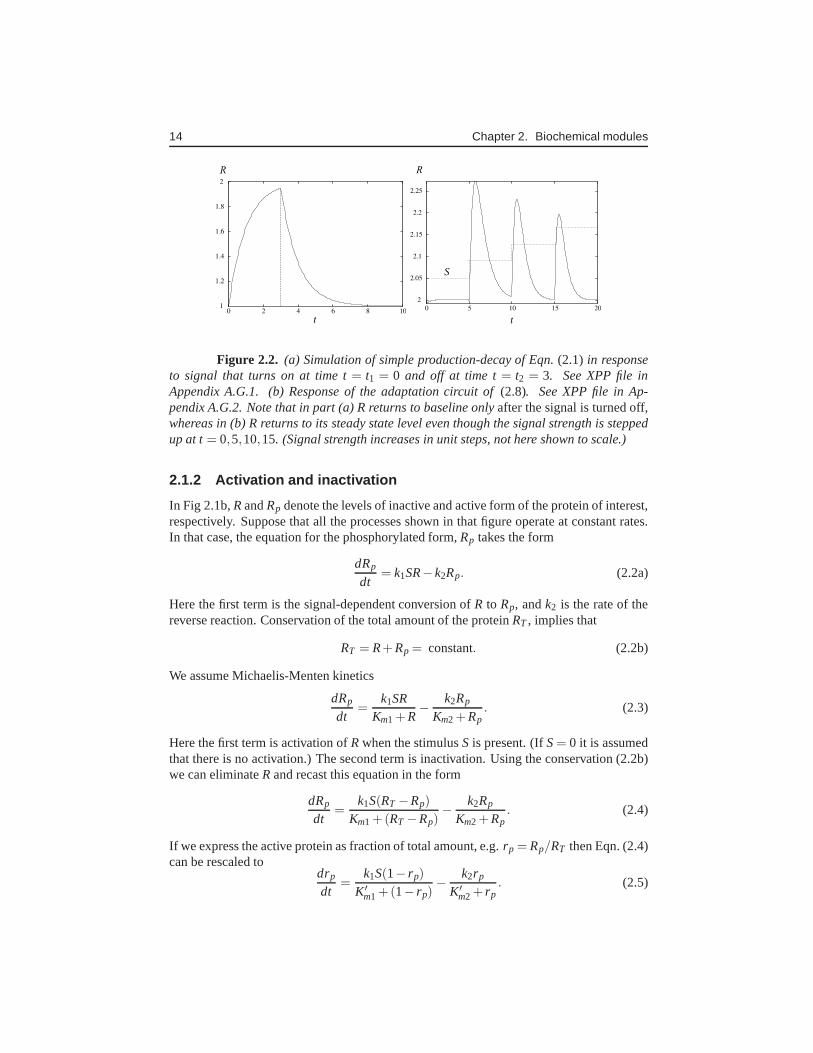
Figure 2.2. (a) Simulation of simple production-decay of Eqn.(2.1) in responseto signal that turns on at time t= t1 = 0 and off at time t= t2 = 3. See XPP file inAppendix A.G.1. (b) Response of the adaptation circuit of(2.8). See XPP file in Ap-pendix A.G.2. Note that in part (a) R returns to baseline onlyafter the signal is turned off,whereas in (b) R returns to its steady state level even thoughthe signal strength is steppedup at t= 0,5,10,15. (Signal strength increases in unit steps, not here shown toscale.)
2.1.2 Activation and inactivation
In Fig 2.1b,RandRp denote the levels of inactive and active form of the protein of interest,respectively. Suppose that all the processes shown in that figure operate at constant rates.In that case, the equation for the phosphorylated form,Rp takes the form
dRp
dt= k1SR− k2Rp. (2.2a)
Here the first term is the signal-dependent conversion ofR to Rp, andk2 is the rate of thereverse reaction. Conservation of the total amount of the proteinRT , implies that
RT = R+Rp = constant. (2.2b)
We assume Michaelis-Menten kinetics
dRp
dt=
k1SRKm1+R
− k2Rp
Km2+Rp. (2.3)
Here the first term is activation ofRwhen the stimulusS is present. (IfS= 0 it is assumedthat there is no activation.) The second term is inactivation. Using the conservation (2.2b)we can eliminateRand recast this equation in the form
dRp
dt=
k1S(RT −Rp)
Km1+(RT −Rp)− k2Rp
Km2+Rp. (2.4)
If we express the active protein as fraction of total amount,e.g.rp = Rp/RT then Eqn. (2.4)can be rescaled to
drp
dt=
k1S(1− rp)
K′m1+(1− rp)− k2rp
K′m2+ rp. (2.5)

2.1. Simple biochemical circuits with useful functions 15
0 1rp
activation inactivation
(a)
rp0 1
dr /dtp
(b)
Figure 2.3. (a) A plot of each of the two terms in Eqn.(2.5) as a function of rpassuming constant signal S. Note that one curve increases from (0,0) whereas the othercurve decreases to(1,0), and hence there is only one intersection in the interval0≤ rp≤ 1.(b) The difference of the two curves in (a). This is a plot of drp/dt and allows us to concludethat the single steady state in0≤ rp≤ 1 is stable.
Steady state(s) of (2.5) satisfy a quadratic equation. Thissuggests that there could be twosteady states, but as it turns out, only one of these need concern us, as the argument belowdemonstrates.
How does the steady state value of the response depend on the magnitude of thesignal? letu= k1S,v= k2,J = Km1,K = Km2. Note that the quantityu is proportional tothe signalS, and we will be interested in the steady state response as a function ofu. Thensolving for the steady state of (2.5) reduces to solving an equation of the form
u(1− x)J+1− x
=vx
K+ x, wherex≡ rp. (2.6)
In the exercises, we ask the reader to show that this equationreduces to a quadratic
ax2+bx+ c= 0, where a= (v−u), b= u(1−K)− v(1+ J), c= uK. (2.7)
We can write the dependence of the scaled response,rp = x on scaled signal,u. The resultis functionrp(u) that Tyson denotes the “Goldbeter-Koshland function”. (Asthis functionis slightly messy, we relegate the details of its form to Exercise 2.3.) We can plot therelationship to observe how response depends on signal. To consider a case where theenzymes operate close to saturation, let us takeK = 0.01,J= 0.02. We letv= 1 arbitrarilyand plot the responserp as a function of the “signal”u. We obtain the shape shown inFig 2.4. The response is minimal for low signal level, until some threshold aroundu≈ 1.There is then a steep rise, whenu is above that threshold, to full responserp ≈ 1. Thechange from no response to full response takes place over a very small increment in signalstrength, i.e. in the range 0.8≤ u≤ 1.2 in Fig. 2.4. This is the essence of a “zero orderultrasensitivity” switch. More details for further study of topic are given in Section??.

16 Chapter 2. Biochemical modules
u3210
1
0
rp
Res
ponse
Signal
Figure 2.4. Goldbeter Koshland “zero order ultrasensitivity”. Here u representsa stimulus (u= k1S) and rp is the response, given by a (positive) root of the quadraticequation(2.7). As the figure shows, the response is very low until some threshold level ofsignal is present. Thereafter the response is nearly 100% on. Near the threshold (aroundu= 1) it takes a very small increase of signal to have a sharp increase in the response.
2.1.3 Adaptation
Cells of the social amoebaeDictyostelium discoideumcan sense abrupt increases in theirchemoattractant (cAMP) over a wide range of absolute concentrations. In order to sensechanges, the cells exhibit a transient response, and then graduallyadapt if the cAMP levelno longer changes.
A circuit shown in Fig. 2.1c consists of an additional chemical, denoted byX that isalso made in response to signal at some constant rate. However, X is assumed to have aninhibitory effect onR, i.e. to enhance its turnover rate. The simplest form of sucha modelwould be
dRdt
= k1S− k2XR, (2.8a)
dXdt
= k3S− k4X. (2.8b)
Behaviour of (2.8) is shown in response to a changing signal in Fig. 2.2(b). After eachstep up, the system (2.8) reacts with a sharp peak of response, but that peak rapidly decaysback to baseline. Adaptation circuits of a similar type havebeen proposed by Levchenkoand Iglesias [8, 5] in extended spatial models of gradient sensing and adaptation inDic-tyostelium discoideum. In that context, they are known aslocal excitation global inhibi-tion (LEGI) models. Such work has engendered a collection of experimental approachesaimed at understanding how cells detect and respond to chemical gradients, while adaptingto uniform elevation of the chemical concentration.

2.2. Genetic switches 17
2.2 Genetic switches
A simple switch genetic switch was devised by the group of James Collins [3] using anartificially constructed pair of mutually inhibitory genes(transfected via plasmids into thebacteriumE. coli). Here each of the gene products acts as a repressor of the second gene.We examine this little genetic circuit here.
0 4
1
2
0
x
0.5
Ix
1
25
u
v
Gene U
Gene V
Figure 2.5. Right: The construction of a genetic toggle switch by Gardner et al[3], who used bacterial plasmids to engineer this circuit ina living cell. Here the twogenes, U,V produce products u,v, respectively, each of which inhibit the opposite gene’sactivity. (Black areas represent the promotor region of thegenes.) Left: a few examples ofthe functions(2.10)used for mutual repression for n= 1,2,5 in the model(2.11). Note thatthese curves become more like an on-off switch for high values of the power n.
Let us denote byu the product of one gene (U), andv the product of geneV. Eachproduct is a protein with some (relatively fixed) lifetime, i.e. degradation at constant ratecauses removal of each protein. Suppose for a moment that both genes are turned on andnot coupled to one another. In that case, we would expect their product to satisfy the pairof equations
dudt
= Iu−duu, (2.9a)
dvdt
= Iv−dvv. (2.9b)
HereIu, Iv are rates of production that depend on gene activity for genesU,V respectively,anddu,dv are the decay rates.
Now let us recraft the above to include the repression of eachproduct on the other’sgene activity. We can do so by an assumption that production of a given product decreases

18 Chapter 2. Biochemical modules
0
0.5
1
1.5
2
2.5
3
3.5
4
0 0.5 1 1.5 2 2.5 3 3.5 4
v
u
Figure 2.6. Phase plane behaviour of the toggle switch model by Gardner et al[3], given by Eqs.(2.11)with α1 = α2 = 3,n= m= 3. See XPP file in Appendix A.G.3. Thetwo steady states close to the u or v axes are stable. The one inthe center is unstable. Thenullclines are shown as the dark solid curve (u nullcline) and the dotted curve (v nullcline).
due to the presence of the other product. Gardner et al [3] assumed terms of the form
Ix =α
1+ xn . (2.10)
We plot a few curves of type (2.10) forα = 1 and various values of the powern. Thisfamily of curves intersect at the point(0,1). Forn= 1 the curve decreases gradually asxincreases. For larger powers (e.g.n= 2,n= 5), the curve has a little “shoulder”, a steepportion, and a much flatter tail, resembling the letter “Z”.
Gardner et al [3] employed the following equations (whereindu,dv were arbitrarilytaken as unit rates.)
dudt
=α1
1+ vn −u, (2.11a)
dvdt
=α2
1+um− v. (2.11b)
The behaviour of this system is shown in the phase plane of Fig. 2.6. The presence of twostable steady states is a hallmark ofbistability,.

2.3. Dimerization in a genetic switch: the λ virus 19
OR2 OR3
Repressor gene
repressor
dimer
synthesis
Figure 2.7. The phageλ gene encodes for a protein that acts as the gene’s repres-sor. The synthesized protein dimerizes and the dimers bind to regulatory sites (OR2 andOR3) on the gene. Binding to OR2 activates transcription, whereas biding to OR3 inhibitstranscription.
2.3 Dimerization in a genetic switch: the λ virus
Dimerization is a source of cooperativity that frequently appears as a motif in regulation ofgene transcription1. Here we illustrate this idea with the elegant model of Hastyet al [4]for the regulation of a gene and its product in theλ virus.
The protein of interest is transcribed from a gene known as cI(schematic in Fig. 2.7)that has a number of regulatory regions. Hasty et al considera mutant with just two suchregions, labeled OR2 and OR3. The protein synthesized from this gene transcription dimer-izes, and the dimer acts as a regulator, i.e.transcription factor for the gene. Binding ofdimer to the OR2 region of DNA activates gene transcription,whereas biding to OR3 stopstranscription.
We follow the notation in [4], definingX as the repressor,X2 a dimerized repressorcomplex,D the DNA promotor site. The fast reactions are the dimerization and binding ofrepressor to the promotor sites OR2 and OR3, for which the chemical equations are takenas
Dimerization: 2XK1−→←− X2
Binding to DNA (OR2): D+X2K2−→←− DX2
Binding to DNA (OR3): D+X2K3−→←− DX∗2
Double binding (OR2 and OR3):DX2+X2K4−→←− DX2X2 (2.12a)
Here the complexesDX2,DX∗2 are, respectively, the dimerized repressor bound to site OR2or to OR3, andDX2X2 is the state where both OR2 and OR3 are bound by dimers.
On a slower timescale, the DNA is transcribed to producencopies of the gene product
1I wish to acknowledge Alex van Oudenaarden, MIT, whose online lecture notes alerted me to this very topicalexample of dimerization and genetic switches.

20 Chapter 2. Biochemical modules
100
10
x
(a)
100
10
x
(b)
Figure 2.8. (a) A plot of the two functions given by Eqs.(2.16)for the simplifieddimensionless repressor model(2.15). (lowest dashed line:)γ = 12, (solid line:) γ = 14,and (highest dashed line:)γ = 18. (b) For γ = 14, we show the configuration of the twocurves and the positions of the resultant three steady states. The outer two are stableand the intermediate one is unstable. Compare this figure with Fig. 1.6 where a similarargument was used to understand the bifurcation structure of a simpler model involving astraight line and a Hill function.
and the repressor is degraded. The chemical equations for these are taken to be
Protein synthesis: DX2+Pk1−→ DX2+P+nX
Protein degradation:Xkd−→ A (2.12b)
We define variables as follows:x,y are the concentrations ofX,X2, respectively, andd,u,vare the concentrations ofD,DX2,DX∗2 . Similarly, z is the variable forDX2X2. The fullset of kinetic equations for this system are the topic of Exercise 2.8. However,u,v,y,z arevariables that change on a fast timescale, and a QSS approximation is applied to these.Because the total amount of DNA is constant, there is a conservation equation,
dtotal = d+u+ v+ z. (2.13)
We ask the reader [Exercise 2.8] to show that, based on the QSSapproximation for the fastvariables, the equation forx simplifies to the form
dxdt
=AK1K2x2
1+(1+σ1)K1K2x2+σ2K21K2
2x4− kdx+ r, (2.14)
whereA is a constant. This can be rewritten in dimensionless form byrescaling time andxappropriately to arrive at
dxdt
=αx2
1+(1+σ1)x2+σ2x4 − γx+1. (2.15)
2.3. Dimerization in a genetic switch: the λ virus 21
0
0.2
0.4
0.6
0.8
1
0 0.2 0.4 0.6 0.8 1
x
t
(a)
0
0.2
0.4
0.6
0.8
1
10 12 14 16 18 20
x
γ
(b)
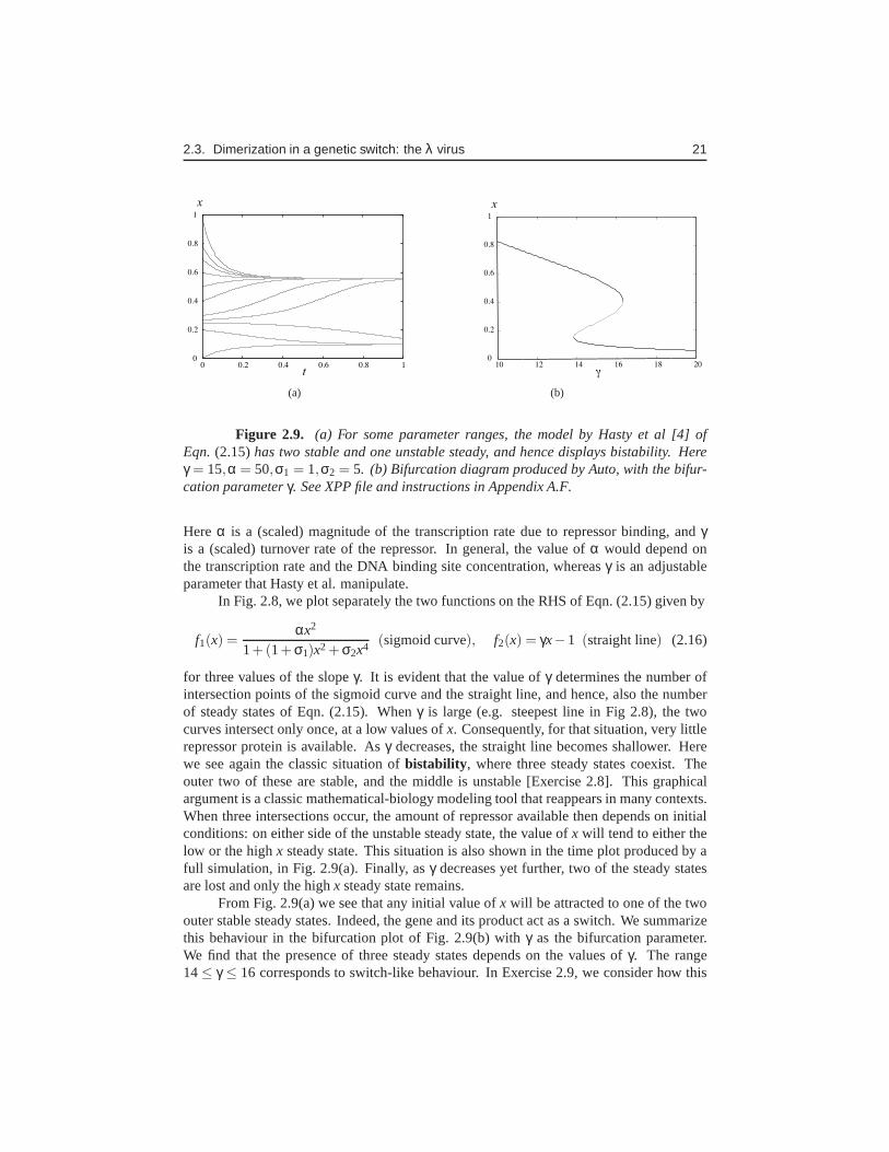
Figure 2.9. (a) For some parameter ranges, the model by Hasty et al [4] ofEqn. (2.15)has two stable and one unstable steady, and hence displays bistability. Hereγ = 15,α = 50,σ1 = 1,σ2 = 5. (b) Bifurcation diagram produced by Auto, with the bifur-cation parameterγ. See XPP file and instructions in Appendix A.F.
Hereα is a (scaled) magnitude of the transcription rate due to repressor binding, andγis a (scaled) turnover rate of the repressor. In general, thevalue ofα would depend onthe transcription rate and the DNA binding site concentration, whereasγ is an adjustableparameter that Hasty et al. manipulate.
In Fig. 2.8, we plot separately the two functions on the RHS ofEqn. (2.15) given by
f1(x) =αx2
1+(1+σ1)x2+σ2x4 (sigmoid curve), f2(x) = γx−1 (straight line) (2.16)
for three values of the slopeγ. It is evident that the value ofγ determines the number ofintersection points of the sigmoid curve and the straight line, and hence, also the numberof steady states of Eqn. (2.15). Whenγ is large (e.g. steepest line in Fig 2.8), the twocurves intersect only once, at a low values ofx. Consequently, for that situation, very littlerepressor protein is available. Asγ decreases, the straight line becomes shallower. Herewe see again the classic situation ofbistability, where three steady states coexist. Theouter two of these are stable, and the middle is unstable [Exercise 2.8]. This graphicalargument is a classic mathematical-biology modeling tool that reappears in many contexts.When three intersections occur, the amount of repressor available then depends on initialconditions: on either side of the unstable steady state, thevalue ofx will tend to either thelow or the highx steady state. This situation is also shown in the time plot produced by afull simulation, in Fig. 2.9(a). Finally, asγ decreases yet further, two of the steady statesare lost and only the highx steady state remains.
From Fig. 2.9(a) we see that any initial value ofx will be attracted to one of the twoouter stable steady states. Indeed, the gene and its productact as a switch. We summarizethis behaviour in the bifurcation plot of Fig. 2.9(b) withγ as the bifurcation parameter.We find that the presence of three steady states depends on thevalues ofγ. The range14≤ γ ≤ 16 corresponds to switch-like behaviour. In Exercise 2.9, we consider how this

22 Chapter 2. Biochemical modules
and other experimental manipulations of theλ repressor system might affect the observedbehaviour, using similar reasoning and graphical ideas.
2.4 Models for the cell division cycle
SOme of the original literature includes [12, 20, 21]. Here we mostly discuss the theoreticalpaper by Tyson and Novak [19].
G1
S-G2-M
START
FINISH
High cyclin
High APC
Figure 2.10. The cell cycle and its check points (rectangles) in the simplified modeldiscussed herein. The cycle proceeds clockwise from START.A high activity level of cyclin promotesthe START and its antagonist, APC, promotes the FINISH part of the cycle.
Cell division is conventionally divided into several phases. After a cell has divided,each daughter cell may remain for a period in a quiescent (non-growing)gap phase calledG0. Another, active (growing), gap phaseG1 precedes theS (synthesis) phase of DNAreplication. TheG2 phase intervenes betweenS phase andM phase (mitosis). During Mphase the cell material is divided. Here we will be concernedwith two checkpoints of thecycle, after G1, signaling START cell division and after S-G2-M signalling FINISH thecycle (see Fig. 2.10.) Importantly, the START checkpoint depends on the size of the cell.This requirement is essential for a balance between growth and cell division, so that cellsdo not become gigantic, nor do they produce progeny that are too tiny. (In fact mutationsthat produce one or the other form have been used by Tysonet al. as checks for validatingor rejecting candidate models.)
Control of the cell cycle is especially tight at thecheckpoints mentioned above. Forexample, the division process seems to halt temporarily at theG1 checkpoint to ascertainwhether the cell is large enough to continue to progress through the cycle or whether aprocess other than mitosis is called for (e.g., terminal cell differentiation or the alternative“meiotic” path to cell division). Once this checkpoint is passed, the cell has irreversiblycommitted to undergoing division and the process must go on.
Regulation of the cell cycle resides in a network of molecular signaling proteins. Atthe center of such a network are kinases whose activity is controlled by cyclin To sum-marize, in phase G1 there is low Cdk and low cyclin levels (cyclin is rapidly degraded).START leads to induction of cyclin synthesis and buildup of cyclin and active Cdks that

2.5. Hysteresis and bistability in cyclin and its antagonist 23
persist during the S-G2-M phases. The DNA replicates in preparation for two daughtercells. At FINISH, APC is activated, leading to destruction of cyclin and loss of CdK ac-tivity. Then the daughter cells grows until reaching a critical size where the cycle repeatsonce more.
2.4.1 Modeling conventions
Before describing the simplest model for the cell cycle, letus collect a few definitionsand conventions that will be used to construct the model. A number of these have beendiscussed previously, and we gather them here to prepare forassembling the more elaboratemodel.
Let C denote the concentration of a hypothetical protein participating in one of thereactions, and suppose thatQ is the concentration of a regulatory substance that binds toCand leads to its degradation. Then the standard way to model the kinetics ofC is
dCdt
= ksyn(substrate)− kdecayC− kassocCQ. (2.17)
Hereksyn represents a rate of protein synthesis ofC from amino acids,kassoc is rate ofassociation ofC with Q, andkdegrd is a (basal) rate of decay ofC.
Now suppose that some substance is simply converted from inactive to active formand back. Recall our discussion of activation-inactivation in Section 2.1.2. We considerthe same ideas in the case of phosphorylation and dephosphorylation under the influence ofkinases and phosphatases. We can apply the reasoning used for Eqn. (2.5) to write downour first equation. Moreover, scaling the concentration ofC in terms of the total amountCT
[Exercise 2.3c] leads to
dCdt
=K1Eactiv(1−C)
J1+(1−C)− K2EdeactivC
J2+C. (2.18)
HereJ1,J2 are saturation constants,K1,K2 are the maximal rates of each of the two reac-tions andEi are the levels of the enzymes that catalyze the activation/inactivation. Suchequations and expressions appear in numerous places in the models constructed by theTyson group for the cell division cycle.
2.5 Hysteresis and bistability in cyclin and its antagonistAn important theme in the regulatory network for cell division is that cyclin and APCare mutually antagonistic. As shown in Fig 2.11, each leads to the destruction (or lossof activity) of the other. To study this central module, Novak and Tyson considered theinteractions of just this pair of molecules. This simplifying step ignores a vast amount ofspecific detail for clarity of purpose, but leads to insightsin a modular approach promisedabove.
Let us use the following notation: LetY (cYclin) denote the level of active Cyclin-Cdk dimers, andP,Pi the levels of active (respectively inactive) APC complex. It is assumedthat the total amount of APC is constant, and scaled to 1, i.e.thatP+Pi = 1. Then based on

24 Chapter 2. Biochemical modules
Fig. 2.11 and the background of Section 2.4.1, the simplest model consists of the equations
cyclin:dYdt
= k1− (k2p+ k2ppP)Y, (2.19a)
APC:dPdt
=ViPi
J3+Pi− VaP
J4+P. (2.19b)
cyclin
A active APCinactive APC
PPi
Y
Figure 2.11. The simplest model for cell division on which Eqs.(2.21)are based.Cyclin (Y) and APC (P) are mutually antagonistic. APC leads to the degradation of cyclin,and cyclin deactivates APC.
The rates of the reactions are not constant. That is because aprotein called hereA,(and for now held fixed) is assumed to enhance the forward reaction, activating APC andcyclin (Y) enhances the reverse reaction, deactivating it. Tyson andNovak assume that:
Vi = (k3p+ k3ppA), Va = k4mY.
Here,m denotes the mass of the cell, a quantity destined to play an important role in themodel(s) to be discussed2. Recall that cell mass (for now considered fixed) is known toinfluence the decision to pass the START checkpoint. Thus, the model becomes
dYdt
= k1− (k2p+ k2ppP)Y, (2.20a)
dPdt
=(k3p+ k3ppA)Pi
J3+Pi− k4m
YPJ4+P
. (2.20b)
By conservation of the total amount of APC, and the scaling wehave used,
Pi = 1−P.
2The reader will note that cell massm is introduced already in the simplest model as a parameter, and thatas the models become more detailed, the role of this quantitybecomes more important. In the final models wediscuss,m is itself a variable that changes over the cycle and influences other variables. L.E.K.

2.5. Hysteresis and bistability in cyclin and its antagonist 25
Hence,
dYdt
= k1− (k2p+ k2ppP)Y, (2.21a)
dPdt
=(k3p+ k3ppA)(1−P)
J3+(1−P)− k4m
YPJ4+P
. (2.21b)
This constitutes the first minimal model for cell cycle components, and our first task willbe to explore the bistability in this system.
0
0.2
0.4
0.6
0.8
1
P
0 0.2 0.4 0.6 0.8 1Y
P nullcline
Y nullcline
Low m
(a)
0
0.2
0.4
0.6
0.8
1
0 0.2 0.4 0.6 0.8 1
P nullcline
Y nullcline
Y
P
High m
(b)
Figure 2.12. The YP phase plane for Eqs.(2.21)and parameter values as shownin the XPP file in Appendix A.H.1. Parameters with units of 1/time are: k1 = 0.04,k2p =0.04,k2pp = 1,k3p = 1,k3pp = 10,k4 = 35, Other (dimensionless) parameters are: A=0,J3 = 0.04,J4 = 0.04. Here the cell mass is as follows: (a) m= 0.3. There are threesteady states, a stable node at low Y high P (0.038, 0.96), a stable node at high Y low P(0.9,0.0045), and a saddle point at intermediate levels of both (0.1, 0.36). (b) m= 0.6.The nullclines have moved apart so that there is a single (stable) steady state at(Y,P) =(0.9519,0.002): this state has high level of cyclin, and very little APC.
Figure 2.12 shows the typical phase-plane portrait of Eqs. (2.21), with theY andPnullclines in dashed and solid lines, respectively. There are three steady states identifiedwith the checkpoints at G1 and at S-G2-M. As the cell grows, its massm increases. Asshown in Fig. 2.12(a), this pushes theP nullcline to the left so that eventually, two pointsof intersection with they nullcline disappear. (Just as this occurs, the saddle pointand G1steady state merge and vanish. This explains the termsaddle-node bifurcation appliedto such a transition, also called afold bifurcation.) Parameter values of this model areprovided in [19] and in the XPP file in Appendix A.H.1. We find that, at the bifurcation,transition to S-G2-M is very rapid once the GI checkpoint hasbeen lost.
We show the bifurcation diagram for Eqs. (2.21) in Fig. 2.13(a), with cell massm asthe bifurcation parameter,. Then in Fig. 2.13(b), we identify steady states and the transi-tion between them with parts of the cell cycle. We see the property of hysteresis that ischaracteristic of bistable systems: the parameterm has to increase to a high value to trig-ger the START transition, and then cell mass has to decrease greatly to signal the FINISHtransition. Here the latter is associated with cell division at whichm drops by a factor of 2.
26 Chapter 2. Biochemical modules
0
0.4
0.8
1.2
Y
0 0.2 0.4 0.6
m
(a)
0
0.4
0.8
1.2
Y
0 0.2 0.4 0.6
m
START
FINISH
S-G2-M
G1
(b)
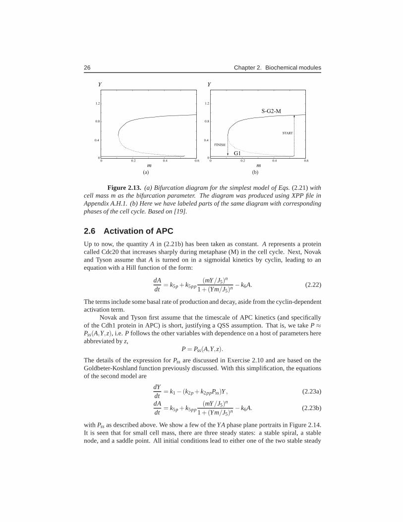
Figure 2.13. (a) Bifurcation diagram for the simplest model of Eqs.(2.21)withcell mass m as the bifurcation parameter. The diagram was produced using XPP file inAppendix A.H.1. (b) Here we have labeled parts of the same diagram with correspondingphases of the cell cycle. Based on [19].
2.6 Activation of APCUp to now, the quantityA in (2.21b) has been taken as constant.A represents a proteincalled Cdc20 that increases sharply during metaphase (M) inthe cell cycle. Next, Novakand Tyson assume thatA is turned on in a sigmoidal kinetics by cyclin, leading to anequation with a Hill function of the form:
dAdt
= k5p+ k5pp(mY/J5)
n
1+(Ym/J5)n − k6A. (2.22)
The terms include some basal rate of production and decay, aside from the cyclin-dependentactivation term.
Novak and Tyson first assume that the timescale of APC kinetics (and specificallyof the Cdh1 protein in APC) is short, justifying a QSS assumption. That is, we takeP≈Pss(A,Y,z), i.e. P follows the other variables with dependence on a host of parameters hereabbreviated byz,
P= Pss(A,Y,z).
The details of the expression forPss are discussed in Exercise 2.10 and are based on theGoldbeter-Koshland function previously discussed. With this simplification, the equationsof the second model are
dYdt
= k1− (k2p+ k2ppPss)Y, (2.23a)
dAdt
= k5p+ k5pp(mY/J5)
n
1+(Ym/J5)n − k6A. (2.23b)
with Pssas described above. We show a few of theYAphase plane portraits in Figure 2.14.It is seen that for small cell mass, there are three steady states: a stable spiral, a stablenode, and a saddle point. All initial conditions lead to either one of the two stable steady
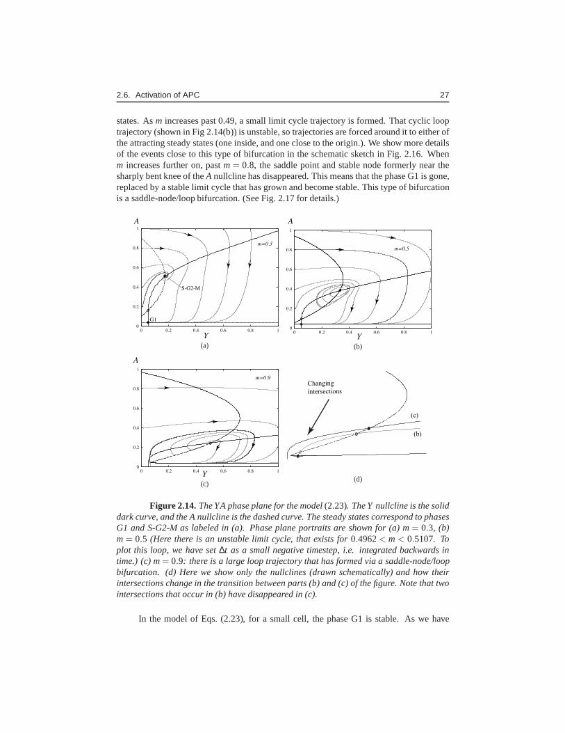
2.6. Activation of APC 27
states. Asm increases past 0.49, a small limit cycle trajectory is formed. That cyclic looptrajectory (shown in Fig 2.14(b)) is unstable, so trajectories are forced around it to either ofthe attracting steady states (one inside, and one close to the origin.). We show more detailsof the events close to this type of bifurcation in the schematic sketch in Fig. 2.16. Whenm increases further on, pastm= 0.8, the saddle point and stable node formerly near thesharply bent knee of theA nullcline has disappeared. This means that the phase G1 is gone,replaced by a stable limit cycle that has grown and become stable. This type of bifurcationis a saddle-node/loop bifurcation. (See Fig. 2.17 for details.)
0
0.2
0.4
0.6
0.8
1
0 0.2 0.4 0.6 0.8 1
m=0.3
Y
A
G1
S-G2-M
(a)
0
0.2
0.4
0.6
0.8
1
0 0.2 0.4 0.6 0.8 1
Y
A
m=0.5
(b)
0
0.2
0.4
0.6
0.8
1
0 0.2 0.4 0.6 0.8 1Y
A
m=0.9
(c)
Changing
intersections
(b)
(c)
(d)
Figure 2.14. The YA phase plane for the model(2.23). The Y nullcline is the soliddark curve, and the A nullcline is the dashed curve. The steady states correspond to phasesG1 and S-G2-M as labeled in (a). Phase plane portraits are shown for (a) m= 0.3, (b)m= 0.5 (Here there is an unstable limit cycle, that exists for0.4962< m< 0.5107. Toplot this loop, we have set∆t as a small negative timestep, i.e. integrated backwards intime.) (c) m= 0.9: there is a large loop trajectory that has formed via a saddle-node/loopbifurcation. (d) Here we show only the nullclines (drawn schematically) and how theirintersections change in the transition between parts (b) and (c) of the figure. Note that twointersections that occur in (b) have disappeared in (c).
In the model of Eqs. (2.23), for a small cell, the phase G1 is stable. As we have

28 Chapter 2. Biochemical modules
seen above, the growth of that mass eventually leads to “excitable” dynamics, where asmall displacement from G1 results in a large excursion (Fig2.14(b)) before returningto G1. When the mass is even larger, G1 disappears altogetherand a cyclic behaviourensues. However, this is linked to division of the cell mass so thatm falls back to low level,reestablishing the original nullcline configuration and returning to the beginning of the cellcycle.
2.6.1 The three-variable YPAmodel
We are now interested in exploring the three-variable modelwithout the QSS assumptiononP. Consequently, we adopt the set of three dynamic equations
dYdt
= k1− (k2p+ k2ppP)Y, (2.24a)
dPdt
=(k3p+ k3ppA)(1−P)
J3+(1−P)− k4m
YPJ4+P
, (2.24b)
dAdt
= k5p+ k5pp(mY/J5)
n
1+(Ym/J5)n − k6A. (2.24c)
with the same decay and activation functions as before. We keep m, all k’s and J’s asconstants at this point. The model is more intricate than that of (2.21), and the bifurcation
0.1
0.2
0.3
0.4
0.5
0.2 0.4 0.6 0.8 1
Y
m
SbH
SNL
SN
(Limit cycle)
(a)
0.1
0.2
0.3
0.4
0.5
0.2 0.4 0.6 0.8 1
Y
m
G1
S-G2-M
start
finish
(b)
Figure 2.15. (a) Bifurcation diagram for the full YPA model given by Eqs.(2.24)produced by the XPP file and instructions in the Appendix A.H.3. Bifurcations labeled onthe diagram include a fold (saddle node, SN) bifurcation, a subcritical Hopf (SbH) and asaddle-node loop (SNL) bifurcation. The open circles represent an unstable limit cycle, asseen in Fig 2.14(b) of the QSS version of the model. The filled circles represent the stablelimit cycle analogous to the one seen in Fig 2.14(c). (b) The course of one cell cycle issuperimposed on the bifurcation diagram. The cell starts atthe low cyclin state (G1) alongthe lower branch of the bistable curve. As cell mass increases, the state drifts towards theright along this branch until the SNL bifurcation. At this point a stable limit cycle emerges.This represents the S-G2-M phase, but as the cell divides, its mass is reset back to a smallvalue of m, setting it back to G1.
2.6. Activation of APC 29
plot hence trickier to produce (but see instructions in Appendix A.H.3). However, withsome persistence this is accomplished, yielding Figure 2.153.
Let us interpret Figure 2.15. In panel 2.15(a), we show the cyclin levels against cellmassm, the bifurcation parameter. (Cell mass increases along thelower axis to the right, asbefore.) Labeled on the diagram in 2.15(a) are several bifurcations (see caption), the mostimportant being the saddle-node/loop bifurcation (SNL). Once cell mass grows beyondthis critical value ofm≈ 0.8, the lower G1 steady state disappears, and is replaced by astable limit cycle. This is precisely the kind of transitionwe have already seen in Fig 2.14(between the configurations in 2.14(b) and 2.14(c)).
Figure 2.15(b), we repeat the bifurcation diagram, but thistime we superimpose atypical “trajectory” over one whole cell division cycle: the system starts in the lower rightpart of the diagram at G1, progresses to higher cell mass, passes the START checkpoint,duplicates DNA in the S-G2-M phase and then divides into two progeny, each of whosemass is roughly 1/2 of the original mass. This meansmdrops back to its low value for eachprogeny, and daughter cells are thereby back at G1.
a < acrit a > acrit a >> acrit
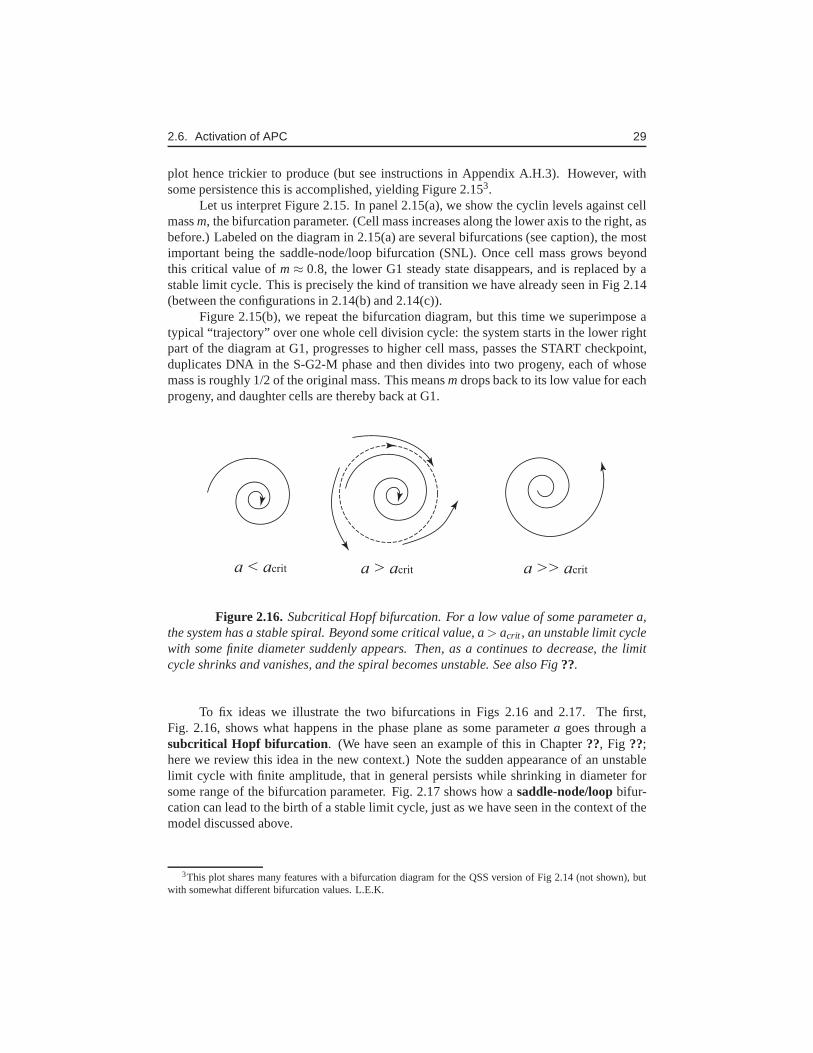
Figure 2.16. Subcritical Hopf bifurcation. For a low value of some parameter a,the system has a stable spiral. Beyond some critical value, a> acrit , an unstable limit cyclewith some finite diameter suddenly appears. Then, as a continues to decrease, the limitcycle shrinks and vanishes, and the spiral becomes unstable. See also Fig??.
To fix ideas we illustrate the two bifurcations in Figs 2.16 and 2.17. The first,Fig. 2.16, shows what happens in the phase plane as some parametera goes through asubcritical Hopf bifurcation. (We have seen an example of this in Chapter??, Fig ??;here we review this idea in the new context.) Note the sudden appearance of an unstablelimit cycle with finite amplitude, that in general persists while shrinking in diameter forsome range of the bifurcation parameter. Fig. 2.17 shows howa saddle-node/loop bifur-cation can lead to the birth of a stable limit cycle, just as wehave seen in the context of themodel discussed above.
3This plot shares many features with a bifurcation diagram for the QSS version of Fig 2.14 (not shown), butwith somewhat different bifurcation values. L.E.K.

30 Chapter 2. Biochemical modules
a < acrit a = acrit a > acrit
Figure 2.17. Saddle-node/loop bifurcation here involves an unstable spiral and asaddle point. As some bifurcation parameter, a, changes, the transitions shown here takeplace. When a= acrit , there is a heteroclinic trajectory that connects the saddle point toitself. For larger values of a, a limit cycle appears and the heteroclinic loop disappears.At first appearance, the period of the limit cycle is very long(“infinitely long”) due to thevery slow motion along the portion of the trajectory close tothe saddle point.
2.6.2 A fuller basic model
The models considered so far have included only the skeletalforms of the regulatory celldivision components. Including some additional interactions [19, p 255] results in a slightlyexpanded version suitable for describing the cell cycle of budding yeast. The notationfor this model is provided in Table 2.1 and interactions between these are illustrated inFigure 2.18.
The equations are given by the following:
cyclin:dYdt
= k1− (k2p+ k2ppP)Y, (2.25a)
APC:dPdt
=(k3p+ k3ppAA)(1−P)
J3+(1−P)− k4m
YPJ4+P
, (2.25b)
Total A:dAT
dt= k5p+ k5pp
(mY/J5)n
1+(Ym/J5)n − k6AT , (2.25c)
Active A:dAA
dt= k7IP
AT −AA
J7+AT −AA− k6AA− k8[Mad]
AA
J8+AA, (2.25d)
IEP:dIPdt
= k9mY(1− IP)− k10IP, (2.25e)
cell mass:dmdt
= µm
(
1− mms
)
. (2.25f)
Eqs (2.25a) and (2.25b) for cyclin and APC have not changed since the previousmodel. As in theYPAthree-variable model, APC is activated by the substanceA (specif-ically Cdc20). However, we now distinguish between the active form, AA, and the totalamount,AT of Cdc20. This protein is assumed to be inactive when first synthesized. Thebasal synthesis rate, shown ask5p in (2.25c) is enhanced in the presence of high cyclin orwhen the cell mass is large (Hill function in the second term), as in the previous model.
2.6. Activation of APC 31
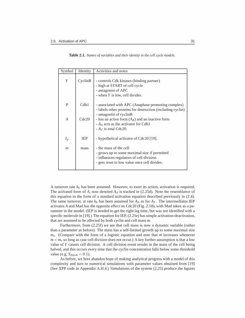
Table 2.1. Names of variables and their identity in the cell cycle models.
Symbol Identity Activities and notes
Y CyclinB - controls Cdk kinases (binding partner)- high at START of cell cycle- antagonist of APC- whenY is low, cell divides.
P Cdh1 - associated with APC (Anaphase promoting complex)- labels other proteins for destruction (including cyclin)- antagonist of cyclinB
A Cdc20 - has an active form (AA) and an inactive form- AA acts as the activator for Cdh1- AT is total Cdc20.
Ip IEP - hypothetical activator of Cdc20 [19].
m mass - the mass of the cell- grows up to some maximal size if permitted- influences regulators of cell division- gets reset to low value once cell divides.
A turnover ratek6 has been assumed. However, to exert its action, activation is required.The activated form ofA, now denotedAA is tracked in (2.25d). Note the resemblance ofthis equation to the form of a standard activation equation described previously in (2.4).The same turnover, at ratek6 has been assumed forAA as forAT . The intermediates IEPactivatesA and Mad has the opposite effect on Cdc20 (Fig. 2.18), with Madtaken as a pa-rameter in the model. (IEP is needed to get the right lag time,but was not identified with aspecific molecule in [19].) The equation for IEP, (2.25e) hassimple activation-deactivation,that are assumed to be affected by both cyclin and cell massm.
Furthermore, from (2.25f) we see that cell mass is now a dynamic variable (ratherthan a parameter as before). The mass has a self-limited growth up to some maximal sizems. (Compare with the form of a logistic equation and note thatm increases wheneverm< ms so long as case cell division does not occur.) A key further assumption is that a lowvalue ofY causes cell division. A cell division event results in the mass of the cell beinghalved, and this occurs every time that the cyclin concentration falls below some thresholdvalue (e.g.Ythresh= 0.1).
As before, we here abandon hope of making analytical progress with a model of thiscomplexity and turn to numerical simulations with parameter values obtained from [19](See XPP code in Appendix A.H.4.) Simulations of the system (2.25) produce the figures

32 Chapter 2. Biochemical modules
G1
S-G2-M
START
FINISH
IE IEP
AT
cYclin
AA
Mad
aPc
Figure 2.18. The full model of the cell cycle depicted in Eqs.(2.25). At its core isthe simpler YPA module, but other regulatory parts of the network have been added. SeeTable 2.1 for definitions of all components.
shown in Fig 2.19. We note the following behaviour: At the core of the mechanism thereis still the same antagonism between cyclin and APC: Now bothvary periodically over thecell cycle, but they do so out of phase: APC is high when cyclinis low and vice versa. Thetotal and active Cdc20, as well as the IEP shown in the third panel. Careful observationdemonstrates thatAT cycles in phase cyclin, but activation takes longer, so thatAA peaksjust asY is dropping to a low level.AA andIP are in phase. Cell mass is a saw-tooth curve,with division coinciding with the sharp drop in cyclin levels.
Exercises2.1. Suppose thatS,ki > 0 for i = 0,1,2 in Eqn. (2.1).
(a) Find the solutionR(t) to this equation.
(b) Find the steady state of the same equation.

Exercises 33
0.1
0.2
0.3
0.4
0.5
0.6
0.7
0.8
0.9
0 50 100 150 200 250 300
cyclin
APC
t
0
0.2
0.4
0.6
0.8
1
0 50 100 150 200 250 300
Cell Mass
t0
0.2
1
1.8
0 50 100 150 200 250 300
Cdc20T
Cdc20A
IEP
t
Figure 2.19. Time behaviour of variables in the extended model of Eqs.(2.25).Plots produced with the XPP file in Appendix A.H.4.
(c) Show that the steady state response depends linearly on the strength of thesignal.
(d) What happens if initiallyS= 0, and then at timet = 0 S is turned on? Howcan this be recast as an initial value problem involving the same equation?
(e) Now suppose thatS is originally ON (e.g.S= 1), but then, att = 0, the signalis turned OFF. Answer the same question as in part (d).
(f) Based on your responses to (d) and (e), what would happen if the signal isturned on at some timet1 and off again at a later timet2? Sketch the (approxi-mate) behaviour ofR(t).
(g) Create a simple XPP file and compare your answers to results of simulations.
2.2. Consider the simple phosphorylation-dephosphorylationmodel given by (2.2a). Whatis the analogous differential equation forR? Find the steady state concentration forRp and show that it saturates with increasing levels of the signal S. [Hint: eliminate

34 Chapter 2. Biochemical modules
R using the fact that the total amount,R+Rp is conserved.] Assume thatk1,S,k2
are all positive constants in this problem.
2.3. (a) Redraw Fig. 2.1 with parameterski labeled on the various arrows. Explainwhat are the assumptions underlying Eqn. (2.3). Show that conservation leadsto (2.4).
(b) What would be the corresponding equation for the unphosphorylated formR?
(c) Rescale the variableRby the (constant) total amountRT in Eqn. (2.4).
(d) Solving for the steady state of the equation you got in part (c) leads to aquadratic equation. Write down that quadratic equation forRp,SS. Show thatyour result is in the form of (2.7) (Once the appropriate substitutions are made).
(e) Solve the quadratic equation, (2.7), in terms of the coefficientsa,b,c, and thenrewrite your result in terms of the parametersu,v,K,J. This (somewhat messyresult) is the so-called Goldbeter-Koshland function.
(f) According to Novak and Tyson [19], the Goldbeter-Koshland function has theform
G(u,v,J,K) =2γ
β+√
β2−4αγ.
for α,β,γ similar expressions ofu,v,J,K. How does this fit with your result?Hint: recall that the an expression with radical denominator can be rational-ized, as follows
1p+√
q=
p−√q
(p+√
q)(p−√q)=
p−√q
p2−q.
2.4. Consider the adaptation module shown in Fig. 2.1c and given by Eqs. (2.8).
(a) Show that the steady state level ofR is the same regardless of the strength ofthe signal.
(b) Is the steady state level ofX also independent of signal? Sketch the (approx-imate) behaviour ofX(t) corresponding to the result forR and S shown inFig. 2.2(b)
(c) Use the XPP file provided in Appendix A.G.2 to simulate this model with avariety of signals and initial conditions.
(d) How do the parameterski in Eqs. (2.8) affect the degree of adaptation? Whatif X changes very slowly? very quickly relative toR? (Experiment with thesimulation or consider analyzing the problem in other ways.)
2.5. Here we consider Eqs. (2.8) using phase-plane methods,and assuming thatS isconstant.
(a) Sketch theX andRnullclines in theXRplane.
(b) Show that there is only one intersection point, i.e. a unique steady state, andthat this steady state is stable.
(c) Explain how the phase plane configuration changes whenS is instantaneouslyincreased, e.g. fromS= 1 to S= 2.

Exercises 35
2.6. Consider the genetic toggle switch by Gardner et al [3],given by the model equa-tions Eqs. (2.11).
(a) Consider the situation thatn= 1 in the repression term of the function (2.10)and in the model equations. Solve for the steady state solution(s) to Eqs. (2.11).
(b) Your result in (a) would have led to solving a quadratic equation. How manysolutions are possible? How many (biologically relevant) steady states willthere be?
(c) Consider the shapes of the functionsIx shown in Fig. 2.5. Using these shapes,sketch the nullclines in the phase plane forn= m= 1 and forn,m> 1. Howdoes your sketch inform the dependence of bistability on these powers?
(d) Now suppose thatn= m= 3 (as in Fig 2.6). How do the valuesαi affect thesenullcline shapes? Supposeα1 is decreased or increased. How would this affectthe number and locations of steady state(s)?
(e Explore the behaviour of the model by simulating it using the XPP file in Ap-pendix A.G.3 or your favorite software. Show that the configuration shown inFig. 2.6 with three steady states depends on appropriate choices of the integerpowersn,m, and comment on these results in view of part (c) of this exercise.
(f) Further explore the effect of the parametersαi . How do your conclusionscorrespond to part (d) above?
2.7. Consider the genetic toggle switch in the situation shown in Fig. 2.6.
(a) Starting withu= 2, what is the minimal value ofv that will throw the switchto v (i.e., lead to the highv steady state)?
(b) Fig. 2.6 shows some trajectories that “appear” to approach the white dot in theuvplane. Why does the switch not get “stuck” in this steady state?
(c) Suppose that the experimenter can manipulate the turnover rate ofu so that it isdu = 1.5 (rather thandu = 1 and in (2.11)). How would this affect the switch?
2.8. Consider the chemical scheme proposed by Hasty et al [4]in (2.12).
(a) Write down the differential equations for the variablesx,y,u,v,d correspond-ing to these chemical equations. (To do so, first replace the capitalized rateconstants associated with the reversible reactions with forward and reverseconstants (e.g.K1 is replaces byκ1,κ−1 etc).)
(b) Hasty et al assume that Eqs. (2.12a) arefast, i.e. are at quasi-steady state. Showthat this leads to the following set of algebraic equations for these variables:
y= K1x2, (2.26a)
u= K2dy= K1K2dx2, (2.26b)
v= σ1K2dy= σ1K1K2dx2, (2.26c)
z= σ2K2uy= σ2(K1K2)2dx4. (2.26d)
(c) Show that this QSS assumption together with the conservation equation (2.13)leads to the differential equation forx given by (2.14).

36 Chapter 2. Biochemical modules
(d) Show that the equation you obtained in part (c) can be rewritten in the dimen-sionless form (2.15).
(e) Run the XPP code in Appendix A.F with the default values ofparameters, andthen changeγ to each of the following values: (i)γ= 12 (ii) γ= 14, (iii) γ= 16,(iv) γ = 18. Comment on the number and stability of steady states.
(f) Connect the behaviour you observed in part (e) with the bifurcation diagramin Fig 2.9(b).
2.9. Consider theλ repressor gene model by Hasty et al [4], and in particular themodel(2.15) discussed in the text. Suppose an experimenter carries out the following ex-perimental manipulations of the system. State how the equation would change, orwhich parameter would change, and what would be the effect onthe behaviour ofthe system. Use graphical ideas to determine the qualitative outcomes (The manip-ulations may affect some slope, height, etc. of a particularcurve in Fig. 2.8.)
(a) The experimenter continually adds repressor at some constant rate to the sys-tem.
(b) The experimenter inhibits the turnover rate of repressor protein molecules.
(c) Repeat (b), but this time, the experimenter can control the turnover rate care-fully and incrementally increases that rate from a low degradation level viaintermediate level, to high level. What might be seen as a result?
(d) The experimenter inhibits the transcription rate in thecell, so that repressormolecules are made at a lower rate when the gene is active.
2.10. In the cell cycle model of Section 2.6, it is assumed that the variableP given byEqn. (2.21b) is on quasi-steady state (QSS). Here we explorethat relationship.
(a) Assume thatdP/dt = 0 in (2.21b) and show that you arrive at a quadraticequation. Note similarity to Exercise 2.3d.
(b) Write down the solution to that quadratic equation.
(c) Show that you arrive at the Goldbeter-Koshland function, as in Exercise 2.3.
G(Va,Vi ,Ja,Ji)=2VaJi
(Vi−Va+VaJi +ViJa+√
(ViVa+VaJi +ViJa)2−4(Vi−Va)VaJi
2.11. Here we further explore the YP model of Eqs. (2.21) shown in Fig 2.12. Use theXPP file provided in Section A.H.1 (or your favorite software) to investigate thefollowing:
(a) Replot the YP phase plane and add trajectories to the two diagrams shown inFigs. 2.12(a) and 2.12(a).
(b) Use your exploration in part (a) to determine the basin ofattraction of each ofthe steady states in Figs. 2.12(a).
(c) Follow the instructions provided in Section A.H.1 to reproduce the bifurcationdiagram in Fig. 2.13.
2.12. Consider the three variableYPAmodel for the cell cycle given by Eqs. 2.24

Exercises 37
(a) Simulate the model using the XPP file provided Appendix A.H.3 (or your fa-vorite software) for values of the cell mass in the ranges of interest shownin Fig 2.15, i.e. for low, intermediate, and larger cell mass. Sketch the timebehaviour ofY,P,A for these simulations.
(b) Follow the instructions in Appendix A.H.3 to reproduce the bifurcation picturefor this model.
2.13. Consider the following set of equations:
dxdt
= αx− y− x(x2+ y2), (2.27a)
dydt
= x+αy− y(x2+ y2). (2.27b)
This set of equations represents the classic (supercritical) Hopf bifurcation, in whicha stable limit cycle appears and gradually grow in diameter at a rate
√α−αcrit .
(a) Explore this system numerically for a range of values ofα to find its stablelimit cycle.
(b) Now consider the related system that has a subcritical Hopf bifurcation
dxdt
= αx− y+ x(x2+ y2), (2.28a)
dydt
= x+αy+ y(x2+ y2). (2.28b)
Study this system using the same methods and compare your results. Youshould find that an (unstable) limit cycle appears with nonzero diameter, andshrinks as the bifurcation parameter increases.
2.14. Use the XPP file provided in Appendix A.H.4 (or your favorite software) to simulatethe model of Eqs. (2.25). Compare the time behaviour of APC and cyclin obtainedin this model (e.g. in the first panel of Fig 2.19) with the corresponding behavioursobtained in the two and the three variable models.

38 Chapter 2. Biochemical modules
includechapters/chapFEMCB

Chapter 3
Simple polymers
3.1 Simple models for polymer growth dynamics
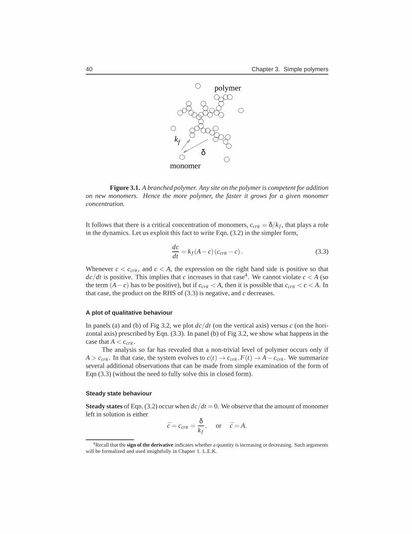
3.1.1 Simple aggregation of monomers
We first look at simple aggregation where monomers can be added anywhere on the grow-ing polymer. An example of this type could be highly branchedpolymer where every site isaccessible for further addition, as shown in Fig 3.1. An example of this type was proposedby [11] to describe the aggregation of amyloid monomers intofibrils. Let us define thefollowing variables:
c(t) = number of monomer subunits in the volume at timet,
F(t) = amount of polymer (in number of monomer equivalents) at timet,
A(t) = total amount of material (in number of monomer equivalents)at timet.
( F is given a value that corresponds to the concentration of that much liberated monomerin the same reaction volume.)
Assume: The rate of growth depends on a product ofc andF, with rate constantkf > 0 (forward reaction rate) and the rate of disassembly or turnover is linearly propor-tional to the amount of polymer, with rate constantδ. Note thatA = c+F is constant[Exercise 3.1(a)]. Our model equations are then:
dcdt
=−kf cF+ δF, (3.1a)
dFdt
= kf cF− δF. (3.1b)
EliminatingF by settingF = A− c leads to a single equation for monomers:
dcdt
= (−kf c+ δ)F = kf (A− c)
(
δkf− c
)
(3.2)
39
40 Chapter 3. Simple polymers
δ
kf
polymer
monomer
Figure 3.1. A branched polymer. Any site on the polymer is competent for additionon new monomers. Hence the more polymer, the faster it grows for a given monomerconcentration.
It follows that there is a critical concentration of monomers,ccrit = δ/kf , that plays a rolein the dynamics. Let us exploit this fact to write Eqn. (3.2) in the simpler form,
dcdt
= kf (A− c)(ccrit − c) . (3.3)
Wheneverc < ccrit , andc < A, the expression on the right hand side is positive so thatdc/dt is positive. This implies thatc increases in that case4. We cannot violatec< A (sothe term(A−c) has to be positive), but ifccrit < A, then it is possible thatccrit < c< A. Inthat case, the product on the RHS of (3.3) is negative, andc decreases.
A plot of qualitative behaviour
In panels (a) and (b) of Fig 3.2, we plotdc/dt (on the vertical axis) versusc (on the hori-zontal axis) prescribed by Eqn. (3.3). In panel (b) of Fig 3.2, we show what happens in thecase thatA< ccrit .
The analysis so far has revealed that a non-trivial level of polymer occurs only ifA> ccrit . In that case, the system evolves toc(t)→ ccrit ,F(t)→ A− ccrit . We summarizeseveral additional observations that can be made from simple examination of the form ofEqn (3.3) (without the need to fully solve this in closed form).
Steady state behaviour
Steady states of Eqn. (3.2) occur whendc/dt= 0. We observe that the amount of monomerleft in solution is either
c= ccrit =δkf
, or c= A.
4Recall that thesign of the derivative indicates whether a quantity is increasing or decreasing. Such argumentswill be formalized and used insightfully in Chapter 1. L.E.K.

3.1. Simple models for polymer growth dynamics 41
ccrit A
dc/dt
c0
dc/dt
c0 A c
crit
(a) (b)
0
0.5
1
1.5
2
2.5
3
0 2 4 6 8 10
Polymer
Monomer
0
0.2
0.4
0.6
0.8
1
0 5 10 15 20
Monomer
Polymer
(c) (d)
Figure 3.2. Polymerization kinetics in simple aggregation. State space plots of(3.3) (also called phase portraits) showing monomer (c) and polymer (F) levels for con-stant total amount (A). (a) A> ccrit = δ/kf : in this case, c, will always approach its criticalconcentration,c = ccrit = δ/kf , (b) A< ccrit : here there will be only monomers, and nopolymers will form. The grey region is an irrelevant regime,since the level of monomercannot exceed the total amount of material, A. Time plots of the two cases, produced byXPP (c) for A> ccrit , (d) for A< ccrit . Parameter values: kf = 1,δ = 1,A= 3. XPP codecan be found in Appendix A.A.
The amount of polymer at this steady state is (by conservation), F ≡ F = A− ccrit = A−δ/kf , or F = 0. Beyond the critical concentration, i.e. forc> ccrit , adding more monomerto the system (which thus increases the total amountA) will not increase the steady statelevel of monomer, only the polymerized form.
Initial rise time
The initial rate of the reaction, when the mixture just starts to grow: Suppose that initially,there is only a little bit of polymer to seed the reaction, i.e. F(0) = ε, c(0) = A− ε ≈ Afor some smallε > 0. Then a good approximation of the polymer kinetics is givenbysubstitutingc≈ A into the above equation to get
dFdt≈ kf (A− ccrit )F = KF.
42 Chapter 3. Simple polymers
whereK = kf (A−ccrit ) is a positive constant. Then the initial time behaviour of filaments,F(t) = εexp(Kt), is exponentially growing providedA> ccrit .
Decay behaviour if monomer is removed
If the monomer is “washed away” from a mature reaction, i.e. effectively settingc= 0 inEqn. (3.1b) leads to gradual disassembly of polymer, since then
dFdt≈−δF.
The polymer will decay exponentially with rate constantδ, i.e. F(t) = F0exp(−δt). Thiscan be useful in determining values of parameters from data.
The full kinetic behaviour
Having identified main qualitative features of the system, and a few special cases such asearly time behaviour, we turn to a full solution. Here we use software to numerically inte-grate the system of equations (3.1) and show the behaviour for a specific set of parametervalues. We show this behaviour in panels (c) and (d) of Fig. 3.2. There are many soft-ware packages that can easily handle such differential equations. Here we use XPP (codeprovide in Appendix A.A).
Summary and observations
It is useful to gather the results of our simple analysis. We will find that such observationswill help us later in distinguishing between one type of aggregation reaction and another.
3.1.2 Linear polymer growing at their tips
Here is a slightly different scenario, in which nucleation occurs only at some sites. Forexample, we consider a linear polymer with growth exclusively at the end(s) of the fila-ments, as shown in Fig 3.3. We keep the previous assumption that disassembly takes placeby some bulk turnover of the polymer, i.e., not necessarily by monomer loss at the ends.We guide the reader through exploration of this case in Exercise 3.3, with main conceptssummarized here more briefly.
We will define:
n= Number of filaments (or filament tips) at which polymerization can occur.
We assume at this stage that the number of filament tips,n, is constant, and that neitherbreakage nor branching takes place. Then the appropriate model is
dcdt
=−kf cn+ δF, (3.4a)
dFdt
= kf cn− δF. (3.4b)
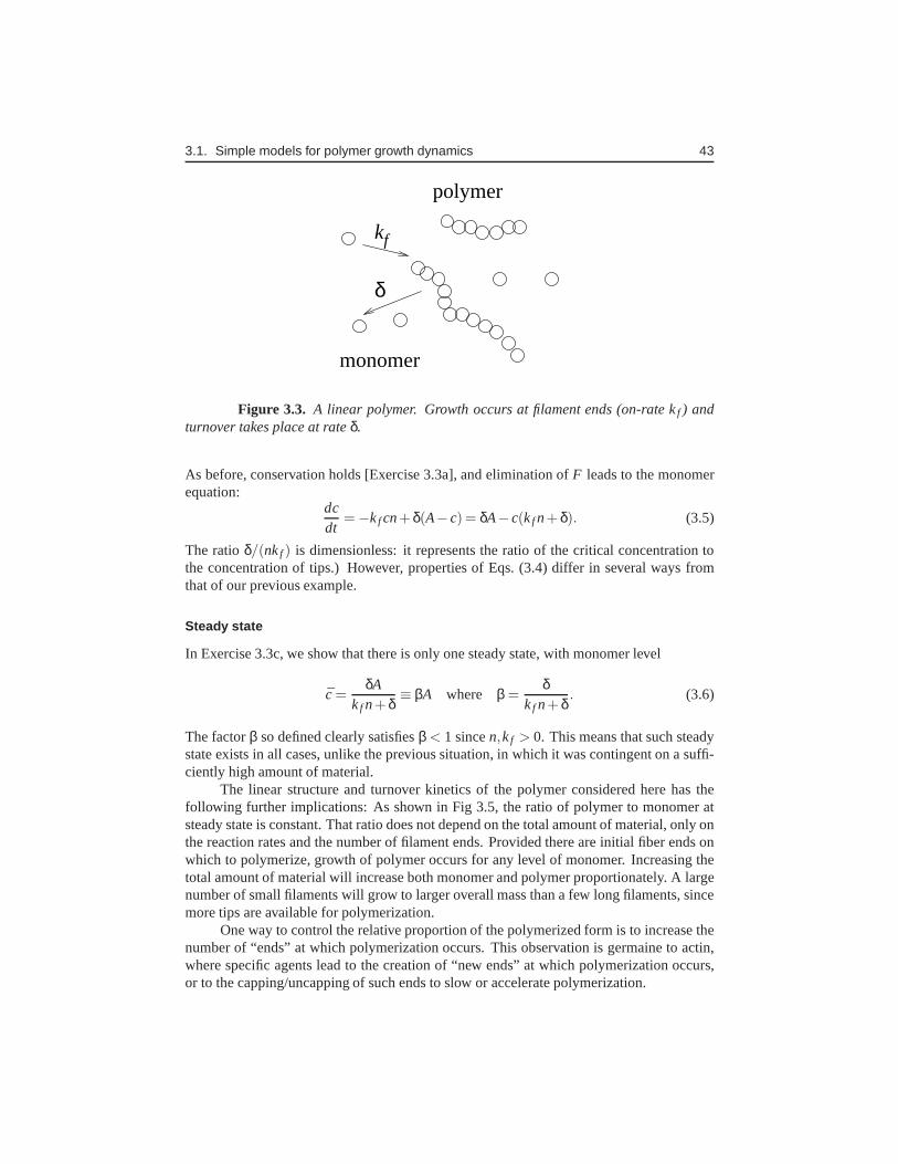
3.1. Simple models for polymer growth dynamics 43
δ
kf
monomer
polymer
Figure 3.3. A linear polymer. Growth occurs at filament ends (on-rate kf ) andturnover takes place at rateδ.
As before, conservation holds [Exercise 3.3a], and elimination of F leads to the monomerequation:
dcdt
=−kf cn+ δ(A− c) = δA− c(kf n+ δ). (3.5)
The ratioδ/(nkf ) is dimensionless: it represents the ratio of the critical concentration tothe concentration of tips.) However, properties of Eqs. (3.4) differ in several ways fromthat of our previous example.
Steady state
In Exercise 3.3c, we show that there is only one steady state,with monomer level
c=δA
kf n+ δ≡ βA where β =
δkf n+ δ
. (3.6)
The factorβ so defined clearly satisfiesβ < 1 sincen,kf > 0. This means that such steadystate exists in all cases, unlike the previous situation, inwhich it was contingent on a suffi-ciently high amount of material.
The linear structure and turnover kinetics of the polymer considered here has thefollowing further implications: As shown in Fig 3.5, the ratio of polymer to monomer atsteady state is constant. That ratio does not depend on the total amount of material, only onthe reaction rates and the number of filament ends. Provided there are initial fiber ends onwhich to polymerize, growth of polymer occurs for any level of monomer. Increasing thetotal amount of material will increase both monomer and polymer proportionately. A largenumber of small filaments will grow to larger overall mass than a few long filaments, sincemore tips are available for polymerization.
One way to control the relative proportion of the polymerized form is to increase thenumber of “ends” at which polymerization occurs. This observation is germaine to actin,where specific agents lead to the creation of “new ends” at which polymerization occurs,or to the capping/uncapping of such ends to slow or accelerate polymerization.

44 Chapter 3. Simple polymers
dc/dt
c0 A
0
0.5
1
1.5
2
2.5
3
0 2 4 6 8 10
Monomer
Polymer
(a) (b)
Figure 3.4. Polymerization kinetics in filament elongation with growthoccurringonly at filament tips, given by Eqs.(3.4). Here the number of tips, n is assumed to beconstant. (a) the flow is always towards a unique steady state, which is inside the domain.(b) time plot produced with XPP code (See Appendix A.B). Parameter values were kf =1,δ = 1,n= 5 and initial conditions were c(0) = 2.9,F(0) = 0.1
(b)
c
F
0ccrit
F
0c
(a)
Figure 3.5. Steady state values of polymer and monomer as the total amount ofmaterial A is slowly increased (direction of arrows). (a) Inthe case of simple aggregation,Eqs.(3.1), discussed in Section 3.1.1, for monomer concentration c= ccrit ≤ A no poly-merization will occur. Thereafter, the monomer level will be constant and excess materialwill all be incorporated into polymer. (b) In a linear polymer with irreversible addition ofmonomer only at filament ends as in Eqs.(3.4) of Section 3.1.2, there will be a constantratio of monomer and polymer. As A increases, both will increase. The slope of the line in(b) is nkf /δ. Increasing the number of filament tips, n, will mean that more of the materialis in polymer form.
A comparison of the steady state behaviour of the two models thus far considered isgiven in Fig. 3.5. Here we show the distinct predictions for steady state behaviour for thetwo distinct polymer types as the total amount of material,A is gradually increased.

3.1. Simple models for polymer growth dynamics 45
3.1.3 New tips are created and capped
New ends can be formed in a number of ways: (1) by spontaneous nucleation of filamentsfrom monomers (2) by breakage of long filaments to produce shorter ones with more ends,or (3) by agents that lead to branching of the filaments. We here concentrate on the thirdmechanism.
Assume that the filaments sprout new tips at some constant rate,φ. This allows poly-merization to accelerate. If new tips form without limit, nosteady state will be possible. Acontrol measure that limits explosive growth of new tips is needed, so we assume that thetips are capped at some rateκ. Kinetics of this type describe the polymerization of actininpresence of the nucleator Arp2/3 that leads to filament branching, and capping protein thatstalls elongation at some tips [17]. Then the system of interest is
dndt
= φF−κn, (3.7a)
dcdt
=−kf cn+ δF. (3.7b)
wherec is the monomer concentration 0≤ c ≤ A and F is filament length, as definedin Section 3.1.1. In Eqn. (3.7a) we see the creation of new tips along a filament (withrate φ per unit filament per unit time), and the first-order decay rate κn. In (3.7b) wehave monomer being used up at each tip (fueling the extensionof the filament) and beingrecycled from filament degradation. Note that tips do not carry a mass, as they are a site onan existing filament. The filament density equation is unchanged (here omitted), andF canbe eliminated (F = A− c) as before leading to
dndt
= φ(A− c)−κn, (3.8a)
dcdt
=−kf cn+ δ(A− c). (3.8b)
This is a system of two differential equations in the variablesn(t),c(t). whose time be-haviour is shown in the simulations of Fig 3.6. For low tip capping rateκ, the polymerwill form, as in Fig 3.6(a). Whenκ is too high, the filaments initially start to grow, buteventually decay, as shown in Fig 3.6(b).
This system can also be studied in thecn phase plane (Figure 3.7(a,b).) It is evidentthat there are up to two steady states,n = 0,c = A,F = 0 (unstable) and a stable steadystate at
c=δkf
κφ, F = A− c, n=
φκ
F,
that is physically meaningful only ifA > δκ/kf φ (Fig. 3.7(a)). If this inequality is notsatisfied, then only the trivial equilibrium is relevant andeventually, only monomer willremain (see Fig 3.7b and also Fig. 3.6b). In this sense, thereexists an “effective criticalconcentration”, whose value depends not only on the polymerization forward and backkinetics, but also on the creation and removal of tips that act as nucleation sites.

46 Chapter 3. Simple polymers
0
1
2
3
4
0 5 10 15 20
tips
polymer
monomer
t
0
1
2
3
0 5 10 15 20
monomer
polymer
tips
t
(a) (b)
Figure 3.6. Polymerization kinetics for the model(3.8) where new tips are cre-ated and capped. (a) For low capping rate,κ = 0.1 polymer is formed. (b) Forκ = 1,the polymerization cannot be sustained, and eventually, only monomers are left. Other pa-rameter values used were kf = 1,δ = 1,φ = 0.2,A= 3. Simulations done with XPP file inAppendix A.D. See also Fig 3.7 for another way to plot the sameinformation using aphaseplane diagram.
0
1
2
3
4
5
6
7
0 1 2 3
Stable S.S.
c nullcline
n nullcline
c
n
0
1
2
3
4
5
6
7
0 1 2 3
c nullcline
n nullclineStable S.S.
c
n
(a) (b)
Figure 3.7. Plane plots showing nullclines and steady states for the polymeriza-tion model in the case where filaments are broken to produce new tips, and tips are thencapped. The horizontal axis is c, and the vertical axis is n. See Fig 3.6 for the corre-sponding time plots. (a): For low capping rate,κ = 0.1 polymer is formed. (b):κ = 1,the polymerization cannot be sustained, and eventually, only monomers are left. Other pa-rameter values used were kf = 1,δ = 1,φ = 0.2,A= 3. See Section A.D for XPP file thatproduced these phase plane diagrams.

Exercises 47
QSS on filament ends
If new tips are formed and removed rapidly relative to other kinetics, than a QSS on thevariablen leads ton≈ (φ/κ)(A− c) so that
dcdt
=−kf cn+ δ(A− c) =−kf cφκ(A− c)+ δ(A− c)= kf (A− c)
(
δkf− φ
κc
)
(3.9)
Thus, the dynamics of this case is similar to those discussedin Section 3.1.1 in the limit ofrapid tip dynamics, but with a different “effective critical concentration”,c′crit = δκ/(kf φ).
3.1.4 Initial dynamics
The initial behaviour of this system starting withc≈ A, and someF = ε 6= 0 depends onwhether there are also exposed filament ends att = 0. There are two possibilities:
Case A: Some exposed tips at t = 0: In Fig 3.6, we illustrate the case wheren(0) 6= 0. InExercise 3.10b we ask the reader to show that close tot = 0, filaments grow linearly andtips grow quadratically.
Case B: No exposed tips at t = 0: If tips are initially all capped so thatn(0) = 0, then newtips must first form, before any polymerization can take place. In that case, close tot = 0,tips grow linearly and then filaments grow quadratically [Exercise 3.10c].
Implications
In this type of polymer reaction, with creation and capping of filament tips, either linearor quadratic initial polymerization rise time behaviour can occur. Washout decay is notchanged from the description in Section 3.1.2. The effective critical concentration in suchkinetics,c′crit = δκ/(kf φ), depends on turnover of both filaments and (exposed) tips, aswell as branching and monomer on-rate. This means that any one of these parameters caninfluence the long-term behaviour.
Exercises
3.1. (a) Show that the polymer equations (3.1) imply that thetotal amount of monomerand polymer are conserved.
(b) Verify the equation for the rate of change ofc obtained by eliminatingF .
(c) Explain how the diagram fordc/dt versusc is obtained from the differentialequation forc.
3.2. Use the XPP file provided in Appendix A.A to explore the polymerization by ag-gregation discussed in Section 3.1.1. Show that you get results as in Fig 3.2. Whatparameter(s) or value(s) should you vary to get the cases shown in panels (c) and (d)of that figure?

48 Chapter 3. Simple polymers
3.3. (a) Show that the polymer equations (3.4) imply that thetotal amount of monomerand polymer are conserved.
(b) Show thatF can be eliminated from Eqn. (3.4a) to arrive at Eqn (3.5).
(c) Show that (3.4) has a single steady state solution, and that the level of monomersat that steady state is given by (3.6). What is the corresponding level of poly-mer at that steady state?
(d) Show that if the number of “tips”,n, is constant, the steady state levels ofmonomer and polymer are proportional to each other.
3.4. Consider two special cases for the model (3.4) of polymer growing atn tips wheren> 0 is constant.
(a) First, consider the early time behaviour. Explain why this model implies thatsome polymer is needed initially so that further polymerization will occur.
(b) Assume that close to the beginning of the reaction,c≈ A, andF ≈ ε. Find theapproximate behaviour ofF(t) at this early time. Show thatdF/dt≈C so thatF grows linearly with time.
(c) What is the value of the constantC you found in part (b)?
(d) Now consider the case that monomer is continuously removed from a polymer-ized mix that had been at its steady state. What will happen tothe polymer?
3.5. Use the XPP code provided in Appendix A.B to explore the model for polymersgrowing at their tips discussed in Section 3.1.2. Show that you get the results givenin Fig 3.4. How does the behaviour change if there are more tips (n= 10)? If therate of growth is slower (kf = 0.2) ?
3.6. Consider modifications of the model (3.4) as follows:
(a) Show that if the polymerization at filament tips is reversible (with rate constantkr for loss of monomer from tips), then this shifts the steady state to
c=δA+ krnkf n+ δ
, F = A− c. (3.10)
(b) Show that if filaments do not turn over as a whole, but rather addand losemonomers at their ends, then the kinetics are different. Explore this model bysettingδ = 0 and replacingkf cnby (kf c− kr)n in the relevant equation.
(c) Show that the revision in (b) introduces a critical concentration,ccrit = kr/kf .
3.7. Consider Eqn. (3.3). What are the units of each of the variables? Suppose we definenew variables,t∗ = δt andc∗ = c/A whereA is the total amount of monomer in thesystem. (Note thatA,δ are positive constants carrying units. What are those units?)
(a) Explain why the new variables,t∗,c∗ are “dimensionless”, i.e. are unit-lessparameters.
(b) Substitutet = t∗/δ,c= c∗A into Eqn. (3.2) and simplify the equations. Showthat you obtain (after dropping the *’s).
dcdt
= (1−αc)(1− c). (3.11)
What is the value of the parameterα and what does it represent?

Exercises 49
(c) Use the results of analysis of Eqn. (3.3) to draw conclusions about the be-haviour of the dimensionless model, given by Eqn. (3.11).
3.8. For aggregating molecules, it may be the case that monomer addition or loss canonly occur from the surface of a dense growing “pellet”. Thiscase is a variationon the theme described in the model (3.1) of Section 3.1.1. Here we examine thisvariant.
(a) Since the variableF has units proportional to mass, and assuming a 3D (roughlyspherical) aggregate, show that the surface area of a singlepellet would be pro-portional toF2/3.
(b) Argue that this leads to the modified model
dcdt
= (−kf c+ δ)F2/3 = kf (A− c)2/3(
δkf− c
)
.
(c) Show that the steady state monomer and polymer level is unchanged in thissituation.
(d) Show that the initial growth (close tot = 0) and the “and washout kinetics”follow a power rather than exponential behaviour.
(e) Adapt the XPP code given in Section A.A to studying and characterizing thebehaviour of this variant of the model.
3.9. Consider the model (3.8) for polymer filaments with tipsthat are created and capped.
(a) What is the corresponding differential equation forF?
(b) Find the steady state(s) of (3.8).
(c) Draw the qualitative state space plot (analogous to Fig.3.2a,b) forc corre-sponding to the equation (3.9).
(d) For Eqn. (3.9), which steady statec is stable? (unstable?)
3.10. Consider the model (3.8) for polymer filaments with tips that are created and capped.
(a) Use the XPP file in Section A.D to simulate this model and recreate the timeplots shown in Fig 3.6.
(b) If n(0) 6= 0, show that close tot = 0, filaments grow linearly and tips growquadratically.
(c) If tips are initially all capped (n(0) = 0), show that close tot = 0, tips growlinearly and filaments grow quadratically.

50 Chapter 3. Simple polymers
Chapter 4
Introduction tonondimensionalization andscaling
This chapter is an introduction to the topic of dimensionless variables.
4.1 Simple examples
We start with simple models consisting of one differential equation in order to establishthe motivation in an elementary setting. We first discuss thelogistic population growthequation, and then move on to models in a chemical setting.
4.1.1 The logistic equation
A well-known model for the density-dependent growth of a populationN(t) is thelogisticequation ,
dNdt
= rN
(
1− NK
)
. (4.1)
Here r > 0 is the intrinsic growth rate in units of 1/time, andK > 0 is thecarryingcapacity, in the same units asN. This equation is a limited-growth version of theMalthusequation discussed in Exercise 4.??.
Dividing both sides byK and regrouping terms leads to
1K
dNdt
= rNK
(
1− NK
)
, ⇒ ddt
(
NK
)
= rNK
(
1− NK
)
. (4.2)
In this form, it is evident thatN only appears in in the groupingN/K. We can simplifythe equation and reduce the number of constants by treating this as a single new quantity.Accordingly, suppose we define a new variable,
y(t) =N(t)K
.
Note that in this form, the population is measured in “multiples” of the carrying capacity.Thusy is a pure number, a dimensionless variable carrying no units, even if originally we
51
52 Chapter 4. Introduction to nondimensionalization and scaling
had assigned units toN such as number of organisms per unit area of habitat. Making thesubstitutionN=Ky into Eqn (4.2) (or Eqn (4.1), for that matter), leads to the new equation,
dydt
= ry(1− y). (4.3)
We can go further with Eqn (4.3) and scale time so as to reduce the remaining parameter(r). To do so, we would define a new dimensionless variables= rt . Then the substitutiont = s/r into Eqn (4.3) will eliminate the remaining parameter, leading to
dyds
= y(1− y). (4.4)
[Details in Exercise 4.1]. This elementary first example already illustrates thatintroductionof dimensionless variables reduces the number of parameters that characterize a problem.Observe that in Eqn. (4.4), there are no free parameters left. This means that we canunderstand the essential behaviour of such an equation by studying this single prototyperather than considering all possible results for multiple values of the parametersr,K for theunscaled version, Eqn (4.1). The behaviour of Eqn. (4.4) is explored in Section??.
4.2 Other Examples
We present a few additional examples and show how each can be nondimensionalized. Herewe will also see steps to take when it is not immediately transparent which combinations ofchoices for scales are appropriate. Some of these examples arise in previous models (e.g.from Chapter 3) and others will be analyzed in later material.
Example 4.1 (Macrophages and dead cells). Find a dimensionless formulation for thefollowing set of equations arising in a model for macrophages (m(t)) removing dead cells(a(t)) and killing some cells in the process:
dmdt
= g · (M−m)a− km, (4.5a)
dadt
= κCm− f ma−da. (4.5b)
Here M and C are total numbers of macrophages and target cells, respectively, assumedto be constant in this example, and given in units such as cells cm−3 (i.e. cells per cubiccm). Time t is measured in hours. g is the rate of activation ofthe macrophages by deadcell material, k is the rate of inactivation.κ is the rate of “bystander” killing of cells, fis the rate of removal of dead cells by macrophages and d is some other turnover of deadcell material. It is assumed that g,k,κ, f ,d > 0 are constants. [See Exercise 4.3a for adiscussion of the units of these parameters.]
Solution. We assume the following scalings:
m= mm∗, a= aa∗, t = τt∗.

4.2. Other Examples 53
Herem, a,τ are constant (dimension carrying) scales, to be chosen, andm∗,a∗, t∗ are thenumerical (dimensionless) variables. Then, substitutingthis into Eqs. (4.5) leads to
d(mm∗)d(τt∗)
= g(M− mm∗)aa∗− kmm∗, (4.6a)
d(aa∗)d(τt∗)
= κCmm∗− f mm∗aa∗−daa∗. (4.6b)
We multiple both sides of Eqn. (4.6) byτ/m, and sides of Eqn. (4.8) byτ/a,
dm∗
dt∗=
τm[g(M− mm∗)aa∗− kmm∗] , (4.7a)
da∗
dt∗=
τa[κCmm∗− f mm∗aa∗−daa∗] . (4.7b)
Now distribute the terms and group constants and variable terms to obtain
dm∗
dt∗= gaτ((M/m)−m∗)a∗− kτm∗, (4.8a)
da∗
dt∗= κC
ma
τm∗− f τmm∗a∗−dτa∗. (4.8b)
Let us use square brackets to emphasize the groupings of constant terms:
dm∗
dt∗= [gaτ]([M/m]−m∗)a∗− [kτ]m∗, (4.9a)
da∗
dt∗=
[
κCma
τ]
m∗− [ f τm]m∗a∗− [dτ]a∗. (4.9b)
We select values for the constant scale so as to simplify as many of these groupings aspossible. In particular, we chose
[M/m] = 1,
[
κCma
τ]
= 1, [dτ] = 1.
This choice is, to some extent arbitrary in the current example. It implies that the convenientset of scales we have selected are
m= M, τ = 1/d, a= κCmτ =κCM
d.
We now drop the *s. The equations then simplify to
dmdt
= α(1−m)a− δm, (4.10a)
dadt
= m−ηma−a. (4.10b)
whereα = [gaτ], δ = [kτ] = k/d, η = [ f τm]. (4.11)

54 Chapter 4. Introduction to nondimensionalization and scaling
In Exercise 4.3b we ask the reader to rewrite these quantities in terms of the original pa-rameters of the problem and to interpret their meanings.
Example 4.2 (Predator Prey equations). Consider the following set of equations
dxdt
= r1x(
1− xK
)
−Axy
D+ x, (4.12a)
dydt
= r2y
(
1− yqx
)
. (4.12b)
These equations have been used to model the dynamics of interacting prey (x(t)) and preda-tors (y(t)). Assume that ri ,K,A,D,q> 0 are constants. Use dimensional analysis to reducethese to a dimensionless form.
Solution. We define the following scalings:
x= x x∗, y= yy∗, t = τt∗.
Here the quantities ¯x, y,τ are convenient “scales” that will be chosen shortly, as in theprevious example. They are constant, whereas the numericalvaluesx∗,y∗, t∗ that carry nodimensions are the variables. Substituting these assignments into Eqs. (4.12) leads to
dxx∗
dτt∗= r1xx∗
(
1− xx∗
K
)
−Axx∗yy∗
D+ xx∗, (4.13a)
dyy∗
dτt∗= r2yy∗
(
1− yy∗
qxx∗
)
. (4.13b)
We multiply both sides of Eqn. (4.13a) byτ/x and both sides of Eqn. (4.13b) byτ/y andsimplify to obtain:
dx∗
dt∗= [r1τ]x∗
(
1−[
xK
]
x∗)
−[
Aτyx
]
x∗y∗
[D/x]+ x∗, (4.14a)
dy∗
dt∗= [r2τ]y∗
(
1−[
yqx
]
y∗
x∗
)
. (4.14b)
[See Exercise 4.4b.] We now make judicious choices that reduce the complexity of theterms. We can chose the scales ¯x, y,τ, i.e. we have three independent choices to make. Itproves convenient to set
[r1τ] = 1,
[
xK
]
= 1,
[
yqx
]
= 1.
This is equivalent to selecting
τ = r1, x= K, y= qx= qK.
The equations are thereby simplified to
dx∗
dt∗= x∗ (1− x∗)−
[
Aτyx
]
x∗y∗
[D/x]+ x∗, (4.15a)
dy∗
dt∗= [r2τ]y∗
(
1− y∗
x∗
)
. (4.15b)
Exercises 55
We drop the *’s and obtain the final dimensionless set of equations
dxdt
= x(1− x)−αxy
δ+ x(4.16a)
dydt
= νy(
1− yx
)
(4.16b)
where the parameters in these have the following meanings:
α =
[
Aτyx
]
=Aqr1
, ν = [r2τ] =r2
r1, δ = [D/x] =
DK.
In Exercise 4.4c, we discuss the meanings of these parameters. We also consider an alter-nate rescaling in part (d) of the same exercise. We will studythis system further in a laterchapter. (See Eqns. (??) and their analysis in Chapter??.)
Exercises4.1. Consider the logistic equation (4.1).
(a) Explain why it must be true thatN(t) andK have the same units.
(b) SupposeN(t) is in units of density of organisms (e.g. number per unit area)and time is measured in years. What are the units of the termdN/dt? of r?What are the units of the quantity 1/r and how could this be interpreted?
(c) Now consider Eqn (4.3). Define a new variablet∗ = rt wherer is the growthrate. Show that the substitutiont = t∗/r into Eqn (4.3) will eliminate the re-maining parameter, leading to Eqn. (4.4). This is equivalent to rescaling timein units that have what meaning?
4.2. Suppose you have found a solutiony(t) to (4.4). Explain how you would convert thisto a solutionN(t) to (4.1). [Hint: consider a back substitution using the relationshipss= rt andy= N/K.]
4.3. (a) For the model of macrophages and target cells given by (4.5), if m andc haveunits of cells cm−3 (i.e. cells per cubic cm) and time is measured in hours,what are the units for each of the parametersg,k,κ, f ,d?
(b) Determine the values of the dimensionless parametersα,δ,η from (4.11) interms of the original parameters of the problem.
(c) Interpret the meanings of these dimensionless ratios.
4.4. Consider the model for predator-prey interactions given by (4.12). Suppose preda-tors and prey are both insects, and are measured in units of m−2 (e.g. number ofindividuals per square meter).
(a) What are the units of the parametersr i ,K,A,D,q?
(b) Verify the calculations resulting in (4.14).
(c) Interpret the meanings of the dimensionless ratiosα,ν,δ.
56 Chapter 4. Introduction to nondimensionalization and scaling
(d) Consider an alternate rescaling ¯x= y= K,τ = 1/A. Find the corresponding di-mensionless equations and dimensionless parameter groupings. Interpret yourresults.
4.5. Consider the following equations for the growth of a single species of organism:
dPdt
=vP
K+P−dP. (4.17)
(a) Interpret what these equations are saying.
(b) Definex= P/P,s= t/τ whereP,τ are scales to be chosen. Use substitution toconvert Eqn. (4.17) to a dimensionless form in terms of thesescales.
(c) What is a reasonable choice forP? For ,τ? Are there more than one possiblescalings that make sense for this model?
(d) Use an appropriate scaling to obtain a final dimensionless equations. Whatdimensionless parameter grouping(s) appear?
4.6. Consider the equationdxdt
= ax−bx3
(a) Show that this equation can be rescaled to the form
dxdt
= c
(
x− 13
x3)
by defining an appropriate scale ¯x for x.
(b) Show that by rescaling time, we arrive at a similar equation with c= 1.
See Section 1.0.1 for a further investigation of this cubic kinetics ODE.
4.7. Ludwig, Jones and Holling [9] studied the dynamics of the spruce budworm, heredenotedB(t). They suggested the following differential equation to describe thegrowth of these insects and predation by birds:
dBdt
= rBB
(
1− BKB
)
−βB2
α2+B2 . (4.18)
(a) Explain the meanings of the terms in this equation.
(b) Rewrite these equations in dimensionless form. There are two choices forscales for the budworm density and two for time.
4.8. Hasty et al [4] derived a model for the concentration of arepressorx(t) in the lysis-lysogeny pathway of theλ virus. A reduced version of this model is
dxdt
=AK1K2x2
1+(1+σ1K1K2x2+σ2K21K2
2x4)− kdx+ r (4.19)
Define a dimensionless repressor concentrationx∗ = x√
K1K2 and a dimensionlesstime t∗ = t(r
√K1K2). Show that the dimensionless equation can be written in the
formdxdt
=αx2
1+(1+σ1x2+σ2x4)− γx+1. (4.20)
Find the values of the parametersα,γ in terms of the original parameters.

Appendices
57


Appendix A
Appendix: XPP Files
Some instructions are provided here but readers who have never used XPP will find goodresources for the installation and usage of this freeware inan online tutorial by Ermentrout,as well as in his written accounts. An extensive guide, with many other interesting exam-ples, is [1]. A related text, also richly supported with XPP examples and instructions is[2].
A.A Simulation for simple aggregation of monomers
ODE file for Fig 3.2 in Section 3.1.1
# actin1.odedc/dt=-kf*c*F +kr*FdF/dt=kf*c*F -kr*Fparam kf=1, kr=1init c=0.7, F=0.1done
A.B Simulation for growth at filament tips
ODE file for Fig 3.4 in Section 3.1.2
# actin2.odedc/dt=-kf*c*n +kr*FdF/dt=kf*c*n -kr*Fparam kf=1, kr=1, n=5init c=2.9, F=0.1done
59

60 Appendix A. Appendix: XPP Files
A.B.1 Cubic kinetics
The following file was used to produce the solution curves of Fig. 1.0.1 and the bifurcationdiagram in Fig 1.4(b).
# cubic.ode## The cubic first order differential equation#x’= c*(x-(1/3)*xˆ3+A)param c=1,A=0done
In order to produce the bifurcation diagram follow these steps: Run the .ode file with initialx value 1.5 and type “Initial condition” “Last” (I L) to continue the solution so that it isextremely close to its steady state value (repeat I L two or three times to do this). Type“File” “Auto” (F A). This opens a new window. Edit the panels as follows: Parameter:there is only one parameter, so this need not be changed.Axes: select “hI-lo”. Then fillin the range Xmin = -2, Ymin= -3, Xmax=2, Ymax=3.Numerics: Change Par Min to -2,Par Max to 2, and Ds to 0.01. Press OK.Run: “Steady state”. This will produce part ofthe diagram starting with the value ofA = 0. To continue towards negative values ofA,grab one of the points, and edit the Numerics panel to change Ds to -0.01. This will run thecontinuation in the opposite direction. For more details, see the book by Bard Ermentrout[1].
A.B.2 Pitchfork bifurcations
The following file was used to produce the pitchfork bifurcation shown in Fig. 1.9.
# Pitchfork.odex’=r*x-xˆ3param r=-0.5init x=0done
Instructions: Run the file in auto for some time steps. SelectF (File) A (Auto). Theparameter will already be set tor, as that is the only parameter in the problem. Select Axes,hI-lo, and set Xmin:-0.1, Ymin:-1, Xmax: 0.25, Ymax 1. Select Numerics and change ParMin: -0.5, Par Max: 0.25. click OK, then Run: Steady state.
To produce the subcritical pitchfork bifurcation of Fig. 1.9, the file used was
# PitchforkSub.ode
x’=r*x+xˆ3
param r=0.2init x=0done
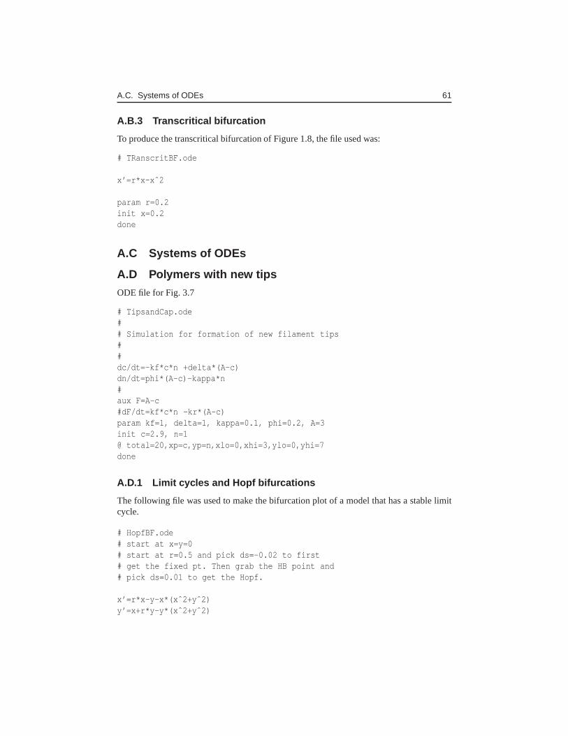
A.C. Systems of ODEs 61
A.B.3 Transcritical bifurcation
To produce the transcritical bifurcation of Figure 1.8, thefile used was:
# TRanscritBF.ode
x’=r*x-xˆ2
param r=0.2init x=0.2done
A.C Systems of ODEs
A.D Polymers with new tips
ODE file for Fig. 3.7
# TipsandCap.ode## Simulation for formation of new filament tips##dc/dt=-kf*c*n +delta*(A-c)dn/dt=phi*(A-c)-kappa*n#aux F=A-c#dF/dt=kf*c*n -kr*(A-c)param kf=1, delta=1, kappa=0.1, phi=0.2, A=3init c=2.9, n=1@ total=20,xp=c,yp=n,xlo=0,xhi=3,ylo=0,yhi=7done
A.D.1 Limit cycles and Hopf bifurcations
The following file was used to make the bifurcation plot of a model that has a stable limitcycle.
# HopfBF.ode# start at x=y=0# start at r=0.5 and pick ds=-0.02 to first# get the fixed pt. Then grab the HB point and# pick ds=0.01 to get the Hopf.
x’=r*x-y-x*(xˆ2+yˆ2)y’=x+r*y-y*(xˆ2+yˆ2)
62 Appendix A. Appendix: XPP Files
param r=0.5init x=0,y=0done
The equations were integrated first with the above initial conditions. In Auto, the Numericssettings were changed as follows: ds: -0.02, Parmin:-0.5, Parmax: 2. Then select Run:Steady state. This produced the line of fixed point with bifurcation point atr = 0. Theoption Grab and tab key selects that bifurcation point. Hit Return. In the Numerics panel,switch to ds:0.01, then Run Periodic.
# HopfsubBF.ode# start at x=y=0# pick ds=-0.02 to get steady state# then grab HB point and Run Periodic
x’=r*x-y+x*(xˆ2+yˆ2)y’=x+r*y+y*(xˆ2+yˆ2)
param r=0.5init x=0,y=0done
Auto was run in a similar way, but the direction of steps ds need not be changed. The opendots signify an unstable limit cycle.
A.E Fitzhugh Nagumo Equations
#FitzhughNagumo1.ode# file to produce simulations for FHN model
dx/dt = c*(x-(xˆ3)/3-y+j)dy/dt = (x+a-b*y)/c
aux v=-x
par j=0,a=0.7,b=0.8,c=3# Consider either c=3 or c=10# Parameters should satisfy 1-(2/3)b<a<1, 0<b<1
# Convenient initial conditions:init x=2.0,y=2.0
@ total=20,xp=x,yp=y,dt=0.01,xlo=-3,xhi=2,ylo=-1,yhi =2done
Now let us make the bifurcation diagram shown in Fig??. To do so, setj = 0 and inte-grate the equations to get as close as possible to the (stable) steady state. (e.g. use Initial

A.F. Lysis-Lysogeny ODE model (Hasty et al) 63
Conditions, Mouse [I M] to start close to the nullcline intersection, then continue usingInitial Conditions, Last [I L] to get even closer. Start autoby clicking File, Auto [F A]and set the Axes to hI-Lo with Xmin:0, Ymin:-2,Xmax:1,Ymax:2. In the Numerics panelchange Par Min:0 Par Max:1, click OK, and Run Steady state. You will get the horizontalbranch of steady state, with a bifurcation point (HB). Grab that point and Run periodic(after decreasing ds to 0.005) to get this picture.
A.F Lysis-Lysogeny ODE model (Hasty et al)The following XPP file was used to produce Figs. 2.12 for the Lysis-Lysogeny model.
# lysislysogeny.ode# Based on eq 7 in Hasty et al PNAS (2000) vol 97 #5 2075-2080# should have a bistable switch# gamma is the bifurcation parameter (range gamma= 14-16)#x’= alpha*xˆ2/(1+(1+sigma1)*xˆ2+sigma2*xˆ4)-gamma*x+ 1param gamma=18,alpha=50,sigma1=1,sigma2=5@total=10,xlo=0,xhi=10,ylo=0,yhi=1done
To generate the bifurcation diagram5, first integrate the ODE file starting fromx= 0 a fewtimes to get as close as possible to the steady statexss= 0.06845. (e.g., integrate, then“Continue” till t = 500, which does the job. Start Auto (File, Auto). Select Axes, hI-lo,Xmin:10, Ymin:0, Xmax:20, Ymax:1 [Note that gamma will be onthe horizontal axis, andxss on the vertical axis.] Select Numerics, and change only Ds:-0.02, Dsmax:0.1,Par Min:0, Par Max: 20. (Click OK.) Select Run, Steady state. This will produce the Bifurcationplot.
A.G Simple biochemical modules
A.G.1 Production and Decay
The following XPP file was used to produce the production-decay behaviour in Fig. 2.2(a)
# ASProdDecay.ode# Simple signal for production and decay of substance#R’=k0+k1*S-k2*R
# Signal gets turned on at time 0, off at time 3# uses "Heaviside" step function to turn on or off
S=heav(t-0)-heav(t-3)
5I want to thank Bard Ermentrout for helping me with the Auto settings for this file. L.E.K.
64 Appendix A. Appendix: XPP Files
param k0=1,k1=1,k2=1init R=1@total=10done
A.G.2 Adaptation
The following XPP file was used to produce the adaptation behaviour in Fig. 2.2(b)
# AdaptTyson.ode# An adaptation circuit#R’=k1*S-k2*X*RX’=k3*S-k4*X
# Signal gets turned up in steps at times t=0, 5, 10, 15# uses "Heaviside" step function
S=heav(t-0)+heav(t-5)+heav(t-10)+heav(t-15)
param k1=1,k2=1, k3=1, k4=2init R=1, X=0.5@total=10done
A.G.3 Genetic toggle switch
The following XPP file was used to produce the switch-like behaviour of Fig. 2.6
# AToggleSwitch.ode## Based on Gardner et al Nature (2000) Vol 403 pp 339-342# By making either n or m large enough, get# nonlinearity that produces multiple steady states# and a switch-like response#u’=alpha1/(1+vˆn)-uv’=alpha2/(1+uˆm)-vparam alpha1=3,alpha2=3,n=3, m=3@ total=20,xp=u,yp=v,dt=0.01,xlo=0,xhi=4,ylo=0,yhi=4done

A.H. Cell division cycle models 65
A.H Cell division cycle models
A.H.1 The simplest Novak-Tyson model (Eqs. (2.21))
The following XPP file was used to produce the phase plane of Fig 2.12 and the bifurcationdiagram in Fig. 2.13.
# tysonCCJTB01.ode# Model based on first system (eqs 2) shown in Tyson’s paper# JTB (2001) vol 210 pp 249-263# Y=[CycB] = cyclin cdk dimers# P=[Cdh1]= APN Cdh1 complex (proteolytic complex)# Y and P are mutually antagonistic
Y’=k1-(k2p+k2pp*P)*YP’=Factiv(P)*(1-P)-Fdecay(Y,P)*P
Factiv(P)=(k3p+k3pp*A)/(J3+1-P)Fdecay(Y,P)=k4*m*Y/(J4+P)
# parameters with units of 1/time:par k1=0.04par k2p=0.04,k2pp=1par k3p=1,k3pp=10par k4=35par A=0
# mass of cell (try m=0.6, m=0.3)par m=0.3
# Dimensionless parameters:par J3=0.04,J4=0.04
@ dt=0.005@ xp=Y,yp=P,xlo=0,xhi=1,ylo=0,yhi=1done
To make an AUTO bifurcation diagram, the system was first started with the parameterm= 0.1, and integrated for many time steps to arrive at the steady statey= 0.038684p=0.99402.m was used as the bifurcation parameter. Auto Axes were set as hI-lo, with Y onthe Y-axis, and Main Parm:m on the horizontal axis, and with Xmin:0, Ymin:0, Xmax:0.6,Ymax:1.5.
This system was slightly fiddly, and a few first attempts at producing a bifurcationdiagram with the default AUTO numerics parameters were unsuccessful (MX type error).
AutoNumerics parameters were adjusted as follows:Ntst:50, Nmax:200, NPr:50,Ds:0.002, Dsmin: 0.0001, Ncol:4, EPSL:0.0001, Dsmax:0.5,Par Min: 0.1, Par Max: 0.2,Norm min:0, Norm Max: 1000, EPSU: 0.001, EPSS:0,001. The diagram was built up

66 Appendix A. Appendix: XPP Files
gradually by increasing the range of the plotted curve.
A.H.2 The second Novak-Tyson model
The following file was used to simulate theAY phase plane plots in Fig 2.14(a)-2.14(c).Note that hereP is put on QSS.
# tysonCCJTB01_3QSSP.ode
# Model based on three eqns system (eqs 3) shown in Tyson’s pap er# JTB (2001) vol 210 pp 249-263
# Y=[CycB] = cyclin cdk dimers# P=[Cdh1]= APN Cdh1 complex (proteolytic complex)# Y and P are mutually antagonistic# A= Cdc14=Cdc20 - eqn (3) in this paper# In this file we put P on QSS and look at Y and A
Y’=k1-(k2p+k2pp*P)*Y
#P’=Factiv(P)*(1-P)-Fdecay(Y,P)*P#Factiv(P)=(k3p+k3pp*A)/(J3+1-P)#Fdecay(Y,P)=k4*m*Y/(J4+P)
P=G((k3p+k3pp*A)/(k4*m),Y,J3,J4)
# Here is the Goldbeter-Koshland function that comes# from solving dP/dt=0G(Va,Vi,Ja,Ji)=2*Va*Ji/(Vi-Va+Va*Ji+Vi*Ja+ sqrt((Vi- Va+Va*Ji+Vi*Ja)ˆ2-4*(Vi-Va)*Va*Ji))
A’=k5p+k5pp* ((m*Y/J5)ˆn)/(1+(y*m/J5)ˆn)-k6*A
# parameters with units of 1/time:par k1=0.04par k2p=0.04,k2pp=1par k3p=1,k3pp=10par k4=35par k5p=0.005,k5pp=0.2,k6=0.1
# mass of cell (try m=1, m=0.3)par m=0.3
# Dimensionless parameters:par J3=0.04,J4=0.04,J5=0.3,n=4

A.H. Cell division cycle models 67
@ dt=0.005@ xp=A,yp=Y,xlo=0,xhi=1,ylo=0,yhi=1done
A.H.3 The three-variable YPAmodel
The amended file below was used to produce Fig. 2.15 in Section2.6.1.
#tyson.ode# Equations
# EquationsY’=k1-(k2p+k2pp*P)*YP’=(1-P)*(k3p+k3pp*A)/(J3+1-P)-P*k4*m*Y/(J4+P)A’=k5p+k5pp* ((m*Y/J5)ˆn)/(1+(y*m/J5)ˆn)-k6*A
# Parameters with units of 1/time:p k1=0.04p k2p=0.04,k2pp=1p k3p=1,k3pp=10p k4=35p k5p=0.005,k5pp=0.2,k6=0.1
# mass of cell (try m=0.6, m=0.3, m=1)p m=1
# Dimensionless parameters:p J3=0.04,J4=0.04,J5=0.3,n=4# Numerics@ TOTAL=2000,DT=.1,xlo=0,xhi=2000,ylo=0,yhi=6@ NPLOT=1,XP1=t,YP1=Y@ MAXSTOR=10000000@ BOUNDS=100000@ dsmin=1e-5,dsmax=.1,parmin=-.5,parmax=.5,autoxmin= -.5,autoxmax=.5@ autoymax=.4,autoymin=-.5
# ICY(0)=1P(0)=0.5A(0)=0.1done
To make the bifurcation diagram shown in Fig. 2.15, follow the procedure below.
• Change the integration method to ”STIFF” (nUmerics, Method, Stiff, return, escape).
68 Appendix A. Appendix: XPP Files
• First ’Initial condition’, ’Go’, we can get some periodic graph at the bottom of thedrawing area. Click two peaks of the graph to find the approximate the period of thesolution. It is about 56.45.
• ’numerics’—change ’total’: 56.45, ’dt’:0.05, escape.
• erase the original graph, ’IL’ several time to make sure to get closer and closer to theexact stable period orbit.
• open the auto window. Select the auto settings as follows:’Parameter’—’Par1’: m;’Axes’—’hilo’— ’Xmax’: 30, ’Ymax’: 5;’Numerics’—’Ntst’:60,’Nmax’:200,’Npr’:500,’Epsl’: 0.000001, ’ParMax’:30;
• ’Run’—’Periodic’, two short lines appears in the left bottom corner, if necessary,click ’abort’ to stop them.;
• ’Grab’ and enter.
• ’Numerics’—’Ds’:-0.02.
• ’Run’—’extend’, you will find the both two ends will extend, but it takes a long time,so if necessary, click ’abort’ to stop them.
• Then we want to find the steady state. Before we do that, ’file’—’clear grab’.
• Go back to Xpp, ’Parameter’—m:10, and ’IL’ several times.
• Go back to Auto, and ’Run’—’Steady State’, a window will appear to ask youwhether want to destroy the diagram, choose ’No’, a fancy S-shaped graph will beadded to the diagram (lighter than the original one).
• To see them more clearly, ’Axes’—’fit’, ’redraw’. You might get a graph with somespace between the first set of darker lines and lighter S-shaped curve, depending onhow long you run before you click ’abort’ when you run the extension.
• ’Axes’—’fit’,’redraw’, the the former two darker line are averaged.
• There is more interesting behaviour for smaller values ofm. To see these, click file,clear grab, and go back to XPP window. Changem to 0.3, and resimulate (InitialCond, Go, I L,I L,I L, I L). Return to AUTO windo, and reset the numerics so thatParmin=0.3, Parmax = 2. Run. This will allow you to see the fold bifurction. Thereis also a subcritical Hopf bifurcation atm= 0.5719. You can see this by grabbingthe Hopf point, adjusting the numerics menu to get Parmin=0.2, Parmax=0.6 andrunning the periodic.
• The last graph is the same as ’Tyson.ps’.

A.H. Cell division cycle models 69
0
0.1
0.2
0.3
0.4
0.5
0.6
0.7
0.8
0.9
Y
1 2 3 4 5 6 7 8 9 10
m
(a)
0.1
0.2
0.3
0.4
0.5
0.5 1 1.5 2 2.5
m
Y
(b)
Figure A.1. Bifurcation diagram for the full YPA model given by Eqs.(2.24)(b)A zoom into part of the diagram of (a). See also Fig 2.15 for another zoomed view.
A.H.4 A more complete cell cycle model
The file below was used to produce Fig 2.19. in Section 2.6.2.
# tysonCCJTB01_4.ode
# Model based on three eqns system (eqs 3) shown in Tyson’s pap er# JTB (2001) vol 210 pp 249-263
# Y=[CycB] = cyclin cdk dimers# P=[Cdh1]= APN Cdh1 complex (proteolytic complex)# Y and P are mutually antagonistic# A= Cdc14=Total Cdc20 - eqn (3) in this paper#AA = active Cdc20 = Cdc20_A eqn (4)# IP = [IAP] eqn(5)
Y’=k1-(k2p+k2pp*P)*YP’=Factiv(P)*(1-P)-Fdecay(Y,P)*P
######NOTE: CHANGE IN THE FOLLOWING FORMULA A->AA# as per Tyson’s discussion on p 255
Factiv(P)=(k3p+k3pp*AA)/(J3+1-P)Fdecay(Y,P)=k4*m*Y/(J4+P)
A’=k5p+k5pp* ((m*Y/J5)ˆn)/(1+(y*m/J5)ˆn)-k6*A
AA’ = k7*IP*(A-AA)/(J7+A-AA) -k6*AA -k8*Mad*AA/(J8+AA)

70 Appendix A. Appendix: XPP Files
IP’=k9*m*Y*(1-IP)-k10*IP
m’= mu*m*(1-m/ms)
# parameters with units of 1/time:par k1=0.04par k2p=0.04,k2pp=1par k3p=1,k3pp=10par k4=35par k5p=0.005,k5pp=0.2,k6=0.1
par k7=1,k8=0.5,Mad=1par k9=0.1,k10=0.02par mu=0.01,ms=10
#Global flag: See XPP book p 36# When Y falls below threshold, the cell divides,# then its mass m is 1/2 its previous mass.global -1 Y-Ythresh {m=m/2}par Ythresh=0.1
# mass of cell (try m=0.6, m=0.3)#par m=0.3
# Dimensionless parameters:par J3=0.04,J4=0.04,J5=0.3,n=4par J7=0.001,J8=0.001
init Y=0.6,P=0.02,A=1.6,AA=0.6,IP=0.6,m=0.8
@ dt=0.005,Total=300,MAXSTOR=500000,BACK= {White}done
A.I Odell-Oster model
The following XPP file can be used to investigate the Oster-Odell cell contraction model.
#Odell.ode# file to produce simulations for Oster and Odell (1984) mode l
L’=k*(L0*1/(Cˆ2+C0)-L)C’=g*L-v*C+a*Cˆ2/(b+Cˆ2)
par k=1,L0=0.1,g=1,v=1,a=2.3,b=1.5,C0=0.5@ total=20,xp=C,yp=L,xlo=0,xhi=2,ylo=0,yhi=0.3done

Bibliography
[1] Bard Ermentrout,Simulating, analyzing, and animating dynamical systems, SIAM,Philadelphia, 2002.
[2] C.P. Fall, E.S. Marland, J.M. Wagner, and J.J. Tyson,Computational cell biology,Springer, New York, 2002.
[3] T.S. Gardner, C.R. Cantor, and J.J. Collins,Construction of a genetic toggle switch inEscherichia coli, Nature403 (2000), no. 6767, 339–342.
[4] J. Hasty, J. Pradines, M. Dolnik, and JJ Collins,Noise-based switches and amplifiersfor gene expression, Proceedings of the National Academy of Sciences of the UnitedStates of America97 (2000), no. 5, 2075.
[5] P.A. Iglesias and A. Levchenko,Modeling the cell’s guidance system, Science’s STKE2002 (2002), no. 148.
[6] B.N. Kholodenko,Negative feedback and ultrasensitivity can bring about oscillationsin the mitogen-activated protein kinase cascades, European Journal of Biochemistry267 (2000), no. 6, 1583–1588.
[7] , Cell-signalling dynamics in time and space, Nature Reviews Molecular CellBiology 7 (2006), no. 3, 165–176.
[8] A. Levchenko and P.A. Iglesias,Models of eukaryotic gradient sensing: applicationto chemotaxis of amoebae and neutrophils, Biophysical journal82 (2002), no. 1, 50–63.
[9] D. Ludwig, D.D. Jones, and CS Holling,Qualitative analysis of insect outbreak sys-tems: the spruce budworm and forest, The Journal of Animal Ecology47 (1978),no. 1, 315–332.
[10] N.I. Markevich, J.B. Hoek, and B.N. Kholodenko,Signaling switches and bistabilityarising from multisite phosphorylation in protein kinase cascades, The Journal of CellBiology 164 (2004), no. 3, 353.
[11] H Naiki and F Gejyo,Kinetic analysis of amyloid fibril formation., Methods Enzymol309 (1999), 305–318 (eng).
71
72 Bibliography
[12] B. Novak and J.J. Tyson,Quantitative analysis of a molecular model of mitotic controlin fission yeast, J. theoret. Biol.173 (1995), 283–305.
[13] G. Odell, G. Oster, P. Alberch, and B. Burnside,The mechanical basis of morphogen-esis. I. Ephitelial folding and invagination, Dev. Biol.85 (1981), 446–462.
[14] R.J. Prill, P.A. Iglesias, and A. Levchenko,Dynamic properties of network motifscontribute to biological network organization, PLoS biology3 (2005), no. 11, 1881.
[15] H.M. Sauro and B.N. Kholodenko,Quantitative analysis of signaling networks,Progress in biophysics and molecular biology86 (2004), no. 1, 5–43.
[16] S.H. Strogatz,Nonlinear dynamics and chaos: With applications to physics, biology,chemistry, and engineering, Westview Pr, 2000.
[17] T M Svitkina and G G Borisy,Arp2/3 complex and actin depolymerizing factor/cofilinin dendritic organization and treadmilling of actin filament array in lamellipodia., JCell Biol 145 (1999), no. 5, 1009–1026 (eng).
[18] J.J. Tyson, K. Chen, and B. Novak,Sniffers, buzzers, toggles and blinkers: dynamicsof regulatory and signaling pathways in the cell, Current Opinion in Cell Biology15(2003), no. 2, 221–231.
[19] J.J. Tyson and B. Novak,Regulation of the eukaryotic cell cycle: molecular antag-onism, hysteresis, and irreversible transitions, Journal of Theoretical Biology210(2001), no. 2, 249–263.
[20] J.J. Tyson, B. Novak, K. Chen, and J. Val,Checkpoints in the cell cycle from a mod-eler’s perspective, Progress in Cell Cycle Res. (L. Meijer, S. Guidet, and H.Y.L. Tung,eds.), vol. 1, Plenum Press, New York, 1995, pp. 1–8.
[21] J.J. Tyson, B. Novak, G.M. Odell, K. Chen, and C.D. Thron, Chemical kinetic theory:understanding cell-cycle regulation, TIBS 21 (1996), 89–96.
Index
adapt, 16autocatalysis, 3
bifurcation, 2subcritical pitchfork, 5diagram, 2fold, 4, 25parameter, 2pitchfork, 5plot, 21points, 6saddle-node, 25transcritical, 4value, 3, 4
bistability, 18, 21bistable
kinetics, 1branched
polymer, 40
carrying capacity, 51checkpoint, 22conservation, 14continuation
methods, 3cooperative
kinetics, 3cooperativity, 19critical
concentration, 40
derivativesign of, 40
dimer, 3, 19
E. coli, 17extremum, 5
foldbifurcation, 3, 4
G1, 22gap, 22genetic
switch, 19Goldbeter-Koshland
function, 15, 26growth rate
intrinsic, 51
Hillconstant, 3function, 3
Hopf bifurcationsubcritical, 28, 29
hysteresis, 25
kinase, 23
LEGI, 16limit cycle
unstable, 28logistic
equation, 51
Malthusequation, 51
maximumlocal, 5
minimumlocal, 5
mitosis, 22
parameterreduction, 52
phase
73

74 Index
line, 8phosphatase, 23pitchfork bifurcation, 5polymer
branched, 39population
growth, 51
QSS, 26, 36
saddle-nodebifurcation, 4
saddle-node/loopbifurcation, 28–30
second derivativetest, 5
sigmoidalfunction, 3
steady state, 40subcritical
pitchfork bifurcation, 5synthesis, 22
tipcapping, 45
toggle switch, 17transcription factor, 19transcritical bifurcation, 4
variabledimensionless, 51
virus, 19


