NOTES ON DESIGN AND ANALYSIS OF ALGORITHMS B.TECH II …

DESIGN AND ANALYSIS OF ALGORITHMS Page 1

NOTES

ON

DESIGN AND ANALYSIS OF ALGORITHMS

B.TECH II YEAR - II SEM (2017-18)

DEPARTMENT OF INFORMATION TECHNOLOGY

MALLA REDDY COLLEGE ENGINEERING

(Autonomous)

Maisammaguda, Dhulapally (Post Via. Hakimpet), Secunderabad – 500100, Telangana State, INDIA.



SYLLABUS

Objectives:

To analyze performance of algorithms.

To choose the appropriate data structure and algorithm design method for a

specified application.

To understand how the choice of data structures and algorithm design

methods impacts the performance of programs.

To solve problems using algorithm design methods such as the greedy

method, divide and conquer, dynamic programming, backtracking and branch

and bound.

Prerequisites (Subjects) Data structures, Mathematical foundations of

computer science.

MODULE I:

Introduction: Algorithm, Psuedo code for expressing algorithms, Performance Analysis-

Space complexity, Time complexity, Asymptotic Notation- Big oh notation, Omega notation,

Theta notation and Little oh notation, Probabilistic analysis, Amortized analysis.

Divide and conquer: General method, applications-Binary search, Quick sort, Merge sort,

Strassen’s matrix multiplication.

MODULE II:

Searching and Traversal Techniques: Efficient non - recursive binary tree traversal

algorithm, Disjoint set operations, union and find algorithms, Spanning trees, Graph traversals

- Breadth first search and Depth first search, AND / OR graphs, game trees, Connected

Components, Bi - connected components. Disjoint Sets- disjoint set operations, union and

find algorithms, spanning trees, connected components and biconnected components.

MODULE III:

Greedy method: General method, applications - Job sequencing with deadlines, 0/1 knapsack

problem, Minimum cost spanning trees, Single source shortest path problem. Dynamic

Programming: General method, applications-Matrix chain multiplication, Optimal binary

search trees, 0/1 knapsack problem, All pairs shortest path problem, Travelling sales person

problem, Reliability design.


MODULE IV:

Backtracking: General method, applications-n-queen problem, sum of subsets problem, graph

coloring, Hamiltonian cycles.

Branch and Bound: General method, applications - Travelling sales person problem,0/1

knapsack problem- LC Branch and Bound solution, FIFO Branch and Bound solution.

MODULE V:

NP-Hard and NP-Complete problems: Basic concepts, non deterministic algorithms, NP - Hard

and NPComplete classes, Cook’s theorem.

TEXT BOOKS:

1. Fundamentals of Computer Algorithms, Ellis Horowitz,Satraj Sahni and

Rajasekharam,Galgotia publications pvt. Ltd.

2. Foundations of Algorithm, 4th edition, R. Neapolitan and K. Naimipour, Jones and Bartlett

Learning.

3. Design and Analysis of Algorithms, P. H. Dave, H. B. Dave, Pearson Education, 2008.

REFERENCES:

1. Computer Algorithms, Introduction to Design and Analysis, 3rd Edition, Sara Baase, Allen, Van,

Gelder, Pearson Education.

2. Algorithm Design: Foundations, Analysis and Internet examples, M. T. Goodrich and

R. Tomassia, John Wiley and sons.

3. Fundamentals of Sequential and Parallel Algorithm, K. A. Berman and J. L. Paul, Cengage

Learning.

4. Introducation to the Design and Analysis of Algorithms, A. Levitin, Pearson Education.

5. Introducation to Algorithms, 3rd Edition, T. H. Cormen, C. E. Leiserson, R. L. Rivest, and C. Stein,

PHI Pvt. Ltd.

6. Design and Analysis of algorithm, Aho, Ullman and Hopcroft, Pearson Education, 2004.

Outcomes:

Be able to analyze algorithms and improve the efficiency of algorithms. Apply different designing methods for development of algorithms to realistic problems, such

as divide and conquer, greedy and etc. Ability to understand and estimate the performance of

algorithm.



INDEX

S. No MODULE

Topic Page no

1

I Introduction to Algorithms 5

2

I Divide and Conquer 24

3

II Searching and Traversal Techniques 42

4

III Greedy Method 54

5

III Dynamic Programming 67

6

IV Back Tracking 102

7

IV Branch and Bound 114

8

V NP-Hard and NP-Complete Problems 133

9


MODULE I:

Introduction: Algorithm, Psuedo code for expressing algorithms, Performance Analysis- Space

complexity, Time complexity, Asymptotic Notation- Big oh notation, Omega notation, Theta

notation and Little oh notation, Probabilistic analysis, Amortized analysis.

Divide and conquer: General method, applications-Binary search, Quick sort, Merge sort,


INTRODUCTION TO ALGORITHM

History of Algorithm

• The word algorithm comes from the name of a Persian author, Abu Ja’far Mohammed ibn Musa al

Khowarizmi (c. 825 A.D.), who wrote a textbook on mathematics. • He is credited with providing the step-by-step rules for adding, subtracting, multiplying, and

dividing ordinary decimal numbers. • When written in Latin, the name became Algorismus, from which algorithm is but a small step • This word has taken on a special significance in computer science, where “algorithm” has come to

refer to a method that can be used by a computer for the solution of a problem • Between 400 and 300 B.C., the great Greek mathematician Euclid invented an algorithm

• Finding the greatest common divisor (gcd) of two positive integers. • The gcd of X and Y is the largest integer that exactly divides both X and Y . • Eg.,the gcd of 80 and 32 is 16.

• The Euclidian algorithm, as it is called, is considered to be the first non-trivial algorithm ever devised.

What is an Algorithm?

Algorithm is a set of steps to complete a task.

For example,

Task: to make a cup of tea.

Algorithm: · add water and milk to the kettle,

· boil it, add tea leaves,

· Add sugar, and then serve it in cup.

‘’a set of steps to accomplish or complete a task that is described precisely enough that a

computer can run it’’.

Described precisely: very difficult for a machine to know how much water, milk to be added

etc. in the above tea making algorithm.

These algorithms run on computers or computational devices..For example, GPS in our

smartphones, Google hangouts.

GPS uses shortest path algorithm.. Online shopping uses cryptography which uses RSA algorithm.

• Algorithm Definition1:


• An algorithm is a finite set of instructions that, if followed, accomplishes a particular task. In

addition, all algorithms must satisfy the following criteria:

• Input. Zero or more quantities are externally supplied.

• Output. At least one quantity is produced.

• Definiteness. Each instruction is clear and unambiguous.

• Finiteness. The algorithm terminates after a finite number of steps.

• Effectiveness. Every instruction must be very basic enough and must be feasible.

• Algorithm Definition2:

• An algorithm is a sequence of unambiguous instructions for solving a problem, i.e., for obtaining a

required output for any legitimate input in a finite amount of time.

• Algorithms that are definite and effective are also called computational procedures. • A program is the expression of an algorithm in a programming language

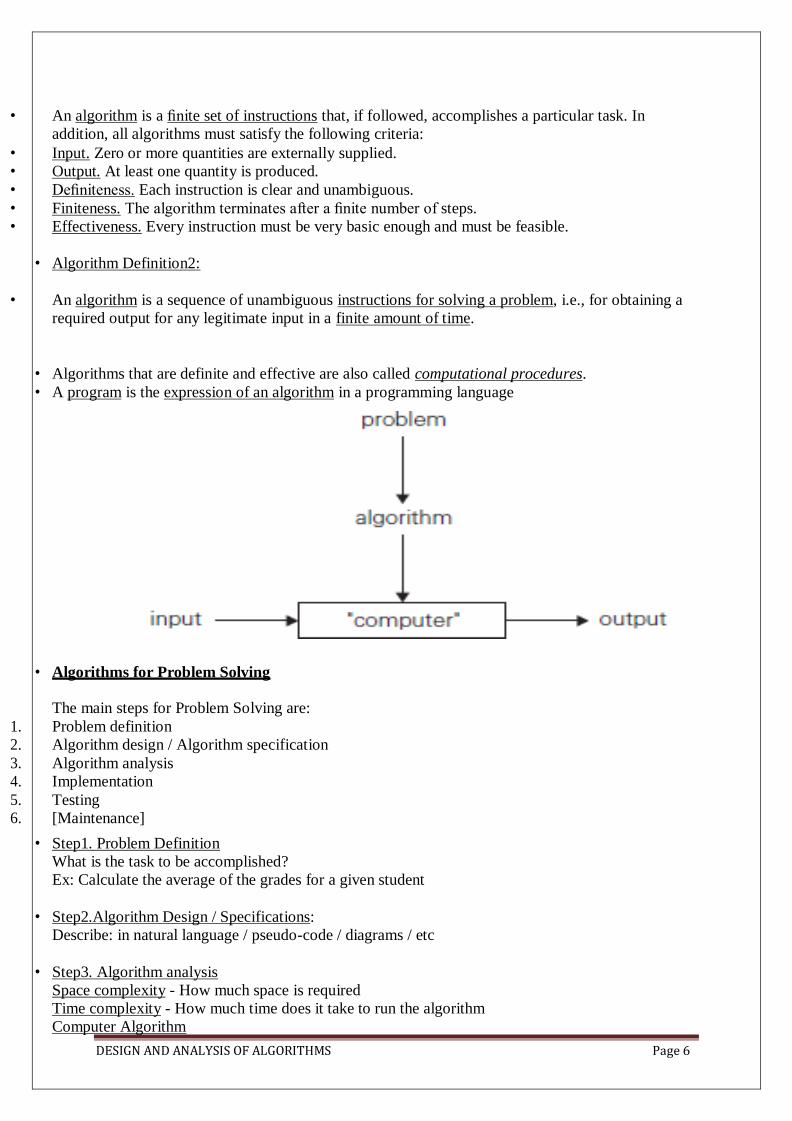
• Algorithms for Problem Solving

The main steps for Problem Solving are:

1. Problem definition

2. Algorithm design / Algorithm specification

3. Algorithm analysis

4. Implementation

5. Testing

6. [Maintenance]

• Step1. Problem Definition What is the task to be accomplished?

Ex: Calculate the average of the grades for a given student

• Step2.Algorithm Design / Specifications: Describe: in natural language / pseudo-code / diagrams / etc

• Step3. Algorithm analysis Space complexity - How much space is required

Time complexity - How much time does it take to run the algorithm

Computer Algorithm


An algorithm is a procedure (a finite set of well-defined instructions) for accomplishing some tasks

which, given an initial state terminate in a defined end-state

The computational complexity and efficient implementation of the algorithm are important in computing,

and this depends on suitable data structures.

• Steps 4,5,6: Implementation, Testing, Maintainance • Implementation:

Decide on the programming language to use C, C++, Lisp, Java, Perl, Prolog, assembly, etc.

, etc.

Write clean, well documented code

• Test, test, test

Integrate feedback from users, fix bugs, ensure compatibility across different versions

• Maintenance.

Release Updates,fix bugs

Keeping illegal inputs separate is the responsibility of the algorithmic problem, while treating

special classes of unusual or undesirable inputs is the responsibility of the algorithm itself.


• 4 Distinct areas of study of algorithms:

• How to devise algorithms. Techniques – Divide & Conquer, Branch and Bound , Dynamic

Programming

• How to validate algorithms. • Check for Algorithm that it computes the correct answer for all possible legal inputs.

algorithm validation. First Phase

• Second phase Algorithm to Program Program Proving or Program Verification Solution be stated in two forms:

• First Form: Program which is annotated by a set of assertions about the input and output variables of

the program predicate calculus

• Second form: is called a specification • 4 Distinct areas of study of algorithms (..Contd) • How to analyze algorithms.

• Analysis of Algorithms or performance analysis refer to the task of determining how much

computing time & storage an algorithm requires • How to test a program 2 phases

• Debugging - Debugging is the process of executing programs on sample data sets to determine

whether faulty results occur and, if so, to correct them. • Profiling or performance measurement is the process of executing a correct program on data sets and

measuring the time and space it takes to compute the results

PSEUDOCODE:

• Algorithm can be represented in Text mode and Graphic mode

• Graphical representation is called Flowchart • Text mode most often represented in close to any High level language such as C,

PascalPseudocode

• Pseudocode: High-level description of an algorithm. • More structured than plain English.

• Less detailed than a program. • Preferred notation for describing algorithms. • Hides program design issues.

• Example of Pseudocode:

• To find the max element of an array

Algorithm arrayMax(A, n)

Input array A of n integers

Output maximum element of A

currentMax A[0]

for i 1 to n 1 do

if A[i] currentMax then

currentMax A[i]


• Control flow • if … then … [else …] • while … do … • repeat … until … • for … do … • Indentation replaces braces • Method declaration • Algorithm method (arg [, arg…])

• Input … • Output …

• Method call • var.method (arg [, arg…]) • Return value • return expression • Expressions

• Assignment (equivalent to )

• Equality testing (equivalent to ) • n2 Superscripts and other mathematical formatting allowed

PERFORMANCE ANALYSIS:

• What are the Criteria for judging algorithms that have a more direct relationship to performance? • computing time and storage requirements.

• Performance evaluation can be loosely divided into two major phases: • a priori estimates and • a posteriori testing. • refer as performance analysis and performance measurement respectively

• The space complexity of an algorithm is the amount of memory it needs to run to completion.

• The time complexity of an algorithm is the amount of computer time it needs to run to completion.

Space Complexity:

• Space Complexity Example:

• Algorithm abc(a,b,c) { return a+b++*c+(a+b-c)/(a+b) +4.0;

}

The Space needed by each of these algorithms is seen to be the sum of the following

component.

1.A fixed part that is independent of the characteristics (eg:number,size)of the inputs and

outputs.

The part typically includes the instruction space (ie. Space for the code), space for simple variable

and fixed-size component variables (also called aggregate) space for constants, and so on.

return currentMax


2. A variable part that consists of the space needed by component variables whose size is

dependent on the particular problem instance being solved, the space needed by referenced

variables (to the extent that is depends on instance characteristics), and the recursion stack space.

The space requirement s(p) of any algorithm p may therefore be written as, S(P) =

c+ Sp(Instance characteristics)

Where ‘c’ is a constant.

Example 2:

Algorithm sum(a,n) { s=0.0;

for I=1 to n do s=

s+a[I]; return s;

}

The problem instances for this algorithm are characterized by n,the number of

elements to be summed. The space needed d by ‘n’ is one word, since it is of type

integer.

The space needed by ‘a’a is the space needed by variables of tyepe array of

floating point numbers.

This is atleast ‘n’ words, since ‘a’ must be large enough to hold the ‘n’

elements to be summed.

So,we obtain Ssum(n)>=(n+s)

• [ n for a[],one each for n,I a& s]

Time Complexity:

• The time T(p) taken by a program P is the sum of the compile time and the

run time(execution time)

• The compile time does not depend on the instance characteristics. Also we may

assume that a compiled program will be run several times without recompilation .This rum

time is denoted by tp(instance characteristics).

• The number of steps any problem statement is assigned depends on the kind of statement.

• For example, comments à 0 steps.

Assignment statements is 1 steps.


[Which does not involve any calls to other algorithms]

Interactive statement such as for, while & repeat-untilà Control part of the statement.

We introduce a variable, count into the program statement to increment count with initial

value 0.Statement to increment count by the appropriate amount are introduced into the

program.

This is done so that each time a statement in the original program is executes count

is incremented by the step count of that statement.

Algorithm:

Algorithm sum(a,n) {

s= 0.0;

count = count+1; for I=1

to n do

{

count =count+1;

s=s+a[I];

count=count+1;

}

count=count+1;

count=count+1; return

s;

}

If the count is zero to start with, then it will be 2n+3 on termination. So each

invocation of sum execute a total of 2n+3 steps.

2. The second method to determine the step count of an algorithm is to build a table

in which we list the total number of steps contributes by each statement.

First determine the number of steps per execution (s/e) of the statement and the total

number of times (ie., frequency) each statement is executed.

By combining these two quantities, the total contribution of all statements, the step

count for the entire algorithm is obtained.

Statement Steps per execution

Frequency Total

1. Algorithm Sum(a,n)

2.{

3. S=0.0;

4. for I=1 to n do 5.

s=s+a[I];

6. return s;

7. }

0 0

1

1

1

1

0

- - 1

n+1 n 1

-

0 0

1

n+1 n 1

0

Total 2n+3


How to analyse an Algorithm?

Let us form an algorithm for Insertion sort (which sort a sequence of numbers).The pseudo code

for the algorithm is give below.

Pseudo code for insertion Algorithm:

Identify each line of the pseudo code with symbols such as C1, C2 ..

PSeudocode for Insertion Algorithm Line Identification

for j=2 to A length C1

key=A[j] C2

//Insert A[j] into sorted Array A[1. ..... j-1] C3

i=j-1 C4

while i>0 & A[j]>key C5

A[i+1]=A[i] C6

i=i-1 C7

A[i+1]=key C8

Let Ci be the cost of ith line. Since comment lines will not incur any cost C3=0.

Cost No. Of times

Executed

C1 N

C2 n-1

C3=0 n-1

C4 n-1

C5

C6

C7

C8 n-1

Running time of the algorithm is:

T(n)=C1n+C2(n-1)+0(n-1)+C4(n-1)+C5( )+C6(

)+C7(

)+

C8(n-1)

Best case:

It occurs when Array is sorted. All tj

values are 1.


T(n)=C1n+C2(n-1)+0 (n-1)+C4(n-1)+C5( ) +C6( )+C7( )+

C8(n-1)

=C1n+C2 (n-1) +0 (n-1) +C4 (n-1) +C5 + C8 (n-1)

= (C1+C2+C4+C5+ C8) n-(C2+C4+C5+ C8)

· Which is of the form an+b.

· Linear function of n.

So, linear growth.

Worst case:

It occurs when Array is reverse sorted, and tj =j

T(n)=C1n + C2(n-1)+0 (n-1)+C4(n-1)+C5( ) +C6( )+C7( ) +

C8(n-1)

=C1n+C2(n-1)+C4(n-1)+C5( ) +C6(

)+C7(

)+ C8(n-1)

which is of the form an2+bn+c

Quadratic function. So in worst case insertion set grows in n2. Why

we concentrate on worst-case running time?

· The worst-case running time gives a guaranteed upper bound on the running time for

any input.

· For some algorithms, the worst case occurs often. For example, when searching, the

worst case often occurs when the item being searched for is not present, and searches for

absent items may be frequent.

· Why not analyze the average case? Because it’s often about as bad as the worst case.

Order of growth:

It is described by the highest degree term of the formula for running time. (Drop lower-order terms.

Ignore the constant coefficient in the leading term.)

Example: We found out that for insertion sort the worst-case running time is of the form an2 +

bn + c.

Drop lower-order terms. What remains is an2.Ignore constant coefficient. It results in n2.But we

cannot say that the worst-case running time T(n) equals n2 .Rather It grows like n2 . But it doesn’t

equal n2.We say that the running time is Θ (n2) to capture the notion that the order of growth is n2.


We usually consider one algorithm to be more efficient than another if its worst-case

running time has a smaller order of growth.

Complexity of Algorithms

The complexity of an algorithm M is the function f(n) which gives the running time and/or storage

space requirement of the algorithm in terms of the size ‘n’ of the input data. Mostly, the storage

space required by an algorithm is simply a multiple of the data size ‘n’.

Complexity shall refer to the running time of the algorithm.

The function f(n), gives the running time of an algorithm, depends not only on the size ‘n’ of the

input data but also on the particular data. The complexity function f(n) for certain cases are:

1. Best Case : The minimum possible value of f(n) is called the best case.

2. Average Case : The expected value of f(n).

3. Worst Case : The maximum value of f(n) for any key possible input.

ASYMPTOTIC NOTATION

Formal way notation to speak about functions and classify them

The following notations are commonly use notations in performance analysis and used to

characterize the complexity of an algorithm:

1. Big–OH (O) ,

2. Big–OMEGA (Ω),

3. Big–THETA (Θ) and

4. Little–OH (o)

Asymptotic Analysis of Algorithms:

Our approach is based on the asymptotic complexity measure. This means that we don’t try to count

the exact number of steps of a program, but how that number grows with the size of the input to the

program. That gives us a measure that will work for different operating systems, compilers and

CPUs. The asymptotic complexity is written using big-O notation.

· It is a way to describe the characteristics of a function in the limit.

· It describes the rate of growth of functions.

· Focus on what’s important by abstracting away low-order terms and constant factors.

· It is a way to compare “sizes” of functions: O≈ ≤


Ω≈ ≥ Θ ≈ = o ≈ < ω

≈ >

Time complexity Name Example

O(1) Constant Adding an element to the front of a linked list

O(logn) Logarithmic Finding an element in a sorted array

O (n) Linear Finding an element in an unsorted array

O(nlog n) Linear Logarithmic Sorting n items by ‘divide-and-conquer’-

Mergesort

O(n2) Quadratic Shortest path between two nodes in a graph

O(n3) Cubic Matrix Multiplication

O(2n) Exponential The Towers of Hanoi problem

Big ‘oh’: the function f(n)=O(g(n)) iff there exist positive constants c and no such that

f(n)<=c*g(n) for all n, n>= no.

Omega: the function f(n)=(g(n)) iff there exist positive constants c and no such that f(n)

>= c*g(n) for all n, n >= no.

Theta: the function f(n)=(g(n)) iff there exist positive constants c1,c2 and no such that c1 g(n)

<= f(n) <= c2 g(n) for all n, n >= no

Big-O Notation

This notation gives the tight upper bound of the given function. Generally we represent it as f(n) =

O(g (11)). That means, at larger values of n, the upper bound off(n) is g(n). For example, if f(n) = n4

+ 100n2 + 10n + 50 is the given algorithm, then n4 is g(n). That means g(n) gives the maximum rate

of growth for f(n) at larger values of n.

O —notation defined as O(g(n)) = {f(n): there exist positive constants c and no such that 0 <=

f(n) <= cg(n) for all n >= no}. g(n) is an asymptotic tight upper bound for f(n). Our objective is to

give some rate of growth g(n) which is greater than given algorithms rate of growth f(n).

In general, we do not consider lower values of n. That means the rate of growth at lower values of n

is not important. In the below figure, no is the point from which we consider the rate of growths for a

given algorithm. Below no the rate of growths may be different.


Note Analyze the algorithms at larger values of n only What this means is, below no we do not

care for rates of growth.

Omega— Ω notation

Similar to above discussion, this notation gives the tighter lower bound of the given

algorithm and we represent it as f(n) = Ω (g(n)). That means, at larger values of n, the

tighter lower bound of f(n) is g

For example, if f(n) = 100n2 + 10n + 50, g(n) is Ω (n2).

The . Ω. notation as be defined as Ω (g (n)) = {f(n): there exist positive constants c and no

such that 0 <= cg (n) <= f(n) for all n >= no}. g(n) is an asymptotic lower bound for f(n). Ω (g

(n)) is the set of functions with smaller or same order of growth as f(n).

Theta- Θ notation

This notation decides whether the upper and lower bounds of a given function are same or not. The

average running time of algorithm is always between lower bound and upper bound.


If the upper bound (O) and lower bound (Ω) gives the same result then Θ notation will also have the

same rate of growth. As an example, let us assume that f(n) = 10n + n is the expression. Then, its

tight upper bound g(n) is O(n). The rate of growth in best case is g (n) = 0(n). In this case, rate of

growths in best case and worst are same. As a result, the average case will also be same.

None: For a given function (algorithm), if the rate of growths (bounds) for O and Ω are not same

then the rate of growth Θ case may not be same.

Now consider the definition of Θ notation It is defined as Θ (g(n)) = {f(71): there exist positive

constants C1, C2 and no such that O<=5 c1g(n) <= f(n) <= c2g(n) for all n >= no}. g(n) is an

asymptotic tight bound for f(n). Θ (g(n)) is the set of functions with the same order of growth as

g(n).

Important Notes

For analysis (best case, worst case and average) we try to give upper bound (O) and lower bound

(Ω) and average running time (Θ). From the above examples, it should also be clear that, for a

given function (algorithm) getting upper bound (O) and lower bound (Ω) and average running

time (Θ) may not be possible always.

For example, if we are discussing the best case of an algorithm, then we try to give upper bound

(O) and lower bound (Ω) and average running time (Θ).

In the remaining chapters we generally concentrate on upper bound (O) because knowing lower

bound (Ω) of an algorithm is of no practical importance and we use 9 notation if upper bound (O)

and lower bound (Ω) are same.

Little Oh Notation

The little Oh is denoted as o. It is defined as : Let, f(n} and g(n} be the non negative functions

then


such that f(n}= o(g{n)} i.e f of n is little Oh of g of n.

f(n) = o(g(n)) if and only if f'(n) = o(g(n)) and f(n) != Θ {g(n))

PROBABILISTIC ANALYSIS

Probabilistic analysis is the use of probability in the analysis of problems.

In order to perform a probabilistic analysis, we must use knowledge of, or make assumptions about,

the distribution of the inputs. Then we analyze our algorithm, computing an average- case running

time, where we take the average over the distribution of the possible inputs.

Basics of Probability Theory

Probability theory has the goal of characterizing the outcomes of natural or conceptual

“experiments.” Examples of such experiments include tossing a coin ten times, rolling a die three

times, playing a lottery, gambling, picking a ball from an urn containing white and red balls, and so

on

Each possible outcome of an experiment is called a sample point and the set of all possible outcomes

is known as the sample space S. In this text we assume that S is finite (such a sample space is called

a discrete sample space). An event E is a subset of the sample space S. If the sample space consists

of n sample points, then there are 2n possible events.

Definition- Probability: The probability of an event E is defined to be

where S is the

sample space.

Then the indicator random variable I {A} associated with event A is defined as I {A}

= 1 if A occurs ;

0 if A does not occur

The probability of event E is denoted as Prob. [E] The complement of E, denoted E, is defined to be

S - E. If E1 and E2 are two events, the probability of E1 or E2 or both happening is denoted as

Prob.[E1 U E2]. The probability of both E1 and E2 occurring at the same time is denoted as

Prob.[E1 0 E2]. The corresponding event is E1 0 E2.

Theorem 1.5

1. Prob.[E] = 1 - Prob.[E].

2. Prob.[E1 U E2] = Prob.[E1] + Prob.[E2] - Prob.[E1 ∩ E2]

<= Prob.[E1] + Prob.[E2]

Expected value of a random variable


The simplest and most useful summary of the distribution of a random variable is the average”

of the values it takes on. The expected value (or, synonymously, expectation or mean) of a

discrete random variable X is

E[X] =

which is well defined if the sum is finite or converges absolutely.

Consider a game in which you flip two fair coins. You earn $3 for each head but lose $2 for each

tail. The expected value of the random variable X representing

your earnings is

E[X] = 6.Pr{2H’s} + 1.Pr{1H,1T} – 4 Pr{2T’s}

= 6(1/4)+1(1/2)-4(1/4)

=1

Any one of these first i candidates is equally likely to be the best-qualified so far. Candidate i has a

probability of 1/i of being better qualified than candidates 1 through i -1 and thus a probability of 1/i

of being hired.

E[Xi]= 1/i

So,

E[X] = E[ ]

AMORTIZED ANALYSIS

In an amortized analysis, we average the time required to perform a sequence of datastructure

operations over all the operations performed. With amortized analysis, we can show that the average

cost of an operation is small, if we average over a sequence of operations, even though a single

operation within the sequence might be expensive. Amortized analysis differs from average-case

analysis in that probability is not involved; an amortized analysis guarantees the average

performance of each operation in the worst case.

Three most common techniques used in amortized analysis:

1. Aggregate Analysis - in which we determine an upper bound T(n) on the total cost of a sequence

of n operations. The average cost per operation is then T(n)/n. We take the average cost as the

amortized cost of each operation

2. Accounting method – When there is more than one type of operation, each type of operation may

have a different amortized cost. The accounting method overcharges some operations early in the

sequence, storing the overcharge as “prepaid credit” on specific objects in the data structure. Later

in the sequence, the credit pays for operations that are charged less than they actually cost.

= =


3. Potential method - The potential method maintains the credit as the “potential energy” of the

data structure as a whole instead of associating the credit with individual objects within the data

structure. The potential method, which is like the accounting method in that we determine the

amortized cost of each operation and may overcharge operations early on to compensate for

undercharges later

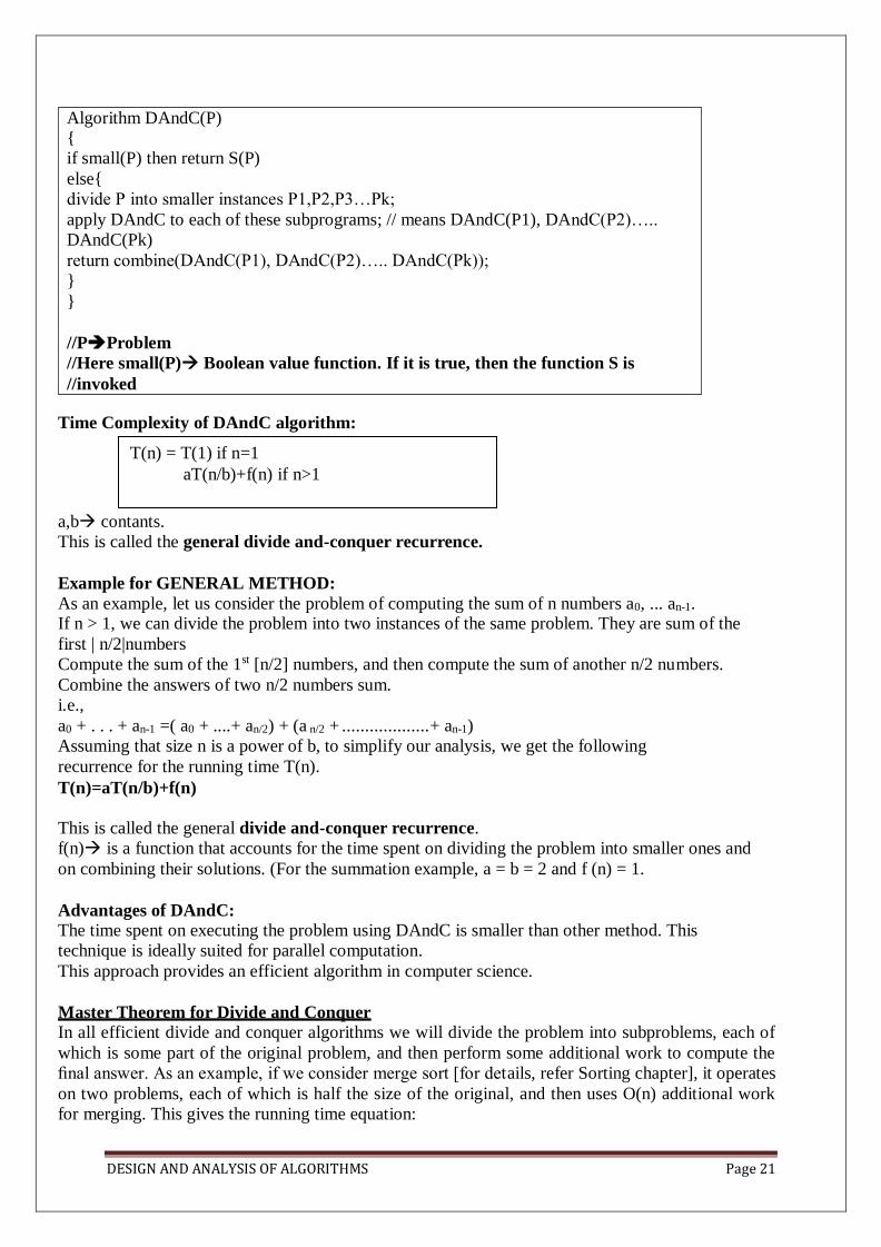
DIVIDE AND CONQUER

General Method

In divide and conquer method, a given problem is,

i) Divided into smaller subproblems.

ii) These subproblems are solved independently.

iii) Combining all the solutions of subproblems into a solution of the whole.

If the subproblems are large enough then divide and conquer is reapplied. The

generated subproblems are usually of some type as the original problem.

Hence recurssive algorithms are used in divide and conquer strategy.

Subprogram of size

Solution to Solution to

Solution to the original problem of

Subprogram of size

Problem of size N

Pseudo code Representation of Divide and conquer rule for problem “P”


Time Complexity of DAndC algorithm:

a,b contants.

This is called the general divide and-conquer recurrence.

Example for GENERAL METHOD:

As an example, let us consider the problem of computing the sum of n numbers a0, ... an-1. If n > 1, we can divide the problem into two instances of the same problem. They are sum of the

first | n/2|numbers

Compute the sum of the 1st [n/2] numbers, and then compute the sum of another n/2 numbers.

Combine the answers of two n/2 numbers sum.

i.e.,

a0 + . . . + an-1 =( a0 + ....+ an/2) + (a n/2 + ................... + an-1)

Assuming that size n is a power of b, to simplify our analysis, we get the following

recurrence for the running time T(n).

T(n)=aT(n/b)+f(n)

This is called the general divide and-conquer recurrence.

f(n) is a function that accounts for the time spent on dividing the problem into smaller ones and

on combining their solutions. (For the summation example, a = b = 2 and f (n) = 1.

Advantages of DAndC:

The time spent on executing the problem using DAndC is smaller than other method. This

technique is ideally suited for parallel computation.

This approach provides an efficient algorithm in computer science.

Master Theorem for Divide and Conquer

In all efficient divide and conquer algorithms we will divide the problem into subproblems, each of

which is some part of the original problem, and then perform some additional work to compute the

final answer. As an example, if we consider merge sort [for details, refer Sorting chapter], it operates

on two problems, each of which is half the size of the original, and then uses O(n) additional work

for merging. This gives the running time equation:

Algorithm DAndC(P) {

if small(P) then return S(P)

else{

divide P into smaller instances P1,P2,P3…Pk;

apply DAndC to each of these subprograms; // means DAndC(P1), DAndC(P2)…..

DAndC(Pk)

return combine(DAndC(P1), DAndC(P2)….. DAndC(Pk));

}

}

//PProblem

//Here small(P) Boolean value function. If it is true, then the function S is

//invoked

T(n) = T(1) if n=1

aT(n/b)+f(n) if n>1


T(n) = 2T( )+ O(n)

The following theorem can be used to determine the running time of divide and conquer

algorithms. For a given program or algorithm, first we try to find the recurrence relation for the

problem. If the recurrence is of below form then we directly give the answer without fully solving

it.

If the reccurrence is of the form T(n) = aT( ) + Θ (nklogpn), where a >= 1, b > 1, k >= O

and p is a real number, then we can directly give the answer as:

1) If a > bk, then T(n) = Θ (

)

2) If a = bk

a. If p > -1, then T(n) = Θ ( )

b. If p = -1, then T(n) = Θ ( )

c. If p < -1, then T(n) = Θ ( s)

3) If a < bk

a. If p >= 0, then T(n) = Θ (nklogpn)

b. If p < 0, then T(n) = 0(nk)

Applications of Divide and conquer rule or algorithm:

Binary search, Quick sort,

Merge sort,


Binary search or Half-interval search algorithm:

1. This algorithm finds the position of a specified input value (the search "key") within an array

sorted by key value.

2. In each step, the algorithm compares the search key value with the key value of the middle

element of the array.

3. If the keys match, then a matching element has been found and its index, or position, is returned.

4. Otherwise, if the search key is less than the middle element's key, then the algorithm repeats its

action on the sub-array to the left of the middle element or, if the search key is greater, then the

algorithm repeats on sub array to the right of the middle element.

5. If the search element is less than the minimum position element or greater than the maximum

position element then this algorithm returns not found.

Binary search algorithm by using recursive methodology:

Program for binary search (recursive) Algorithm for binary search (recursive) int binary_search(int A[], int key, int imin, int imax) Algorithm binary_search(A, key, imin, imax)

http://en.wikipedia.org/wiki/Sorted_array

http://en.wikipedia.org/wiki/Sorted_array


{

if (imax < imin)

return array is empty;

if(key<imin || K>imax)

return element not in array list else

{

int imid = (imin +imax)/2; if

(A[imid] > key)

return binary_search(A, key, imin, imid-1); else

if (A[imid] < key)

return binary_search(A, key, imid+1, imax); else

return imid;

}

}

{

if (imax < imin) then

return “array is empty”;

if(key<imin || K>imax) then

return “element not in array list”

else

{

imid = (imin +imax)/2; if

(A[imid] > key) then

return binary_search(A, key, imin, imid-1);

else if (A[imid] < key) then

return binary_search(A, key, imid+1, imax); else

return imid;

}

}

Time Complexity:

Data structure:- Array For successful search Unsuccessful search

Worst case O(log n) or θ(log n)

Average case O(log n) or θ(log n) Best case O(1) or θ(1)

θ(log n):- for all cases.

Binary search algorithm by using iterative methodology:

Binary search program by using iterative

methodology:

Binary search algorithm by using iterative

methodology:

int binary_search(int A[], int key, int imin, int

imax)

{

while (imax >= imin)

{

int imid = midpoint(imin, imax);

if(A[imid] == key)

return imid;

else if (A[imid] < key) imin

= imid + 1;

else

imax = imid - 1;

}

}

Algorithm binary_search(A, key, imin, imax)

{

While < (imax >= imin)> do

{

int imid = midpoint(imin, imax);

if(A[imid] == key)

return imid;

else if (A[imid] < key) imin

= imid + 1;

else

imax = imid - 1;

}

}

Merge Sort: The merge sort splits the list to be sorted into two equal halves, and places them in separate arrays. This

sorting method is an example of the DIVIDE-AND-CONQUER paradigm i.e. it breaks the data into two

halves and then sorts the two half data sets recursively, and finally merges them to obtain the complete

sorted list. The merge sort is a comparison sort and has an algorithmic complexity of O (n log n).

Elementary implementations of the merge sort make use of two arrays - one for each half of the data set.

The following image depicts the complete procedure of merge sort.


Advantages of Merge Sort:

1. Marginally faster than the heap sort for larger sets

2. Merge Sort always does lesser number of comparisons than Quick Sort. Worst case for merge sort

does about 39% less comparisons against quick sort’s average case.

3. Merge sort is often the best choice for sorting a linked list because the slow random- access

performance of a linked list makes some other algorithms (such as quick sort) perform poorly, and

others (such as heap sort) completely impossible.

Program for Merge sort:

#include<stdio.h>

#include<conio.h>

int n;

void main(){

int i,low,high,z,y;

int a[10];

void mergesort(int a[10],int low,int high);

void display(int a[10]);

clrscr();

printf("\n \t\t mergesort \n");

printf("\n enter the length of the list:");

scanf("%d",&n);

printf("\n enter the list elements");

for(i=0;i<n;i++)

scanf("%d",&a[i]);

low=0;

high=n-1;

mergesort(a,low,high);

display(a);

getch();

} void mergesort(int a[10],int low, int high)


{

int mid;

void combine(int a[10],int low, int mid, int high);

if(low<high)

{

mid=(low+high)/2;

mergesort(a,low,mid);

mergesort(a,mid+1,high);

combine(a,low,mid,high);

}

}

void combine(int a[10], int low, int mid, int high){ int

i,j,k;

int temp[10];

k=low; i=low;

j=mid+1;

while(i<=mid&&j<=high){

if(a[i]<=a[j])

{

temp[k]=a[i]; i++;

k++;

}

else

{

temp[k]=a[j]; j++;

k++;

}

}

while(i<=mid){

temp[k]=a[i]; i++;

k++;

}

while(j<=high){

temp[k]=a[j]; j++;

k++;

}

for(k=low;k<=high;k++)

a[k]=temp[k];

}

void display(int a[10]){ int i;

printf("\n \n the sorted array is \n");

for(i=0;i<n;i++)

printf("%d \t",a[i]);}


Algorithm for Merge sort:

Algorithm mergesort(low, high) { if(low<high) then // Dividing Problem into Sub-problems and { this “mid” is for finding where to split the set. mid=(low+high)/2;

mergesort(low,mid);

mergesort(mid+1,high); //Solve the sub-problems

Merge(low,mid,high); // Combine the solution

}

}

void Merge(low, mid,high){

k=low;

i=low;

j=mid+1;

while(i<=mid&&j<=high) do{

if(a[i]<=a[j]) then

{

temp[k]=a[i];

i++;

k++;

}

else

{

temp[k]=a[j];

j++;

k++;

}

}

while(i<=mid) do{

temp[k]=a[i];

i++;

k++;

}

while(j<=high) do{

temp[k]=a[j];

j++;

k++;

}

For k=low to high do

a[k]=temp[k];

}

For k:=low to high do a[k]=temp[k];

}


sive calls e of recu all of Me Tree

8, 8

6, 8

6, 7

Tree call of Merge sort

Consider a example: (From text book)

A[1:10]={310,285,179,652,351,423,861,254,450,520}

Tree call of Merge sort (1, 10)

merge sort.

rge Sort Represents the sequenc 6, 6 r 7, 7

that are produced by

“Once observe the explained notes in class room”

Computing Time for Merge sort:

The time for the merging operation in proportional to n, then computing time for merge sort is

described by using recurrence relation.

Here c, aConstants.

If n is power of 2, n=2k

Form recurrence relation T(n)=

2T(n/2) + cn

2[2T(n/4)+cn/2] + cn

4T(n/4)+2cn

22 T(n/4)+2cn

23 T(n/8)+3cn

24 T(n/16)+4cn 2k

T(1)+kcn an+cn(log

n)

6, 10

9,9

9, 10

10, 10

2, 2 1, 1 c

1, 5

1, 2 5, 5

1, 10

3 , 3

1, 3

4, 4

4, 5

T(n)= a if n=1;

2T(n/2)+ cn if n>1


By representing it by in the form of Asymptotic notation O is

T(n)=O(nlog n)

Quick Sort

Quick Sort is an algorithm based on the DIVIDE-AND-CONQUER paradigm that selects a pivot

element and reorders the given list in such a way that all elements smaller to it are on one side and those

bigger than it are on the other. Then the sub lists are recursively sorted until the list gets completely

sorted. The time complexity of this algorithm is O (n log n).

Auxiliary space used in the average case for implementing recursive function calls is O (log n) and

hence proves to be a bit space costly, especially when it comes to large data sets. 2

Its worst case has a time complexity of O (n ) which can prove very fatal for large

data sets. Competitive sorting algorithms

Quick sort program

#include<stdio.h>

#include<conio.h>

int n,j,i;

void main(){ int i,low,high,z,y; int

a[10],kk;

void quick(int a[10],int low,int high);

int n;

clrscr(); printf("\n \t\t mergesort \n");

printf("\n enter the length of the list:");

scanf("%d",&n);

printf("\n enter the list elements");

for(i=0;i<n;i++)

scanf("%d",&a[i]);

low=0;

high=n-1;

quick(a,low,high); printf("\n

sorted array is:");

for(i=0;i<n;i++)

printf(" %d",a[i]);

getch();

}

int partition(int a[10], int low, int high){

int i=low,j=high;

int temp; int mid=(low+high)/2;

int pivot=a[mid];

while(i<=j)

{

while(a[i]<=pivot)

i++;


Algorithm for Quick sort

Algorithm quickSort (a, low, high) {

If(high>low) then{

m=partition(a,low,high);

if(low<m) then quick(a,low,m);

if(m+1<high) then quick(a,m+1,high);

}}

Algorithm partition(a, low, high){

i=low,j=high;

mid=(low+high)/2;

pivot=a[mid];

while(i<=j) do { while(a[i]<=pivot)

i++; while(a[j]>pivot) j--;

if(i<=j){ temp=a[i]; a[i]=a[j]; a[j]=temp;

i++;

j--;

}}

return j; }

Name

Time Complexity

Space

Complexity Best case Average

Case

Worst

Case Bubble O(n) - O(n2) O(n)

Insertion O(n) O(n2) O(n2) O(n)

Selection O(n2) O(n2) O(n2) O(n)

while(a[j]>pivot)

j--;

if(i<=j){ temp=a[i];

a[i]=a[j];

a[j]=temp;

i++;

j--;

}}

return j;

}

void quick(int a[10],int low, int high)

{ int m=partition(a,low,high);

if(low<m)

quick(a,low,m);

if(m+1<high)

quick(a,m+1,high);

}


Quick O(log n) O(n log n) O(n2) O(n + log n)

Merge O(n log n) O(n log n) O(n log n) O(2n)

Heap O(n log n) O(n log n) O(n log n) O(n)

Comparison between Merge and Quick Sort:

Both follows Divide and Conquer rule.

Statistically both merge sort and quick sort have the same average case time i.e., O(n log n).

Merge Sort Requires additional memory. The pros of merge sort are: it is a stable sort, and there is

no worst case (means average case and worst case time complexity is same).

Quick sort is often implemented in place thus saving the performance and memory by not creating

extra storage space.

But in Quick sort, the performance falls on already sorted/almost sorted list if the pivot is not

randomized. Thus why the worst case time is O(n2).

Randomized Sorting Algorithm: (Random quick sort)

While sorting the array a[p:q] instead of picking a[m], pick a random element (from among a[p],

a[p+1], a[p+2]---a[q]) as the partition elements.

The resultant randomized algorithm works on any input and runs in an expected O(n log n) times.

Algorithm for Random Quick sort

Algorithm RquickSort (a, p, q) { If(high>low)

then{

If((q-p)>5) then Interchange(a, Random() mod (q-p+1)+p, p);

m=partition(a,p, q+1);

quick(a, p, m-1);

quick(a,m+1,q); }}

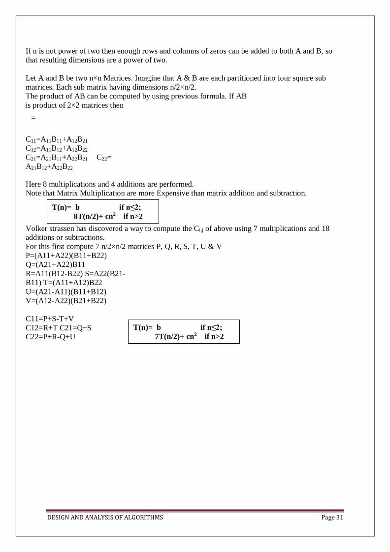
Strassen’s Matrix Multiplication:

Let A and B be two n×n Matrices. The product matrix C=AB is also a n×n matrix whose i, jth

element is formed by taking elements in the ith row of A and jth column of B and multiplying them

to get

C(i, j)=

Here 1≤ i & j ≤ n means i and j are in between 1 and n.

To compute C(i, j) using this formula, we need n multiplications.

The divide and conquer strategy suggests another way to compute the product of two n×n

matrices.

For Simplicity assume n is a power of 2 that is n=2k Here

k any nonnegative integer.


If n is not power of two then enough rows and columns of zeros can be added to both A and B, so

that resulting dimensions are a power of two.

Let A and B be two n×n Matrices. Imagine that A & B are each partitioned into four square sub

matrices. Each sub matrix having dimensions n/2×n/2.

The product of AB can be computed by using previous formula. If AB

is product of 2×2 matrices then

=

C11=A11B11+A12B21

C12=A11B12+A12B22

C21=A21B11+A22B21 C22=

A21B12+A22B22

Here 8 multiplications and 4 additions are performed.

Note that Matrix Multiplication are more Expensive than matrix addition and subtraction.

Volker strassen has discovered a way to compute the Ci,j of above using 7 multiplications and 18

additions or subtractions.

For this first compute 7 n/2×n/2 matrices P, Q, R, S, T, U & V

P=(A11+A22)(B11+B22)

Q=(A21+A22)B11

R=A11(B12-B22) S=A22(B21-

B11) T=(A11+A12)B22

U=(A21-A11)(B11+B12)

V=(A12-A22)(B21+B22)

C11=P+S-T+V

C12=R+T C21=Q+S

C22=P+R-Q+U

T(n)= b if n≤2;

7T(n/2)+ cn2 if n>2

T(n)= b if n≤2;

8T(n/2)+ cn2 if n>2


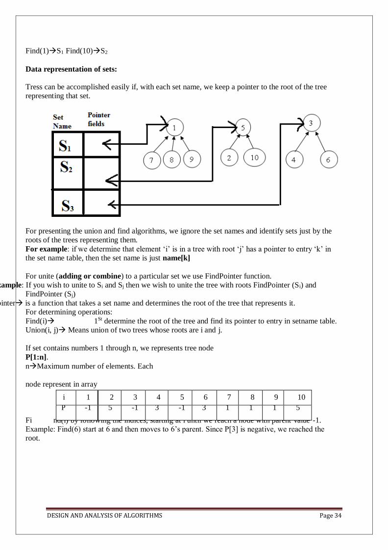
MODULE II:

Searching and Traversal Techniques: Efficient non - recursive binary tree traversal algorithm,

Disjoint set operations, union and find algorithms, Spanning trees, Graph traversals - Breadth

first search and Depth first search, AND / OR graphs, game trees, Connected Components, Bi -

connected components. Disjoint Sets- disjoint set operations,

union and find algorithms, spanning trees, connected components and biconnected

components.

Efficient non recursive tree traversal algorithms in-order: (left, root, right) 3,5,6,7,10,12,13

15, 16, 18, 20, 23

pre-order: (root, left, right) 15, 5, 3, 12, 10, 6, 7,

13, 16, 20, 18, 23

post-order: (left, right, root) 3, 7, 6,

10, 13, 12, 5,

18, 23,20,16, 65

Non recursive Inorder traversal algorithm

1. Start fiom the root. let's it is current.

2. Ifcurrent is not NULL. push the node on to stack.

3. Move to left child of current and go to step 2.

4. Ifcurrent is NULL, and stack is not empty, pop node from the stack.

5. Print the node value and change current to right child of current.

6. Go to step 2.

So we go on traversing all left node. as we visit the node. we will put that node into stack.remember

need to visit parent after the child and as We will encounter parent first when start from root. it's

case for LIFO :) and hence the stack). Once we reach NULL node. we will take the node at the top

of the stack. last node which we visited. Print it.

Check if there is right child to that node. If yes. move right child to stack and again start traversing

left child node and put them on to stack. Once we have traversed all node. our stack will be empty.

Non recursive postorder traversal algorithm Left

node. right node and last parent node.

1.1 Create an empty stack

Do Following while root is not NULL

a) Push root's right child and then root to stack.


S1 U S2

b) Set root as root's left child.

Pop an item from stack and set it as root.

a) If the popped item has a right child and the right child is at

top of stack, then remove the right child from stack, push the

root back and set root as root's right child.

Ia) Else print root's data and set root as NULL.

Repeat steps 2.1 and 2.2 while stack is not empty.

Disjoint Sets: If Si and Sj, i≠j are two sets, then there is no element that is in both Si and Sj..

For example: n=10 elements can be partitioned into three disjoint sets,

Tree representation of sets:

Disjoint set Operations:

Disjoint set Union

Find(i)

Disjoint set Union: Means Combination of two disjoint sets elements. Form above example S1 U S2

={1,7,8,9,5,2,10 }

For S1 U S2 tree representation, simply make one of the tree is a subtree of the other.

Find: Given element i, find the set containing i.

Form above example:

Find(4)S3

1 5 3

7 8 9 2 10 4 6 S1 S2 S3

S1= {1, 7, 8, 9}

S2= {2, 5, 10}

S3= {3, 4, 6}

1 1

7 8 9 5 5 7 8 9

2 10 2 10

S1 U S2 S2 U S1


nd(i) by following the indices, starting at i until we reach a node with parent value

Find(1)S1 Find(10)S2

Data representation of sets:

Tress can be accomplished easily if, with each set name, we keep a pointer to the root of the tree

representing that set.

For presenting the union and find algorithms, we ignore the set names and identify sets just by the

roots of the trees representing them.

For example: if we determine that element ‘i’ is in a tree with root ‘j’ has a pointer to entry ‘k’ in

the set name table, then the set name is just name[k]

For unite (adding or combine) to a particular set we use FindPointer function.

Example: If you wish to unite to Si and Sj then we wish to unite the tree with roots FindPointer (Si) and

FindPointer (Sj)

FindPointer is a function that takes a set name and determines the root of the tree that represents it.

For determining operations:

Find(i) 1St determine the root of the tree and find its pointer to entry in setname table.

Union(i, j) Means union of two trees whose roots are i and j.

If set contains numbers 1 through n, we represents tree node

P[1:n].

nMaximum number of elements. Each

node represent in array

Fi -1.

Example: Find(6) start at 6 and then moves to 6’s parent. Since P[3] is negative, we reached the

root.

i 1 2 3 4 5 6 7 8 9 10

P -1 5 -1 3 -1 3 1 1 1 5


Algorithm for finding Union(i, j): Algorithm for find(i)

Algorithm Simple union(i, j) {

P[i]:=j; // Accomplishes the union

}

Algorithm SimpleFind(i) {

While(P[i]≥0) do i:=P[i];

return i;

}

If n numbers of roots are there then the above algorithms are not useful for union and find. For

union of n trees Union(1,2), Union(2,3), Union(3,4),…..Union(n-1,n).

For Find i in n trees Find(1), Find(2),….Find(n).

Time taken for the union (simple union) is O(1) (constant).

For the n-1 unions O(n).

Time taken for the find for an element at level i of a tree is O(i).

For n finds O(n2).

To improve the performance of our union and find algorithms by avoiding the creation of

degenerate trees. For this we use a weighting rule for union(i, j)

Weighting rule for Union(i, j):

If the number of nodes in the tree with root ‘i’ is less than the tree with root ‘j’, then make ‘j’ the

parent of ‘i’; otherwise make ‘i’ the parent of ‘j’.


Algorithm for weightedUnion(i, j)

Algorithm WeightedUnion(i,j)

//Union sets with roots i and j, i≠j

// The weighting rule, p[i]= -count[i] and p[j]= -count[j].

{

temp := p[i]+p[j];

if (p[i]>p[j]) then

{ // i has fewer nodes.

P[i]:=j;

P[j]:=temp;

} else

{ // j has fewer or equal nodes.

P[j] := i;

P[i] := temp;

}

}

For implementing the weighting rule, we need to know how many nodes there are in

every tree.

For this we maintain a count field in the root of every tree. i

root node

count[i] number of nodes in the tree.

Time required for this above algorithm is O(1) + time for remaining unchanged is

determined by using Lemma.

Lemma:- Let T be a tree with m nodes created as a result of a sequence of unions each performed using

WeightedUnion. The height of T is no greater than

|log2 m|+1.


Collapsing rule: If ‘j’ is a node on the path from ‘i’ to its root and p[i]≠root[i], then set p[j] to root[i].

Algorithm for Collapsing find.

Algorithm CollapsingFind(i) //Find the root of the tree containing element i.

//collapsing rule to collapse all nodes form i to the root.

{

r;=i;

while(p[r]>0) do r := p[r]; //Find the root. While(i

≠ r) do // Collapse nodes from i to root r.

{

s:=p[i];

p[i]:=r;

i:=s;

}

return r; }

Collapsing find algorithm is used to perform find operation on the tree created by

WeightedUnion.

For example: Tree created by using WeightedUnion

Now process the following eight finds: Find(8), Find(8),… .................. Find(8)

If SimpleFind is used, each Find(8) requires going up three parent link fields for a total of 24 moves

to process all eight finds.


When CollapsingFind is uised the first Find(8) requires going up three links and then resetting

two links. Total 13 movies requies for process all eight finds.

Spanning Tree:- Let G=(V<E) be an undirected connected graph. A sub graph t=(V,E1) of G is a spanning tree of G iff

t is a tree.

Spanning Trees have many applications.

Example:-

It can be used to obtain an independent set of circuit equations for an electric network.

Any connected graph with n vertices must have at least n-1 edges and all connected graphs with n-1

edges are trees. If nodes of G represent cities and the edges represent possible communication links

connecting two cities, then the minimum number of links needed to connect the n cities is n-1.

There are two basic algorithms for finding minimum-cost spanning trees, and both are greedy

algorithms

Prim’s Algorithm

Kruskal’s Algorithm


Prim’s Algorithm: Start with any one node in the spanning tree, and repeatedly add the cheapest

edge, and the node it leads to, for which the node is not already in the spanning tree.

Kruskal’s Algorithm: Start with no nodes or edges in the spanning tree, and repeatedly add the

cheapest edge that does not create a cycle.

Connected Component:

Connected component of a graph can be obtained by using BFST (Breadth first search and

traversal) and DFST (Dept first search and traversal). It is also called the spanning tree.

BFST (Breadth first search and traversal):

In BFS we start at a vertex V mark it as reached (visited).

The vertex V is at this time said to be unexplored (not yet discovered).

A vertex is said to been explored (discovered) by visiting all vertices adjacent from it.

All unvisited vertices adjacent from V are visited next.

The first vertex on this list is the next to be explored.

Exploration continues until no unexplored vertex is left.

These operations can be performed by using Queue.

This is also called connected graph or spanning tree.

Spanning trees obtained using BFS then it called breadth first spanning trees.

Algorithm for BFS to convert undirected graph G to Connected component or spanning

tree.

Algorithm BFS(v) // a bfs of G is begin at vertex v

// for any node I, visited[i]=1 if I has already been visited.

// the graph G, and array visited[] are global

{


DFST(Dept first search and traversal).:

Dfs different from bfs

The exploration of a vertex v is suspended (stopped) as soon as a new vertex is reached.

In this the exploration of the new vertex (example v) begins; this new vertex has been explored, the

exploration of v continues.

Note: exploration start at the new vertex which is not visited in other vertex exploring and choose

nearest path for exploring next or adjacent vertex.

U:=v; // q is a queue of unexplored vertices.

Visited[v]:=1;

Repeat{

For all vertices w adjacent from U do

If (visited[w]=0) then

{

Add w to q; // w is unexplored

Visited[w]:=1;

}

If q is empty then return; // No unexplored vertex.

Delete U from q; //Get 1st unexplored vertex.

} Until(false)

}

Maximum Time complexity and space complexity of G(n,e), nodes are in adjacency list.

T(n, e)=θ(n+e)

S(n, e)=θ(n)

If nodes are in adjacency matrix then

T(n, e)=θ(n2)

S(n, e)=θ(n)


Algorithm for DFS to convert undirected graph G to Connected component or spanning

tree.

Algorithm dFS(v) // a Dfs of G is begin at vertex v

// initially an array visited[] is set to zero.

//this algorithm visits all vertices reachable from v.

// the graph G, and array visited[] are global

{

Visited[v]:=1;

For each vertex w adjacent from v do

{

If (visited[w]=0) then DFS(w);

{

Add w to q; // w is unexplored

Visited[w]:=1;

}

}

Maximum Time complexity and space complexity of G(n,e), nodes are in adjacency list.

T(n, e)=θ(n+e)

S(n, e)=θ(n)

If nodes are in adjacency matrix then

T(n, e)=θ(n2) S(n, e)=θ(n)

Bi-connected Components:


A graph G is biconnected, iff (if and only if) it contains no articulation point (joint or junction).

A vertex v in a connected graph G is an articulation point, if and only if (iff) the deletion of vertex v

together with all edges incident to v disconnects the graph into two or more none empty

components.

The presence of articulation points in a connected graph can be an undesirable(un wanted) feature in

many cases.

For example

if G1Communication network with Vertex

communication stations. Edges

Communication lines.

Then the failure of a communication station I that is an articulation point, then we loss the

communication in between other stations. F

Form graph G1

(Here 2 is articulation point)

If the graph is bi-connected graph (means no articulation point) then if any station i fails, we

can still communicate between every two stations not including station i.


From Graph Gb

There is an efficient algorithm to test whether a connected graph is biconnected. If the case of graphs

that are not biconnected, this algorithm will identify all the articulation points.

Once it has been determined that a connected graph G is not biconnected, it may be desirable

(suitable) to determine a set of edges whose inclusion makes the graph biconnected.


MODULE III:

Greedy method: General method, applications - Job sequencing with deadlines, 0/1 knapsack

problem, Minimum cost spanning trees, Single source shortest path problem. Dynamic

Programming: General method, applications-Matrix chain multiplication, Optimal binary search

trees, 0/1 knapsack problem, All pairs shortest path problem, Travelling sales person problem,

Reliability design.

Greedy Method:

The greedy method is perhaps (maybe or possible) the most straight forward design

technique, used to determine a feasible solution that may or may not be optimal.

Feasible solution:- Most problems have n inputs and its solution contains a subset of inputs that

satisfies a given constraint(condition). Any subset that satisfies the constraint is called feasible

solution.

Optimal solution: To find a feasible solution that either maximizes or minimizes a given

objective function. A feasible solution that does this is called optimal solution.

The greedy method suggests that an algorithm works in stages, considering one input at a time. At

each stage, a decision is made regarding whether a particular input is in an optimal solution.

Greedy algorithms neither postpone nor revise the decisions (ie., no back tracking). Example:

Kruskal’s minimal spanning tree. Select an edge from a sorted list, check, decide, and never visit it

again.

Application of Greedy Method:

Job sequencing with deadline

0/1 knapsack problem

Minimum cost spanning trees

Single source shortest path problem.

Algorithm for Greedy method

Algorithm Greedy(a,n) //a[1:n] contains the n inputs.

{

Solution :=0;

For i=1 to n do

{

X:=select(a);

If Feasible(solution, x) then

Solution :=Union(solution,x);

}

Return solution; }

Selection Function, that selects an input from a[] and removes it. The selected input’s value

is assigned to x.

Feasible Boolean-valued function that determines whether x can be included into the

solution vector.

Union function that combines x with solution and updates the objective function.


Knapsack problem

The knapsack problem or rucksack (bag) problem is a problem in combinatorial optimization: Given a set of items,

each with a mass and a value, determine the number of each item to include in a collection so that the total weight is less

than or equal to a given limit and the total value is as large as possible

There are two versions of the problems

1. 0/1 knapsack problem

2. Fractional Knapsack problem

a. Bounded Knapsack problem.

b. Unbounded Knapsack problem.

Solutions to knapsack problems

Brute-force approach:-Solve the problem with a straight farward algorithm

Greedy Algorithm:- Keep taking most valuable items until maximum weight is reached or taking

the largest value of eac item by calculating vi=valuei/Sizei

Dynamic Programming:- Solve each sub problem once and store their solutions in an array.

http://en.wikipedia.org/wiki/Combinatorial_optimization


0/1 knapsack problem:

Let there be items, to where has a value and weight . The maximum weight that

we can carry in the bag is W. It is common to assume that all values and weights are nonnegative. To

simplify the representation, we also assume that the items are listed in increasing order of weight.

Maximize subject to

Maximize the sum of the values of the items in the knapsack so that the sum of the weights must be less than the

knapsack's capacity.

Greedy algorithm for knapsack

Algorithm GreedyKnapsack(m,n) // p[i:n] and [1:n] contain the profits and weights respectively

// if the n-objects ordered such that p[i]/w[i]>=p[i+1]/w[i+1], m size of knapsack and

x[1:n] the solution vector

{

For i:=1 to n do x[i]:=0.0

U:=m;

For i:=1 to n do

{

if(w[i]>U) then break;

x[i]:=1.0;

U:=U-w[i];

}

If(i<=n) then x[i]:=U/w[i];

}

Ex: - Consider 3 objects whose profits and weights are defined as (P1,

P2, P3) = ( 25, 24, 15 ) W1, W2, W3) = ( 18, 15, 10 ) n=3number of objects m=20Bag capacity

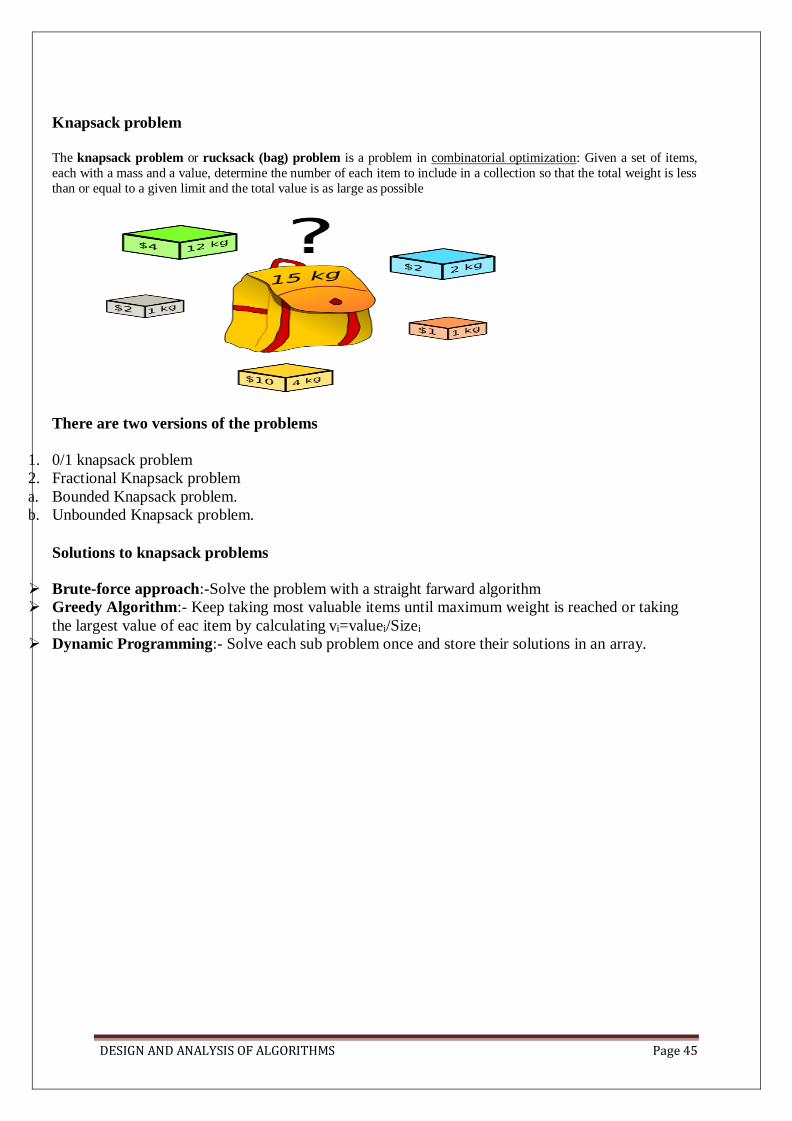
Consider a knapsack of capacity 20. Determine the optimum strategy for placing the objects in to the knapsack. The problem can be solved by the greedy approach where in the inputs are arranged according to selection process (greedy strategy) and solve the problem in stages. The various greedy strategies for the problem could be as follows.

(x1, x2, x3) ∑ xiwi ∑ xipi

(1, 2/15, 0) 2 18x1+ x15 = 20 15

2 25x1+ x 24 = 28.2 15

(0, 2/3, 1) 2 x15+10x1= 20 3

2 x 24 +15x1 = 31

3


(0, 1, ½ ) 1x15+

1 x10 = 20

2 1x24+

1 x15 = 31.5

2

(½, ⅓, ¼ ) ½ x 18+⅓ x15+ ¼ x10 = 16. 5 ½ x 25+⅓ x24+ ¼ x15 = 12.5+8+3.75 = 24.25

Analysis: - If we do not consider the time considered for sorting the inputs then all of the three greedy strategies complexity will be O(n).

Job Sequence with Deadline:

There is set of n-jobs. For any job i, is a integer deadling di≥0 and profit Pi>0, the profit Pi is earned

iff the job completed by its deadline.

To complete a job one had to process the job on a machine for one unit of time. Only one machine

is available for processing jobs.

A feasible solution for this problem is a subset J of jobs such that each job in this subset can be

completed by its deadline.

The value of a feasible solution J is the sum of the profits of the jobs in J, i.e., ∑i∈jPi

An optimal solution is a feasible solution with maximum value.

The problem involves identification of a subset of jobs which can be completed by its deadline. Therefore the problem suites the subset methodology and can be solved by the greedy method.


Ex: - Obtain the optimal sequence for the following jobs.

j1 j2 j3 j4

(P1, P2, P3, P4) = (100, 10, 15, 27)

(d1, d2, d3, d4) = (2, 1, 2, 1)

n =4

Feasible

solution

Processing sequence Value

j1 j2

(1, 2) (2,1) 100+10=110

(1,3) (1,3) or (3,1) 100+15=115

(1,4) (4,1) 100+27=127

(2,3) (2,3) 10+15=25

(3,4) (4,3) 15+27=42

(1) (1) 100

(2) (2) 10

(3) (3) 15

(4) (4) 27

In the example solution ‘3’ is the optimal. In this solution only jobs 1&4 are processed and the

value is 127. These jobs must be processed in the order j4 followed by j1. the process of job 4 begins

at time 0 and ends at time 1. And the processing of job 1 begins at time 1 and ends at time2.

Therefore both the jobs are completed within their deadlines. The optimization measure for

determining the next job to be selected in to the solution is according to the profit. The next job to

include is that which increases ∑pi the most, subject to the constraint that the resulting “j” is the

feasible solution. Therefore the greedy strategy is to consider the jobs in decreasing order of profits.


The greedy algorithm is used to obtain an optimal solution.

We must formulate an optimization measure to determine how the next job is chosen.

Note: The size of sub set j must be less than equal to maximum deadline in given list.

Single Source Shortest Paths:

Graphs can be used to represent the highway structure of a state or country with vertices

representing cities and edges representing sections of highway.

The edges have assigned weights which may be either the distance between the 2 cities connected by

the edge or the average time to drive along that section of highway.

For example if A motorist wishing to drive from city A to B then we must answer the following

questions

o Is there a path from A to B

o If there is more than one path from A to B which is the shortest path The length of a path is defined to be the sum of the weights of the edges on that path.

Given a directed graph G(V,E) with weight edge w(u,v). e have to find a shortest path from source

vertex S∈v to every other vertex v1∈ v-s.

algorithm js(d, j, n)

//d dead line, jsubset of jobs ,n total number of jobs

// d[i]≥1 1 ≤ i ≤ n are the dead lines,

// the jobs are ordered such that p[1]≥p[2]≥---≥p[n]

//j[i] is the ith job in the optimal solution 1 ≤ i ≤ k, k subset range

{

d[0]=j[0]=0;

j[1]=1;

k=1;

for i=2 to n do{

r=k;

while((d[j[r]]>d[i]) and [d[j[r]]≠r)) do

r=r-1;

if((d[j[r]]≤d[i]) and (d[i]> r)) then

{

for q:=k to (r+1) setp-1 do j[q+1]= j[q];

j[r+1]=i;

k=k+1;

}

}

return k;

}


To find SSSP for directed graphs G(V,E) there are two different algorithms.

Bellman-Ford Algorithm

Dijkstra’s algorithm

Bellman-Ford Algorithm:- allow –ve weight edges in input graph. This algorithm

either finds a shortest path form source vertex S∈V to other vertex v∈V or detect a – ve weight cycles in G, hence no solution. If there is no negative weight cycles are

reachable form source vertex S∈V to every other vertex v∈V

Dijkstra’s algorithm:- allows only +ve weight edges in the input graph and finds a shortest path from

source vertex S∈V to every other vertex v∈V.

Consider the above directed graph, if node 1 is the source vertex, then shortest path from 1 to 2 is

1,4,5,2. The length is 10+15+20=45.

To formulate a greedy based algorithm to generate the shortest paths, we must conceive of a

multistage solution to the problem and also of an optimization measure.

This is possible by building the shortest paths one by one.

As an optimization measure we can use the sum of the lengths of all paths so far generated.

If we have already constructed ‘i’ shortest paths, then using this optimization measure, the next path

to be constructed should be the next shortest minimum length path.

The greedy way to generate the shortest paths from Vo to the remaining vertices is to generate these

paths in non-decreasing order of path length.

For this 1st, a shortest path of the nearest vertex is generated. Then a shortest path to the 2nd nearest

vertex is generated and so on.


Algorithm for finding Shortest Path

Algorithm ShortestPath(v, cost, dist, n)

//dist[j], 1≤j≤n, is set to the length of the shortest path from vertex v to vertex j in graph g with

n-vertices.

// dist[v] is zero

{

for i=1 to n do{

s[i]=false;

dist[i]=cost[v,i];

}

s[v]=true;

dist[v]:=0.0; // put v in s

for num=2 to n do{

// determine n-1 paths from v

choose u form among those vertices not in s such that dist[u] is minimum.

s[u]=true; // put u in s

for (each w adjacent to u with s[w]=false) do

if(dist[w]>(dist[u]+cost[u, w])) then

dist[w]=dist[u]+cost[u, w];

} }

Minimum Cost Spanning Tree:

SPANNING TREE: - A Sub graph ‘n’ of o graph ‘G’ is called as a spanning tree if

(i) It includes all the vertices of ‘G’

(ii) It is a tree

Minimum cost spanning tree: For a given graph ‘G’ there can be more than one spanning tree. If

weights are assigned to the edges of ‘G’ then the spanning tree which has the minimum cost of

edges is called as minimal spanning tree.

The greedy method suggests that a minimum cost spanning tree can be obtained by contacting the

tree edge by edge. The next edge to be included in the tree is the edge that results in a minimum

increase in the some of the costs of the edges included so far.

There are two basic algorithms for finding minimum-cost spanning trees, and both are greedy

algorithms

Prim’s Algorithm

Kruskal’s Algorithm

Prim’s Algorithm: Start with any one node in the spanning tree, and repeatedly add the cheapest

edge, and the node it leads to, for which the node is not already in the spanning tree.


PRIM’S ALGORITHM: - i) Select an edge with minimum cost and include in to the spanning tree. ii) Among all the edges which are adjacent with the selected edge, select the one with minimum cost. iii) Repeat step 2 until ‘n’ vertices and (n-1) edges are been included. And the sub graph obtained does

not contain any cycles. Notes: - At every state a decision is made about an edge of minimum cost to be included into the spanning tree. From the edges which are adjacent to the last edge included in the spanning tree i.e. at every stage the sub-graph obtained is a tree.


Prim's minimum spanning tree algorithm

Algorithm Prim (E, cost, n,t) // E is the set of edges in G. Cost (1:n, 1:n) is the // Cost adjacency matrix of an n vertex graph such that // Cost (i,j) is either a positive real no. or ∞ if no edge (i,j) exists.

//A minimum spanning tree is computed and //Stored in the array T(1:n-1, 2). //(t (i, 1), + t(i,2)) is an edge in the minimum cost spanning tree. The final cost is returned { Let (k, l) be an edge with min cost in E Min cost: = Cost (x,l); T(1,1):= k; + (1,2):= l; for i:= 1 to n do//initialize near if (cost (i,l)<cost (i,k) then n east (i): l; else near (i): = k; near (k): = near (l): = 0; for i: = 2 to n-1 do {//find n-2 additional edges for t

let j be an index such that near (i) 0 & cost (j, near (i)) is minimum; t (i,1): = j + (i,2): = near (j); min cost: = Min cost + cost (j, near (j)); near (j): = 0;

for k:=1 to n do // update near ()

if ((near (k) 0) and (cost {k, near (k)) > cost (k,j))) then near Z(k): = ji } return mincost; }

The algorithm takes four arguments E: set of edges, cost is nxn adjacency matrix cost of (i,j)= +ve integer, if an edge exists between i&j otherwise infinity. ‘n’ is no/: of vertices. ‘t’ is a (n-1):2matrix which consists of the edges of spanning tree. E = { (1,2), (1,6), (2,3), (3,4), (4,5), (4,7), (5,6), (5,7), (2,7) } n = {1,2,3,4,5,6,7)


i) The algorithm will start with a tree that includes only minimum cost edge of

G. Then edges are added to this tree one by one. ii) The next edge (i,j) to be added is such that i is a vertex which is already included in the treed and j

is a vertex not yet included in the tree and cost of i,j is minimum among all edges adjacent to ‘i’. iii) With each vertex ‘j’ next yet included in the tree, we assign a value near ‘j’. The value near ‘j’

represents a vertex in the tree such that cost (j, near (j)) is minimum among all choices for near (j)

iv) We define near (j):= 0 for all the vertices ‘j’ that are already in the tree.

v) The next edge to include is defined by the vertex ‘j’ such that (near (j)) 0 and cost of (j, near (j)) is minimum.

Analysis: - The time required by the prince algorithm is directly proportional to the no/: of vertices. If a graph ‘G’ has ‘n’ vertices then the time required by prim’s algorithm is 0(n2)


Kruskal’s Algorithm: Start with no nodes or edges in the spanning tree, and repeatedly add the

cheapest edge that does not create a cycle. In Kruskals algorithm for determining the spanning tree we arrange the edges in the increasing order of cost.

i) All the edges are considered one by one in that order and deleted from the graph and are included in to the spanning tree.

ii) At every stage an edge is included; the sub-graph at a stage need not be a tree. Infect it is a forest. iii) At the end if we include ‘n’ vertices and n-1 edges without forming cycles then we get a single

connected component without any cycles i.e. a tree with minimum cost. At every stage, as we include an edge in to the spanning tree, we get disconnected trees represented by various sets. While including an edge in to the spanning tree we need to check it does not form cycle. Inclusion of an edge (i,j) will form a cycle if i,j both are in same set. Otherwise the edge can be included into the spanning tree.

Kruskal minimum spanning tree algorithm Algorithm Kruskal (E, cost, n,t) //E is the set of edges in G. ‘G’ has ‘n’ vertices

//Cost {u,v} is the cost of edge (u,v) t is the set

//of edges in the minimum cost spanning tree //The final cost is returned { construct a heap out of the edge costs using heapify;

for i:= 1 to n do parent (i):= -1 // place in different sets

//each vertex is in different set {1} {1} {3}

i: = 0; min cost: = 0.0;

While (i<n-1) and (heap not empty))do

{ Delete a minimum cost edge (u,v) from the heaps; and reheapify using adjust; j:=

find (u); k:=find (v);

if (jk) then

{ i: = 1+1; + (i,1)=u; + (i, 2)=v;

mincost: = mincost+cost(u,v);

Union (j,k);

} }

if (in-1) then write (“No spanning tree”); else

return mincost;

}

Consider the above graph of , Using Kruskal's method the edges of this graph are considered for

inclusion in the minimum cost spanning tree in the order (1, 2), (3, 6), (4, 6), (2, 6), (1, 4),

(3, 5), (2, 5), (1, 5), (2, 3), and (5, 6). This corresponds to the cost sequence 10, 15, 20, 25, 30, 35,

40, 45, 50, 55. The first four edges are included in T. The next edge to be considered is (I, 4). This

edge connects two vertices already connected in T and so it is rejected. Next, the edge (3, 5) is

selected and that completes the spanning tree.


Analysis: - If the no/: of edges in the graph is given by /E/ then the time for Kruskals algorithm is given by 0 (|E| log |E|).


Dynamic Programming

Dynamic programming is a name, coined by Richard Bellman in 1955. Dynamic programming, as

greedy method, is a powerful algorithm design technique that can be used when the solution to the

problem may be viewed as the result of a sequence of decisions. In the greedy method we make

irrevocable decisions one at a time, using a greedy criterion. However, in dynamic programming we

examine the decision sequence to see whether an optimal decision sequence contains optimal

decision subsequence.

When optimal decision sequences contain optimal decision subsequences, we can establish

recurrence equations, called dynamic-programming recurrence equations, that enable us to solve the

problem in an efficient way.

Dynamic programming is based on the principle of optimality (also coined by Bellman). The

principle of optimality states that no matter whatever the initial state and initial decision are, the

remaining decision sequence must constitute an optimal decision sequence with regard to the state

resulting from the first decision. The principle implies that an optimal decision sequence is

comprised of optimal decision subsequences. Since the principle of optimality may not hold for some

formulations of some problems, it is necessary to verify that it does hold for the problem being

solved. Dynamic programming cannot be applied when this principle does not hold.

The steps in a dynamic programming solution are:

Verify that the principle of optimality holds

Set up the dynamic-programming recurrence equations

Solve the dynamic-programming recurrence equations for the value of the optimal solution.

Perform a trace back step in which the solution itself is constructed.

5.1 MULTI STAGE GRAPHS

A multistage graph G = (V, E) is a directed graph in which the vertices are partitioned into k

> 2 disjoint sets Vi, 1 < i < k. In addition, if <u, v> is an edge in E, then u E Vi and v E Vi+1 for

some i, 1 < i < k.

Let the vertex ‘s’ is the source, and ‘t’ the sink. Let c (i, j) be the cost of edge <i, j>. The cost of a

path from ‘s’ to ‘t’ is the sum of the costs of the edges on the path. The multistage graph problem is to

find a minimum cost path from ‘s’ to ‘t’. Each set Vi defines a stage in the graph. Because of the

constraints on E, every path from ‘s’ to ‘t’ starts in stage 1, goes to stage 2, then to stage 3, then to

stage 4, and so on, and eventually terminates in stage k.

A dynamic programming formulation for a k-stage graph problem is obtained by first noticing that

every s to t path is the result of a sequence of k – 2 decisions. The ith


decision involves determining which vertex in vi+1, 1 < i < k - 2, is to be on the path. Let c (i, j) be

the cost of the path from source to destination. Then using the forward approach, we obtain:

cost (i, j) = min {c (j, l) + cost (i + 1, l)}

l c Vi + 1 <j, l> c E

ALGORITHM:

Algorithm Fgraph (G, k, n, p)

// The input is a k-stage graph G = (V, E) with n vertices // indexed in

order or stages. E is a set of edges and c [i, j] // is the cost of (i, j). p [1

: k] is a minimum cost path.

{

cost [n] := 0.0;

for j:= n - 1 to 1 step – 1 do

{ // compute cost [j]

let r be a vertex such that (j, r) is an edge of G and c [j, r] + cost [r] is

minimum; cost [j] := c [j, r] + cost [r];

d [j] := r:

}

p [1] := 1; p [k] := n; // Find a minimum cost path.

for j := 2 to k - 1 do p [j] := d [p [j - 1]];}

The multistage graph problem can also be solved using the backward approach. Let bp(i,

j) be a minimum cost path from vertex s to j vertex in Vi. Let Bcost(i, j) be the cost of bp(i, j).

From the backward approach we obtain:

Bcost (i, j) = min { Bcost (i –1, l) + c (l, j)} l e Vi - 1 <l, j> e E

Algorithm Bgraph (G, k, n, p)

// Same function as Fgraph {

Bcost [1] := 0.0; for j := 2 to n do { / / C o m p u t e

B c o s t [ j ] .

Let r be such that (r, j) is an edge of G and Bcost [r] + c [r,

j] is minimum; Bcost [j] := Bcost [r] + c [r, j];

D [j] := r;

} //find a minimum cost path

p [1] := 1; p [k] := n;

for j:= k - 1 to 2 do p [j] := d [p [j + 1]];

}

Complexity Analysis:


The complexity analysis of the algorithm is fairly straightforward. Here, if G has ~E~ edges, then

the time for the first for loop is CJ ( V~ +~E ).

EXAMPLE 1:

Find the minimum cost path from s to t in the multistage graph of five stages shown below. Do this first

using forward approach and then using backward approach.

FORWARD APPROACH:

We use the following equation to find the minimum cost path from s to t: cost (i,

j) = min {c (j, l) + cost (i + 1, l)} l c Vi + 1

<j, l> c E cost (1, 1) = min {c (1, 2) + cost (2, 2), c (1, 3) + cost (2, 3), c (1, 4) + cost (2, 4), c (1, 5) +

cost (2, 5)}

= min {9 + cost (2, 2), 7 + cost (2, 3), 3 + cost (2, 4), 2 + cost (2, 5)}

Now first starting with,

cost (2, 2) = min{c (2, 6) + cost (3, 6), c (2, 7) + cost (3, 7), c (2, 8) + cost (3, 8)} = min {4 +

cost (3, 6), 2 + cost (3, 7), 1 + cost (3, 8)}

cost (3, 6) = min {c (6, 9) + cost (4, 9), c (6, 10) + cost (4, 10)}

= min {6 + cost (4, 9), 5 + cost (4, 10)}

cost (4, 9) = min {c (9, 12) + cost (5, 12)} = min {4 + 0) = 4 cost (4,

10) = min {c (10, 12) + cost (5, 12)} = 2

Therefore, cost (3, 6) = min {6 + 4, 5 + 2} = 7

t

cost (3, 7) = min {c (7, 9) + cost (4, 9) , c (7, 10) + cost (4, 10)}

= min {4 + cost (4, 9), 3 + cost (4, 10)}

7 1 0 3

2 4 11 5

5 11 8 1 1

6

5 8

2 4 6 2 6 9

9 1 2 5 4

7

3

7

4 2

1 2

s 1 3


cost (4, 9) = min {c (9, 12) + cost (5, 12)} = min {4 + 0} = 4 Cost (4,

10) = The path is 1 2 7 10 12

min

{c (10,

or

1 3 6 10 12

2) + cost (5, 12)} = min {2 + 0} = 2 Therefore, cost (3, 7) = min {4 + 4, 3

+ 2} = min {8, 5} = 5


= min {5 + cost (4, 10), 6 + cost (4 + 11)}

cost (4, 11) = min {c (11, 12) + cost (5, 12)} = 5

Therefore, cost (3, 8) = min {5 + 2, 6 + 5} = min {7, 11} = 7

Therefore, cost (2, 2) = min {4 + 7, 2 + 5, 1 + 7} = min {11, 7, 8} = 7

Therefore, cost (2, 3) = min {c (3, 6) + cost (3, 6), c (3, 7) + cost (3, 7)}

= min {2 + cost (3, 6), 7 + cost (3, 7)}

= min {2 + 7, 7 + 5} = min {9, 12} = 9

cost (2, 4) = min {c (4, 8) + cost (3, 8)} = min {11 + 7} = 18 cost (2, 5) =

min {c (5, 7) + cost (3, 7), c (5, 8) + cost (3, 8)} = min {11 + 5, 8 +

7} = min {16, 15} = 15

Therefore, cost (1, 1) = min {9 + 7, 7 + 9, 3 + 18, 2 + 15} = min

{16, 16, 21, 17} = 16

The minimum cost path is 16. BACKWARD APPROACH:

We use the following equation to find the minimum cost path from t to s: Bcost (i, J) = min

{Bcost (i – 1, l) + c (l, J)}

l c vi – 1 <l, j> c E

Bcost (5, 12) = min {Bcost (4, 9) + c (9, 12), Bcost (4, 10) + c (10, 12),

Bcost (4, 11) + c (11, 12)}

= min {Bcost (4, 9) + 4, Bcost (4, 10) + 2, Bcost (4, 11) + 5}

Bcost (4, 9) = min {Bcost (3, 6) + c (6, 9), Bcost (3, 7) + c (7, 9)}

= min {Bcost (3, 6) + 6, Bcost (3, 7) + 4}


= min {Bcost (2, 2) + 4, Bcost (2, 3) + 2}


Bcost (2, 2) = min {Bcost (1, 1) + c (1, 2)} = min {0 + 9} = 9 Bcost (2, 3) = min

{Bcost (1, 1) + c (1, 3)} = min {0 + 7} = 7 Bcost (3, 6) = min {9 + 4, 7 + 2} =

min {13, 9} = 9

Bcost (3, 7) = min {Bcost (2, 2) + c (2, 7), Bcost (2, 3) + c (3, 7), Bcost (2, 5) + c (5,

7)}

Bcost (2, 5) = min {Bcost (1, 1) + c (1, 5)} = 2

Bcost (3, 7) = min {9 + 2, 7 + 7, 2 + 11} = min {11, 14, 13} = 11 Bcost (4, 9) = min {9

+ 6, 11 + 4} = min {15, 15} = 15


Bcost (3, 8) + c (8, 10)}


Bcost (2, 5) + c (5, 8)}

Bcost (2, 4) = min {Bcost (1, 1) + c (1, 4)} = 3

Bcost (3, 8) = min {9 + 1, 3 + 11, 2 + 8} = min {10, 14, 10} = 10 Bcost (4, 10) = min {9

+ 5, 11 + 3, 10 + 5} = min {14, 14, 15) = 14

Bcost (4, 11) = min {Bcost (3, 8) + c (8, 11)} = min {Bcost (3, 8) + 6} = min {10 + 6} =

16


Bcost (5, 12) = min {15 + 4, 14 + 2, 16 + 5} = min {19, 16, 21} = 16. EXAMPLE

2:

Find the minimum cost path from s to t in the multistage graph of five stages shown below. Do this first

using forward approach and then using backward approach.

3 4 1

5 2

6 4 7

7

3 6

s 1 5 2 9 t

8 3

6

8 6 2

2 5 3

SOLUTION: FORWARD

APPROACH:

cost (i, J) = min {c (j, l) + cost (i + 1, l)}

l c Vi + 1

<J, l> EE


= min {5 + cost (2, 2), 2 + cost (2, 3)}


= min {3+ cost (3, 4), 3 + cost (3, 6)}


= min {(1 + cost (4, 7), 4 + cost (4, 8)}

cost (4, 7) = min {c (7, 9) + cost (5, 9)} = min {7 + 0) = 7 cost (4, 8)

= min {c (8, 9) + cost (5, 9)} = 3

Therefore, cost (3, 4) = min {8, 7} = 7


= min {6 + cost (4, 7), 2 + cost (4, 8)} = min {6 + 7, 2 + 3} = 5

Therefore, cost (2, 2) = min {10, 8} = 8

cost (2, 3) = min {c (3, 4) + cost (3, 4), c (3, 5) + cost (3, 5), c (3, 6) + cost (3,6)}

cost (3, 5) = min {c (5, 7) + cost (4, 7), c (5, 8) + cost (4, 8)}= min {6 + 7, 2 + 3} = 5

104


Therefore, cost (2, 3) = min {13, 10, 13} = 10

cost (1, 1) = min {5 + 8, 2 + 10} = min {13, 12} = 12

BACKWARD APPROACH:

Bcost (i, J) = min {Bcost (i – 1, l) = c (l, J)} l E vi – 1

<l ,j>E E


= min {Bcost (4, 7) + 7, Bcost (4, 8) + 3}


Bcost (3, 6) + c (6, 7)}

= min {Bcost (3, 4) + 1, Bcost (3, 5) + 6, Bcost (3, 6) + 6}


= min {Bcost (2, 2) + 3, Bcost (2, 3) + 6}

Bcost (2, 2) = min {Bcost (1, 1) + c (1, 2)} = min {0 + 5} = 5

Bcost (2, 3) = min (Bcost (1, 1) + c (1, 3)} = min {0 + 2} = 2

Therefore, Bcost (3, 4) = min {5 + 3, 2 + 6} = min {8, 8} = 8

Bcost (3, 5) = min {Bcost (2, 3) + c (3, 5)} = min {2 + 5} = 7

Bcost (3, 6) = min {Bcost (2, 2) + c (2, 6), Bcost (2, 3) + c (3, 6)} = min

{5 + 5, 2 + 8} = 10

Therefore, Bcost (4, 7) = min {8 + 1, 7 + 6, 10 + 6} = 9

Bcost (4, 8) = min {Bcost (3, 4) + c (4, 8), Bcost (3, 5) + c (5, 8), Bcost

(3, 6) + c (6, 8)}

= min {8 + 4, 7 + 2, 10 + 2} = 9

Therefore, Bcost (5, 9) = min {9 + 7, 9 + 3} = 12 All

pairs shortest paths

In the all pairs shortest path problem, we are to find a shortest path between every pair of vertices

in a directed graph G. That is, for every pair of vertices (i, j), we are to find a shortest path from i

to j as well as one from j to i. These two paths are the same when G is undirected.

When no edge has a negative length, the all-pairs shortest path problem may be solved by using

Dijkstra’s greedy single source algorithm n times, once with each of the n vertices as the source

vertex.

The all pairs shortest path problem is to determine a matrix A such that A (i, j) is the length of a

shortest path from i to j. The matrix A can be obtained by solving n single-source

105


problems using the algorithm shortest Paths. Since each application of this procedure requires

O (n2) time, the matrix A can be obtained in O (n3) time.

The dynamic programming solution, called Floyd’s algorithm, runs in O (n3) time. Floyd’s

algorithm works even when the graph has negative length edges (provided there are no negative

length cycles).

The shortest i to j path in G, i ≠ j originates at vertex i and goes through some intermediate

vertices (possibly none) and terminates at vertex j. If k is an intermediate vertex on this

shortest path, then the subpaths from i to k and from k to j must be shortest paths from i to k and

k to j, respectively. Otherwise, the i to j path is not of minimum length. So, the principle of

optimality holds. Let Ak (i, j) represent the length of a shortest path from i to j going through no

vertex of index greater than k, we obtain:

Ak (i, j) = {min {min {Ak-1 (i, k) + Ak-1 (k, j)}, c (i, j)} 1<k<n

Algorithm All Paths (Cost, A, n)

// cost [1:n, 1:n] is the cost adjacency matrix of a graph which

// n vertices; A [I, j] is the cost of a shortest path from vertex

// i to vertex j. cost [i, i] = 0.0, for 1 < i < n. { for i := 1 to n do for j:= 1 to n do

A [i, j] := cost [i, j]; // copy cost into A. for k := 1 to n do

for i := 1 to n do for j := 1 to n do A [i, j] := min (A [i, j], A [i, k] + A [k, j]);

}

Complexity Analysis: A Dynamic programming algorithm based on this recurrence involves in

calculating n+1 matrices, each of size n x n. Therefore, the algorithm has a complexity of O (n3).

Example 1:

Given a weighted digraph G = (V, E) with weight. Determine the length of the shortest path

between all pairs of vertices in G. Here we assume that there are no cycles with zero or negative

cost.

~r0 Cost adjacency matrix (A0) = ~6

~L3

4 0

~

11

2~~

0~]

6

1 2 4

3 1 1 2

3


General formula: min {Ak-1 (i, k) + Ak-1 (k, j)}, c (i, j)} 1<k<n

Solve the problem for different values of k = 1, 2 and 3 Step 1:

Solving the equation for, k = 1;

A1 (1, 1) = min {(Ao (1, 1) + Ao (1, 1)), c (1, 1)} = min {0 + 0, 0} = 0 A1 (1,

2) = min {(Ao (1, 1) + Ao (1, 2)), c (1, 2)} = min {(0 + 4), 4} = 4

A1 (1, 3) = min {(Ao (1, 1) + Ao (1, 3)), c (1, 3)} = min {(0 + 11), 11} = 11 A1 (2,

1) = min {(Ao (2, 1) + Ao (1, 1)), c (2, 1)} = min {(6 + 0), 6} = 6

A1 (2, 2) = min {(Ao (2, 1) + Ao (1, 2)), c (2, 2)} = min {(6 + 4), 0)} = 0 A1 (2,

3) = min {(Ao (2, 1) + Ao (1, 3)), c (2, 3)} = min {(6 + 11), 2} = 2 A1 (3, 1) =

min {(Ao (3, 1) + Ao (1, 1)), c (3, 1)} = min {(3 + 0), 3} = 3 A1 (3, 2) = min

{(Ao (3, 1) + Ao (1, 2)), c (3, 2)} = min {(3 + 4), oc} = 7 A1 (3, 3) = min {(Ao

(3, 1) + Ao (1, 3)), c (3, 3)} = min {(3 + 11), 0} = 0

A(1) =

Step 2: Solving the equation for, K = 2;

A2 (1,

A2 (1,

A2 (1,

A2 (2,

A2 (2,

A2 (2,

A2 (3,

A2 (3,

A2 (3,

A(2) =

~0 ~ ~6 ~L3

4

0

7

11 ~

2~ 0~U

1) = min {(A1 (1, 2)

2) = min {(A1 (1, 2)

3) = min {(A1 (1, 2)

+ A1 (2, 1), c (1, 1)} = min {(4 + 6), 0} + A1

(2, 2), c (1, 2)} = min {(4 + 0), 4} + A1 (2,

3), c (1, 3)} = min {(4 + 2), 11}

= 0

= 4

= 6

1) = min {(A (2, 2) + A (2, 1), c (2, 1)} = min {(0 + 6), 6} = 6

2) = min {(A (2, 2) + A (2, 2), c (2, 2)} = min {(0 + 0), 0} = 0

3) = min {(A (2, 2) + A (2, 3), c (2, 3)} = min {(0 + 2), 2} = 2

1) = min {(A (3, 2) + A (2, 1), c (3, 1)} = min {(7 + 6), 3} = 3

2) = min {(A (3, 2) + A (2, 2), c (3, 2)} = min {(7 + 0), 7} = 7

3) = min {(A (3, 2) + A (2, 3), c (3, 3)} = min {(7 + 2), 0} = 0

~0 ~ ~6 ~L3

4

0

7

6 1

2~ ~

0~~


Step 3: Solving the equation for, k = 3;

A3 (1, 1) = min {A2 (1, 3) + A2 (3, 1), c (1, 1)} = min {(6 + 3), 0} = 0

A3 (1, 2) = min {A2 (1, 3) + A2 (3, 2), c (1, 2)} = min {(6 + 7), 4} = 4

A3 (1, 3) = min {A2 (1, 3) + A2 (3, 3), c (1, 3)} = min {(6 + 0), 6} = 6

A3 (2, 1) = min {A2 (2, 3) + A2 (3, 1), c (2, 1)} = min {(2 + 3), 6} = 5

A3 (2, 2) = min {A2 (2, 3) + A2 (3, 2), c (2, 2)} = min {(2 + 7), 0} = 0

A3 (2, 3) = min {A2 (2, 3) + A2 (3, 3), c (2, 3)} = min {(2 + 0), 2} = 2

A3 (3, 1) = min {A2 (3, 3) + A2 (3, 1), c (3, 1)} = min {(0 + 3), 3} = 3

A3 (3, 2) = min {A2 (3, 3) + A2 (3, 2), c (3, 2)} = min {(0 + 7), 7} = 7

107

A3 (3, 3) = min {A2 (3, 3) + A2 (3, 3), c (3, 3)} = min {(0 + 0), 0} = 0

A(3) =

~ 0

~~5~~3

4 6 ~ 0

~~

2

7 0 ~]


~ ~

TRAVELLING SALESPERSON PROBLEM

Let G = (V, E) be a directed graph with edge costs Cij. The variable cij is defined such that cij > 0

for all I and j and cij = a if < i, j> o E. Let |V| = n and assume n > 1. A tour of G is a directed

simple cycle that includes every vertex in V. The cost of a tour is the sum of the cost of the edges

on the tour. The traveling sales person problem is to find a tour of minimum cost. The tour is to be

a simple path that starts and ends at vertex 1.

Let g (i, S) be the length of shortest path starting at vertex i, going through all vertices in S, and

terminating at vertex 1. The function g (1, V – {1}) is the length of an optimal salesperson tour.

From the principal of optimality it follows that:

g(1, V - {1 }) = 2 ~ k ~ n ~c1k ~ g ~ k, V ~ ~ 1, k ~~

~

-- 1

min

Generalizing equation 1, we obtain (for i o S)

-- 2

g ( i, S ) = min{ci j j ES

The Equation can be solved for g (1, V – 1}) if we know g (k, V – {1, k}) for all choices of k.

Complexity Analysis:

For each value of |S| there sets S of

+ g ( i, S - { j } ) } are n – 1 choices for i. The number of distinct

size k not including 1 and i is I k ~~n.-2~

~ ~

Hence, the total number of g (i, S)’s to be computed before computing g (1, V – {1}) is:

~n-2~ ~ ~ n ~ 1 ~ ~ ~ k ~

k ~ 0 ~ ~

To calculate this sum, we use the binominal theorem:

[((n - 2) ((n - 2) ((n - 2) ((n - 2)1 n - 1 (n–1)111 11+i iI+ ii iI+----~~~ ~~~

~~ 0 ) ~ 1 ) ~ 2 ) ~(n~2)~~

According to the binominal theorem:

[((n - 2) ((n - 2) ((n - 2 ((n - 2)1

Therefore,

n - 1 ~ n _ 2' ~ ( n _ 1 ~ ~~ k

~ = (n - 1) 2n ~ 2

This is Φ (n 2n-2), so there are exponential number of calculate. Calculating one g (i, S) require

finding the minimum of at most n quantities. Therefore, the entire algorithm is Φ (n2 2n-2).

This is better than enumerating all n! different tours to find the best one. So, we have traded on

exponential growth for a much smaller exponential growth.

il 11+i iI+i ~~~~~~~~~~ ~~~=2n-2

~~ 0 ~ ~ 1 ~ ~ 2 ~ ~(n - 2))]


The most serious drawback of this dynamic programming solution is the space needed, which is

O (n 2n). This is too large even for modest values of n.

Example 1:

For the following graph find minimum cost tour for the traveling salesperson

problem:

The cost adjacency matrix =

More generally writing:

g (i, s) = min {cij + g (J, s – {J})} - (2)

Clearly, g (i, T) = ci1 , 1 ≤ i ≤ n. So,

g (2, T) = C21 = 5

g (3, T) = C31 = 6

g (4, ~) = C41 = 8

Using equation – (2) we obtain:

g (1,{2, 3, 4}) = min {c12 + g (2, {3,

4}, c13 + g (3, {2, 4}), c14 + g (4, {2, 3})}

g (2, {3, 4}) = min {c23 + g (3, {4}), c24 + g (4, {3})}

= min {9 + g (3, {4}), 10 + g (4, {3})}

g (3, {4}) = min {c34 + g (4, T)} = 12 + 8 = 20

g (4, {3}) = min {c43 + g (3, ~)} = 9 + 6 = 15

1 2

3 4

r0 ~ ~ 5 ~6

~

10

0

13

8

15

9

0

9

20

10~~

12~

01]


Therefore, g (2, {3, 4}) = min {9 + 20, 10 + 15} = min {29, 25} = 25

g (3, {2, 4}) = min {(c32 + g (2, {4}), (c34 + g (4, {2})}

g (2, {4}) = min {c24 + g (4, T)} = 10 + 8 = 18

g (4, {2}) = min {c42 + g (2, ~)} = 8 + 5 = 13


g (4, {2, 3}) = min {c42 + g (2, {3}), c43 + g (3, {2})}

g (2, {3}) = min {c23 + g (3, ~} = 9 + 6 = 15

g (3, {2}) = min {c32 + g (2, T} = 13 + 5 = 18


g (1, {2, 3, 4}) = min {c12 + g (2, {3, 4}), c13 + g (3, {2, 4}), c14 + g (4, {2, 3})} = min

{10 + 25, 15 + 25, 20 + 23} = min {35, 40, 43} = 35

The optimal tour for the graph has length = 35 The optimal

tour is: 1, 2, 4, 3, 1.

OPTIMAL BINARY SEARCH TREE

Let us assume that the given set of identifiers is {a1, . . . , an} with a1 < a2 < < an.

Let p (i) be the probability with which we search for ai. Let q (i) be the probability that the

identifier x being searched for is such that ai < x < ai+1, 0 < i < n (assume a0 = - ~ and an+1 =

+oc). We have to arrange the identifiers in a binary search tree in a way that minimizes the

expected total access time.

In a binary search tree, the number of comparisons needed to access an element at depth 'd' is d + 1,

so if 'ai' is placed at depth 'di', then we want to minimize: n ~ Pi (1 + di ) .

i ~1

Let P (i) be the probability with which we shall be searching for 'ai'. Let Q (i) be the

probability of an un-successful search. Every internal node represents a point where a

successful search may terminate. Every external node represents a point where an

unsuccessful search may terminate.

The expected cost contribution for the internal node for 'ai' is:

P (i) * level (ai ) .

Unsuccessful search terminate with I = 0 (i.e at an external node). Hence the cost contribution for

this node is:

Q (i) * level ((Ei) - 1)

110


The expected cost of binary search tree is:

Given a fixed set of identifiers, we wish to create a binary search tree organization. We may

expect different binary search trees for the same identifier set to have different performance

characteristics.

The computation of each of these c(i, j)’s requires us to find the minimum of m quantities.

Hence, each such c(i, j) can be computed in time O(m). The total time for all c(i, j)’s with j – i =

m is therefore O(nm – m2).

The total time to evaluate all the c(i, j)’s and r(i, j)’s is therefore:

~ (nm - m2 ) = O (n3

) 1 < m < n

Example 1: The possible binary search trees for the identifier set (a1, a2, a3) = (do, if,

stop) are as follows. Given the equal probabilities p (i) = Q (i) = 1/7 for all i, we have:

st o p

if

do

Tree 2

do

if

st o p

Tree 3

Cost (tree # 1) =

1 + 2 + 3 1 + 2 + 3 + 3 6 + 9 15

( 1 x 1 + 1 x 2 + 1 x 3~ ~ + ~ 7 7 7 )

(~1 x 1

~ 7

Tree 1

n

~ P(i) * level (ai) +

n ~

Q (i) * level ((Ei ) - 1)


Cost (tree # 3) = ~ 1 x 1 + 1 x 2 + 1 x 3~ ~ + (~1 x 1 + 1 x 2 + 1 x 3 + 1 x 3~ ~

~ 7 7

~ 7 ) ~ 7 7 7 7 )

1 + 2 + 3 = 1 + 2 + 3 + 3 6 + 9 ~

15

7 + 7 ~ ( 1 x 1 + 1

Cost (tree # 4) = ~ 1 x 1 + 1 x 2 ~ 1 x 3~ ~ ~ ~

x 2 + 1 x 3 + 1 x 3~ ~

~ 7 7 ~ 7

) ~ 7 7

7 7 )

= 1 + 2 + 3 1 + 2 + 3 + 3 6 + 9 15 7

Cost (tree # 2) =

7

( 1 x 1 + 1 1 x 2~ (~1 x 2 +

1 x 2 + 1 x 2 + 1 x2~

~ 7 7 x2 +

7 ) +

~ 7 7 7 7 )

= 1 + 2 + 2 7 +

2 + 2 + 2 + 2

7 ~ 5 + 8

7 ~ 13 7

Huffman coding tree solved by a greedy algorithm has a limitation of having the data only at the

leaves and it must not preserve the property that all nodes to the left of the root have keys, which

are less etc. Construction of an optimal binary search tree is harder, because the data is not

constrained to appear only at the leaves, and also because the tree must satisfy the binary search

tree property and it must preserve the property that all nodes to the left of the root have keys,

which are less.

A dynamic programming solution to the problem of obtaining an optimal binary search tree can

be viewed by constructing a tree as a result of sequence of decisions by holding the principle of

optimality. A possible approach to this is to make a decision as which of the ai's be arraigned to

the root node at 'T'. If we choose 'ak' then is clear that the internal nodes for a1, a2, ak-1 as

well as the external nodes for the classes Eo, E1,

. . . . . . . Ek-1 will lie in the left sub tree, L, of the root. The remaining nodes will be in the right

subtree, ft. The structure of an optimal binary search tree is:

Cost (L) =

K ~

i ~ 1

K

P(i)* level (ai ) + ~

i ~ 0 Q(i)* (level (Ei ) - 1)

Cost (ft) =

n ~

i ~ K

n

P(i)* level (ai ) + ~

i ~ K Q(i)* (level (Ei ) - 1)

ak

L ft


The C (i, J) can be computed as:

C (i, J) = min {C (i, k-1) + C (k, J) + P (K) + w (i, K-1) + w (K, J)}

i<k<J

= min {C (i, K-1) + C (K, J)} + w (i, J) -- (1)

i<k<J

Where W (i, J) = P (J) + Q (J) + w (i, J-1) -- (2)

Initially C (i, i) = 0 and w (i, i) = Q (i) for 0 < i < n.

Equation (1) may be solved for C (0, n) by first computing all C (i, J) such that J - i = 1 Next, we

can compute all C (i, J) such that J - i = 2, Then all C (i, J) with J - i = 3

and so on.

C (i, J) is the cost of the optimal binary search tree 'Tij' during computation we record the root R

(i, J) of each tree 'Tij'. Then an optimal binary search tree may be constructed from these R (i,

J). R (i, J) is the value of 'K' that minimizes equation (1).

We solve the problem by knowing W (i, i+1), C (i, i+1) and R (i, i+1), 0

≤ i < 4;

Knowing W (i, i+2), C (i, i+2) and R (i, i+2), 0 ≤ i < 3 and repeating until W (0, n), C (0, n)

and R (0, n) are obtained.

The results are tabulated to recover the actual tree.

Example 1:

Let n = 4, and (a1, a2, a3, a4) = (do, if, need, while) Let P (1: 4) = (3, 3, 1, 1) and Q (0:

4) = (2, 3, 1, 1, 1)

Solution:

Table for recording W (i, j), C (i, j) and R (i, j):

Column Row 0 1 2 3 4

0 2, 0, 0 3, 0, 0 1, 0, 0 1, 0, 0, 1, 0, 0

1 8, 8, 1 7, 7, 2 3, 3, 3 3, 3, 4

2 12, 19, 1 9, 12, 2 5, 8, 3

3 14, 25, 2 11, 19, 2

4 16, 32, 2

This computation is carried out row-wise from row 0 to row 4. Initially, W (i, i) = Q

(i) and C (i, i) = 0 and R (i, i) = 0, 0 < i < 4. Solving for

C (0, n):


First, computing all C (i, j) such that j - i = 1; j = i + 1 and as 0 < i < 4; i = 0, 1, 2 and 3; i < k

≤ J. Start with i = 0; so j = 1; as i < k ≤ j, so the possible value for k = 1

W (0, 1) = P (1) + Q (1) + W (0, 0) = 3 + 3 + 2 = 8

C (0, 1) = W (0, 1) + min {C (0, 0) + C (1, 1)} = 8

R (0, 1) = 1 (value of 'K' that is minimum in the above equation). Next with i

= 1; so j = 2; as i < k ≤ j, so the possible value for k = 2

Next with i = 2; so j = 3; as i < k ≤ j, so the possible value for k = 3

W (2, 3) = P (3) + Q (3) + W (2, 2) = 1 + 1 + 1 = 3

C (2, 3) ft (2, 3)

= W (2, 3) + min {C (2, = 3

2) + C (3, 3)} = 3 + [(0 + 0)] = 3


W (3, 4) = P (4) + Q (4) + W (3, 3) = 1 + 1 + 1 = 3

C (3, 4) ft (3, 4)

= W (3, 4) + min {[C (3, 3) = 4

+ C (4, 4)]} = 3 + [(0 + 0)] = 3

Second, Computing all C (i, j) such that j - i = 2; j = i + 2 and as 0 < i < 3; i = 0, 1, 2; i < k ≤ J.

Start with i = 0; so j = 2; as i < k ≤ J, so the possible values for k = 1 and 2.

W (0, 2) = P (2) + Q (2) + W (0, 1) = 3 + 1 + 8 = 12

C (0, 2) = W (0, 2) + min {(C (0, 0) + C (1, 2)), (C (0, 1) + C (2, 2))} = 12

+ min {(0 + 7, 8 + 0)} = 19

ft (0, 2) = 1

Next, with i = 1; so j = 3; as i < k ≤ j, so the possible value for k = 2 and 3.

W (1, C (1,

3) 3)

= P (3)

= W (1,

= W (1,

+ Q (3) + W (1, 2) = 1 + 1+ 7 = 9

3) + min {[C (1, 1) + C (2, 3)], [C (1, 3)

+ min {(0 + 3), (7 + 0)} = 9 + 3 =

2) 12

+ C (3,

3)]}

ft (1, 3) = 2


W (2, 4) = P (4) + Q (4) + W (2, 3) = 1 + 1 + 3 = 5

C (2, 4) = W (2, 4) + min {[C (2, 2) + C (3, 4)], [C (2, 3) + C (4, 4)]

= 5 + min {(0 + 3), (3 + 0)} = 5 + 3 = 8

ft (2, 4) = 3

Third, Computing all C (i, j) such that J - i = 3; j = i + 3 and as 0 < i < 2; i = 0, 1; i < k

≤ J. Start with i = 0; so j = 3; as i < k ≤ j, so the possible values for k = 1, 2 and 3.

W (0, 3) = P (3) + Q (3) + W (0, 2) = 1 + 1 =+ 12 = 14

C (0, 3) W (0, 3) + min {[C (0, 0) + C (1, 3)], [C (0, 1) + C (2, 3)], [C (0, 2) + C (3, =

3)]}

ft (0, 3) 14 + min {(0 + 12), (8 + 3), (19 = 2

+ 0)} = 14 + 11 = 25

Start with i = 1; so j = 4; as i < k ≤ j, so the possible values for k = 2, 3 and 4.

W (1, 2) = P (2) + Q (2) + W (1, 1) = 3 + 1 + 3 = 7

C (1, 2) = W (1, 2) + min {C (1, 1) + C (2, 2)} = 7 R (1, 2) = 2


a2 T 04

a1 T 01 T 24

a3

T 00 T 11 T 22 T 34

W (1, 4) C (1, 4)

ft (1, 4)

= P (4) + Q (4) + W (1, 3) = 1 + 1 + 9 = 11 = W (1, 4) + min {[C (1, 1) + C (2, 4)], [C (1,

[C (1, 3) + C (4, 4)]}

= 11 + min {(0 + 8), (7 + 3), (12 + 0)} = 11 = 2

2)

+ 8

+ C (3,

= 19

4)],

Fourth, Computing all C (i, j) such that j - i = 4; j = i + 4 and as 0 < i < 1; i = 0; i < k ≤ J.

Start with i = 0; so j = 4; as i < k ≤ j, so the possible values for k = 1, 2, 3 and 4.

W (0, 4) = P (4) + Q (4) + W (0, 3) = 1 + 1 + 14 = 16

C (0, 4) = W (0, 4) + min {[C (0, 0) + C (1, 4)], [C (0, 1) + C (2, 4)], [C (0, 2) + C (3, 4)], [C (0, 3) + C (4, 4)]}

= 16 + min [0 + 19, 8 + 8, 19+3, 25+0] = 16 + 16 = 32 ft (0,

4) = 2

From the table we see that C (0, 4) = 32 is the minimum cost of a binary search tree for (a1, a2,

a3, a4). The root of the tree 'T04' is 'a2'.

Hence the left sub tree is 'T01' and right sub tree is T24. The root of 'T01' is 'a1' and the root of

'T24' is a3.

The left and right sub trees for 'T01' are 'T00' and 'T11' respectively. The root of T01 is 'a1'

The left and right sub trees for T24 are T22 and T34 respectively. The

root of T24 is 'a3'.

The root of T22 is null The

root of T34 is a4.

a4

Example 2:

Consider four elements a1, a2, a3 and a4 with Q0 = 1/8, Q1 = 3/16, Q2 = Q3 = Q4 = 1/16 and

p1 = 1/4, p2 = 1/8, p3 = p4 =1/16. Construct an optimal binary search tree. Solving for C (0, n):

First, computing all C (i, j) such that j - i = 1; j = i + 1 and as 0 < i < 4; i = 0, 1, 2 and 3; i

< k ≤ J. Start with i = 0; so j = 1; as i < k ≤ j, so the possible value for k = 1 W (0, 1)

= P (1) + Q (1) + W (0, 0) = 4 + 3 + 2 = 9

if

do read

while


C (0, 1) = W (0, 1) + min {C (0, 0) + C (1, 1)} = 9 + [(0 + 0)] = 9 ft (0,

1) = 1 (value of 'K' that is minimum in the above equation).

Next with i = 1; so j = 2; as i < k ≤ j, so the possible value for k = 2 W (1, 2)

= P (2) + Q (2) + W (1, 1) = 2 + 1 + 3 = 6

C (1, 2) = W (1, 2) + min {C (1, 1) + C (2, 2)} = 6 + [(0 + 0)] = 6 ft (1,

2) = 2


+ 1 = 3 3)} = 3 + [(0 + 0)] = 3 W (2, 3) = P (3) + Q (3) + W (2, 2) = 1 + 1

C (2, 3) = W (2, 3) + min {C (2, 2) + C (3,


ft (2, 3) = 3


W (3, 4) = P (4) + Q (4) + W (3, 3) = 1 + 1 + 1 = 3

C (3, 4) ft (3, 4)

= W (3, 4) + min {[C (3, 3) = 4

+ C (4, 4)]} = 3 + [(0 + 0)] = 3

Second, Computing all C (i, j) such that j - i = 2; j = i + 2 and as 0 < i < 3; i = 0, 1, 2; i < k ≤ J

Start with i = 0; so j = 2; as i < k ≤ j, so the possible values for k = 1 and 2. W (0, 2)

= P (2) + Q (2) + W (0, 1) = 2 + 1 + 9 = 12

C (0, 2) = W (0, 2) + min {(C (0, 0) + C (1, 2)), (C (0, 1) + C (2, 2))} = 12 +

min {(0 + 6, 9 + 0)} = 12 + 6 = 18

ft (0, 2) = 1


W (1, C (1,

3) 3)

= P (3)

= W (1, = W (1,

+ Q (3) + W (1, 2) = 1 + 1+ 6 = 8

3) + min {[C (1, 1) + C (2, 3)], [C (1, 3) + min {(0 + 3), (6 + 0)} = 8 + 3 =

2) 11

+ C (3,

3)]}

ft (1, 3) = 2

Next, with i = 2; so j = 4; as i < k ≤ j, so the possible value for k = 3 and 4. W (2, 4)

= P (4) + Q (4) + W (2, 3) = 1 + 1 + 3 = 5

C (2, 4) = W (2, 4) + min {[C (2, 2) + C (3, 4)], [C (2, 3) + C (4, 4)]

= 5 + min {(0 + 3), (3 + 0)} = 5 + 3 = 8

ft (2, 4) = 3

Third, Computing all C (i, j) such that J - i = 3; j = i + 3 and as 0 < i < 2; i = 0, 1; i < k ≤

J. Start with i = 0; so j = 3; as i < k ≤ j, so the possible values for k = 1, 2 and 3.

W (0, 3) = P (3) + Q (3) + W (0, 2) = 1 + 1 + 12 = 14

C (0, 3) = W (0, 3) + min {[C (0, 0) + C (1, 3)], [C (0, 1) + C (2, 3)], [C (0,

2) + C (3, 3)]}

= 14 + min {(0 + 11), (9 + 3), (18 + 0)} = 14 + 11 = 25 ft (0,

3) = 1

Start with i = 1; so j = 4; as i < k ≤ j, so the possible values for k = 2, 3 and 4.

W (1, 4) C (1, 4)

ft (1, 4)

= P (4) + Q (4) + W (1, 3) = 1 + 1 + 8 = 10 = W (1, 4) + min {[C (1, 1) + C (2, 4)], [C (1,

[C (1, 3) + C (4, 4)]}

= 10 + min {(0 + 8), (6 + 3), (11 + 0)} = 10 = 2

2)

+ 8

+ C (3,

= 18

4)],

Fourth, Computing all C (i, j) such that J - i = 4; j = i + 4 and as 0 < i < 1; i = 0;

i < k ≤ J. Start with i = 0; so j = 4; as i < k ≤ j, so the possible values for k = 1, 2, 3 and 4.

W (0, 4) = P (4) + Q (4) + W (0, 3) = 1 + 1 + 14 = 16

C (0, 4) = W (0, 4) + min {[C (0, 0) + C (1, 4)], [C (0, 1) + C (2, 4)],

[C (0, 2) + C (3, 4)], [C (0, 3) + C (4, 4)]}


a2 T 04

a1 T 01 T 24

a3

T 00 T 11 T 22 T 34

= 16 + min [0 + 18, 9 + 8, 18 + 3, 25 + 0] = 16 + 17 = 33 R (0, 4)

= 2

Table for recording W (i, j), C (i, j) and R (i, j)

Column Row 0 1 2 3 4

0 2, 0, 0 1, 0, 0 1, 0, 0 1, 0, 0, 1, 0, 0

1 9, 9, 1 6, 6, 2 3, 3, 3 3, 3, 4

2 12, 18, 1 8, 11, 2 5, 8, 3

3 14, 25, 2 11, 18, 2

4 16, 33, 2

From the table we see that C (0, 4) = 33 is the minimum cost of a binary search tree for (a1, a2,

a3, a4)

The root of the tree 'T04' is 'a2'.

Hence the left sub tree is 'T01' and right sub tree is T24. The root of 'T01' is 'a1' and the root of

'T24' is a3.

The left and right sub trees for 'T01' are 'T00' and 'T11' respectively. The root of T01 is 'a1'

The left and right sub trees for T24 are T22 and T34 respectively. The

root of T24 is 'a3'.

The root of T22 is null. The

root of T34 is a4.

a4

a2

a1 a3

a4


0/1 – KNAPSACK

We are given n objects and a knapsack. Each object i has a positive weight wi and a positive value

Vi. The knapsack can carry a weight not exceeding W. Fill the knapsack so that the value of

objects in the knapsack is optimized.

A solution to the knapsack problem can be obtained by making a sequence of decisions on the

variables x1, x2, . . . . , xn. A decision on variable xi involves determining which of the values

0 or 1 is to be assigned to it. Let us assume that

decisions on the xi are made in the order xn, xn-1, ....................... x1. Following a decision on xn,

we may be in one of two possible states: the capacity remaining in m – wn and a profit of pn

has accrued. It is clear that the remaining decisions xn-1,................................. , x1 must be optimal

with respect to the problem state resulting from the decision on xn. Otherwise, xn,. .

. . , x1 will not be optimal. Hence, the principal of optimality holds.

Fn (m) = max {fn-1 (m), fn-1 (m - wn) + pn} -- 1

For arbitrary fi (y), i > 0, this equation generalizes to:

Fi (y) = max {fi-1 (y), fi-1 (y - wi) + pi} -- 2

Equation-2 can be solved for fn (m) by beginning with the knowledge fo (y) = 0 for all y and fi

(y) = - ~, y < 0. Then f1, f2, . . . fn can be successively computed using equation–2.

When the wi’s are integer, we need to compute fi (y) for integer y, 0 < y < m. Since fi (y)

= - ~ for y < 0, these function values need not be computed explicitly. Since each fi can be

computed from fi - 1 in Θ (m) time, it takes Θ (m n) time to compute fn. When the wi’s are

real numbers, fi (y) is needed for real numbers y such that 0 < y < m. So, fi cannot be explicitly

computed for all y in this range. Even when the wi’s are integer, the explicit Θ (m n) computation

of fn may not be the most efficient computation. So, we explore an alternative method for both

cases.

The fi (y) is an ascending step function; i.e., there are a finite number of y’s, 0 = y1 < y2

< . . . . < yk, such that fi (y1) < fi (y2) < ......................... < fi (yk); fi (y) = - ~ , y < y1; fi (y) = f

(yk), y > yk; and fi (y) = fi (yj), yj < y < yj+1. So, we need to compute only fi (yj), 1 < j

< k. We use the ordered set Si = {(f (yj), yj) | 1 < j < k} to represent fi (y). Each number of Si is a

pair (P, W), where P = fi (yj) and W = yj. Notice that S0 = {(0, 0)}. We can compute Si+1 from Si

by first computing:

Si 1 = {(P, W) | (P – pi, W – wi) e Si}

Now, Si+1 can be computed by merging the pairs in Si and Si 1 together. Note that if Si+1 contains

two pairs (Pj, Wj) and (Pk, Wk) with the property that Pj < Pk and Wj > Wk, then the pair (Pj,

Wj) can be discarded because of equation-2. Discarding or purging rules such as this one are

also known as dominance rules. Dominated tuples get purged. In the above, (Pk, Wk) dominates

(Pj, Wj).

Reliability Design


The problem is to design a system that is composed of several devices connected in series. Let ri be

the reliability of device Di (that is ri is the probability that device i will function properly) then

the reliability of the entire system is fT ri. Even if the individual devices are very reliable (the ri’s

are very close to one), the reliability of the system may not be very good. For example, if n = 10

and ri = 0.99, i < i < 10, then fT ri = .904. Hence, it is desirable to duplicate devices. Multiply

copies of the same device type are connected in parallel.

If stage i contains mi copies of device Di. Then the probability that all mi have a malfunction is

(1 - ri) mi. Hence the reliability of stage i becomes 1 – (1 - r )mi.

i

The reliability of stage ‘i’ is given by a function ~i (mi).

Our problem is to use device duplication. This maximization is to be carried out under a cost

constraint. Let ci be the cost of each unit of device i and let c be the maximum allowable cost of the

system being designed.

We wish to solve:

Maximize ~ qi ( mi ~

1 < i < n

Subject to ~ Ci mi < C 1 < i < n

mi > 1 and interger, 1 < i < n

Assume each Ci > 0, each mi must be in the range 1 < mi < ui, where

The upper bound ui follows from the observation that mj > 1 An

optimal solution m1, m2 .............................. mn is the

result of a sequence of decisions, one decision

for each mi.

Let fi (x) represent the maximum value of Subject

to the constrains:

~

1 < j < i

q$ (mJ )

~ CJ m J ~ x 1 < j < i

and 1 < mj < uJ, 1 < j < i

The last decision made requires one to choose mn from {1, 2, 3, ...................... un}

Once a value of mn has been chosen, the remaining decisions must be such as to use the remaining

funds C – Cn mn in an optimal way.

~~ ui ~ ~ ~C

ILk

+Ci n ~ ~ C ~

~ ~J

~ Ci~

U


The principle of optimality holds on

fn ~C ~ ~max { On (mn ) fn _ 1 (C - Cn mn ) } 1 < mn < un

for any fi (xi), i > 1, this equation generalizes to

f n ( x ) = max { ci ( mi ) f i - 1 ( x - Ci mi ) } 1 < mi < ui

clearly, f0 (x) = 1 for all x, 0 < x < C and f (x) = -oo for all x < 0. Let Si consist

of tuples of the form (f, x), where f = fi (x).

There is atmost one tuple for each different ‘x’, that result from a sequence of decisions on m1,

m2, ...................................................... mn. The dominance rule (f1, x1) dominate (f2, x2) if f1 ≥ f2

and x1 ≤ x2. Hence, dominated tuples can be discarded from Si.

Example 1:

Design a three stage system with device types D1, D2 and D3. The costs are $30, $15 and

$20 respectively. The Cost of the system is to be no more than $105. The reliability of each device

is 0.9, 0.8 and 0.5 respectively.

Solution:

We assume that if if stage I has mi devices of type i in parallel, then 0 i (mi) =1 – (1- ri)mi Since,

we can assume each ci > 0, each mi must be in the range 1 ≤ mi ≤ ui. Where:

~ ~

ui = ~ IC + Ci

IL k

n ~ - C ~

J

~ ~ 1 ~

~

Ci~

~~


1

1

Using the above equation compute u1, u2 and u3. 105+ 30- (30+15 + 20) 70

u1 =

u2 =

u3 =

105+15-

30

(30+15

=

+ 20) =

30

55

= 2

= 3

= 3

105+ 20-

15

(30+15

+ 20)

15

60

=

20

20

We useS -* i:stage number and J: no. of devices in stage i = mi S°

= {fo (x), x} initially fo (x) = 1 and x = 0, so, So = {1, 0}

Compute S1, S2 and S3 as follows:

S1 = depends on u1 value, as u1 = 2, so

S1 = {S1, S1 }

1 2


S2 = {S2 , S2 , S2 }

1 2 3


S3 = {S3 , S3 , S3 } 1 2 3

f1 (x) ={01 (1) fo~ ~, 01 (2) f 0 ()} With devices m1 = 1 and m2 = 2 Compute Ø1 (1) and Ø1

(2) using the formula: Øi (mi)) = 1 - (1 - ri ) mi

~~1~ ~ 1~~1 ~ r ~m 1 = 1 – (1 – 0.9)1

= 0.9

1 1 ~(2) = 1-(1- 0.9) 2 =0.99 S ~~ f1 ~x~, x ~ ~ 1 ~ ~ 0.9 , 30

S2

1 = 10.99 , 30 + 30 } = ( 0.99, 60

Therefore, S1 = {(0.9, 30), (0.99, 60)}

Next fin dS 2 ~ ~ ~

2f

(x), x ~~

f2 (x) = {02 (1) * f1 ( ), 02 (2) * f1 ( ), 02 (3) * f1 ( )}

1

Now find , 1 S

(x), x


~2 ~1~ ~ 1 ~ ~1 ~ rI ~ m= i1 – (1 – 0.8) = 1 –1 0.2 = 0.8

~2~2~ ~ 1 ~~1 ~ 0.8~ 2 = 0.96

02(3) = 1 - (1 - 0.8) 3 = 0.992

= {(0.8(0.9),30 + 15), (0.8(0.99),60 + 15)} = {(0.72, 45), (0.792, 75)} = {(0.96(0.9),30 + 15 +15) , (0.96(0.99),60 + 15 + 15)}

= {(0.864, 60), (0.9504, 90)}

= {(0.992(0.9),30 + 15 +15+15) , (0.992(0.99),60 + 15 + 15+15)}

= {(0.8928, 75), (0.98208, 105)}

S2 = {S2 , S2 , S2 } 1 2 3

By applying Dominance rule to S2:

Therefore, S2 = {(0.72, 45), (0.864, 60), (0.8928, 75)} Dominance Rule:

If Si contains two pairs (f1, x1) and (f2, x2) with the property that f1 ≥ f2 and x1 ≤ x2, then (f1,

x1) dominates (f2, x2), hence by dominance rule (f2, x2) can be discarded. Discarding or

pruning rules such as the one above is known as dominance rule. Dominating tuples will be

present in Si and Dominated tuples has to be discarded from Si.

Case 1: if f1 ≤ f2 and x1 > x2 then discard (f1, x1) Case 2: if f1 >

f2 and x1 < x2 the discard (f2, x2) Case 3: otherwise simply write

(f1, x1)

S2 = {(0.72, 45), (0.864, 60), (0.8928, 75)}

Ø 3 (1) = 1 ~ ~1 _ rI ~ mi = 1 – (1 – 0.5)1 = 1 – 0.5 = 0.5

Ø 2 ~2~ ~ 1 ~ ~1 = 0.75

~ S 0.5~ 2 3

2

Ø S ~3~ ~ 1 ~ ~1

= 0.875

~ 0.5~ 3 3

S3

2

S 13 = {(0.5 (0.72), 45 + 20), (0.5 (0.864), 60 + 20), (0.5 (0.8928), 75 + 20)}

S 13 = {(0.36, 65), (0.437, 80), (0.4464, 95)}

(0.75 (0.8928), 75 + 20 + 20)}

= {(0.54, 85), (0.648, 100), (0.6696, 115)}


S 0.875 (0.72), 45 + 20 + 20 + 20), 0.875 (0.864),60 + 20 + 20 + 20),

0.875 (0.8928), 75 + 20 + 20 + 20

S 3

3 = {(0.63, 105), (1.756, 120), (0.7812, 135)} If cost exceeds 105, remove that tuples

S3 = {(0.36, 65), (0.437, 80), (0.54, 85), (0.648, 100)}

The best design has a reliability of 0.648 and a cost of 100. Tracing back for the solution through Si

‘s we can determine that m3 = 2, m2 = 2 and m1 = 1.

Other Solution:

According to the principle of optimality:

fn(C) = max {~n (mn). fn-1 (C - Cn mn) with fo (x) = 1 and 0 ≤ x ≤ C; 1 ~ mn < un

Since, we can assume each ci > 0, each mi must be in the range 1 ≤ mi ≤ ui. Where:

S2 ={(0.75 (0.72), 45 + 20 + 20), (0.75 (0.864), 60 +~

u 20 +20),

i

( n ~ ~

= ~ iC + Ci _ ~CJ r / Ci I ~~

~ i ~ ~~

Using the above equation compute u1, u2 and u3. 105 30 +

70

u1 =

u2 =

u3 =

~

+

= 2

~ 3

= 3

105 15

30

30

30

55

15 60

105

15

30 15

~

+ 20

=

20

20

f3 (105) = max {~3 (m3). f2 (105 - 20m3)} 1 < m3 ! u3

= max {3(1) f2(105 - 20), 63(2) f2(105 - 20x2), ~3(3) f2(105 -20x3)} = max {0.5

f2(85), 0.75 f2(65), 0.875 f2(45)}

= max {0.5 x 0.8928, 0.75 x 0.864, 0.875 x 0.72} = 0.648.

= max {2 (m2). f1 (85 -15m2)}

1 ! m2 ! u2

f2 (85) = max {2(1).f1(85 - 15), ~2(2).f1(85 - 15x2), ~2(3).f1(85 - 15x3)} =

max {0.8 f1(70), 0.96 f1(55), 0.992 f1(40)}

= max {0.8 x 0.99, 0.96 x 0.9, 0.99 x 0.9} = 0.8928

f1 (70) = max {~1(m1). f0(70 - 30m1)}

1 ! m1 ! u1

= max {~1(1) f0(70 - 30), t1(2) f0 (70 - 30x2)}


= max {~1(1) x 1, t1(2) x 1} = max {0.9, 0.99} = 0.99

f1 (55) = max {t1(m1). f0(55 - 30m1)}

1 ! m1 ! u1

= max {~1(1) f0(50 - 30), t1(2) f0(50 - 30x2)}

= max {~1(1) x 1, t1(2) x -oo} = max {0.9, -oo} = 0.9

f1 (40) = max {~1(m1). f0 (40 - 30m1)}

1 ! m1 ! u1

= max {~1(1) f0(40 - 30), t1(2) f0(40 - 30x2)}

= max {~1(1) x 1, t1(2) x -oo} = max{0.9, -oo} = 0.9

f2 (65) = max {2(m2). f1(65 -15m2)} 1 ! m2 ! u2

= max {2(1) f1(65 - 15), 62(2) f1(65 - 15x2), ~2(3) f1(65 - 15x3)} = max {0.8 f1(50), 0.96 f1(35),

0.992 f1(20)}

= max {0.8 x 0.9, 0.96 x 0.9, -oo} = 0.864

f1 (50) = max {~1(m1). f0(50 - 30m1)} 1 ! m1 ! u1

= max {~1(1) f0(50 - 30), t1(2) f0(50 - 30x2)}

= max {~1(1) x 1, t1(2) x -oo} = max{0.9, -oo} = 0.9 f1 (35) = max

~1(m1). f0(35 - 30m1)}

1 ! m1 ! u1

= max {~1(1).f0(35-30), ~1(2).f0(35-30x2)}

= max {~1(1) x 1, t1(2) x -oo} = max{0.9, -oo} = 0.9

f1 (20) = max {~1(m1). f0(20 - 30m1)} 1 ! m1 ! u1

= max {~1(1) f0(20 - 30), t1(2) f0(20 - 30x2)}

= max {~1(1) x -, ~1(2) x -oo} = max{-oo, -oo} = -oo f2

(45) = max {2(m2). f1(45 -15m2)}

1 ! m2 ! u2

= max {2(1) f1(45 - 15), ~2(2) f1(45 - 15x2), ~2(3) f1(45 - 15x3)} = max {0.8 f1(30), 0.96 f1(15),

0.992 f1(0)}

= max {0.8 x 0.9, 0.96 x -, 0.99 x -oo} = 0.72


f1 (30) = max {~1(m1). f0(30 - 30m1)} 1<m1~u1

= max {~1(1) f0(30 - 30), t1(2) f0(30 - 30x2)}

= max {~1(1) x 1, t1(2) x -oo} = max{0.9, -oo} = 0.9 Similarly, f1 (15) = -, f1 (0)

= -.

The best design has a reliability = 0.648 and Cost

= 30 x 1 + 15 x 2 + 20 x 2 = 100.

Tracing back for the solution through Si ‘s we can determine that: m3 = 2, m2 = 2 and m1 =

1.


MODULE IV:

Backtracking: General method, applications-n-queen problem, sum of subsets problem, graph

coloring, Hamiltonian cycles.

Branch and Bound: General method, applications - Travelling sales person problem,0/1

knapsack problem- LC Branch and Bound solution, FIFO Branch and Bound solution.

Backtracking (General method) Many problems are difficult to solve algorithmically. Backtracking makes it possible to solve at least

some large instances of difficult combinatorial problems.

Suppose you have to make a series of decisions among various choices, where

You don’t have enough information to know what to choose

Each decision leads to a new set of choices.

Some sequence of choices ( more than one choices) may be a solution to your problem.

Backtracking is a methodical (Logical) way of trying out various sequences of decisions, until you

find one that “works”

Example@1 (net example) : Maze (a tour puzzle)

Given a maze, find a path from start to finish.

In maze, at each intersection, you have to decide between 3 or fewer choices:

Go straight

Go left

Go right

You don’t have enough information to choose correctly

Each choice leads to another set of choices.

One or more sequences of choices may or may not lead to a solution.

Many types of maze problem can be solved with backtracking.

Example@ 2 (text book):

Sorting the array of integers in a[1:n] is a problem whose solution is expressible by an n-tuple xi

is the index in ‘a’ of the ith smallest element.

The criterion function ‘P’ is the inequality a[xi]≤ a[xi+1] for 1≤ i ≤ n Si is

finite and includes the integers 1 through n.

misize of set Si

m=m1m2m3---mn n tuples that possible candidates for satisfying the function P.

With brute force approach would be to form all these n-tuples, evaluate (judge) each one with P and

save those which yield the optimum.

By using backtrack algorithm; yield the same answer with far fewer than ‘m’ trails. Many of

the problems we solve using backtracking requires that all the solutions satisfy a complex set

of constraints.

For any problem these constraints can be divided into two categories:


Explicit constraints.

Implicit constraints.

Explicit constraints: Explicit constraints are rules that restrict each xi to take on values only from

a given set.

Example: xi ≥ 0 or si={all non negative real numbers}

Xi=0 or 1 or Si={0, 1}

li ≤ xi ≤ ui or si={a: li ≤ a ≤ ui } The explicit constraint depends on the particular instance I of the problem being solved. All

tuples that satisfy the explicit constraints define a possible solution space for I.

Implicit Constraints:

The implicit constraints are rules that determine which of the tuples in the solution space of I

satisfy the criterion function. Thus implicit constraints describe the way in which the Xi must

relate to each other.

Applications of Backtracking:

N Queens Problem

Sum of subsets problem

Graph coloring

Hamiltonian cycles.

N-Queens Problem: It is a classic combinatorial problem. The eight queen’s puzzle is the problem of placing eight

queens puzzle is the problem of placing eight queens on an 8×8 chessboard so that no two queens

attack each other. That is so that no two of them are on the same row, column, or diagonal.

The 8-queens puzzle is an example of the more general n-queens problem of placing n queens on an

n×n chessboard.

Here queens can also be numbered 1 through 8 Each

queen must be on a different row Assume queen ‘i’

is to be placed on row ‘i’

All solutions to the 8-queens problem can therefore be represented a s s-tuples(x1, x2, x3—x8) xi

the column on which queen ‘i’ is placed

si{1, 2, 3, 4, 5, 6, 7, 8}, 1 ≤ i ≤8

Therefore the solution space consists of 88 s-tuples.

The implicit constraints for this problem are that no two xi’s can be the same column and no two

queens can be on the same diagonal.

By these two constraints the size of solution pace reduces from 88 tuples to 8! Tuples. Form

example si(4,6,8,2,7,1,3,5)


In the same way for n-queens are to be placed on an n×n chessboard, the solution space consists of

all n! Permutations of n-tuples (1,2, ------------- n).

Some solution to the 8-Queens problem

Algorithm for new queen be placed All solutions to the n·queens problem

Algorithm Place(k,i) //Return true if a queen can be placed in kth

row & ith column

//Other wise return false

{

for j:=1 to k-1 do

if(x[j]=i or Abs(x[j]-i)=Abs(j-k)))

then return false

return true

}

Algorithm NQueens(k, n) // its prints all possible placements of n-

queens on an n×n chessboard.

{

for i:=1 to n do{

if Place(k,i) then

{ X[k]:=I;

if(k==n) then write (x[1:n]);

else NQueens(k+1, n);

} }}


Sum of Subsets Problem: Given positive numbers wi 1 ≤ i ≤ n, & m, here sum of subsets problem is finding all subsets of wi

whose sums are m.

Definition: Given n distinct +ve numbers (usually called weights), desire (want) to find all

combinations of these numbers whose sums are m. this is called sum of subsets problem. To

formulate this problem by using either fixed sized tuples or variable sized tuples.

Backtracking solution uses the fixed size tuple strategy.

For example:

If n=4 (w1, w2, w3, w4)=(11,13,24,7) and m=31. Then desired subsets are (11, 13, 7) & (24, 7).

The two solutions are described by the vectors (1, 2, 4) and (3, 4).

In general all solution are k-tuples (x1, x2, x3---xk) 1 ≤ k ≤ n, different solutions may have

different sized tuples.

Explicit constraints requires xi ∈ {j / j is an integer 1 ≤ j ≤ n }

Implicit constraints requires: No two be the same & that the sum of the corresponding wi’s be m

i.e., (1, 2, 4) & (1, 4, 2) represents the same. Another constraint is xi<xi+1 1 ≤ i ≤ k

Wi weight of item i


M Capacity of bag (subset)

Xi the element of the solution vector is either one or zero.

Xi value depending on whether the weight wi is included or not. If

Xi=1 then wi is chosen.

If Xi=0 then wi is not chosen.

The above equation specify that x1, x2, x3, --- xk cannot lead to an answer node if this condition is not

satisfied.

The equation cannot lead to solution.

Recursive backtracking algorithm for sum of subsets problem

Algorithm SumOfSub(s, k, r)

{

X[k]=1

If(S+w[k]=m) then write(x[1: ]); // subset found.

Else if (S+w[k] + w{k+1] ≤ M)

Then SumOfSub(S+w[k], k+1, r-w[k]);

if ((S+r - w{k] ≥ M) and (S+w[k+1] ≤M) ) then

{

X[k]=0;

SumOfSub(S, k+1, r-w[k]);

}

}

Graph Coloring:


Let G be a undirected graph and ‘m’ be a given +ve integer. The graph coloring problem is

assigning colors to the vertices of an undirected graph with the restriction that no two adjacent

vertices are assigned the same color yet only ‘m’ colors are used.

The optimization version calls for coloring a graph using the minimum number of coloring. The

decision version, known as K-coloring asks whether a graph is colourable using at most k- colors.

Note that, if ‘d’ is the degree of the given graph then it can be colored with ‘d+1’ colors.

The m- colorability optimization problem asks for the smallest integer ‘m’ for which the graph G can be

colored. This integer is referred as “Chromatic number” of the graph.

Example

Above graph can be colored with 3 colors 1, 2, & 3.

The color of each node is indicated next to it.

3-colors are needed to color this graph and hence this graph’ Chromatic Number is 3.

A graph is said to be planar iff it can be drawn in a plane (flat) in such a way that no two edges cross

each other.

M-Colorability decision problem is the 4-color problem for planar graphs.

Given any map, can the regions be colored in such a way that no two adjacent regions have the

same color yet only 4-colors are needed?

To solve this problem, graphs are very useful, because a map can easily be transformed into a graph.

Each region of the map becomes a node, and if two regions are adjacent, then the

corresponding nodes are joined by an edge.

o Example:

o

The above map requires 4 colors. Many years, it was known that 5-colors were required to color this map.


After several hundred years, this problem was solved by a group of mathematicians with the help of a

computer. They show that 4-colors are sufficient.

Suppose we represent a graph by its adjacency matrix G[1:n, 1:n]

Ex:

Here G[i, j]=1 if (i, j) is an edge of G, and G[i, j]=0 otherwise.

Colors are represented by the integers 1, 2,---m and the solutions are given by the n-tuple (x1, x2,--

-xn)

xi Color of node i.

State Space Tree for

n=3 nodes

m=3colors

1st node coloured in 3-ways 2nd

node coloured in 3-ways 3rd node

coloured in 3-ways

So we can colour in the graph in 27 possibilities of colouring.


Finding all m-coloring of a graph Getting next color

Algorithm mColoring(k){ // g(1:n, 1:n) boolean adjacency matrix.

// kindex (node) of the next vertex to

color.

repeat{

nextvalue(k); // assign to x[k] a legal color.

if(x[k]=0) then return; // no new color

possible

if(k=n) then write(x[1: n];

else mcoloring(k+1);

}

until(false)

}

Algorithm NextValue(k){ //x[1],x[2],---x[k-1] have been assigned

integer values in the range [1, m]

repeat {

x[k]=(x[k]+1)mod (m+1); //next highest

color

if(x[k]=0) then return; // all colors have

been used.

for j=1 to n do

{

if ((g[k,j]≠0) and (x[k]=x[j]))

then break;

}

if(j=n+1) then return; //new color found

} until(false)

}

Previous paper example:

Adjacency matrix is


Hamiltonian Cycles:

Def: Let G=(V, E) be a connected graph with n vertices. A Hamiltonian cycle is a round trip path

along n-edges of G that visits every vertex once & returns to its starting position.

It is also called the Hamiltonian circuit.

Hamiltonian circuit is a graph cycle (i.e., closed loop) through a graph that visits each node exactly

once.

A graph possessing a Hamiltonian cycle is said to be Hamiltonian graph. Example:

In graph G, Hamiltonian cycle begins at some vertiex v1 ∈ G and the vertices of G are visited in the

order v1,v2,---vn+1, then the edges (vi, vi+1) are in E, 1 ≤ i ≤ n.

g1

The above graph contains Hamiltonian cycle: 1,2,8,7,6,5,4,3,1

The above graph contains no Hamiltonian cycles.

There is no known easy way to determine whether a given graph contains a Hamiltonian

cycle.

By using backtracking method, it can be possible

Backtracking algorithm, that finds all the Hamiltonian cycles in a graph.

The graph may be directed or undirected. Only distinct cycles are output.

From graph g1 backtracking solution vector= {1, 2, 8, 7, 6, 5, 4, 3, 1}

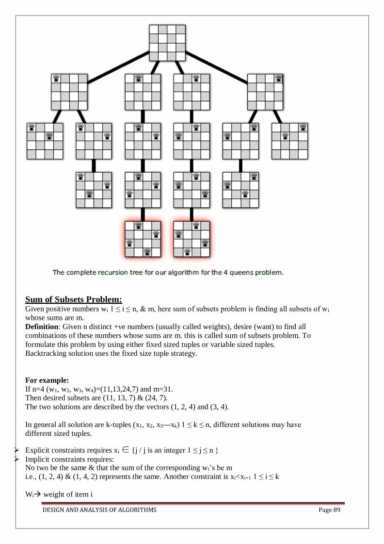
The backtracking solution vector (x1, x2, --- xn) xi ith visited

vertex of proposed cycle.


By using backtracking we need to determine how to compute the set of possible vertices for xk if

x1,x2,x3---xk-1 have already been chosen.

If k=1 then x1 can be any of the n-vertices. By using “NextValue” algorithm the recursive backtracking scheme to find all Hamiltoman

cycles.

This algorithm is started by 1st initializing the adjacency matrix G[1:n, 1:n] then setting x[2:n] to

zero & x[1] to 1, and then executing Hamiltonian (2)

Generating Next Vertex Finding all Hamiltonian Cycles

Algorithm NextValue(k) {

// x[1: k-1] is path of k-1 distinct vertices.

// if x[k]=0, then no vertex has yet been

assigned to x[k]

Repeat{

X[k]=(x[k]+1) mod (n+1); //Next vertex

If(x[k]=0) then return;

If(G[x[k-1], x[k]]≠0) then

{

For j:=1 to k-1 do if(x[j]=x[k]) then break;

//Check for distinctness

If(j=k) then //if true , then vertex is distinct

If((k<n) or (k=n) and G[x[n], x[1]]≠0)) Then

return ;

}

}

Until (false);

}

Algorithm Hamiltonian(k) {

Repeat{

NextValue(k); //assign a legal next value to

x[k]

If(x[k]=0) then return;

If(k=n) then write(x[1:n]);

Else Hamiltonian(k+1);

} until(false)

}

Branch & Bound

Branch & Bound (B & B) is general algorithm (or Systematic method) for finding optimal solution of

various optimization problems, especially in discrete and combinatorial optimization.

The B&B strategy is very similar to backtracking in that a state space tree is used to solve

a problem.

The differences are that the B&B method

Does not limit us to any particular way of traversing the tree.

It is used only for optimization problem

It is applicable to a wide variety of discrete combinatorial problem.

B&B is rather general optimization technique that applies where the greedy method &

dynamic programming fail.

It is much slower, indeed (truly), it often (rapidly) leads to exponential time complexities

in the worst case.

The term B&B refers to all state space search methods in which all children of the “E-

node” are generated before any other “live node” can become the “E-node”

Live node is a node that has been generated but whose children have not yet been

generated.

E-nodeis a live node whose children are currently being explored.


Dead node is a generated node that is not to be expanded or explored any further. All

children of a dead node have already been expanded.

Two graph search strategies, BFS & D-search (DFS) in which the exploration of a new

node cannot begin until the node currently being explored is fully explored.

Both BFS & D-search (DFS) generalized to B&B strategies.

BFSlike state space search will be called FIFO (First In First Out) search as the list of

live nodes is “First-in-first-out” list (or queue).

D-search (DFS) Like state space search will be called LIFO (Last In First Out) search

as the list of live nodes is a “last-in-first-out” list (or stack).

In backtracking, bounding function are used to help avoid the generation of sub-trees that

do not contain an answer node.

We will use 3-types of search strategies in branch and bound

1) FIFO (First In First Out) search

2) LIFO (Last In First Out) search

3) LC (Least Count) search

FIFO B&B:

FIFO Branch & Bound is a BFS. In this, children of E-Node (or Live nodes) are inserted in a queue.

Implementation of list of live nodes as a queue

Least() Removes the head of the Queue

Add() Adds the node to the end of the Queue

Assume that node ‘12’ is an answer node in FIFO search, 1st we take E-node has ‘1’


LIFO B&B:

LIFO Brach & Bound is a D-search (or DFS).

In this children of E-node (live nodes) are inserted in a stack

Implementation of List of live nodes as a stack

Least() Removes the top of the stack

ADD()Adds the node to the top of the stack.

Least Cost (LC) Search:

The selection rule for the next E-node in FIFO or LIFO branch and bound is sometimes “blind”. i.e.,

the selection rule does not give any preference to a node that has a very good chance of getting the

search to an answer node quickly.

The search for an answer node can often be speeded by using an “intelligent” ranking function. It is

also called an approximate cost function “Ĉ”.

Expended node (E-node) is the live node with the best Ĉ value.

Branching: A set of solutions, which is represented by a node, can be partitioned into mutually (jointly

or commonly) exclusive (special) sets. Each subset in the partition is represented by a child of the

original node.

Lower bounding: An algorithm is available for calculating a lower bound on the cost of any solution

in a given subset.

Each node X in the search tree is associated with a cost: Ĉ(X)

C=cost of reaching the current node, X(E-node) form the root + The cost of reaching an answer node

form X.

Ĉ=g(X)+H(X).

Example:

8-puzzle Cost function: Ĉ = g(x) +h(x)

where h(x) = the number of misplaced tiles

and g(x) = the number of moves so far Assumption:

move one tile in any direction cost 1.


Note: In case of tie, choose the leftmost node.


Travelling Salesman Problem:

Def:- Find a tour of minimum cost starting from a node S going through other nodes

only once and returning to the starting point S.

Time Conmlexity of TSP for Dynamic Programming algorithm is O(n22n) B&B algorithms for this problem, the worest case complexity will not be any better than O(n22n) but

good bunding functions will enables these B&B algorithms to solve some problem instances in much

less time than required by the dynamic programming alogrithm.

Let G=(V,E) be a directed graph defining an instances of TSP. Let

Cij cost of edge <i, j>

Cij =∞ if <i, j> ∉ E |V|=n total number of vertices.

Assume that every tour starts & ends at vertex 1.

Solution Space S= {1, Π , 1 / Π is a permutation of (2, 3. 4 --------------- n) } then |S|=(n-1)!

The size of S reduced by restricting S

Sothat (1, i1,i2,-----in-1, 1}∈ S iff <ij, ij+1>∈ E. O≤j≤n-1, i0-in=1 S can be organized into “State space tree”. Consider the following Example

State space tree for the travelling salesperson problem with n=4 and i0=i4=1 The

above diagram shows tree organization of a complete graph with |V|=4.

Each leaf node ‘L’ is a solution node and represents the tour defined by the path from the root to L.

Node 12 represents the tour.

i0=1, i1=2, i2=4, i3=3, i4=1

Node 14 represents the tour.

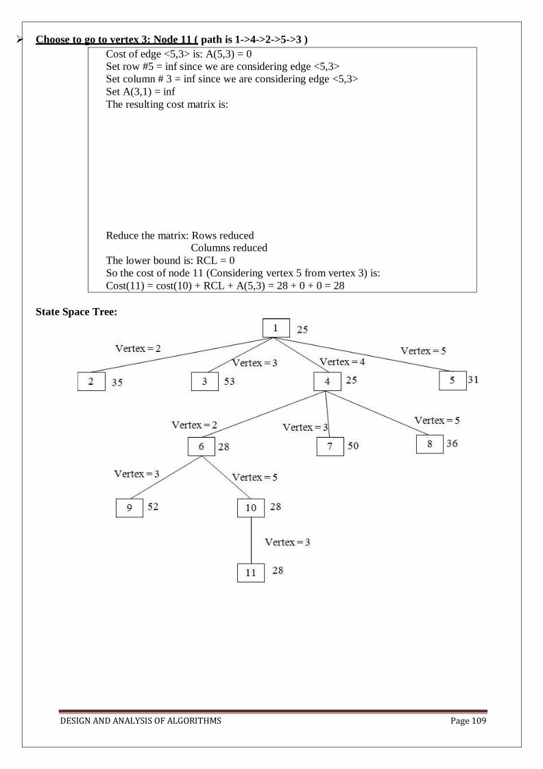
i0=1, i1=3, i2=4, i3=2, i4=1. TSP is solved by using LC Branch & Bound:

To use LCBB to search the travelling salesperson “State space tree” first define a cost function

C(.) and other 2 functions Ĉ(.) & u(.)

Such that Ĉ(r) ≤ C(r) ≤ u(r) for all nodes r.

Cost C(.) is the solution node1 with least C(.) corresponds to a shortest tour in G.


C(A)={Length of tour defined by the path from root to A if A is leaf Cost of a

minimum-cost leaf in the sub-tree A, if A is not leaf }

From1 Ĉ(r) ≤ C(r) then Ĉ(r) is the length of the path defined at node A. From previous example the path defined at node 6 is i0, i1, i2=1, 2, 4 & it consists edge of

<1,2> & <2,4>

Abetter Ĉ(r) can be obtained by using the reduced cost matrix corresponding to G.

A row (column) is said to be reduced iff it contains at least one zero & remaining entries

are non negative.

A matrix is reduced iff every row & column is reduced.

Given the following cost matrix:

The TSP starts from node 1: Node 1

Reduced Matrix: To get the lower bound of the path starting at node 1

Row # 1: reduce by 10

Row #2: reduce 2

Row #3: reduce by 2

Column 1: Reduce by 1 Row # 5: Reduce by 4 Row # 4: Reduce by 3:


- Cost of edge <1,2> is: A(1,2) = 10

- Set row #1 = inf since we are choosing edge <1,2>

- Set column # 2 = inf since we are choosing edge <1,2>

- Set A(2,1) = inf

- The resulting cost matrix is:

- The matrix is reduced:

- RCL = 0

- The cost of node 2 (Considering vertex 2 from vertex 1) is:

Cost(2) = cost(1) + A(1,2) = 25 + 10 = 35

The reduced cost is: RCL = 25

So the cost of node 1 is: Cost (1) = 25 The

reduced matrix is:

Choose to go to vertex 2: Node 2

Column 4: It is reduced.

Column 5: It is reduced.

Column 3: Reduce by 3 Column 2: It is reduced.


- Cost of edge <1,3> is: A(1,3) = 17 (In the reduced matrix

- Set row #1 = inf since we are starting from node 1


- Set A(3,1) = inf


Reduce the matrix: Rows are reduced

The columns are reduced except for column # 1:

Reduce column 1 by 11:

The lower bound is: RCL = 11

The cost of going through node 3 is:

cost(3) = cost(1) + RCL + A(1,3) = 25 + 11 + 17 = 53


Remember that the cost matrix is the one that was reduced at the starting vertex 1

Cost of edge <1,4> is: A(1,4) = 0

Set row #1 = inf since we are starting from node 1

Set column # 4 = inf since we are choosing edge <1,4>

Set A(4,1) = inf

The resulting cost matrix is:

Reduce the matrix: Rows are reduced




- Remember that the cost matrix is the one that was reduced at starting vertex 1

- Cost of edge <1,5> is: A(1,5) = 1

- Set row #1 = inf since we are starting from node 1


- Set A(5,1) = inf


Reduce the matrix:

Reduce rows:

Reduce row #2: Reduce by 2

Reduce row #4: Reduce by 3

Columns are reduced The lower bound is: RCL = 2 + 3 = 5 The cost of going

through node 5 is:

cost(5) = cost(1) + RCL + A(1,5) = 25 + 5 + 1 = 31

Columns are reduced



cost(4) = cost(1) + RCL + A(1,4) = 25 + 0 + 0 = 25


Cost of edge <4,2> is: A(4,2) = 3 Set row #4 = inf since we are considering edge <4,2>

Set column # 2 = inf since we are considering edge <4,2>

Set A(2,1) = inf


Reduce the matrix: Rows are reduced Columns are reduced



cost(6) = cost(4) + RCL + A(4,2) = 25 + 0 + 3 = 28

In summary:

So the live nodes we have so far are:

2: cost(2) = 35, path: 1->2

3: cost(3) = 53, path: 1->3

4: cost(4) = 25, path: 1->4

5: cost(5) = 31, path: 1->5

Explore the node with the lowest cost: Node 4 has a cost of 25

Vertices to be explored from node 4: 2, 3, and 5

Now we are starting from the cost matrix at node 4 is:

Choose to go to vertex 2: Node 6 (path is 1->4->2)


Cost of edge <4,3> is: A(4,3) = 12

Set row #4 = inf since we are considering edge <4,3>


Set A(3,1) = inf


Reduce the matrix: Reduce row #3: by 2:

Reduce column # 1: by 11

The lower bound is: RCL = 13 So the RCL of node 7 (Considering vertex 3 from vertex 4) is:

Cost(7) = cost(4) + RCL + A(4,3) = 25 + 13 + 12 = 50

Choose to go to vertex 3: Node 7 ( path is 1->4->3 )


Choose to go to vertex 5: Node 8 ( path is 1->4->5 ) Cost of

edge <4,5> is: A(4,5) = 0

Set row #4 = inf since we are considering edge <4,5> Set column # 5 = inf since we are considering edge <4,5> Set A(5,1) =

inf


Reduce the matrix: Reduced row 2: by 11

Columns are reduced The lower bound is: RCL = 11

So the cost of node 8 (Considering vertex 5 from vertex 4) is: Cost(8) =

cost(4) + RCL + A(4,5) = 25 + 11 + 0 = 36

In summary: So the live nodes we have so far are:

2: cost(2) = 35, path: 1->2

3: cost(3) = 53, path: 1->3

5: cost(5) = 31, path: 1->5

6: cost(6) = 28, path: 1->4->2

7: cost(7) = 50, path: 1->4->3

8: cost(8) = 36, path: 1->4->5


Vertices to be explored from node 6: 3 and 5



Cost of edge <2,3> is: A(2,3) = 11



Set A(3,1) = inf


The lower bound is: RCL = 2 +11 = 13 So the cost of node 9 (Considering vertex 3 from vertex 2) is:

Cost(9) = cost(6) + RCL + A(2,3) = 28 + 13 + 11 = 52

Choose to go to vertex 3: Node 9 ( path is 1->4->2->3 )

Reduce the matrix: Reduce row #3: by 2

Reduce column # 1: by 11


Cost of edge <2,5> is: A(2,5) = 0



Set A(5,1) = inf


Reduce the matrix: Rows reduced

Columns reduced


So the cost of node 10 (Considering vertex 5 from vertex 2) is:

Cost(10) = cost(6) + RCL + A(2,3) = 28 + 0 + 0 = 28

Choose to go to vertex 5: Node 10 ( path is 1->4->2->5 )

In summary: So the live nodes we have so far are:

2: cost(2) = 35, path: 1->2

3: cost(3) = 53, path: 1->3

5: cost(5) = 31, path: 1->5

7: cost(7) = 50, path: 1->4->3

8: cost(8) = 36, path: 1->4->5

9: cost(9) = 52, path: 1->4->2->3

10: cost(2) = 28, path: 1->4->2->5


Vertices to be explored from node 10: 3



Cost of edge <5,3> is: A(5,3) = 0



Set A(3,1) = inf


Reduce the matrix: Rows reduced Columns reduced


So the cost of node 11 (Considering vertex 5 from vertex 3) is:

Cost(11) = cost(10) + RCL + A(5,3) = 28 + 0 + 0 = 28

Choose to go to vertex 3: Node 11 ( path is 1->4->2->5->3 )

State Space Tree:


O/1 Knapsack Problem

What is Knapsack Problem: Knapsack problem is a problem in combinatorial optimization, Given a

set of items, each with a mass & a value, determine the number of each item to include in a collection

so that the total weight is less than or equal to a given limit & the total value is as large as possible.

O-1 Knapsack Problem can formulate as. Let there be n items, Z1 to Zn where Zi has value

Pi & weight wi. The maximum weight that can carry in the bag is m. All

values and weights are non negative.

Maximize the sum of the values of the items in the knapsack, so that sum of the weights must be less

than the knapsack’s capacity m.

The formula can be stated as

Xi=0 or 1 1 ≤ i ≤ n

To solve o/1 knapsack problem using B&B:

Knapsack is a maximization problem

Replace the objective function by the function to make it into a

minimization problem

The modified knapsack problem is stated as

Fixed tuple size solution space:

o Every leaf node in state space tree represents an answer for which

is an answer node; other leaf nodes are infeasible

o For optimal solution, define

for every answer node x

For infeasible leaf nodes,

For non leaf nodes

c(x) = min{c(lchild(x)), c(rchild(x))}

Define two functions c (x) and u(x) such that for every

node x,

cˆ(x) ≤ c(x) ≤ u(x)


Computing c (·) and u(·)

Algorithm ubound ( cp, cw, k, m )

{

// Input: cp: Current profit total

// Input: cw: Current weight total

// Input: k: Index of last removed item

// Input: m: Knapsack capacity

b=cp; c=cw; for i:=k+1 to n do{ if(c+w[i] ≤ m) then

{

c:=c+w[i]; b=b-p[i];

}

}

return b;

}


MODULE V:

NP-Hard and NP-Complete problems: Basic concepts, non deterministic algorithms, NP - Hard

and NPComplete classes, Cook’s theorem.

Basic concepts:

NP -) Nondeterministic Polynomial time

The problems has best algorithms for their solutions have “Computing times”, that cluster into

two groups

Group 1 Group 2

> Problems with solution time bound by

a polynomial of a small degree. > Problems with solution times not

bound by polynomial (simply non

polynomial )

> It also called “Tractable Algorithms” >

These are hard or intractable problems

> Most Searching & Sorting algorithms are polynomial time algorithms

>

None of the problems in this group

has been solved by any polynomial

> Ex: time algorithm

Ordered Search (O (log n)),

Polynomial evaluation O(n) > Ex:

Sorting O(n.log n) Traveling Sales Person O(n2 2n)

Knapsack O(2n/2)

No one has been able to develop a polynomial time algorithm for any problem in the 2nd group

(i.e., group 2)

So, it is compulsory and finding algorithms whose computing times are greater than polynomial

very quickly because such vast amounts of time to execute that even moderate size problems

cannot be solved.

Theory of NP-Completeness:

Show that may of the problems with no polynomial time algorithms are computational time

algorithms are computationally related.

There are two classes of non-polynomial time problems

1. NP-Hard

2. NP-Complete


DESIGN AND ANALYSIS OF ALGORITHMS (MODULE-VIII)

NP Complete Problem: A problem that is NP-Complete can solved in polynomial time if and only

if (iff) all other NP-Complete problems can also be solved in polynomial time.

NP-Hard: Problem can be solved in polynomial time then all NP-Complete problems can be solved

in polynomial time.

All NP-Complete problems are NP-Hard but some NP-Hard problems are not know to be NP-

Complete.

Nondeterministic Algorithms:

Algorithms with the property that the result of every operation is uniquely defined are termed as

deterministic algorithms. Such algorithms agree with the way programs are executed on a computer.

Algorithms which contain operations whose outcomes are not uniquely defined but are limited to

specified set of possibilities. Such algorithms are called nondeterministic algorithms.

The machine executing such operations is allowed to choose any one of these outcomes

subject to a termination condition to be defined later.

To specify nondeterministic algorithms, there are 3 new functions.

Choice(S) - ) arbitrarily chooses one of the elements of sets S

Failure ()-) Signals an Unsuccessful completion

Success ()-) Signals a successful completion.

Example for Non Deterministic algorithms:

Algorithm Search(x){

//Problem is to search an element x

//output J, such that A[J]=x; or J=0 if x is not in A

J:=Choice(1,n);

if( A[J]:=x) then {

Write(J); Success();

}

else{

write(0); failure();

Whenever there is a set of choices

that leads to a successful completion

then one such set of choices is

always made and the algorithm

terminates.

A Nondeterministic algorithm

terminates unsuccessfully if and

only if (iff) there exists no set of

choices leading to a successful

signal.

}



Nondeterministic Knapsack algorithm

Algorithm DKP(p, w, n, m, r, x){ p - ) given Profits

W:=0; w - ) given Weights

P:=0; n-) Number of elements (number of

for i:=1 to n do{ p or w)

x[i]:=choice(0, 1); m - ) Weight of bag limit

W:=W+x[i]*w[i]; P - ) Final Profit

P:=P+x[i]*p[i]; W- ) Final weight

}

if( (W>m) or (P<r) ) then Failure();

else Success();

}

The Classes NP-Hard & NP-Complete: For measuring the complexity of an algorithm, we use the input length as the parameter. For example,

An algorithm A is of polynomial complexity p() such that the computing time of A is O(p(n)) for

every input of size n.

Decision problem/ Decision algorithm: Any problem for which the answer is either zero or one is

decision problem. Any algorithm for a decision problem is termed a decision algorithm.

Optimization problem/ Optimization algorithm: Any problem that involves the identification of

an optimal (either minimum or maximum) value of a given cost function is known as an

optimization problem. An optimization algorithm is used to solve an optimization problem.

P-) is the set of all decision problems solvable by deterministic algorithms in polynomial time.

NP-) is the set of all decision problems solvable by nondeterministic algorithms in polynomial

time.

Since deterministic algorithms are just a special case of nondeterministic, by this we concluded

that P ⊆ NP

Commonly believed relationship between P & NP



The most famous unsolvable problems in Computer Science is Whether P=NP or P≠NP In

considering this problem, s.cook formulated the following question.

If there any single problem in NP, such that if we showed it to be in ‘P’ then that would imply that

P=NP.

Cook answered this question with

Theorem: Satisfiability is in P if and only if (iff) P=NP

-)Notation of Reducibility

Let L1 and L2 be problems, Problem L1 reduces to L2 (written L1 α L2) iff there is a way to solve

L1 by a deterministic polynomial time algorithm using a deterministic algorithm that solves L2 in

polynomial time

This implies that, if we have a polynomial time algorithm for L2, Then we can solve L1 in

polynomial time.

Here α-) is a transitive relation i.e., L1 α L2 and L2 α L3 then L1 α L3

A problem L is NP-Hard if and only if (iff) satisfiability reduces to L ie., Statisfiability α L

A problem L is NP-Complete if and only if (iff) L is NP-Hard and L Є NP

Commonly believed relationship among P, NP, NP-Complete and NP-Hard Most

natural problems in NP are either in P or NP-complete. Examples of NP-complete problems:

> Packing problems: SET-PACKING, INDEPENDENT-SET.

> Covering problems: SET-COVER, VERTEX-COVER.

> Sequencing problems: HAMILTONIAN-CYCLE, TSP.

> Partitioning problems: 3-COLOR, CLIQUE. > Constraint satisfaction problems: SAT, 3-SAT.

> Numerical problems: SUBSET-SUM, PARTITION, KNAPSACK.



Cook’s Theorem: States that satisfiability is in P if and only if P=NP If P=NP

then satisfiability is in P

If satisfiability is in P, then P=NP To do this

> A-) Any polynomial time nondeterministic decision algorithm.

I-)Input of that algorithm

Then formula Q(A, I), Such that Q is satisfiable iff ‘A’ has a successful

termination with Input I.

> If the length of ‘I’ is ‘n’ and the time complexity of A is p(n) for some polynomial

p() then length of Q is O(p3(n) log n)=O(p4(n))

The time needed to construct Q is also O(p3(n) log n).

> A deterministic algorithm ‘Z’ to determine the outcome of ‘A’ on any input ‘I’

Algorithm Z computes ‘Q’ and then uses a deterministic algorithm for the satisfiability

problem to determine whether ‘Q’ is satisfiable.

> If O(q(m)) is the time needed to determine whether a formula of length ‘m’ is

satisfiable then the complexity of ‘Z’ is O(p3(n) log n + q(p3(n)log n)).

> If satisfiability is ‘p’, then ‘q(m)’ is a polynomial function of ‘m’ and the

complexity of ‘Z’ becomes ‘O(r(n))’ for some polynomial ‘r()’.

> Hence, if satisfiability is in p, then for every nondeterministic algorithm A in NP, we can

obtain a deterministic Z in p.

By this we shows that satisfiability is in p then P=NP

Date post:	16-Oct-2021
Category:	Documents
Upload:	others
View:	2 times
Download:	0 times

NOTES ON DESIGN AND ANALYSIS OF ALGORITHMS B.TECH II …

Documents