Notes on Discrete Exterior Calculus Andrew Gillette August 27, 2009 These notes are aimed at mathematics graduate students familiar with introductory algebraic and differential topology. The notes were written under the guidance of Dr. John Luecke and Dr. Jennifer Mann as part of NSF Research Training Grant DMS-0636643 at the University of Texas at Austin. Contents 1 Introduction 2 1.1 Differential Forms for Physical Models .......................... 2 1.2 What is Discrete Exterior Calculus? ........................... 3 1.3 Relevance to Biological Modeling ............................. 3 1.4 History of Discrete Exterior Calculus ........................... 3 1.5 Comparison to Finite Element Methods ......................... 4 2 Notation and Background 6 2.1 Manifold-like Simplicial Complexes ............................ 6 2.2 Orientation of Simplicial Complexes ........................... 7 2.3 Dual Complexes ...................................... 8 2.4 Orientation of Dual Complexes .............................. 9 2.5 Discrete Differential Forms ................................ 9 2.6 Discrete Exterior Derivative ................................ 10 2.7 Projection and Interpolation of Discrete Forms ..................... 11 2.8 Whitney Interpolatory Forms ............................... 12 2.9 Discrete Hodge Star .................................... 12 2.10 Discrete Coderivative .................................... 14 2.11 Discrete Vector Fields ................................... 14 2.12 Flat Operators: From Vector Fields to Forms ...................... 14 2.13 Sample Calculation ..................................... 16 3 Darcy flow example 17 3.1 Step 1: Governing Equations ............................... 17 3.2 Step 2: Domain, Variable, and Operator Replacement ................. 18 3.3 Step 3: Linear System ................................... 19 3.4 Hodge Star for Darcy Flow ................................ 20 3.5 The importance of well-centerdness ............................ 20 3.6 Conclusion and Future Work ............................... 21 1
Transcript
Notes on Discrete Exterior Calculus
Andrew Gillette
August 27, 2009
These notes are aimed at mathematics graduate students familiar with introductory algebraicand differential topology. The notes were written under the guidance of Dr. John Luecke and Dr.Jennifer Mann as part of NSF Research Training Grant DMS-0636643 at the University of Texasat Austin.
Differential forms are often presented to mathematicians as the underpinning of modern calculus.The dx familiar to calculus students, for example, is revealed to be the most basic type of 1-form.Higher order forms such as the 2-form dA and the 3-form dV are often thought of in terms of theircomposite 1-forms, suggesting that 1-forms are the essential building blocks of differential calculus.Delving into applied mathematics, however, one discovers that certain physical phenomena are mostaccurately described by differential forms of specific dimensions and to treat them as products of1-forms or as anything else would greatly complicate their analysis.
While this has been acknowledged for some time in theoretical circles (including, for example,works by both Maxwell and Kelvin in the late 1800s) it has only recently gained traction in themodeling and simulation communities. With the advent of high-speed computing and high-levelprogramming languages, engineers are now incorporating more differential topology concepts intotheir programs so that their models can benefit from a rigorous theoretical foundation.
The importance of differential forms is perhaps most evident in electromagnetics research wherethe main quantities of interest - potential, electric fields, magnetic fields, and current density - arebest described as forms of dimension 0, 1, 2, and 3, respectively. (For those unfamiliar with theseterms, a useful review of electromagnetics is the textbook [21] by Griffiths.) To see why these aretruly different-dimensional phenomena, we can begin by looking at their units as shown in Table 1.
Table 1: Units Used in ElectromagneticsQuantity Symbol Unit DimensionElectric Potential φ V 0Electric Field E V/m 1Magnetic Field B (V · s)/m2 2Current Density (3D) ρ A/m3 3
Each variable is quantified relative to a different dimensional unit: φ is per point, E is perlength, B is per area, and ρ is per volume. This dimensionality analysis extends to the auxiliarymagnetic field H which is measured in A/m, a per length measurement, reflecting its complementaryrelationship to B.
Dimensionality, however, is only a component of differential form based modeling. We take Eas an example of how forms can more faithfully represent physical phenomena than, for example,vector fields. When a charge at a point x moves to point x + v(x), energy is transferred by Edepending on the displacement v(x). This energy transfer is called work and experiments showthat the work done is proportional to v(x). Therefore, the value of E at x should be a linearfunction of v(x). In the language of differential forms, this is the same as saying E should be alinear functional on the tangent space at x, i.e. a 1-form.1
We note that the information encoded by a 1-form can be captured by a vector field in acanonical way. The flat operator [ converts vector fields to forms and the sharp operator ] doesthe reverse [1]. In our example, the vector representing E at x is defined to be ~w(x) such that thework done by E on a charge with displacement v(x) is given by w(x) · v(x). The linear functionalrepresenting E at x is defined to be (w(x),−) where (−,−) indicates the dot product.
The motivation of using forms for modeling is thus based on the mathematical relationships1For a primer on differential geometry applied to electromagnetism, see [11].
2
implied by differential topology that cannot be expressed in the language of vector fields alone.Since computational modeling must be done in a discrete manner, we turn to discrete exteriorcalculus to guide the discretization of form models.
1.2 What is Discrete Exterior Calculus?
Discrete Exterior Calculus (DEC) is an attempt to create from scratch a discrete theory of differ-ential geometry and topology whose definitions and theorems mimic their smooth counterparts. Amanifold is discretized as a simplicial complex and discrete k-forms are defined to be cochains onthe k-dimensional simplices. The exterior derivative operator d is discretized as ∂T , the transpose ofthe adjacency matrix in the appropriate dimension. Other discrete operators have more elaboratediscretizations.
The main application of DEC, aside from any theoretical interest, is the creation of discreteoperators for use in numerical methods for Partial Differential Equations (PDEs). While discreteoperators have appeared in the literature for some time, DEC offers a unified approach to theirconstruction, backed by the rigor of differential topology. The main steps in such an approach areas follows.
1. Write out the PDE in terms of smooth differential operators.
2. Replace the smooth domain, variables, and operators by their DEC counterparts.
3. Use DEC-based analysis to set up an appropriate linear system of equations.
The resulting linear system can then be solved by existing numerical methods to approximatesolutions to the PDE.
1.3 Relevance to Biological Modeling
While DEC-based methods are useful to many modeling problems involving PDEs, they are espe-cially relevant to PDEs arising in biological modeling at the molecular scale. Today, many methodsexist for imaging molecules at scales as small as an Angstrom (1 A= 10−10 m) and creating com-putational models of them. These discrete 2- and 3-manifolds then become the domains used insimulations of biological activity not observable by any direct method. Events such as proteinconstruction and folding, virus capsid assembly, and DNA knotting and unknotting occur at suchsmall physical scales and rapid time scales that no known or theoretical device can record them asthey are happening. However, these types of activity are governed by various PDEs, depending onthe scale and context, hence a rigorous analysis suitable to large datasets and undulating shapes isrequired. DEC provides the theoretical backing to move these types of computational models fromad hoc approximations to robust error-analyzed algorithms.
1.4 History of Discrete Exterior Calculus
As mentioned previously, it was recognized for some time that certain physical phenomena, such asthose observed in electromagnetics, are well described by differential forms. In the 1980s, researchersbegan to consider how this characterization could or should be used in computational models [19, 6].As individual techniques advanced, attempts were made to unify various discretization methods,such the work of Hyman and Shashkov [28, 27, 29] on natural discretizations of the div, curl, andgrad operators. Work by Hiptmair [23] and Bossavit [11, 13, 14] began to lay the foundation incomputational electromagnetics for a more unified theory.
3
Treating discretization of differential operators entirely through the lens of exterior calculus,however, is a more recent development. For a thorough introduction to DEC theory, as well as moreexpansive descriptions of prior work, see Hirani [25] and Desbrun et al. [17]. DEC theory has beenemployed by an increasing number of authors in recent years to create mimetic operators [8, 34],develop multigrid solvers [7], solve Darcy flow problems [26], discretize Einstein’s equations forgeneral relativity [20], and geometrize elasticity [36]. Additionally, Lawrence Livermore NationalLaboratory has recongized DEC as the essential underpinning to its next-generation numericalmethods and released a lengthy report detailing their initial implementation [16].
1.5 Comparison to Finite Element Methods
To put DEC-based PDE solvers in context, we compare them to finite element methods (FEMs),now an industry standard in applications and an area of active research. We illustrate the similari-ties and differences between the methods on the following general PDE problem. Given a boundeddomain Ω ⊂ Rn, find u ∈ V such that
Lu = f on Ω, (1)
where L is a linear operator, f ∈ L2(Ω), and V is the appropriate solution space for the problem.For the moment, we do not specify boundary conditions. The Galerkin finite element methodbegins by putting (1) into a weak form. Observe that for any v ∈ V we can compute∫
Ω(Lu)v =
∫Ωfv.
Define a bilinear form a : V × V → R capturing the computation of the integral on the left andtreat f as a functional (f, ·)L2 on V . Then the weak form of (1) is to find u ∈ V such that
a(u, v) = (f, v)L2 ∀v ∈ V. (2)
We clarify this reduction by a brief example.
Example 1.1. (from [15]) Consider the PDE
−d2u
dx2= f in (0, 1) ⊂ R1 with u(0) = 0.
The solution space isV := v ∈W 1
2 (0, 1) : v(0) = 0,
where W 12 (Ω) is the Sobolev space of functions in L2(Ω) whose first derivative is also in L2(Ω).
Integrating against v ∈ V gives ∫ 1
0u′′vdx =
∫ 1
0fvdx,
which after integration by parts and the boundary condition becomes∫ 1
0u′v′dx =
∫ 1
0fvdx.
Therefore, we set the bilinear form a : V × V → R in this case to be
a(u, v) :=∫ 1
0u′v′dx.
4
It can be shown that a is a symmetric bilinear form on W 12 (0, 1) and coercive on V . It is not,
however, an inner product on W 12 (0, 1) since a(1, 1) = 0 (where 1 denotes the function which is
identically 1 on (0, 1)). ♦
To discretize this problem, we choose an appropriate finite dimensional subspace Vh ⊂ V andseek an answer to the following problem: find u ∈ Vh such that
a(u, v) = (f, v)L2 ∀v ∈ Vh. (3)
Since Vh is finite-dimensional, we can fix a basis φi : 1 ≤ i ≤ n of Vh. Write u =∑n
j=1 Ujφj ,Kij = a(φj , φi) and Fi = (f, φi). Set U = (Uj), K = (Kij) F = (Fi). Then solving (3) is the sameas solving the matrix equation
KU = F. (4)
A proof and detailed discussion of this reduction can be found in [15].A significant amount of care goes into the selection of Vh to ensure that the method is both
well-posed and stable. Well-posed means the system (3) has a unique solution uh. The moresubtle question of stability asks whether uh bears any relation to the true solution u. The methodis called stable if there exists a constant C > 0 independent of h such that
||u− uh||V ≤ C infwh∈Vh
||u− wh||V .
In other words, a method is stable if the error between the solution u to (2) and the solution uh to(3) is bounded above uniformly by a constant multiple of the minimal approximation error for Vh.The famous Babuska inf-sup condition [5] is often used to simultaneously prove both well-posednessand stability of a finite element method and hence provide an a priori bound on solver error. Manypapers have been published proving this condition for a specific finite element scheme or class ofschemes. Recently, Arnold, Falk and Winther [3] have presented a unified characterization of stablesolution spaces for certain classes of PDEs using the theory of differential forms.
The method of Discrete Exterior Calculus is an alternative approach which focuses on correctlydiscretizing the operator L instead of the solution space V . The viewpoint provided by differentialgeometry and topology reveals how this ought to be done. Common operators such as grad, curl,and div are all manifestations of the exterior derivative operator d in dimensions 1, 2, and 3,respectively. Equations relating quantities of complementary dimensions, such as the constitutiverelations in Maxwell’s equations, involve a Hodge star operator ∗ which provides the canonicalmapping. The Laplacian operator ∆ can be written as δd+dδ where δ is the coderivative operator,defined by δ := ∗d∗. Each operator has a discrete version designed to mimic the properties of itssmooth counterpart. The discrete versions of the operators are written as matrices whose entriesdepend only on the topology and geometry of the mesh of Ω. We will give the formulation of thesematrices in detail in Section 2.
To solve (1), an analysis is made as to the dimension of u as a k-form based on either theproblem context (as described in Section 1.1) or the type of operator acting on u. The div operatorin 3D, for example, acts on 2-forms while grad acts on 0-forms. The variable u is replaced by avector ~u with one entry for each k-simplex in the mesh of Ω and the operator L is replaced by itsdiscrete counterpart, written as a matrix L. The load data f is converted to a vector ~f accordingly.This yields the equation
L~u = ~f, (5)
which can then be solved by linear methods. The Whitney interpolant (see Section 2.8) is commonlyused to compute values for u away from the k-simplices in the simplicial complex approximatingΩ.
5
Discrete Exterior Calculus can also be used to solve (2), the weak version of the problem.Suppose that the domain Ω is a primal mesh2 with N vertices w1, . . . , wN . Let ui := u(wi). Forany v ∈ V , let vi := v(wi). Then we can write
a(u, v) =N∑
k,m=1
Lkmukvm
where L is a real symmetric matrix constructed based on the same methodology described above.We also need to approximate the right side of equation (2), that is, the L2 inner product. For this,we need a matrix M such that
(u, v)L2 ≈∑k,m
Mkmukvm. (6)
Let χ denote the characteristic function of Ω so that χi = χ(wi) = 1. If (6) is to hold, then inparticular we should have∑
k,m
Mkm =∑k,m
Mkmχkχm ≈ (χ, χ)L2 =∫
Ω1 = |Ω|
where |Ω| is the Lebesgue measure of Ω. Since |Ω| indicates the “quantity” or “size” of Ω in somesense, the matrix M is often referred to as the mass matrix. Combining the above statements andletting fi := f(wi), we find that the discrete analogue of (2) is∑
k,m
Lkmukvm =∑k,m
Mkmfkvm ∀v ∈ V.
Remark 1.2. This formulation of discrete operators is only applicable when u and v are character-ized by their values on the vertices of the mesh Ω. In some instances, it may be more appropriateto characterize u or v by their values on edges, faces, or some other combinatorial subset of Ω. InSection 3, we discuss such an example in detail that arises from modeling Darcy flow. ♦
2 Notation and Background
2.1 Manifold-like Simplicial Complexes
In algebraic topology, manifolds are discretized using simplicial complexes, a notion which guidesthe entire theory of DEC. We state the definition of simplicial complex here, along with supportingdefinitions to be used throughout. These definitions can be found in algebraic topology texts suchas Armstrong [2] or Hatcher [22] or in Hirani’s thesis [25].
Definition 2.1. A p-simplex σp is the convex hull of p + 1 geometrically independent pointsv0, . . . , vp ∈ RN . That is
σp =
x ∈ RN : x = σpi=0µivi where µi ≥ 0 and
n∑i=0
µi = 1
.
Any simplex spanned by a (proper) subset of v0, . . . , vp is called a (proper) face of σp. Theunion of the proper faces of σp is called its boundary and denoted Bd(σp). The interior of σp isInt(σp) = σp\Bd(σp). Note that Int(σ0)=σ0. The volume of σp is denoted |σp|. Define |σ0| = 1.♦
2See Definition 2.9.
6
We will indicate that a simplex has dimension p with a superscript, e.g. σp, and will indexsimplices of any dimension with subscripts, e.g. σi.
Definition 2.2. A simplicial complex K in RN is a collection of simplices in RN such that
1. Every face of a simplex of K is in K.
2. The intersection of any two simplices of K is either a face of each of them or it is empty
The union of all simplices of K treated as a subset of RN is called the underlying space of K andis denoted by |K|. ♦
Definition 2.3. A simplicial complex of dimension n is called a manifold-like simplicial com-plex if and only if |K| is a C0-manifold, with or without boundary. More precisely
1. All simplices of dimension k with 0 ≤ k ≤ n− 1 must be a face of some simplex of dimensionn in K.
2. Each point on |K| has a neighborhood homeomorphic to Rn or n-dimensional half-space.
♦
Remark 2.4. Since DEC is meant to treat discretizations of manifolds, we will assume all simplicialcomplexes are manifold-like from here forward. We note that |K| is thought of as a piecewiselinear approximation of a smooth manifold M . Formally, this is taken to mean that there exists ahomeomorphism h between |K| and M such that h is isotopic to the identity. This homeomorphismwill become relevant when we discuss different methods for defining a discrete Hodge Star in Section2.7. In applications, however, knowing h or M explicitly may be irrelevant or impossible as K oftenencodes everything known about M . This emphasizes the usefulness of DEC as a theory built fordiscrete settings. ♦
2.2 Orientation of Simplicial Complexes
We now review how to orient a simplicial complex K. The definitions and conventions adoptedhere are taken from Hirani [25].
Definition 2.5. Define two orderings of the vertices of a simplex σp (p ≥ 1) to be equivalent if theydiffer by an even permutation. Thus, there are two equivalence classes of orderings, each of whichis called an orientation of σp. If σp is written as [v0, . . . , vp], the orientation of σp is understoodto be the equivalence class of this ordering. ♦
Definition 2.6. Let σp = [v0, . . . , vp] be an oriented simplex with p ≥ 2. This gives an inducedorientation on each of the (p−1)-dimensional faces of σp as follows. Each face of σp can be writtenuniquely as [v0, . . . , vi, . . . , vp], where vi means vi is omitted. If i is even, the induced orientationon the face is the same as the oriented simplex [v0, . . . , vi, . . . , vp]. If i is odd, it is the opposite. ♦
We note that this formal definition of induced orientation agrees with the notion of orientationinduced by the boundary operator to be defined later. In that setting, a 0-simplex can also receivean induced orientation.
Remark 2.7. We will need to be able to compare the orientation of two oriented p-simplices σp
and τp. This is possible only if at least one of the following conditions holds:
7
1. There exists a p-dimensional affine subspace P ⊂ RN containing both σp and τp.
2. σp and τp share a face of dimension p− 1.
In the first case, write σp = [v0, . . . , vp] and τp = [w0, . . . , wp]. Note that v1−v0, v2−v0, . . . , vp−v0and w1 −w0, w2 −w0, . . . , wp −w0 are two ordered bases of P . We say σp and τp have the sameorientation if these bases orient P the same way. Otherwise, we say they have opposite orientations.In the second case, σp and τp are said to have the same orientation if the induced orientation onthe shared p− 1 face induced by σp is opposite to that induced by τp. ♦
Definition 2.8. Let σp and τp with 1 ≤ p ≤ n be two simplices whose orientations can becompared, as explained in Remark 2.7. If they have the same orientation, we say the simpliceshave a relative orientation of +1, otherwise −1. This is denoted as sgn(σp, τp) = +1 or −1,respectively. ♦
Definition 2.9. A manifold-like simplicial complex K of dimension n is called an orientedmanifold-like simplicial complex if adjacent n-simplices agree on the orientation of their sharedface. Such a complex will be called a primal mesh from here forward. ♦
2.3 Dual Complexes
Dual complexes are defined relative to a primal mesh. While they represent the same subset ofRN as their associated primal mesh, they create a different data structure for the geometricalinformation and become essential in defining the various operators needed for DEC. Circumcentricsubdivision is the preferred method for defining a dual complex as it best supports the theoreticalconstructs. We will look at an example in Section 2.13 to see how the choice of subdivision methodimpacts numerical calculation.
Definition 2.10. The circumcenter of a p-simplex σp is given by the center of the unique p-sphere that has all p+ 1 vertices of σp on its surface. It is denoted c(σp). A simplex σp is said tobe well-centered if c(σp) ∈ Int(σp). A well-centered simplicial complex is one in which allsimplices (of all dimensions) in the complex are well-centered. ♦
Definition 2.11. Let K be a well-centered primal mesh of dimension n and let σp be a simplexin K. The circumcentric dual cell of σp, denoted D(σp), is given by
D(σp) :=n−p⋃r=0
⋃σp≺σ1≺···≺σr
Int(c(σp)c(σ1) . . . c(σr)).
To clarify, the inner union is taken over all sequences of r simplices such that σp is the first elementin the sequence and each sequence element is a proper face of its successor. For r = 0, this is to beinterpreted as the sequence σp only. The closure of the dual cell of σp is denoted D(σp) and calledthe closed dual cell. We will also use the notation ? to indicate dual cells, i.e.
?σ := D(σ).
Each (n− p)-simplex on the points c(σp), c(σ1), . . . , c(σr) is called an elementary dual simplexof σp. The collection of dual cells is called the dual cell decomposition of K and denoted D(K)or ?K. ♦
Some examples of dual cells are shown in Figure 1 and discussed in its caption. Note that thedual cell decomposition forms a CW complex (see Munkres [31] for more on this).
8
Figure 1: Figure 2.3 from Hirani [25]. The solid black lines form a simplicial complexK of dimension2. The dotted lines show how subdivision refines the complex. A few dual cells are shown in red.The red line segments are the duals of the black 1-simplices they intersect. The red region is thedual cell of the vertex it surrounds. The red vertex is the dual of the triangle in which it sits.
2.4 Orientation of Dual Complexes
Orientation of the dual complex must be done in a such a way that it “agrees” with the orientationof the primal context. This can be done canonically since a primal simplex and any of its elementarydual simplices have complementary dimension and live in orthogonal affine subspaces of RN . Wemake this more precise and fix the necessary conventions with the following definitions.
Definition 2.12. Let K be a primal mesh with simplices σ0 ≺ σ1 ≺ · · · ≺ σn and let σp be one ofthese simplices with 1 ≤ p ≤ n− 1. The orientation of the elementary dual simplex with verticesc(σp), . . . , c(σn) is s[c(σp), . . . , c(σn)] where s ∈ −1,+1 is given by the formula
s := sgn([c(σ0), . . . , c(σp)], σp
)× sgn
([c(σ0), . . . , c(σn)], σn
).
The sgn function was defined in Definition 2.8. For p = n, the dual element is a vertex which hasno orientation. For p = 0, define s := sgn
([c(σ0), . . . , c(σn)], σn
). ♦
The above definition serves to orient all the elementary dual simplices associated to σp and henceall simplices in a dual cell decomposition. Further, the orientations on the elementary dual simplicesinduce orientations on the boundaries of dual cells in the same manner as given in Definition 2.6.
2.5 Discrete Differential Forms
Definition 2.13. Let K be a primal mesh of a smooth compact n-manifold Ω. Let Kk denote thek-simplices of K. A k-chain c is a linear combination of the elements of Kk:
c =∑σ∈Kk
cσσ,
where cσ ∈ R. The set of all such chains form the vector space of k-chains is denoted Ck. It hasdimension |Ck| equal to the number of elements of Kk. A k-chain c is represented as column vectorof length |Ck|. The chains of the dual complex ?K are, similarly, linear combinations of k-cells of?K. ♦
9
Definition 2.14. A k-cochain ω is the dual of a k-chain:
ω : Ck → R via c 7→ ω(c),
where ω is a linear mapping. It is represented as a column vector of length |Ck| so that the action ofω on a k-chain c is the matrix multiplication ωT c, yielding the scalar ω(c). The set of all cochainsis denoted Ck. ♦
Cochains are the discrete analogues of differential forms as they can be evaluated over anyk-dimensional subspace. To make this precise, we define the integration of a cochain over a chainto be the evaluation of the cochain as a function.
Definition 2.15. The integral of a k-cochain ω over a k-chain c is defined to be∫cω := ωT c = ω(c).
Hence, the integration of ω over c is exactly the same as the evaluation of ω on c. We will alsodenote this pairing of cochain with chain using bracket notation:
< ω, c >:= ω(c).
♦
2.6 Discrete Exterior Derivative
To define a discrete version of the various differential operators, we first need a discrete exteriorderivative. We will use the alternative definition of the smooth exterior derivative to motivate ourdiscrete definition. First we define the boundary operator in the discrete case.
Definition 2.16. The kth boundary operator denoted by ∂ takes a k-chain to its (k− 1)-chainboundary. It is defined by its action on an oriented k-simplex:
∂[v0, v1, · · · , vk] :=k∑i=0
(−1)i[v0, · · · , vi, · · · , vk]
where vi indicates that vi is omitted. The boundary operator is represented as a matrix of size|Ck−1| × |Ck| so that the action of ∂ on a k-chain c is the usual matrix multiplication ∂c. ♦
Definition 2.17. Let ω be a k-cochain. The kth discrete exterior derivative of ω is thetranspose of the (k + 1)st boundary operator:
Dk = ∂T .
This is also referred to in the literature as the coboundary operator. It is represented as amatrix of size |Ck+1|× |Ck| so that the action of Dk on a k-chain c is the usual matrix multiplicationDc := ∂T c. ♦
The discrete exterior derivative satisfies the discrete version of Stokes’ theorem.
Lemma 2.18. Let ω be a k-cochain and c ∈ Ck+1 any (k + 1)-chain. Then∫cDkω =
∫∂cω.
10
Proof. By definition 2.15 we see that∫∂cω = ωT∂c = (∂Tω)T c = (Dkω)T c =
∫cDkω.
Remark 2.19. The discrete exterior derivative d as defined operates on primal cochains, howeverwe will need to understand how it acts on dual cochains as well. According to [18] (Section 4.5),the relationship is the following:
DDualn−k = (−1)k(DPrimal
k−1 )T .
The negative sign comes from the orientation on the dual mesh induced by the orientation on theprimal mesh. ♦
2.7 Projection and Interpolation of Discrete Forms
To pass the rest of our theory between smooth and discrete settings, we will need a homeomorphismh : K → Ω between our smooth and discrete spaces as well as maps between the smooth k-formsΛk and the discrete k-forms Ck. These maps are denoted
Rk : Λk → Ck and Ik : Ck → Λk
which we will now define.
Definition 2.20. Fix a primal mesh K of an n-manifold Ω with an accompanying homeomorphismh : K → Ω. The kth deRham map Rk : Λk → Ck is defined as follows. Given ω ∈ Λk and c ∈ Cka chain, define
(Rkω)(c) :=∫h(c)
ω.
♦
In words, the evaluation of the k-cochain Rkω on k-chain c ∈ K is the integral of the k-form ωover h(c), the image of the c in Ω.
Lemma 2.21. The map R satisfies Rd = DR, i.e. the following is a commutative diagram:
Λk
Rk
dk // Λk+1
Rk+1
Ck
Dk // Ck+1
The map Ik : Ck → Λk is called an interpolation map and has no canonical choice since R isnot invertible. We can require, however, that Ik be chosen such that:
• RI = id (consistency)
• IR = id +O(hs) (approximation)
where h ∈ R>0 is the partition size of the mesh and s ∈ R>0 is the approximation order. Note thatfor the Whitney interpolation maps we define next, s = 1.
11
2.8 Whitney Interpolatory Forms
The Whitney map is a commonly used interpolation operator. The idea is to construct a basisof k-forms whose support is defined relative to a particular k-simplex. The namesake of theseforms is Hassler Whitney, who first described them in 1957 in [35] (page 139). Bossavit explainsthe relevance of Whitney forms to “mixed methods” of finite elements in [9]. We will state thegeneral definition of a Whitney form first (as given in [10]) and then give the specific definitionsfor Whitney forms on subsets of a tetrahedron.
Given a primal mesh K of Ω, fix a vertex i in the mesh and let x be a point in one of thetetrahedra that shares vertex i. Let λi(x) be the barycentric weight of the point x in its tetrahedronwith respect to vertex i. Note that λi is continuous and defined on shared edges and faces withvertex i and can be extended to a function on all of Ω by defining it to be zero outside the tetrahedracontaining x.
Definition 2.22. Let τ := [v0, . . . , vk] denote a k-simplex and λ0, . . . , λk the barycentric coordinatefunctions of τ . The Whitney form ητ ∈ Λk associated to this simplex is defined by
ητ := k!k∑i=0
(−1)iλidλ0 ∧ . . . ∧ dλi ∧ . . . ∧ dλk
where dλi indicates that dλi is omitted. Given a k-cochain ω ∈ Ck, its Whitney interpolantI(ω) is
I(ω) :=∑τ∈Ck
ω(τ)ητ
♦
We compute examples of Whitney forms in Section 2.13.
2.9 Discrete Hodge Star
Next we want to define a discrete Hodge Star. Recall that in the smooth setting, ∗ maps k-forms to(n− k)-forms and satisfies the relationship α ∧ ∗β = (α, β)µ where µ is the volume form. Thus, inthe discrete setting, ∗ should map k-cochains to (n− k)-cochains and satisfy a similar relationship.We therefore have two choices on how to proceed in our definitions:
1. Define an inner product of two cochains and induce a discrete Hodge Star.
2. Define a discrete Hodge Star and induce an inner product.
We will examine each in turn. First we consider how one could define an inner product of twocochains and induce a discrete Hodge Star.
Definition 2.23. Let a, b ∈ Ck. The inner product of k-cochains is defined by (a, b)Ck :=(Ia, Ib)Λk . ♦
This definition allows for two possible discrete Hodge stars.
Definition 2.24. The natural discrete ∗ is given byn∗:= R ∗ I so that
(a,n∗ b)Ck = (Ia, IR ∗ Ib)Λk
12
which impliesn∗ R = R∗. The derived discrete ∗ is induced by
∫a∧ d∗ b :=
∫Ia ∧ ∗Ib so that
(a,d∗ b)Ck = (Ia, ∗Ib)Λk
which implies∫a∧ d∗ a = (a, a) for a ∈ Ck. ♦
Unfortunately, the implied property listed after each definition is not implied by the otherdefinition. That is,
d∗ R = R ∗ +O(hs) and∫a∧ n∗ a = (a, a) + O(hs). This is elucidated further
by Bochev and Hyman [8]. The difficulty in this approach from a computational standpoint is indefining an inner product that can be evaluated over non-flat triangulations.
The alternative option to this route is to define a discrete Hodge Star such that an inner productcan be induced. Observe that an (n−k)-cochain is defined by its action on (n−k)-chains, howeverthere is no canonical way to associate a k-simplex to an (n− k)-simplex in the same primal mesh.On the other hand, there is a very natural way to associate a k-simplex in a primal mesh to an(n− k)-cell in the dual complex and vice versa. Hence the discrete Hodge star will be a map fromdiscrete primal k-forms to discrete dual (n− k)-forms.
Definition 2.25. The kth discrete Hodge Star for a primal mesh K is a map from Ck(K) toCn−k(?K) represented by a matrix Mk of size |Ck| × |Ck|. The formulation of the entries of Mk
depends on the problem. ♦
Example 2.26. A general purpose definition of the Hodge Star follows. Let 1 ≤ k ≤ n− 1.3 Fora k-simplex σk and a discrete k-form α, suppose we wish to enforce the relationship
1| ? σk|
< ∗α, ?σk >=1|σk|
< α, σk > .
Let σki be the k-simplices of K. Then the kth Hodge star is a diagonal matrix with
(Mk)ii := | ? σki |/|σki |. (7)
In words, the value of ∗α on the dual cell of σ is the value of α on σ, scaled by some weightcoefficient. Here the weight coefficient is the simple ratio of volumes of σ and its dual. For theDarcy Flow example in Section 3, however, we will see that a more subtle weighting choice ispreferable. Note that Mk is computed without specifying an interpolant, as opposed to
d∗ andn∗
which require one. ♦
We would like our discrete Hodge star to mimic the property
∗ ∗ α = (−1)k(n−k)α
which holds for any smooth k-form α. We enforce this property in our discrete setting via definition.
Definition 2.27. The kth discrete inverse Hodge Star for a primal mesh K of dimension n isthe map from Cn−k(?K) to Ck(K) represented by the matrix
(−1)k(n−k)M−1k
♦
3For k = 0 or n, the definition is modified only slightly to ensure consistent orientation. See [25] page 41.
13
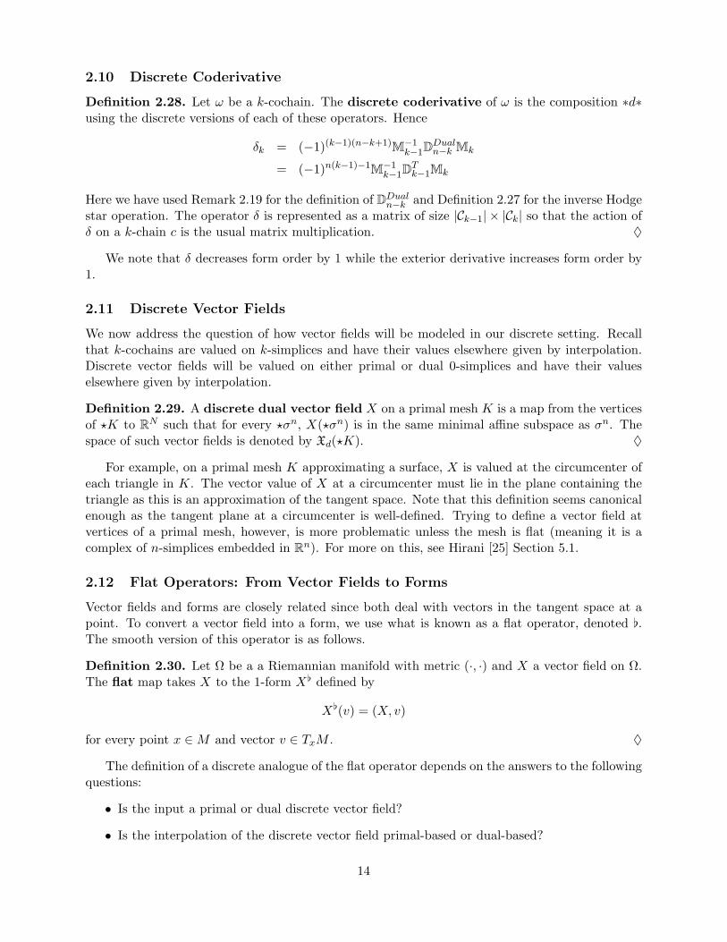
2.10 Discrete Coderivative
Definition 2.28. Let ω be a k-cochain. The discrete coderivative of ω is the composition ∗d∗using the discrete versions of each of these operators. Hence
δk = (−1)(k−1)(n−k+1)M−1k−1DDual
n−k Mk
= (−1)n(k−1)−1M−1k−1DT
k−1Mk
Here we have used Remark 2.19 for the definition of DDualn−k and Definition 2.27 for the inverse Hodge
star operation. The operator δ is represented as a matrix of size |Ck−1| × |Ck| so that the action ofδ on a k-chain c is the usual matrix multiplication. ♦
We note that δ decreases form order by 1 while the exterior derivative increases form order by1.
2.11 Discrete Vector Fields
We now address the question of how vector fields will be modeled in our discrete setting. Recallthat k-cochains are valued on k-simplices and have their values elsewhere given by interpolation.Discrete vector fields will be valued on either primal or dual 0-simplices and have their valueselsewhere given by interpolation.
Definition 2.29. A discrete dual vector field X on a primal mesh K is a map from the verticesof ?K to RN such that for every ?σn, X(?σn) is in the same minimal affine subspace as σn. Thespace of such vector fields is denoted by Xd(?K). ♦
For example, on a primal mesh K approximating a surface, X is valued at the circumcenter ofeach triangle in K. The vector value of X at a circumcenter must lie in the plane containing thetriangle as this is an approximation of the tangent space. Note that this definition seems canonicalenough as the tangent plane at a circumcenter is well-defined. Trying to define a vector field atvertices of a primal mesh, however, is more problematic unless the mesh is flat (meaning it is acomplex of n-simplices embedded in Rn). For more on this, see Hirani [25] Section 5.1.
2.12 Flat Operators: From Vector Fields to Forms
Vector fields and forms are closely related since both deal with vectors in the tangent space at apoint. To convert a vector field into a form, we use what is known as a flat operator, denoted [.The smooth version of this operator is as follows.
Definition 2.30. Let Ω be a a Riemannian manifold with metric (·, ·) and X a vector field on Ω.The flat map takes X to the 1-form X[ defined by
X[(v) = (X, v)
for every point x ∈M and vector v ∈ TxM . ♦
The definition of a discrete analogue of the flat operator depends on the answers to the followingquestions:
• Is the input a primal or dual discrete vector field?
• Is the interpolation of the discrete vector field primal-based or dual-based?
14
• Is the desired output a primal or dual discrete differential form?
These questions can be answered independently, meaning there are a total of 8 discrete flat oper-ators [25]. For now, we only define the discrete flat operator for dual vector fields, primal-basedinterpolation, and primal discrete differential forms. This operator is denoted [dpp and defined asfollows.
Definition 2.31. Let K be a primal mesh of dimension n and X ∈ Xd(?K) a dual discrete vectorfield on K. The discrete DPP-flat is a map [dpp : Xd(?K)→ C1(K) defined by its evaluation ofa primal 1-simplex σ1 as
< X[dpp , σ1 >=∑σnσ1
| ? σ1 ∩ σn|| ? σ1|
X(?σn) · ~σ1
where · is the usual dot product and ~σ1 indicates the vector with the same direction, length, andorientation as σ1. ♦
Thus, the flat operator [dpp assigns a value at σ1 based on the projection of X values at thecircumcenters of adjacent n-simplices, weighted by geometrical relevance. These weights may seemsomewhat arbitrary at the moment, however, they turn out to be the exact weights needed to createa discrete divergence theorem.
Definition 2.32. The discrete divergence divX of a discrete vector field X is defined to be
div(X) := −δ1X[ = −M−1
0 DT0 M1X
[
where [ is [dpp if X is a dual discrete vector field and [pdd if X is a primal discrete vector field. ♦
Lemma 2.33. Discrete Divergence Theorem on a Dual n-cell. (Hirani [25]) Let K be aprimal mesh of dimension n and σ0 a vertex in K. Let X ∈ Xd(?K) be a dual vector field. Then
| ? σ0| < div(X), σ0 >=∑σ1σ0
∑σnσ1
| ? σ1 ∩ σn|(X(?σn) · ~σ
1
|σ1|
)(8)
where the edges σ1 are oriented so that they all point outward.
Equation (8) says the divergence of X at σ0 is given by the flux of X through the boundary ofthe dual cell ?σ0. This suggests that the formal definition of discrete divergence (which dependedon our seemingly ad hoc choices for a discrete Hodge star and discrete flat operator) is in fact theexact definition required to capture the intuitive notion of divergence as a measurement of flux.This is emphasized further by the following Theorem and Corollary.
Theorem 2.34. Discrete Divergence Theorem on a Dual n-chain. (Hirani [25]) Let c bea dual n-chain which, as a set, is a simply connected subset of |K|. Then the discrete divergencetheorem is true over this set.
Corollary 2.35. Uniqueness of DPP-flat (Hirani [25]) The discrete divergence theorem on adual n-cell is true if and only if the coefficients in the DPP-flat definition, Definition 2.31, are
| ? σ1 ∩ σn|| ? σ1|
.
Similar results hold for primal complexes with the PDD-flat.
15
v2
v1
v0
bc
ic
cc
Figure 2: Reference for triangle notation.
2.13 Sample Calculation
To help illustrate how these operators are computed, we now explicitly state the discrete operatorsacting on a simple triangle in R2. Consider the triangle T in the xy plane with vertices v0, v1, andv2 at (0,0), (1,0), and (0,1), respectively, as shown for reference in Figure 2. We choose edges tobe oriented so that they point toward the vertex index of greater value and we assign the face acounterclockwise orientation.
First we compute the discrete exterior derivative operators as these are not geometry-dependent.
D0 =
−1 1 0−1 0 10 −1 1
, D1 =(
1 −1 1).
Now we turn to the Hodge star operator and begin first with a Hodge star defined directly viaa dual mesh. We run into an immediate problem as T is not well-centered (see Definition 2.10).Therefore, the dual mesh, as defined in this document, cannot be constructed. In an attempt toovercome this, we consider alternative centers for the triangle: the bartycenter (the average of thethree vertices) and the incenter (the center of the largest inscribed circle). These centers are:
circumcenter (cc) =(
12,12
), barycenter (bc) =
(13,13
), incenter (ic) =
(1
2 +√
2,
12 +√
2
).
For each center, we use the definition provided in Example 2.26 to compute the Hodge starmatrices M0 and M1 which act on discrete 0-forms and discrete 1-forms, respectively.
Mcc0 =
14 0 00 1
8 00 0 1
8
Mbc0 ≈
0.167 0 00 0.167 00 0 0.167
Mic0 ≈
0.146 0 00 0.177 00 0 0.177
Mcc1 =
12 0 00 1
2 00 0 0
Mbc1 ≈
0.373 0 00 0.373 00 0 0.167
Mic1 ≈
0.359 0 00 0.359 00 0 0.207
The circumcentric dual gives a non-invertible M1 matrix since the circumcenter lies on the edgefrom v1 to v2. The barycentric and incentric duals lie interior so they give diagonal matrices withpositive entries as desired.
To compute the coderivative, we use Definition 2.28 with n = 2 and k = 1. Hence δ1 =−M−1
0 DT0 M1 yielding
δcc1 =
2 2 0−4 0 0
0 −4 0
δbc1 ≈
2.236 2.236 0−2.236 0 1
0 −2.236 −1
δic1 ≈
2.449 2.449 0−2.029 0 1.172
0 −2.029 −1.172
16
It is evident from this example that the choice of “center” of a simplex has a significant effect onthe geometry-dependent operators computed to act on that simplex.
For comparison, we now consider the approach of computing a discrete Hodge star via Whitneyinterpolatory forms. This is the approach employed in the thesis of Nathan Bell [7]. The Whitney0-forms are the barycentric basis functions associated to the vertices of the triangle:
w0 = −x− y + 1w1 = x
w2 = y
The three Whitney 1-forms for this example correspond to the edges (v0, v1), (v0, v2) and (v1, v2):
w01 = w0∇w1 − w1∇w0 =< 1− y, x >w02 = w0∇w2 − w2∇w0 =< y, 1− x >w12 = w1∇w2 − w2∇w1 =< −y, x >
We check two basic properties of Whitney forms for w01. First, it should be identically 0 on verticesnot on edge (v0, v1) and indeed w01(v2) =< 0, 0 >. Second, it should have value 1 on the edge(v0, v1), meaning its dot product with a unit tangent vector in the direction of the edge shouldequal 1. A simple calculation confirms this. The analagous properties hold for the other 1-forms.For more on Whitney form calucation, see, for instance, Chapter 5 in Bossavit [12].
Let i and j index the set 01, 02, 12. The Hodge star is taken to be the mass matrix for thewi, namely:
MWhit1 := (< wi, wj >)ij =
(∫Twi · wjdA
)ij
=
13
16 0
16
13 0
0 0 16
The downside to this Hodge star is that it is not diagonal meaning it is more computatinallyexpensive to use, especially for problems involving very large meshes. The upshot is that thereis no need to choose or compute a dual mesh, thereby avoiding some potential numerical issues.Research on efficient and accurate Hodge stars is an ongoing challenge.
3 Darcy flow example
Recent work by Hirani et al. [26] uses a DEC method to model Darcy flow, a description of theflow of a viscous fluid in a permeable medium. We break down the problem using the three stepsoutlined in Section 1.2.
3.1 Step 1: Governing Equations
The first step is to fix the equations governing the phenomena in question and hence describe thePDE to be solved. Let Ω ⊂ Rn be a bounded open domain with piecewise smooth boundary ∂Ωand n = 2 or 3. The goal is to solve for the Darcy velocity v : Ω → Rn [30] and for the pressurep : Ω→ R. The governing equations under the assumption of no external body force are given by
v +k
µ∇p = 0 in Ω, (9)
divv = φ in Ω, (10)v · n = ψ on ∂Ω, (11)
17
where k > 0 is the coefficient of permeability, µ > 0 is the coefficient of viscosity, φ : Ω → R isthe prescribed divergence of velocity, and ψ : ∂Ω → R is the prescribed normal component of thevelocity across the boundary. The functions φ and ψ are given as input (sometimes called the loaddata) and it is assumed that
∫Ω φdΩ =
∫∂Ω ψdΓ.
3.2 Step 2: Domain, Variable, and Operator Replacement
The goal of this step is to write all the equations in terminology common to both smooth anddiscrete exterior calculus. First consider Equation (9), known as Darcy’s law. The pressure p isa scalar valued function so it is immediately a 0-form. The gradient operator ∇ becomes the 0thexterior derivative operator d0 in differential form language, meaning ∇p → d0p ∈ Λ1. Since v isbeing added to a 1-form, we must convert v from its vector field form to a 1-form, implying v → v[.The [ operator here is the smooth [ operator as defined in [1]. Our revised equation is then
v[ +k
µ(d0p) = 0.
Next, we turn to Equation (10), the continuity condition. We already know v → v[ and that thediv operator corresponds to dn−1. Since dn−1 must act on a (n−1)-form, we take the Hodge star ofv[, i.e. divv → dn−1(∗v[). This implies the right side of the equation must be made into an n-formalso which is accomplished by multiplying ω, the volume n-form on Ω, by the scalar data φ. Theresult is
dn−1(∗v[) = φω.
Finally, consider the boundary condition of Equation (11). The equation relates data on theboundary, i.e. information encoded in (n− 1)-forms. Let γ be the natural volume (n− 1)-form onthe boundary, defined by the condition
γ(X1, . . . , Xn−1) = ω(n,X1, . . . , Xn−1),
for all vector fields X1, . . . , Xn−1 on ∂Ω. Therefore, we will multiply ψ by γ for the right side of theequation. On the left side, v · n becomes ∗v[ by a converting from one notation to the other (formore on this see Abraham et al. [1] page 506). Thus, all three equations have now been re-writtenas
v[ +k
µ(d0p) = 0 in Ω, (12)
dn−1(∗v[) = φω in Ω, (13)
∗v[ = ψγ on ∂Ω. (14)
For convenience, we define the volumetric flux (if n = 3) or area flux (if n = 2) as
f := ∗(v[).
Taking ∗ of both sides of (12), we re-write the equations as
f +k
µ(∗d0p) = 0 in Ω, (15)
dn−1f = φω in Ω, (16)f = ψγ on ∂Ω. (17)
18
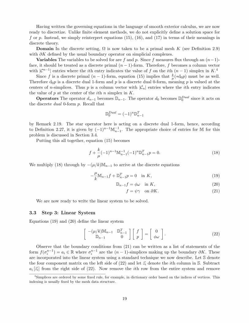
Having written the governing equations in the language of smooth exterior calculus, we are nowready to discretize. Unlike finite element methods, we do not explicitly define a solution space forf or p. Instead, we simply reinterpret equations (15), (16), and (17) in terms of their meanings indiscrete theory.
Domain In the discrete setting, Ω is now taken to be a primal mesh K (see Definition 2.9)with ∂K defined by the usual boundary operator on simplicial complexes.
Variables The variables to be solved for are f and p. Since f measures flux through an (n−1)-face, it should be treated as a discrete primal (n− 1)-form. Therefore, f becomes a column vectorwith |Cn−1| entries where the ith entry indicates the value of f on the ith (n− 1) simplex in K.4
Since f is a discrete primal (n − 1)-form, equation (15) implies that kµ(∗d0p) must be as well.
Therefore d0p is a discrete dual 1-form and p is a discrete dual 0-form, meaning p is valued at thecenters of n-simplices. Thus p is a column vector with |Cn| entries where the ith entry indicatesthe value of p at the center of the ith n simplex in K.
Operators The operator dn−1 becomes Dn−1. The operator d0 becomes DDual0 since it acts on
the discrete dual 0-form p. Recall that
DDual0 = (−1)nDT
n−1
by Remark 2.19. The star operator here is acting on a discrete dual 1-form, hence, accordingto Definition 2.27, it is given by (−1)n−1M−1
n−1. The appropriate choice of entries for M for thisproblem is discussed in Section 3.4.
Putting this all together, equation (15) becomes
f +k
µ(−1)n−1M−1
n−1(−1)nDTn−1p = 0. (18)
We multiply (18) through by −(µ/k)Mn−1 to arrive at the discrete equations
−µk
Mn−1f + DTn−1p = 0 in K, (19)
Dn−1f = φω in K, (20)f = ψγ on ∂K. (21)
We are now ready to write the linear system to be solved.
3.3 Step 3: Linear System
Equations (19) and (20) define the linear system[−(µ/k)Mn−1 DT
n−1
Dn−1 0
] [fp
]=[
0φω
]. (22)
Observe that the boundary conditions from (21) can be written as a list of statements of theform f(σn−1
i ) = ai ∈ R where σn−1i are the (n− 1)-simplices making up the boundary ∂K. These
are incorporated into the linear system using a standard technique we now describe. Let S denotethe four component matrix on the left side of (22) and let ~zi denote the ith column in S. Subtractai [~zi] from the right side of (22). Now remove the ith row from the entire system and remove
4Simplices are ordered by some fixed rule, for example, in dictionary order based on the indices of vertices. Thisindexing is usually fixed by the mesh data structure.
19
~zi from S. Repeating this process for each boundary constraint, we reduce the dimension of thesystem by exactly the number of boundary elements, as desired.
We now echo the authors’ observation that this matrix equation cleanly distinguishes the por-tions of the problem that are dependent on mesh connectivity (i.e. the blocks containing D matrices)and those that are dependent on the physical variable relations (i.e. the block containing the Mmatrix). Therefore, errors in physical measurements corrupt only a known part of the calculations.This is a useful property shared by some mixed finite element methods.
To implement this method, φ and ψ must be provided. Often φ is set to 0 to indicate thatdivv = 0 in Ω. Otherwise, φ may be set based on the solution to a known problem to test if themethod captures the correct solution. Specification of ψ is an assignment of values to boundary(n − 1)-simplices. The solver will then produce values of p at the center of each n-simplex andvalues of f at each edge.
For visualization and interpretation of the results, f is interpolated back to a smooth 1-formusing the Whitney interpolant. Values of the 1-form are computed at specified domain points(the authors use barycenters for convenience) and the corresponding vector field is deduced. Inparticular, if n = 2 and the 1-form value at a point is f = adx+ bdy with a and b constant, then
v[ = −(∗f) = − ∗ (adx+ bdy) = bdx− ady.
For the standard metric in R2, this means v is the vector (b,−a). If n = 3 and the 1-form value isf = ady ∧ dz + bdz ∧ dx+ cdx ∧ dy, then
For the standard metric in R3, this means v is the vector (a, b, c). The results of a number of testsof this system are shown in the paper [26].
3.4 Hodge Star for Darcy Flow
Darcy flow modeling allows for the medium to be non-homogeneous meaning there may be dif-ferent permeability constants in each n-dimensional simplex. Hence, the diagonal entry of Mn−1
corresponding to an (n − 1)-simplex σn−1 ought to be weighted with respect to the permeabilitycoefficients on either side of σn−1.
Here, the appropriate weights are determined by DEC theory in order to yield a discrete di-vergence theorem. Rather than take an arithmetic or geometric average, the weights are definedas follows. Let σn+ and σn− be the n-simplices containing σn−1 with permeabilities k+ and k−,respectively. Recall that ?σn−1 is the dual simplex to σn−1, i.e. an edge in the dual mesh. Theweight is then given by
| ? σn−1||σn−1|
| ? σn−1|k+| ? σn−1 ∩ σn+|+ k−| ? σn−1 ∩ σn−|
, (23)
where | · | represents the appropriate dimensional geometric measure. That this weighting schemeprovides for a discrete divergence theorem is shown in [25], Figure 5.4, Section 5.5, and Section 6.1.Note that whenever k+ = k−, (23) reduces to the general purpose Hodge star defined in Equation(7).
3.5 The importance of well-centerdness
The DEC analysis used to derive this method requires that the solution [f p]T provide values ofthe flux f on (n − 1)-simplices (i.e. edges in triangle meshes and triangles in tetrahedral meshes)
20
and values of the pressure p at the circumcenters of n-simplices. For the pressure values to haveany meaning, the mesh must be well-centered meaning the circumcenter of each simplex must lie inthe interior of the simplex (recall Definition 2.10). Since this criterion is often violated by meshingschemes (e.g. an obtuse triangle is not well-centered), pressure is assigned instead to the barycentersof n-simplices. The authors point out that the error introduced by this modification prevents theexact representation of linear variation of pressure over the domain (see Figure 3 in the paper). Ifthe mesh is well-centered, however, the DEC method gives excellent results (see Figures 10 and 11in the paper, for example).
3.6 Conclusion and Future Work
At the heart of the Darcy Flow example presented above as well as many other numerical methodslies a need for a “good” discrete Hodge star. Here, “good” means both faithfully representing theproperties of the smooth Hodge star at the discrete level and allowing for efficient computation viaa diagonal or sparse matrix formulation.
Currently, there are two main camps on how this could be accomplished. One approach is to useWhitney forms to construct the operator, possibly allowing for lumping of elements [7] or higherorder approximations [32]. The other approach is to try to construct well-centered dual meshes[33] and use barycentric duals when this is not possible. Auchmann and Kurz [4] attempt to bridgethe two options by evaluating Whitney forms at the barycenters of elements to construct a Hodgestar. Nonetheless, it is unlikely that there is a silver bullet solution to the problem as the needs ofan individual application dictate the relative importance of the various properties a discrete HodgeStar might have. Hiptmair provides a useful albeit theoretical overview to the problem in [24].
In addition to research on discrete Hodge star operators, much work remains to be done inDiscrete Exterior Calculus. On the theoretical side, other notions from smooth exterior calculusstill need to be transfered to the discrete setting such as Lie derivatives (as discussed in Hirani’sthesis [25]). On the computational side, few DEC-based solvers have been implemented and plentyremains to be studied regarding convergence and error analysis estimates. As a greater number ofPDE problems are considered in a DEC framework, further inquiries will undoubtedly arise.
References
[1] R. Abraham, J. E. Marsden, and T. Ratiu. Manifolds, tensor analysis, and applications,volume 75 of Applied Mathematical Sciences. Springer-Verlag, New York, second edition,1988.
[2] M. A. Armstrong. Basic topology. Springer-Verlag, New York, 1983.
[3] D. Arnold, R. Falk, and R. Winther. Finite element exterior calculus, homological techniques,and applications. Acta Numerica, pages 1–155, 2006.
[4] B. Auchmann and S. Kurz. A geometrically defined discrete hodge operator on simplicial cells.Magnetics, IEEE Transactions on, 42(4):643–646, 2006.
[5] I. Babuska and A. Aziz. Survey lectures on the mathematical foundations of the finite elementmethod. In The Mathematical Foundations of the FEM with Applications to PDEs, Proc.Sympos. Univ. Maryland; Academic Press, 1972.
[6] D. Baldomir. Differential forms and electromagnetism in 3-dimensional Euclidean space R3.Proc. IEE-A, 133(3):139–143, 1986.
21
[7] W. N. Bell. Algebraic multigrid for discrete differential forms (dissertation). Technical report,University of Illinois at Urbana-Champaign, 2008.
[8] P. Bochev and J. Hyman. Principles of mimetic discretizations of differential operators. InCompatible Spatial Discretizations, pages 89–119. Springer, 2006.
[9] A. Bossavit. Mixed finite elements and the complex of Whitney forms. In J. Whiteman, editor,The mathematics of finite elements and applications VI, pages 137–144. Academic Press, 1988.
[10] A. Bossavit. Whitney forms: a class of finite elements for three-dimensional computations inelectromagnetism. Proc. of the IEEE, 135(8):493–500, 1988.
[11] A. Bossavit. Differential Geometry for the Student of Numerical Methods in Electromagnetism.In preparation: http://butler.cc.tut.fi/ bossavit/Books/DGSNME/DGSNME.pdf, 1991.
[12] A. Bossavit. Computational Electromagnetism. Academic Press Inc., San Diego, CA, 1998.
[13] A. Bossavit. Computational electromagnetism and geometry (1)-(6). J. Japan Soc. Appl.Electroman. and Mech., 7–8:multiple articles, 2000.
[14] A. Bossavit. Generalized finite differences in computational electromagnetics. In F. Teixeira,editor, Progress in Electromagnetics Research, PIER 32, pages 45–64, 2001.
[15] S. Brenner and L. Scott. The Mathematical Theory of Finite Element Mehtods. Springer-Verlag, New York, 2002.
[16] P. Castillo, J. Koining, R. Rieben, M. Stowell, and D. White. Discrete differential forms:A novel methodology for robust computational electromagnetics. Technical report, LawrenceLivermore National Laboratory, Center for Applied Scientific Computing, 2003.
[17] M. Desbrun, A. N. Hirani, M. Leok, and J. E. Marsden. Discrete Exterior Calculus.arXiv:math/0508341, 2005.
[18] M. Desbrun, E. Kanso, and Y. Tong. Discrete differential forms for computational modeling.In SIGGRAPH ’06: ACM SIGGRAPH 2006 Courses, pages 39–54, New York, NY, USA,2006. ACM.
[19] G. Deschamps. Electromagnetics and differential forms. Proc. of the IEEE, 69(6):676–696,1981.
[20] J. Frauendiener. Discrete differential forms in general relativity. Classical and QuantumGravity, 23(16):S369–S385, 2006.
[21] D. Griffiths. Introduction to Electrodynamics. Prentice Hall, 1981.
[22] A. Hatcher. Algebraic topology. Cambridge University Press, Cambridge, 2002.
[23] R. Hiptmair. Canonical construction of finite elements. Mathematics of Computation,68(228):1325–1346, 1999.
[24] R. Hiptmair. Discrete hodge-operators: an algebraic perspective. Progress In ElectromagneticsResearch, 32:247–269, 2001.
[25] A. N. Hirani. Discrete exterior calculus (dissertation). Technical report, California Instituteof Technology, 2003.
22
[26] A. N. Hirani, K. B. Nakshatrala, and J. H. Chaudhry. Numerical method for Darcy flowderived using Discrete Exterior Calculus. arXiv:0810.3434, 2008.
[27] J. M. Hyman and M. Shashkov. Adjoint operators for the natural discretizations of the di-vergence gradient and curl on logically rectangular grids. Appl. Numer. Math., 25(4):413–442,1997.
[28] J. M. Hyman and M. Shashkov. Natural discretizations for the divergence, gradient, and curlon logically rectangular grids. Computers and Mathematics with Applications, 33(4):81 – 104,1997.
[29] J. M. Hyman and M. Shashkov. The orthogonal decomposition theorems for mimetic finitedifference methods. SIAM Journal on Numerical Analysis, 36(3):788–818, 1999.
[30] A. Masud and T. J. R. Hughes. A stabilized mixed finite element method for darcy flow.Computer Methods in Applied Mechanics and Engineering, 191(39-40):4341 – 4370, 2002.
[31] J. R. Munkres. Elements of algebraic topology. Addison-Wesley Publishing Company, MenloPark, CA, 1984.
[32] F. Rapetti. High order edge elements on simplicial meshes. ESAIM:M2AN, 41(6):1001–1020,2007.
[33] E. VanderZee, A. Hirani, D. Guoy, and E. Ramos. Well-centered triangulation. SIAM Journalon Scientific Computing, accepted 2008.
[34] M. Wardetzky, M. Bergou, D. Harmon, D. Zorin, and E. Grinspun. Discrete quadratic curva-ture energies. Comput. Aided Geom. Des., 24(8-9):499–518, 2007.
[35] H. Whitney. Geometric Integration Theory. Princeton University Press, 1957.
[36] A. Yavari. On geometric discretization of elasticity. Journal of Mathematical Physics,49(2):022901–1–36, 2008.