Notes on Fourier Series Steven A. Tretter October 30, 2013 Contents 1 The Real Form Fourier Series 3 2 The Complex Exponential Form of the Fourier Series 9 3 Fourier Series for Signals with Special Symmetries 13 3.1 Even Signals ............................ 13 3.2 Odd Signals ............................ 14 3.3 Half Wave Symmetry ....................... 14 4 Fourier Series for Some Simple Operations on Periodic Sig- nals 15 4.1 Linearity .............................. 15 4.2 The Delay Theorem ........................ 15 4.3 Differentiation ........................... 16 4.4 Integration ............................. 16 4.5 Multiplication of Two Periodic Signals with the Same Period . 19 4.6 Fourier Coefficients for the Complex Conjugate of a Signal .. 20 4.7 Average Power and Parseval’s Theorem ............. 20 5 Minimum Mean-Square Error Approximation 22 6 Fourier Series and LTI Systems 23 7 Speed of Convergence 25 1
Transcript
Notes on Fourier Series
Steven A. Tretter
October 30, 2013
Contents
1 The Real Form Fourier Series 3
2 The Complex Exponential Form of the Fourier Series 9
4 Fourier Series for Some Simple Operations on Periodic Sig-nals 154.1 Linearity . . . . . . . . . . . . . . . . . . . . . . . . . . . . . . 154.2 The Delay Theorem . . . . . . . . . . . . . . . . . . . . . . . . 154.3 Differentiation . . . . . . . . . . . . . . . . . . . . . . . . . . . 164.4 Integration . . . . . . . . . . . . . . . . . . . . . . . . . . . . . 164.5 Multiplication of Two Periodic Signals with the Same Period . 194.6 Fourier Coefficients for the Complex Conjugate of a Signal . . 204.7 Average Power and Parseval’s Theorem . . . . . . . . . . . . . 20
5 Minimum Mean-Square Error Approximation 22
6 Fourier Series and LTI Systems 23
7 Speed of Convergence 25
1
8 Effect of Truncating a Fourier Series by a Coefficient Win-dow 26
2
Let x(t) be a periodic signal with period T0 and fundamental frequency
ω0 = 2π/T0. Fourier showed that these signals can be represented by asum of scaled sines and cosines at multiples of the fundamental frequency.The series can also be expressed as sums of scaled complex exponentialsat multiples of the fundamental frequency. A sinusoid at frequency nω0 iscalled an nth harmonic. This document presents the approach I have takento Fourier series in my lectures for ENEE 322 Signal and System Theory.Unless stated otherwise, it will be assumed that x(t) is a real, not complex,signal. However, periodic complex signals can also be represented by Fourierseries.
1 The Real Form Fourier Series
as follows:
x(t) =a02
+∞∑
n=1
an cosnω0t+ bn sinnω0t (1)
This is called a trigonometric series. We will call it the real form of theFourier series.
To derive formulas for the Fourier coefficients, that is, the a′s and b′s,we need trigonometric identities for the products of cosines and sines. Youshould already know the following formulas for the cosine of the sum anddifference of two angles.
cos(a+ b) = cos a cos b− sin a sin b (2)
cos(a− b) = cos a cos b+ sin a sin b (3)
Adding these two equations and dividing by two gives
cos a cos b =1
2cos(a+ b) +
1
2cos(a− b) (4)
Subtracting the second equation from the first and dividing by 2 gives
sin a sin b =1
2cos(a− b)− 1
2cos(a+ b) (5)
You should already know the following two trigonometric identities:
sin(a+ b) = sin a cos b+ cos a sin b (6)
3
sin(a− b) = sin a cos b− cos a sin b (7)
Adding these last two equations give
sin a cos b =1
2sin(a+ b) +
1
2sin(a− b) (8)
To find a0/2 consider the integral of x(t) over one complete period T0.For some conveniently chosen starting time t0 this is
t0+T0∫
t0
x(t) dt = T0a02
+∞∑
n=1
an
t0+T0∫
t0
cosnω0t dt+ bn
t0+T0∫
t0
sinnω0t dt (9)
Each integral in the sum is over n complete periods of a sine or cosine andis zero. Therefore
a02
=1
T0
t0+T0∫
t0
x(t) dt (10)
which is just the DC value of x(t).To find an for n ≥ 1 consider the following integral for k ≥ 1:
t0+T0∫
t0
x(t) cos kω0t dt =
t0+T0∫
t0
a02cos kω0t dt+
∞∑
n=1
an
t0+T0∫
t0
cosnω0t cos kω0t dt
+ bn
t0+T0∫
t0
sinnω0t cos kω0t dt (11)
Using identity (4) gives
t0+T0∫
t0
cosnω0t cos kω0t dt =1
2
t0+T0∫
t0
cos[(n−k)ω0t] dt+1
2
t0+T0∫
t0
cos[(n+k)ω0t] dt
(12)The first integral on the right-hand-side is over |n − k| complete periods ofthe cosine and is zero when n 6= k and T0/2 when n = k. The second integral
4
is over n+ k periods and is always zero. Using identity (8) gives
t0+T0∫
t0
sinnω0t cos kω0t dt =1
2
t0+T0∫
t0
sin[(n+ k)ω0t] dt+1
2
t0+T0∫
t0
sin[(n− k)ω0t] dt
(13)The two integrals on the right are zero even when n = k. Therefore
an =2
T0
t0+T0∫
t0
x(t) cosnω0t dt for n ≥ 1 (14)
To find bn for n ≥ 1 consider the following integral for k ≥ 1:
t0+T0∫
t0
x(t) sin kω0t dt =
t0+T0∫
t0
a02sin kω0t dt+
∞∑
n=1
an
t0+T0∫
t0
cosnω0t sin kω0t dt
+ bn
t0+T0∫
t0
sinnω0t sin kω0t dt (15)
Using identity (8) gives
t0+T0∫
t0
cosnω0t sin kω0t dt =1
2
t0+T0∫
t0
sin[(k+n)ω0t] dt+1
2
t0+T0∫
t0
sin[(k−n)ω0t] dt
(16)The first integral on the right-hand-side is over k+n complete periods of thesine and is always zero. The second integral is over |k − n| periods and isalways zero also. Using identity (5) gives
t0+T0∫
t0
sinnω0t sin kω0t dt =1
2
t0+T0∫
t0
cos[(n−k)ω0t] dt−1
2
t0+T0∫
t0
cos[(n+k)ω0t] dt
(17)Both integrals on the right-hand-side are zero except when n = k. Then thefirst integral is T0/2. Therefore
bn =2
T0
t0+T0∫
t0
x(t) sinnω0t dt for n ≥ 1 (18)
5
The dot product of the three dimensional vectors A = axi + ayj + azkand B = bxi + byj + bzk is A · B = axbx + ayby + azbz. Give two functionsx(t) and y(t), the integral
t0+T0∫
t0
x(t)y(t) dt
is abstractly similar to the dot product. Two vectors are orthogonal if theirdot product is zero. It was shown above that the integrals of cosnω0t cos kω0tand sinnω0t sin kω0t over an interval of length T0 are always zero for k 6= n.Also the integral of sinnω0t cos kω0t over an interval of length T0 is zerofor all n and k Therefore, these sines and cosines can be considered to beorthogonal basis vectors in an infinite dimensional vector space. The Fouriercoefficients are the coordinates of the function x(t) with respect to the basisvectors in this infinite dimensional space.
Even though we have derived formulas for the an’s and bn’s this does notprove that the series converges to x(t) because the sines and cosines maynot be a rich enough set of functions. Fortunately, it can be shown that arather mild set of conditions know as the Dirichlet conditions guarantee theseries converges point wise to the function except at discontinuities. All thereal-world functions we encounter satisfy these conditions. See Oppenheimand Willsky1 for these conditions. Also, if the magnitude squared of x(t)integrated over one fundamental period is finite, it can be shown that theseries converges to x(t) in the sense that the integral over one fundamentalperiod of the squared magnitude of the error between x(t) and the series isconverges to zero. This is known as convergence in the mean-square errorsense.
Even if a function is not periodic, the Fourier series will converge tothe function over the interval of integration (t0, t0 + T0) and will extendperiodically outside this interval.
EXAMPLE 1 Symmetric Square Wave
Let x(t) be the symmetric square wave show by the dashed purple lines inFigure 1. The formula for one period of this square wave centered about the
1A.V. Oppenheim and A.S. Willsky, Signals and Systems, 2nd Edition, Prentice Hall,1996, pp. 197–198.
6
origin is
x(t) =
{
−A for − T0/2 < t < 0A for 0 < t < T0/2
(19)
The average or DC value of this signal is
a02
=1
T0
T0/2∫
−T0/2
x(t) dt = 0 (20)
For n ≥ 1
an =2
T0
T0/2∫
−T0/2
x(t) cosnω0t dt = 0 for n ≥ 1 (21)
This is true because function x(t) is odd and cosnω0 is even, so the productx(t) cosnω0t is odd and the integral of this product symmetrically about theorigin is zero. Using the facts that ω0T0 = 2π and x(t) and sinnω0t are bothodd so that their product is even, the coefficients of the sine terms are
bn =2
T0
T0/2∫
−T0/2
x(t) sinnω0t dt =4
T0
T0/2∫
0
x(t) sinnω0t dt =4
T0
T0/2∫
0
A sinnω0t dt
=4A
T0
[− cosnω0t
nω0
]∣
∣
∣
∣
T0/2
0
=2A
nπ(1− cosnπ) =
2A
nπ[1− (−1)n]
=
4A
nπfor n odd
0 for n even(22)
Using these coefficients, the Fourier series for the square wave can be writtenas
x(t) =4A
π
∞∑
n=1
1
2n− 1sin(2n− 1)ω0t (23)
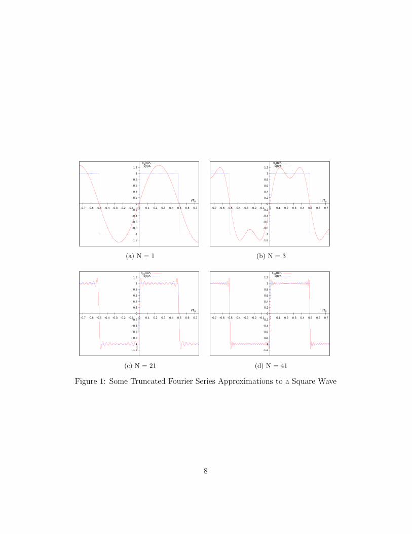
Approximations to x(t) when the sum is truncated at the N = 2n − 1harmonic or n = (N + 1)/2 for N = 1, 3, 21 and 41 are shown in Figure 1.Notice that there is a significant overshoot at a jump even as N becomeslarger. It can be shown that the jump remains at close to 9% of the heightof the jump as N increases. This is known as Gibbs’ phenomenon. The
Figure 1: Some Truncated Fourier Series Approximations to a Square Wave
8
frequency of the ripples increases but the ripples move closer to the jumpand decay more quickly away from the jump as N increases.
We saw in class that
a cos θ + b sin θ =√a2 + b2 cos[θ − arctan(b/a)] (24)
Therefore, the Fourier series can also be expressed as
x(t) =a02
+∞∑
n=1
√
a2n + b2n cos[nω0t− arctan(bn/an)] (25)
This form shows the amplitude and phase shift of each harmonic.
2 The Complex Exponential Form of the Fourier
Series
We will now see that the real form of the Fourier series can be convertedinto a more compact form that is a sum of scaled complex exponentials atmultiples of the fundamental frequency. Remember that
cos θ =ejθ + e−jθ
2and sin θ =
ejθ − e−jθ
2j(26)
Using these identities, the real form Fourier series becomes
x(t) =a02
+∞∑
n=1
anejnω0t + e−jnω0t
2+ bn
ejnωot − ejnω0t
2(27)
The series can be rearranged by collecting the terms involving ejnω0t ande−jnω0t resulting in
x(t) =a02
+∞∑
n=1
an − jbn2
ejnω0t +an + jbn
2e−jnω0t (28)
Now define the new coefficient cn as
cn =an − jbn
2=
1
T0
t0+T0∫
t0
x(t)(cosnω0t− j sinnω0t) dt
9
=1
T0
t0+T0∫
t0
x(t)e−jnω0t dt (29)
Notice that
an + jbn2
=1
T0
t0+T0∫
t0
x(t)ejnω0t dt = c−n anda02
= c0 (30)
Therefore (28) can be collapsed into the following single sum:
x(t) =∞∑
n=−∞
cnejnω0t (31)
where
cn =1
T0
t0+T0∫
t0
x(t)e−jnω0t dt (32)
It is interesting to observe that the complex exponentials in the series areorthogonal, that is,
1
T0
t0+T0∫
t0
ejnω0te−jmω0t dt =1
T0
t0+T0∫
t0
ej(n−m)ω0t dt =
{
1 for n = m0 for n 6= m
(33)
Therefore, the Fourier series can be thought of as the representation of x(t) inan infinite dimensional vector space where the basis vectors are the complexexponentials and the coordinates are the cn Fourier coefficients.
The coefficients of the real form of the series can be found from thecoefficients of the complex form by adding and subtracting cn and c−n to get
an = cn + c−n and jbn = c−n − cn (34)
If x(t) is real, then cn = c−n. In polar form cn = |cn|ejθn so c−n =|cn|e−jθn . The Fourier series then can be written as
x(t) = c0+∞∑
n=1
|cn|(
ej(nω0t+θn) + e−j(nω0t+θn))
= c0+∞∑
n=1
(2|cn|) cos(nω0t+ θn)
(35)By comparison with the real form of the series or by direct computation, itfollows that 2|cn| = (a2n + b2n)
1/2 and θn = − arctan(bn/an).
10
EXAMPLE 2 Pulse Train
One period of a periodic pulse train, x(t), is shown in Figure 2. The coeffi-
t
A
−T0
2τ
2T0
2−τ
2
x(t)
Figure 2: A Periodic Pulse Train
cients for the complex exponential form of the Fourier series are
xn =1
T0
τ/2∫
−τ/2
Ae−jnω0t dt =A
T0
τ/2∫
−τ/2
cosnω0t− j sinnω0t dt (36)
The integral of sinnω0 symmetrically about the origin is zero. The functioncosnω0t is even. Using these two facts gives
xn =2A
T0
τ/2∫
0
cosnω0t dt =2A
T0nω0
sinnω0τ/2 = Aτ
T0
sinnπ τT0
nπ τT0
(37)
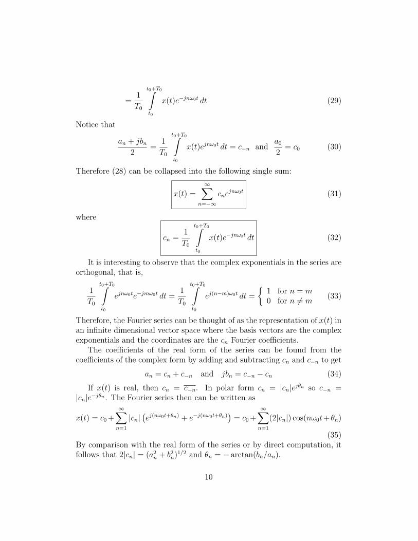
The quotient τ/T0 is called the duty factor of the pulse train. The fun-damental frequency for the pulse train is f0 = 1/T0. The frequency corre-sponding to coefficient xn is n/T0 = nf0. If nf0 is replaced by f in (37),the nulls of sin πτf occur when πτf = kπ or f = k/τ where k is an integer.The first null occurs at 1/τ which is the reciprocal of the pulse width. Usingthe original integral with n = 0 or by using L’Hospital’s rule it follows thatx0 = Aτ/T0 so the DC value is the pulse amplitude multiplied by the dutyfactor. The function
Figure 3: Magnitudes of the Fourier Coefficients for the Pulse Train withτ/T0 = 0.375.
is plotted in Figure 3 as the purple dashed line for τ/T0 = 0.375 or, equiva-lently, τ = 0.375/f0. Then the nulls occur at k/τ = kf0/0.375. The Fouriercoefficients xn/A are samples of g(f) for f = nf0. Some of the magnitudesof these coefficients are plotted as the vertical lines in Figure 3.
If T0 is fixed and τ decreases, the null at 1/τ increases. So, as intuitivelyexpected, the signal bandwidth increases as the pulse becomes shorter. Onthe other hand, when τ is fixed and T0 increases (or the fundamental fre-quency f0 decreases), the harmonic frequencies become closer together. Wewill see soon that when T0 becomes infinite so that x(t) is a single isolatedpulse at the origin, the plot of the coefficients becomes a continuum which iscalled the Fourier transform of the signal.
EXAMPLE 3 Period Train of Impulse Functions
Let x(t) =∑∞
n=−∞ δ(t − nT0). The complex exponential Fourier series
12
coefficients are
xn =1
T0
T0/2∫
T0/2
δ(t)e−jnω0t dt =1
T0
for all n (39)
Therefore
x(t) =1
T0
∞∑
n=−∞
ejnω0t (40)
The Fourier coefficients for this signal all have the same value 1/T0, so itsbandwidth is infinite.
3 Fourier Series for Signals with Special Sym-
metries
3.1 Even Signals
An even signal has the property that x(t) = x(−t) for all t. Remember thatthe coefficients of the cosine terms for the real form of the series are
an =2
T0
T0/2∫
−T0/2
x(t) cosnω0t dt (41)
The product x(t) cosnω0t is even since both factors are even. Therefore thesecoefficients can also be computed as
an =4
T0
T0/2∫
0
x(t) cosnω0t dt (42)
The formula for the coefficients of the sine terms is
bn =2
T0
T0/2∫
−T0/2
x(t) sinnω0t dt (43)
13
The product x(t) sinnω0t is odd since x(t) is even and sinnω0t is odd. There-fore the integral of this product symmetrically about the origin must be zeroand bn = 0 for all n. Thus the Fourier series is just a sum of cosine termsplus the DC value. These terms are all even functions. An even functioncannot contain any odd components, so no sine terms can be present.
The Fourier coefficients for the complex exponential form of the series are
cn = an/2 =2
T0
T0/2∫
0
x(t) cosnω0t dt (44)
because bn = 0. When x(t) is real, cn is real. For real or complex signalscn = c−n.
3.2 Odd Signals
3.3 Half Wave Symmetry
A signal x(t) has half wave symmetry if x(t + T0
2) = −x(t) for all t. The
symmetric square wave is an example of a signal with half wave symmetry.It will now be shown that signals of this type only have odd harmonics. TheFourier coefficients are
xn =1
T0
T0∫
0
x(t)e−jnω0t dt =1
T0
T0/2∫
0
x(t)e−jnω0t dt+1
T0
T0∫
T0/2
x(t)e−jnω0t dt
=1
T0
T0/2∫
0
x(t)e−jnω0t dt+1
T0
T0/2∫
0
x
(
t+T0
2
)
e−jnω0(t+T0
2) dt
=1
T0
T0/2∫
0
x(t)e−jnω0t + x
(
t+T0
2
)
e−jnω0te−jnω0T0/2 dt
=1
T0
T0/2∫
0
x(t)(
1− e−jnω0T0/2)
e−jnω0t dt =1
T0
T0/2∫
0
x(t)[
1− e−jnπ]
e−jnω0t dt
=1
T0
T0/2∫
0
x(t) [1− (−1)n] e−jnω0t dt
14
=
2
T0
T0/2∫
0
x(t)e−jnω0t dt for n odd
0 for n even
(45)
4 Fourier Series for Some Simple Operations
on Periodic Signals
4.1 Linearity
Let x(t) and y(t) be periodic signals each with period T0 and complex ex-ponential Fourier series coefficients xn and yn, respectively. Let z(t) =c1x(t) + c2y(t). Then by the linearity of integrals it follows that the Fouriercoefficients for z(t) are zn = c1xn + c2yn.
4.2 The Delay Theorem
Let the periodic signal x(t) with period T0 have the Fourier series expansion
x(t) =∞∑
n=−∞
xnejnω0t
Then the delayed signal y(t) = x(t− d) is
y(t) = x(t− d) =∞∑
n=−∞
xnejnω0(t−d) =
∞∑
n=−∞
(
xne−jnω0d
)
ejnω0t (46)
Thus the Fourier coefficients for y(t) are
yn = xne−jnω0d (47)
Notice that |yn| = |xn| but the delay adds a phase shift of −nωod to thecoefficients of x(t). This phase shift varies linearly with the frequency nω0.
15
4.3 Differentiation
Let x(t) be a periodic signal with period T0 and complex exponential Fourierseries coefficients xn. Then its derivative with respect to time is
y(t) =d
dtx(t) =
d
dt
∞∑
n=−∞
xnejnω0t =
∞∑
n=−∞
(jnω0xn)ejnω0t (48)
Therefore, the coefficients for the derivative are
yn = jnω0xn (49)
Notice that differentiation removes the DC value since y0 = 0. It emphasizesthe high frequency harmonics by a factor increasing linearly with the har-monic frequency nω0. In addition, the factor j adds a 90 degree phase shiftto each component.
4.4 Integration
Let x(t) be a periodic signal with period T0, Fourier coefficients xn, andaverage value x0 = 0. Consider the signal
y(t) =
t∫
−∞
x(τ) dτ (50)
If x0 were not zero then this integral would increase with t without boundand y(t) would not be periodic. Integrating the complex exponential Fourierseries for x(t) gives
y(t) =∞∑
n=−∞n 6=0
xn
jnω0
ejnω0τ dτ +K (51)
where K is a constant of integration. Since the sum does not contain then = 0 term, K must be the average value y0 of y(t). From the sum it is clearthat the Fourier coefficients of y(t) are
yn =xn
jnω0
for n 6= 0 and y0 = average value of y(t) (52)
16
Integration emphasizes the low frequency components and attenuates thehigh frequency ones by a factor inversely proportional to frequency. The 1/jterm adds a −90 degree phase shift to each harmonic.
EXAMPLE 4 Fourier Series for a Triangular Wave
The differentiation and integration theorems along with the train of impulses
−T0
2T0
2
��
��@
@@@�
��
?
6
?
66
?
6
A
t
2AT0
t0
−2AT0
x(t)
x(t)
t
4AT0
−4AT0
T0
2−T0
23T0
2−3T0
2
−3T0
2−3T0
2
x(t)
@@
@@
0
��
��@
@@
@��
��@
@
Figure 4: Triangular Wave
example can be used to easily find the Fourier series for signals consisting of
17
polynomial segments. The method is to differentiate the signal repeatedlyuntil a sum of impulse trains arises. The Fourier series for this sum of impulsetrains is easily found from the single impulse train example and the delaytheorem. The resulting coefficients are then divided by jnω0 raised to thenumber of derivatives used to get to the sum of impulse trains. Finally, then = 0 coefficient must be set equal to the average value of the original signal.To illustrate this procedure consider the triangular wave shown in Figure 4.An equation for x(t) is
x(t) = −4A
T0
∞∑
n=−∞
δ(t− nT0) +4A
T0
∞∑
n=−∞
δ
(
t− nT0 −T0
2
)
(53)
Notice that the second sum on the right hand side is the first sum delayedby T0/2 and with a sign change. Using the delay theorem and the result ofExample 3, the Fourier series coefficients for x(t) are x0 = 0 since its averageis zero and
xn = −4A
T0
(
1
T0
− 1
T0
e−jnω0T0/2
)
= −4A
T 20
[1− (−1)n] for n 6= 0 (54)
(The double dots above the coefficients do not mean “take the second deriva-tive of the coefficient.” They are an abuse of notation and simply indicatethat the coefficients are for the second derivative of x(t).) The average valueof x(t) is zero, so its Fourier coefficients are x0 = 0 and
xn =xn
jmω0
=
−4A
T 20
[1− (−1)n]
jnω0
for n 6= 0 (55)
The average value of x(t) is
x0 =1
T0
T0/2∫
−T0/2
x(t) dt =A
2(56)
and the coefficients for n > 0 are
xn =xn
(jnω0)2=
−4A[1− (−1)n]
(jnω0T0)2=
A[1− (−1)2]
(nπ)2for n 6= 0 (57)
18
More explicitly
xn =
A/2 for n = 0
0 for n even
2A
n2π2for n odd
(58)
If the average value A/2 is subtracted from x(t) the resulting signal is a trian-gular wave centered about the x-axis and has half wave symmetry. Thereforeit would be expected that the even harmonics are all zero except for the DCterm. The triangular wave is smoother than the symmetric square wave, soits Fourier coefficients decay faster, like 1/n2 rather than 1/n.
4.5 Multiplication of Two Periodic Signals with theSame Period
Let x(t) and y(t) be two signals with the same period and Fourier series
x(t) =∞∑
n=−∞
xnejnω0t y(t) =
∞∑
n=−∞
ynejnω0t
The product of these signals z(t) = x(t)y(t) has the Fourier coefficients
zn =∞∑
k=−∞
xkyn−k = xn ∗ yn (59)
It is interesting to see that discrete-time convolution arises in situations otherthan finding the output of a discrete-time LTI system by convolving the in-put with the impulse response.
Proof:The product can be written as
z(t) = x(t)y(t) =∞∑
k=−∞
xkejkω0ty(t) (60)
so the Fourier coefficients for z(t) are
zn =1
T0
t0+T0∫
t0
x(t)y(t)e−jnω0t dt =1
T0
t0+T0∫
t0
∞∑
k=−∞
xkejkω0ty(t)e−jnω0t dt
19
=∞∑
k=−∞
xk1
T0
t0+T0∫
t0
y(t)e−j(n−k)ω0t dt =∞∑
k=−∞
xkyn−k (61)
4.6 Fourier Coefficients for the Complex Conjugate ofa Signal
Let x(t) be a signal with the Fourier coefficients xn. Let y(t) = x(t). Theformula for computing xn is
xn =1
T0
t0+T0∫
t0
x(t)e−jnω0t dt (62)
Using the facts that the conjugate of an integral is the integral of the conju-gate of the integrand, and the conjugate of a product is the product of theconjugates of the factors gives
xn =1
T0
t0+T0∫
t0
x(t)ejnω0t dt so x−n =1
T0
t0+T0∫
t0
x(t)e−jnω0t dt (63)
Therefore, the Fourier coefficients for y(t) = x(t) are
yn = x−n (64)
In words, conjugation turns the spectrum around backwards and conjugatesthe terms.
4.7 Average Power and Parseval’s Theorem
The average power for a periodic signal x(t) with period T0 and Fouriercoefficients xn is
P =1
T0
t0+T0∫
t0
|x(t)|2 dt = 1
T0
t0+T0∫
t0
x(t)x(t) dt (65)
20
In (61) let y(t) = x(t), so yk = x−k and y−k = xk. Also let n = 0. Then (61)becomes
z0 =1
T0
t0+T0∫
t0
|x(t)|2 dt =∞∑
k=−∞
|xk|2 = P (66)
This is often referred to as Parseval’s Theorem. Using the same approach, itis easy to show that the cross-correlation between two sequences is
1
T0
t0+T0∫
t0
x(t)y(t) dt =∞∑
k=−∞
xkyk (67)
Let an and bn be the Fourier coefficients for the real form series andassume that x(t) is a real signal. Remember that
xn =an − jbn
2and x−n = xn
so that
|xn|2 = |x−n|2 =a2n + b2n
4(68)
Then
P =−1∑
n=−∞
|xn|2 + x20 +
∞∑
n=1
|xn|2 = x20 + 2
∞∑
n=1
|xn|2
=(a02
)2
+∞∑
n=1
a2n + b2n2
(69)
Remember that the amplitude of the nth harmonic in the real form series is√
a2n + b2n. Therefore the power associated with that harmonic is (a2n+b2n)/2.In summary, the total power in a periodic signal is the sum of the powers
of the individual harmonics. There are no cross terms between differentharmonics.
21
5 Minimum Mean-Square Error Approxima-
tion
Let x(t) be a periodic signal with the complex exponential Fourier series
x(t) =∞∑
n=−∞
xnejnω0t
Suppose we want to best approximate x(t) by a finite term trigonometricsum of the form
xN(t) =N∑
n=−N
αnejnω0t (70)
To proceed we must define what we mean by “best.” There are many choicesfor “best.” We will define “best” as selecting the coefficients {αn} to minimizethe average of the integral of the magnitude squared of the error between x(t)and xN(t) over one period. This is called the mean-square error or MSE. Wecould simply truncate the Fourier series for x(t) and choose the αn’s as theFourier coefficients, but is that the best choice? The instantaneous error is
ǫ(t) = x(t)− xN(t) =∞∑
n=−∞
xnejnω0t −
N∑
n=−N
αnejnω0t
=N∑
n=−N
(xn − αn)ejnω0t +
∑
|n|>N
xnejnω0t (71)
Thus ǫ(t) is a Fourier series with coefficients ǫn = xn − αn for −N ≤ n ≤ Nand xn for |n| > N . According to Parseval’s theorem, the MSE is
E2 =1
T0
t0+T0∫
t0
| ǫ(t)|2 dt =N∑
n=−N
|xn − αn|2 +∑
|n|>N
|xn|2 (72)
The coefficients xn are determined by the Fourier series for x(t). They arefixed and we cannot change them. Therefore, E2 is minimized by selectingαn = xn for −N ≤ n ≤ N . Thus the best choice for the αn’s is always theFourier coefficients xn for −N ≤ n ≤ N for every value of the truncation
22
limit N . With this choice, the minimum MSE is
min{αn}
E2 =∑
|n|>N
|xn|2 =∞∑
n=−∞
|xn|2 −N∑
n=−N
|xn|2
and by using Parseval’s theorem for the first integral on the right
=1
T0
t0+T0∫
t0
|x(t)|2 dt−N∑
n=−N
|xn|2 (73)
The integral of |x(t)|2 can be directly computed from the given x(t). A desiredMSE can be achieved by increasing N and incrementing the sum of |xn|2 untilthe desired value is reached. It is interesting to observe that increasing Ndoes not change the best coefficients found for smaller N . They are alwaysthe Fourier series coefficients. Another observation is that minimum MSE,(73), decreases to zero as N increases as a result of Parseval’s theorem.
EXAMPLE 5 Pulse Train (continued)
Consider the periodic pulse train of Example 2. By direct calculation usingx(t) and then Parseval’s theorem
1
T0
T0/2∫
−T0/2
|x(t)|2 dt = A2 τ
T0
=∞∑
n=−∞
A
τ
T0
sinnπτ
T0
nπτ
T0
2
(74)
The sum of squared Fourier coefficients can be truncated at increasing N tofind the value of N for a desired MSE.
6 Fourier Series and LTI Systems
Consider an LTI system with the impulse response h(t). If the input is thesinusoid x(t) = Cej(ωt+β) the output is
y(t) =
∞∫
−∞
h(τ)Cej[ω(t−τ)+β] dτ = Cej(ωt+β)
∞∫
−∞
h(τ)e−jωτ dτ = Cej(ωt+β)H(ω)
(75)
23
where on renaming τ to t
H(ω) =
∞∫
−∞
h(t)e−jωt dt (76)
The function H(ω) is called the frequency response of the system. Shortlywe will see that H(ω) is the Fourier transform of the impulse response. Thusthe output is a sinusoid at the same frequency as the input but scaled by thecomplex number H(ω). In polar form H(ω) = A(ω)ejθ(ω) where
A(ω) = |H(ω)| and θ(ω) = argH(ω) (77)
The function A(ω) is called the amplitude response of the system and θ(ω)is called the phase response of the system. The amplitude response in dB isα(ω) = 20 log10 A(ω). Thus the output can be written as
Thus when the input to a system is a sinusoid at some frequency, the out-put is a sinusoid at the same frequency but the amplitude is scaled by theamplitude response and the phase is shifted by the phase response of thesystem. Sinusoids are called the eigenfunctions of LTI systems in analogy tothe eigenvectors of a square matrix.
Both convolutions on the right hand side result in real signals. Therefore,comparing (78) and (79) we see that the output resulting from the inputC cos(ωt+ β) is
Thus for a real impulse response and input sine wave at frequency ω, theoutput is again a real sine wave at frequency ω scaled in amplitude by A(ω)and phase shifted by θ(ω).
24
If the input to an LTI system with impulse response h(t) is a periodicsignal x(t) with the Fourier series x(t) =
∑∞−∞ xne
jnω0t, then by superpositionthe output will be
y(t) =∞∑
n=−∞
H(nω0)xnejnω0t (81)
EXAMPLE 6
Consider a system with the impulse response h(t) = e−atu(t) with a > 0.The frequency response is
H(ω) =
∞∫
0
e−ate−jωt dt =1
jω + a(82)
The amplitude and phase responses are
A(ω) = |H(ω)| = 1√ω2 + a2
and θ(ω) = argH(ω) = − arctan(ω/a) (83)
This is an elementary lowpass filter. The amplitude response has a maximumat ω = 0 and decreases monotonically as |ω| increases. The output when theinput is a periodic signal with complex exponential Fourier series coefficients{xn} is
y(t) =∞∑
n=−∞
1
jnω0 + axne
jnω0t =∞∑
n=−∞
1√
(nω0)2 + a2xne
j[nω0t+θ(nω0)] (84)
7 Speed of Convergence
Some idea about the speed of convergence of Fourier series can be obtainedby assuming the signal consists of polynomial segment. Suppose x(t) mustbe differentiated K times until impulse trains first appear. We have seenthat the Fourier coefficients for an impulse train are all the same constant.The integration theorem states that the Fourier coefficients of x(t) are thoseof the Kth derivative divided by (jnω0)
K except for x0 which is the average
25
value of x(t). Therefore, the Fourier coefficients of x(t) decrease like 1/nK .The more derivatives required to get to impulses, the faster the Fourier coef-ficients decrease with n. The signal x(t) must be smoother when K is larger.This agrees with our intuition that smoother signals have less high frequencycontent.
8 Effect of Truncating a Fourier Series by a
Coefficient Window
Let x(t) be a periodic signal with the complex exponential Fourier seriescoefficients xn. A periodic signal y(t) is formed with the Fourier coefficientsyn = xnbn for some desired sequence bn. Typically, bn = 0 for |n| > N andtruncates the Fourier series. The sequence bn is called a coefficient window
and forming the product is called coefficient windowing. Let the artificialperiodic time signal formed from bn be
b(t) =∞∑
n=−∞
bnejnω0t (85)
The series for y(t) is
y(t) =∞∑
n=−∞
xnbnejnω0t (86)
Replacing xn by the integral to compute it gives
y(t) =∞∑
n=−∞
1
T0
t0+T0∫
t0
x(τ)e−jnω0τ dτ bnejnω0t
=1
T0
t0+T0∫
t0
x(τ)∞∑
n=−∞
bnejnω0(t−τ) dτ =
1
T0
t0+T0∫
t0
x(τ)b(t− τ) dτ (87)
The resulting integral is called the periodic convolution of x(t) and b(t).
EXAMPLE 7 Rectangular Window
As usual, let x(t) =∑∞
n=−∞ xnejnω0t. Let bn = 1 for −L ≤ n ≤ L and 0 for
26
n > |L|. The windowed signal is
y(t) =∞∑
n=−∞
xnbnejnω0t =
L∑
n=−L
xnejnω0t (88)
which is just the original series truncated below −L and above L. There areN = 2L+ 1 terms in the truncated series. The window time function is
b(t) =L∑
n=−L
ejnω0t = e−jLω0t(1 + ejω0t + · · ·+ ej2Lω0t) (89)
Using the formula for the sum of a geometric series we find that
b(t) = e−jLω0tej(2L+1)ω0t − 1
ejω0t − 1(90)
Factoring ej(2L+1)ω0t/2 from the numerator and ejω0t/2 from the denominatorand dividing both by 2j gives
b(t) = e−jLω0tej(2L+1)ω0t/2
ejω0t/2
(
ej(2L+1)ω0t/2 − e−j(2L+1)ω0t/2)
/(2j)
(ejω0t/2 − e−jω0t/2) /(2j)
=sinNω0t/2
sinω0t/2where N = 2L+ 1 (91)
From the original sum, (89), or by L’Hospital’s rule we see that b(0) = N .It has period T0 so b(kT0) = N for any integer k. The numerator has zerosat Nω0t/2 = mπ for integer m or at t = m2π/(Nω0) = mT0/N . Thusb(mT0/N) = 0 except when m is a multiple of N where it has a peak of valueN .
The area under b(t)/T0 over the interval −T0/2 < t < T0/2 is easily foundby integrating (89). The only term that is not zero is the integral over then = 0 term which is 1. Therefore,
1
T0
T0/2∫
−T0/2
b(t) dt = 1 (92)
In Example 3 we saw that
1
T0
∞∑
n=−∞
ejnω0t =∞∑
n=−∞
δ(t− nT0) (93)
27
Therefore
limL→∞
1
T0
b(t) =∞∑
n=−∞
δ(t− nT0) (94)
A plot of b(t) for N = 11 is shown in Figure 5.
−1.5 −1 −0.5 0 0.5 1 1.5−4
−2
0
2
4
6
8
10
12
t / T0
b(t)
Figure 5: b(t) for N = 11
Suppose −T0/2 < t < T0/2 and t0 = −T0/2 in (87). Then
y(t) =1
T0
T0/2∫
T0/2
x(τ)b(t− τ) dτ (95)
The window b(t− τ) has its peak at τ = t and y(t) is essentially an averageof the values of x(τ) in the vicinity of τ = t. As N increases, the main
28
lobe of b(t− τ) gets narrower and taller and y(t) depends more and more onvalues of x(τ) in the vicinity of τ = t. In the limit as N becomes infinite,b(t− τ) becomes the impulse T0δ(t− τ). Therefore, the periodic convolutiongives limN→∞ y(t) = x(t) at times where x(t) is continuous. Since b(t− τ) issymmetric about τ = t the periodic convolution converges at a jump in x(t)to the average of the values of x(t) just to the left and right of the jump.This value is a point halfway up the jump.
In Example 1 we observed that the truncated series overshoots the jumpsand has ripples that decrease away from the jumps. This is called Gibbs’
phenomenon. The cause of the ripples can be seen by looking at the periodicconvolution. Suppose x(τ) has a jump at τ = t1. The ripples occur as thelobes of b(t− τ) slide by the jump at τ = t1 as t is varied. When t = t1 themain lobe of b(t1− τ) is centered at the jump and the integral converges to apoint halfway up the jump. The peak of the first ripple near the jump occursT0/N away from the jump when all the area of the main lobe of the windowfunction is included. It can be shown2 that the peak overshoot remains closeto 8.95% of the height of the jump as N increases. This is true even for N assmall as 31. Methods for reducing the amplitude of the ripples by using othertruncation windows are discussed in courses on digital signal processing.
2S.A. Tretter, Discrete-Time Signal Processing, John Wiley & Sons, 1976, pp. 227–230.