Page 1
March 2004
Notes on Quantum Field Theory
Mark Srednicki
UCSB
Notes for the third quarter of a QFT course, introducing gauge theories.
Please send any comments or corrections to
[email protected]
1
Page 2
Part III: Spin One
54) Maxwell’s Equations (3)
55) Electrodynamics in Coulomb Gauge (54)
56) LSZ Reduction for Photons (5, 55)
57) The Path Integral for Photons (8, 56)
58) The Feynman Rules for Quantum Electrodynamics (45, 57)
59) Tree-Level Scattering in QED (48, 58)
60) Spinor Helicity (50, 59)
61) Scalar Electrodynamics (58)
62) Loop Corrections in Quantum Electrodynamics (51, 59)
63) The Vertex Function in Quantum Electrodynamics (62)
64) The Magnetic Moment of the Electron (63)
2
Page 3
Notes on Quantum Field Theory Mark Srednicki
54: Maxwell’s Equations
Prerequisite: 3
The photon is the quintessential spin-one particle. The phenomenon of
emission and absorbtion of photons by matter is a critical topic in many areas
of physics, and so that is the context in which most physicists first encounter
a serious treatment of photons. We will use a brief review of this subject
(in this section and the next) as our entry point into the theory of quantum
electrodynamics.
Let us begin with classical electrodynamics. Maxwell’s equations are
∇·E = ρ , (1)
∇× B − E = J , (2)
∇× E + B = 0 , (3)
∇·B = 0 , (4)
where E is the electric field, B is the magnetic field, ρ is the charge den-
sity, and J is the current density. We have written Maxwell’s equations in
Heaviside-Lorentz units, and also set c = 1. In these units, the magnitude of
the force between two charges of magnitude Q is Q2/4πr2.
Maxwell’s equations must be supplemented by formulae that give us the
dynamics of the charges and currents (such as the Lorentz force law for
point particles). For now, however, we will treat the charges and currents as
specified sources, and focus on the dynamics of the electromagnetic fields.
The last two of Maxwell’s equations, the ones with no sources on the
right-hand side, can be solved by writing the E and B fields in terms of a
3
Page 4
scalar potential ϕ and a vector potential A,
E = −∇ϕ − A , (5)
B = ∇×A . (6)
Thus, the potentials uniquely determine the fields, but the fields do not
uniquely determine the potentials. Given a particular ϕ and A that result in
a particular E and B, we will get the same E and B from any other potentials
ϕ′ and A′ that are related by
ϕ′ = ϕ + Γ , (7)
A′ = A −∇Γ , (8)
where Γ is an arbitrary function of spacetime. A change of potentials that
does not change the fields is called a gauge transformation. The fields are
gauge invariant.
All this becomes more compact and elegant in a relativistic notation.
Define the four-vector potential
Aµ = (ϕ,A) ; (9)
Aµ is also called the gauge field. We also define the field strength
F µν = ∂µAν − ∂νAµ . (10)
Obviously, F µν is antisymmetric: F µν = −F νµ. Comparing eqs. (5), (9), and
(10), we see that
F 0i = Ei . (11)
Comparing eqs. (6), (9), and (10), we see that
F ij = εijkBk . (12)
The first two of Maxwell’s equations can now be written as
∂νFµν = Jµ , (13)
4
Page 5
where
Jµ = (ρ,J) (14)
is the charge-current density four-vector. If we take the four-divergence of
eq. (13), we get ∂µ∂νFµν = ∂µJµ. The left-hand side of this equation vanishes,
because ∂µ∂ν is symmetric on exchange of µ and ν, while F µν is antisymmet-
ric. We conclude that we must have
∂µJµ = 0 ; (15)
that is, the electromagnetic current must be conserved.
The last two of Maxwell’s equations can be written as
εµνρσ∂ρF µν = 0 . (16)
Plugging in eq. (10), we see that eq. (16) is automatically satisfied, since the
antisymmetric combination of two derivatives vanishes.
Eqs. (7) and (8) can be combined into
A′µ = Aµ − ∂µΓ . (17)
Setting F ′µν = ∂µA′ν − ∂νA′µ and using eq. (17), we get
F ′µν = F µν − (∂µ∂ν − ∂ν∂µ)Γ . (18)
The last term vanishes because derivatives commute; thus the field strength
is gauge invariant,
F ′µν = F µν . (19)
Next we will find an action that results in Maxwell’s equations as the
equations of motion. We will treat the current as an external source. The
action we seek should be Lorentz invariant, gauge invariant, parity and time-
reversal invariant, and no more than second order in derivatives. The only
candidate is S =∫
d4xL, where
L = −14F µνFµν + JµAµ . (20)
5
Page 6
The first term is obviously gauge invariant, because F µν is. After a gauge
transformation, eq. (17), the second term becomes JµA′µ, and the difference
is
Jµ(A′µ − Aµ) = −Jµ∂µΓ
= −(∂µJµ)Γ − ∂µ(JµΓ) . (21)
The first term in eq. (21) vanishes because the current is conserved. The
second term is a total divergence, and its integral over d4x vanishes (assum-
ing suitable boundary conditions at infinity). Thus the action specified by
eq. (20) is gauge invariant.
Setting F µν = ∂µAν − ∂νAµ and multiplying out the terms, eq. (20) be-
comes
L = −12∂µAν∂µAν + 1
2∂µAν∂νAµ + JµAµ (22)
= +12Aµ(g
µν∂2 − ∂µ∂ν)Aν + JµAµ − ∂µKµ , (23)
where Kµ = Aν(∂µAν − ∂νAµ). The last term is a total divergence, and can
be dropped. From eq. (23), we can see that varying Aµ while requiring S to
be unchanged yields the equation of motion
(gµν∂2 − ∂µ∂ν)Aν + Jµ = 0 . (24)
Noting that ∂νFµν = ∂ν(∂
µAν − ∂νAµ) = (∂µ∂ν − gµν∂2)Aν , we see that
eq. (24) is equivalent to eq. (13).
6
Page 7
Notes on Quantum Field Theory Mark Srednicki
55: Electrodynamics in Coulomb Gauge
Prerequisite: 54
Next we would like to construct the hamiltonian, and quantize the elec-
tromagnetic field.
There is an immediate difficulty, caused by the gauge invariance: we have
too many degrees of freedom. This problem manifests itself in several ways.
For example, the lagrangian
L = −14F µνFµν + JµAµ (25)
= −12∂µAν∂µAν + 1
2∂µAν∂νAµ + JµAµ (26)
does not contain the time derivative of A0. Thus, this field has no canonically
conjugate momentum and no dynamics.
Dealing with this complication generally requires a large amount of new
formalism. In this section, we will instead proceed heuristically, with the
goal of reaching a physically relevant answer as quickly as possible. We will
revisit this issue when we take up path-integral quantization, where it is more
easily resolved.
We begin by eliminating the gauge freedom. We do this by choosing a
gauge. We choose a gauge by imposing a gauge condition. This is a condition
which we require Aµ(x) to satisfy. The idea is that there should be only one
Aµ(x) that results in a given F µν(x) and also satisfies the gauge condition.
One possible class of gauge conditions is nµAµ(x) = 0, where nµ is a
constant four-vector. If n is spacelike (n2 > 0), then we have chosen axial
gauge; if n is lightlike, (n2 = 0), it is lightcone gauge; and if n is timelike,
(n2 < 0), it is temporal gauge.
Another gauge is Lorentz gauge, where the condition is ∂µAµ = 0. We
will meet a family of closely related gauges in section ??.
7
Page 8
In this section, we will pick Coulomb gauge, also known as radiation gauge
or transverse gauge. The condition for Coulomb gauge is
∇·A(x) = 0 . (27)
Let us write out the lagrangian in terms of the scalar and vector poten-
tials, ϕ = A0 and Ai. Starting from eq. (26), we get
L = 12AiAi − 1
2∇jAi∇jAi + JiAi
+ 12∇iAj∇jAi + Ai∇iϕ
+ 12∇iϕ∇iϕ − ρϕ . (28)
In the second line of eq. (28), the ∇i in each term can be integrated by parts;
in the first term, we will then get a factor of ∇j(∇iAi), and in the second
term, we will get a factor of ∇iAi. Both of these vanish by virtue of the gauge
condition ∇iAi = 0, and so both of these terms can simply be dropped.
If we now vary ϕ (and require S =∫
d4xL to be stationary), we find that
ϕ obeys Poisson’s equation,
−∇2ϕ = ρ . (29)
The solution is
ϕ(x, t) =∫
d3yρ(y, t)
4π|x−y| . (30)
This solution is unique if we impose the boundary conditions that ϕ and ρ
both vanish at spatial infinity.
Eq. (30) tells us that ϕ(x, t) is given entirely in terms of the charge density
at the same time, and so has no dynamics of its own. It is therefore legitimate
to plug eq. (30) back into the lagrangian. After an integration by parts to
turn ∇iϕ∇iϕ into −ϕ∇2ϕ = ϕρ, the result is
L = 12AiAi − 1
2∇jAi∇jAi + JiAi + Lcoul , (31)
where
Lcoul = −1
2
∫d3y
ρ(x, t)ρ(y, t)
4π|x−y| . (32)
8
Page 9
We can now vary Ai, and find that each compenent obeys the massless Klein-
Gordon equation, with Ji as a source,
−∂2Ai = Ji . (33)
For a free field (Ji = 0), the general solution is
A(x) =∑
λ=±
∫dk[εεε∗λ(k)aλ(k)eikx + εεελ(k)a†
λ(k)e−ikx], (34)
where k0 = ω = |k|, dk = d3k/(2π)32ω, and εεε+(k) and εεε−(k) are polarization
vectors. We choose them so that the helicity of the photon state a†±(k)|0〉 is
±1; that is, so that
k·Ja†+(k)|0〉 = ±a†
+(k)|0〉 , (35)
where J is the angular momentum operator. For k in the z direction, k =
(0, 0, k),
εεε+(k) = 1√2(1,−i, 0) ,
εεε−(k) = 1√2(1, +i, 0) , (36)
up to overall phase factors that are physically irrelevant. More generally, the
two polarization vectors along with the unit vector in the k direction form
an orthonormal and complete set,
k·εεελ(k) = 0 , (37)
εεελ′(k)·εεε∗λ(k) = δλ′λ , (38)
∑
λ=±ε∗iλ(k)εjλ(k) = δij −
kikj
k2. (39)
The coefficients aλ(k) and a†λ(k) will become operators after quantization,
which is why we have used the dagger symbol for their conjugation.
In complete analogy with the procedure used for a scalar field in section
3, we can invert eq. (34) and its time derivative to get
aλ(k) = +i εεελ(k)·∫
d3x e−ikx↔∂0 A(x) , (40)
a†λ(k) = −i εεε∗λ(k)·
∫d3x e+ikx
↔∂0 A(x) , (41)
9
Page 10
where f↔∂µ g = f(∂µg) − (∂µf)g.
Now we can proceed to the hamiltonian formalism. First, we compute
the canonically conjugate momentum to Ai,
Πi =∂L∂Ai
= Ai . (42)
The hamiltonian density is then
H = ΠiAi − L= 1
2ΠiΠi + ∇jAi∇jAi − JiAi + Hcoul , (43)
where Hcoul = −Lcoul.
To quantize the field, we should apparently impose the canonical com-
mutation relations
[Ai(x, t), Πj(y, t)] = iδijδ3(x − y) . (44)
This, however, is inconsistent with the gauge condition, since acting on the
left-hand side with ∇xi (and summing over i) should give zero, while the
right-hand side fails to vanish.
To understand this properly, we need the formalism for quantization of
constrained systems. Instead of introducing it, we will proceed heuristically,
and simply alter the right-hand side of eq. (44) to read
[Ai(x, t), Πj(y, t)] = i∫
d3k
(2π)3eik·(x−y)
(δij −
kikj
k2
). (45)
This procedure projects the offending components out of the delta function.
The commutation relations of the aλ(k) and a†λ(k) operators follow from
eqs. (40) and (41), along with eq. (45) and [Ai, Aj] = [Πi, Πj ] = 0 (at equal
times). The result is
[aλ(k), aλ′(k′)] = 0 , (46)
[a†λ(k), a†
λ′(k′)] = 0 , (47)
[aλ(k), a†λ′(k′)] = (2π)32ω δ3(k′ − k)δλλ′ . (48)
10
Page 11
We interpret a†λ(k) and aλ(k) as creation and annihilation operators for pho-
tons of definite momentum and helicity, with positive helicity corresponding
to left-circular polarization and negative helicity to right-circular polariza-
tion.
It is now straightfoward to write the hamiltonian in terms of these oper-
ators. We find
H =∑
λ=±
∫dk ω a†
λ(k)aλ(k) + 2E0V −∫
d3x J(x)·A(x) + Hcoul , (49)
where E0 =∫
d3k ω is the zero-point energy per unit volume for each oscillator,
V is the volume of space,
Hcoul =1
2
∫d3x d3y
ρ(x, t)ρ(y, t)
4π|x−y| , (50)
and we use eq. (34) to express Ai(x) in terms of aλ(k) and a†λ(k) at any
one particular time (say, t = 0). This is sufficient, because H itself is time
independent.
This form of the hamiltonian of electrodynamics is often used as the
starting point for calculations of atomic transition rates, with the charges and
currents treated via the nonrelativistic Schrodinger equation. The Coulomb
interaction appears explicitly, and the J·A term allows for the creation and
annihilation of photons of definite polarization.
11
Page 12
Notes on Quantum Field Theory Mark Srednicki
56: LSZ Reduction for Photons
Prerequisite: 5, 55
In section 55, we found that the creation and annihilation operators for
free photons could be written as
a†λ(k) = −i εεε∗λ(k)·
∫d3x e+ikx
↔∂0 A(x) , (51)
aλ(k) = +i εεελ(k)·∫
d3x e−ikx↔∂0 A(x) , (52)
where εεελ(k) is a polarization vector. From here, we can follow the analysis
of section 5 line by line to deduce the LSZ reduction formula for photons.
The result is that the creation operator for each incoming photon should be
replaced by
a†λ(k)in → i εµ∗
λ (k)∫
d4x e+ikx(−∂2)Aµ(x) , (53)
and the destruction operator for each outgoing photon should be replaced by
aλ(k)out → i εµλ(k)
∫d4x e−ikx(−∂2)Aµ(x) , (54)
and then we should take the vacuum expectation value of the time-ordered
product. Note that, in writing eqs. (53) and (54), we have made them look
nicer by introducing ε0λ(k) ≡ 0, and then using four-vector dot products
rather than three-vector dot products.
The LSZ formula is valid provided the field is normalized according to
the free-field formulae
〈0|Ai(x)|0〉 = 0 , (55)
〈k, λ|Ai(x)|0〉 = εiλ(k)eikx . (56)
12
Page 13
The zero on the right-hand side of eq. (55) is required by rotation invariance,
and only the overall scale of the right-hand side of eq. (56) might be different
in an interacting theory.
The renormalization of Ai necessitates including appropriate Z factors in
the lagrangian:
L = −14Z3F
µνFµν + Z1JµAµ . (57)
Here Z3 and Z1 are the traditional names of these factors. (We will meet Z2
in section ??.) We must choose Z3 so that eq. (56) holds; Z1 will be fixed
by requiring some 1PI vertex function to take on a certain value for certain
external momenta.
Next we must compute the correlation functions 〈0|TAi(x) . . . |0〉. As
usual, we will begin by working with free field theory. The analysis is again
almost identical to the case of a scalar field; see problem 8.3. We find that,
in free field theory,
〈0|TAi(x)Aj(y)|0〉 = 1i∆ij(x − y) , (58)
where the propagator is
∆ij(x − y) =∫
d4k
(2π)4
eik(x−y)
k2 − iε
∑λ=±εi∗
λ (k)εjλ(k) . (59)
As with a free scalar field, correlations of an odd number of fields vanish, and
correlations of an even number of fields are given in terms of the propagator
by Wick’s theorem; see section 8.
We would now like to evaluate the path integral for the free electromag-
netic field
Z0(J) ≡ 〈0|0〉J =∫
DA ei∫
d4x [− 14F µνFµν+JµAµ] . (60)
Here we treat the current Jµ(x) as an external source.
We will evaluate Z0(J) in Coulomb gauge. This means that we will
integrate over only those field configurations that satisfy ∇·A = 0.
We begin by integrating over A0. Because the action is quadratic in
Aµ, this is equivalent to solving the variational equation for A0, and then
substituting the solution back into the lagrangian. The result is that we
13
Page 14
have the Coulomb term in the action,
Scoul = −1
2
∫d4x d4y δ(x0−y0)
J0(x)J0(y)
4π|x−y| . (61)
Since this term does not depend on the vector potential, we simply get a
factor of exp(iScoul) in front of the remaining path integral over Ai. We
perform this integral formally (as we did with fermion fields in section 43) by
requiring it to yield correct results for the correlation functions of Ai when
we take functional derivatives of it with respect to Ji.
Putting all of this together, we get
Z0(J) = exp[iScoul +
i
2
∫d4x d4y Ji(x)∆ij(x − y)Jj(y)
]. (62)
We can make Z0(J) look prettier by writing it as
Z0(J) = exp[i
2
∫d4x d4y Jµ(x)∆µν(x − y)Jν(y)
], (63)
where we have defined
∆µν(x − y) ≡∫
d4k
(2π)4eik(x−y) ∆µν(k) , (64)
∆µν(k) ≡ − 1
k2δµ0δν0 +
1
k2 − iε
∑λ=±εµ∗
λ (k)ενλ(k) . (65)
The first term on the right-hand side of eq. (65) reproduces the Coulomb
term in eq. (62) by virtue of the facts that
∫ +∞
−∞
dk0
2πe−ik0(x0−y0) = δ(x0 − y0) , (66)
∫d3k
(2π)3
eik·(x−y)
k2=
1
4π|x − y| . (67)
The second term on the right-hand side of eq. (65) reproduces the second
term in eq. (62) by virtue of the fact that ε0λ(k) = 0.
Next we will simplify eq. (65). We begin by introducing a unit vector in
the time direction
tµ = (1, 0) . (68)
14
Page 15
Next we need a unit vector in the k direction, which we will call zµ. We first
note that t·k = −k0, and so we can write
(0,k) = kµ + (t·k)tµ . (69)
The square of this four-vector is
k2 = k2 + (t·k)2 , (70)
where we have used t2 = −1. Thus the unit vector that we want is
zµ =kµ + (t·k)tµ
[k2 + (t·k)2]1/2. (71)
Now we recall from section 55 that
∑
λ=±εi∗
λ (k)εjλ(k) = δij −
kikj
k2. (72)
This can be extended to i → µ and j → ν by writing
∑
λ=±εµ∗
λ (k)ενλ(k) = gµν + tµtν − zµzν . (73)
It is not hard to check that the right-hand side of eq. (73) vanishes if µ = 0
or ν = 0, and agrees with eq. (72) for µ = i and ν = j. Putting all this
together, we can now write eq. (65) as
∆µν(k) = − tµtν
k2 + (t·k)2+
gµν + tµtν − zµzν
k2 − iε. (74)
The next step is to consider the terms in this expression that contain
factors of kµ or kν ; from eq. (71), we see that these will arise from the zµzν
term. In eq. (64), a factor of kµ can be written as a derivative with respect
to xµ acting on eik(x−y). This derivative can then be integrated by parts in
eq. (63) to give a factor of ∂µJµ(x). But ∂µJµ(x) vanishes, because the current
must be conserved. Similarly, a factor of kν can be turned into ∂νJν(y), and
also leads to a vanishing contribution. Therefore, we can ignore any terms
in ∆µν(k) that contain factors of kµ or kν .
15
Page 16
From eq. (71), we see that this means we can make the substitution
zµ → (t·k)tµ
[k2 + (t·k)2]1/2. (75)
Then eq. (74) becomes
∆µν(k) =1
k2 − iε
[gµν +
(− k2
k2 + (t·k)2+ 1 − (t·k)2
k2 + (t·k)2
)tµtν
], (76)
where the three coefficients of tµtν come from the Coulomb term, the tµtν
term in the polarization sum, and the zµzν term, respectively. A bit of
algebra now reveals that the net coefficient of tµtν vanishes, leaving us with
the elegant expression
∆µν(k) =gµν
k2 − iε. (77)
Written in this way, the photon propagator is said to be in Feynman gauge.
[It would still be in Coulomb gauge if we had retained the kµ and kν terms
in eq. (74).]
In the next section, we will rederive eq. (77) from a more explicit path-
integral point of view.
16
Page 17
Notes on Quantum Field Theory Mark Srednicki
57: The Path Integral for Photons
Prerequisite: 8, 56
In this section we will attempt to evaluate the path integral directly, using
the methods of section 8. We begin with
Z0(J) =∫
DA eiS0 , (78)
S0 =∫
d4x[−1
4F µνFµν + JµAµ
]. (79)
Following section 8, we Fourier-transform to momentum space, where we find
S0 =1
2
∫d4k
(2π)4
[−Aµ(k)
(k2gµν − kµkν
)Aν(−k)
+ Jµ(k)Aµ(−k) + Jµ(−k)Aµ(k)]. (80)
The next step is to shift the integration variable A so as to “complete the
square”. This involves inverting the 4 × 4 matrix k2gµν − kµkν . However,
this matrix has a zero eigenvalue, and cannot be inverted.
To better understand what is going on, it is convenient to note that the
matrix of interest can be written as k2P µν(k), where we define
P µν(k) ≡ gµν − kµkν/k2 . (81)
This matrix is a projection matrix because, as is easily checked,
P µν(k)Pνλ(k) = P µλ(k) . (82)
Thus the only allowed eigenvalues of P are one and zero. There is at least
one zero eigenvalue, because
P µν(k)kν = 0 . (83)
17
Page 18
On the other hand, the sum of the eigenvalues is given by the trace
gµνPµν(k) = 3 . (84)
Thus the remaining three eigenvalues must all be one.
Now let us imagine carrying out the path integral of eq. (78), with S0 given
by eq. (80). Let us decompose the field Aµ(k) into components aligned along a
set of linearly independent four-vectors, one of which is kµ. (It will not matter
whether or not this basis set is orthonormal.) Because the term quadratic in
Aµ involves the matrix k2P µν(k), and P µν(k)kν = 0, the component of Aµ(k)
that lies along kµ does not contribute to this quadratic term. Furthermore,
it does not contribute to the linear term either, because ∂µJµ(x) = 0 implies
kµJµ(k) = 0. Thus this component does not appear in the path integal at all!
It then makes no sense to integrate over it. We therefore define∫ DA to mean
integration over only those components that are spanned by the remaining
three basis vectors, and therefore satisfy kµAµ(k) = 0. This is equivalent to
imposing Lorentz gauge, ∂µAµ(x) = 0.
The matrix P µν(k) is simply the matrix that projects a four-vector into
the subspace orthogonal to kµ. Within the subspace, P µν(k) is equivalent to
the identity matrix. Therefore, within the subspace, the inverse of k2P µν(k) is
(1/k2)P µν(k). Employing the ε trick to pick out vacuum boundary conditions
replaces k2 with k2 − iε.
We can now continue following the procedure of section 8, with the result
that
Z0(J) = exp
[i
2
∫d4k
(2π)4Jµ(k)
P µν(k)
k2 − iεJν(−k)
]
= exp[i
2
∫d4x d4y Jµ(x)∆µν(x − y)Jν(y)
], (85)
where
∆µν(x − y) =∫ d4k
(2π)4eik(x−y) P µν(k)
k2 − iε(86)
is the photon propagator in Lorentz gauge or Landau gauge. Of course,
because the current is conserved, the kµkν term in P µν(k) does not contribute,
and so the result is equivalent to that of Feynman gauge, where P µν(k) is
replaced by gµν .
18
Page 19
Notes on Quantum Field Theory Mark Srednicki
58: The Feynman Rules for Quantum Electrodynamics
Prerequisite: 45, 57
In the section, we will allow the photons to interact with the electrons
and positrons of a Dirac field. We do this by taking the electromagnetic
current jµ(x) to be proportional to the Noether current corresponding to the
U(1) symmetry of a Dirac field (see section 36). Specifically,
jµ(x) = eΨ(x)γµΨ(x) . (87)
Here e = −0.302822 is the charge of the electron in Heaviside-Lorentz units,
with h = c = 1. (We will rely on context to distinguish this e from the
base of natural logarithms.) In these units, the the fine-structure constant is
α = e2/4π = 1/137.036. With the normalization of eq. (87), Q =∫
d3x j0(x)
is the electric charge operator.
Of course, when we specify a number in quantum field theory, we must
always have a renormalization scheme in mind; e = −0.302822 corresponds
to on-shell renormalization. The value of e will be different in other renor-
malization schemes, such as MS, as we will see in section ??.
The complete lagrangian of our theory is thus
L = −14F µνFµν + iΨ/∂Ψ − mΨΨ + eΨγµΨAµ . (88)
In this section, we will be concerned with tree-level processes only, and so we
omit renormalizing Z factors.
We have a problem, though. A Noether current is conserved only when
the fields obey the equations of motion, or, equivalently, only at points in field
space where the action is stationary. On the other hand, in our development
of photon path integrals in sections 56 and 57, we assumed that the current
was always conserved.
19
Page 20
This issue is resolved by enlarging the definition of a gauge transformation
to include a transformation on the Dirac field as well as the electromagnetic
field. Specifically, we define a gauge transformation to consist of
Aµ(x) → Aµ(x) − ∂µΓ(x) , (89)
Ψ(x) → exp[−ieΓ(x)]Ψ(x) , (90)
Ψ(x) → exp[+ieΓ(x)]Ψ(x) . (91)
It is not hard to check that L(x) is invariant under this transformation,
whether or not the fields obey their equations of motion. To perform this
check most easily, we first rewrite L as
L = −14F µνFµν + iΨ /DΨ − mΨΨ , (92)
where we have defined the gauge covariant derivative (or just covariant
derivative for short)
Dµ ≡ ∂µ − ieAµ . (93)
In the last section, we found that F µν is invariant under eq. (89), and so
the FF term in L is obviously invariant as well. It is also obvious that the
mΨΨ term in L is invariant under eqs. (90) and (91). This leaves the Ψ /DΨ
term. This term will also be invariant if, under the gauge transformation,
the covariant derivative of Ψ transforms as
DµΨ(x) → exp[−ieΓ(x)]DµΨ(x) . (94)
To see if this is true, we note that
DµΨ →(∂µ − ie[Aµ − ∂µΓ]
)(exp[−ieΓ]Ψ
)
= exp[−ieΓ](∂µΨ − ie(∂µΓ)Ψ − ie[Aµ − ∂µΓ]Ψ
)
= exp[−ieΓ](∂µ − ieAµ
)Ψ
= exp[−ieΓ]DµΨ . (95)
So eq. (94) holds, and Ψ /DΨ is gauge invariant.
20
Page 21
We can also write the transformation rule for Dµ a little more abstractly
as
Dµ → e−ieΓDµ e+ieΓ , (96)
where the ordinary derivative in Dµ is defined to act on anything to its right,
including any fields that are left unwritten in eq. (96). Thus we have
DµΨ →(e−ieΓDµe+ieΓ
)(e−ieΓΨ
)
= e−ieΓDµΨ , (97)
which is, of course, the same as eq. (95). We can also express the field strength
in terms of the covariant derivative by noting that
[Dµ, Dν]Ψ(x) = −ieF µν(x)Ψ(x) . (98)
We can write this more abstractly as
F µν = ie [Dµ, Dν] , (99)
where, again, the ordinary derivative in each covariant derivative acts on
anything to its right. From eqs. (96) and (99), we see that, under a gauge
transformation,
F µν → ie
[e−ieΓDµ e+ieΓ, e−ieΓDν e+ieΓ
]
= e−ieΓ(ie [Dµ, Dν ]
)e+ieΓ
= e−ieΓF µνe+ieΓ
= F µν . (100)
In the last line, we are able to cancel the e±ieΓ factors against each other
because no derivatives act on them. Eq. (100) shows us that (as we already
knew) F µν is gauge invariant.
It is interesting to note that the gauge transformation on the fermion
fields, eqs. (90–91), is a generalization of the U(1) transformation
Ψ → e−iαΨ , (101)
Ψ → e+iαΨ , (102)
21
Page 22
that is a symmetry of the free Dirac lagrangian. The difference is that,
in the gauge transformation, the phase factor is allowed to be a function
of spacetime, rather than a constant that is the same everywhere. Thus,
the gauge transformation is also called a local U(1) transformation, while
eqs. (101–102) correspond to a global U(1) transformation. We say that,
in a gauge theory, the global U(1) symmetry is promoted to a local U(1)
symmetry, or that we have gauged the U(1) symmetry.
In section 57, we argued that the path integral over Aµ should be re-
stricted to those components of Aµ(k) that are orthogonal to kµ, because
the component parallel to kµ did not appear in the integrand. Now we must
make a slightly more subtle argument. We argue that the path integral over
the parallel component is redundant, because the fermionic path integral
over Ψ and Ψ already includes all possible values of Γ(x). Therefore, as in
section 57, we should not integrate over the parallel component. (We will
make a more precise and careful version of this argument when we discuss
nonabelian gauge theories in section ??.)
By the standard procedure, this leads us to the following form of the path
integral for quantum electrodynamics:
Z(η, η, J) ∝ exp
[ie∫
d4x
(1
i
δ
δJµ(x)
)(i
δ
δηα(x)
)(γµ)αβ
(1
i
δ
δηβ(x)
)]
× Z0(η, η)Z0(J) , (103)
where
Z0(η, η) = exp[i∫
d4x d4y η(x)S(x − y)η(y)], (104)
Z0(J) = exp[i
2
∫d4x d4y Jµ(x)∆µν(x − y)Jν(y)
], (105)
and
S(x − y) =∫ d4p
(2π)4
(−/p + m)
p2 + m2 − iεeip(x−y) , (106)
∆µν(x − y) =∫
d4k
(2π)4
gµν
k2 − iεeik(x−y) (107)
22
Page 23
are the appropriate Feynman propagators for the corresponding free fields.
We impose the normalization Z(0, 0, 0) = 1, and write
Z(η, η, J) = exp[W (η, η, J)] . (108)
Then W (η, η, J) can be expressed as a series of connected Feynman diagrams
with sources.
The rules for internal and external Dirac fermions were worked out in
the context of Yukawa theory in section 45, and they follow here with no
change. For external photons, the LSZ analysis of section 56 implies that
each external photon line carries a factor of the polarization vector εµ(k).
Putting everything together, we get the following set of Feynman rules for
tree-level processes in quantum electrodynamics.
1) For each incoming electron, draw a solid line with an arrow pointed
towards the vertex, and label it with the electron’s four-momentum, pi.
2) For each outgoing electron, draw a solid line with an arrow pointed
away from the vertex, and label it with the electron’s four-momentum, p′i.
3) For each incoming positron, draw a solid line with an arrow pointed
away from the vertex, and label it with minus the positron’s four-momentum,
−pi.
4) For each outgoing positron, draw a solid line with an arrow pointed
towards the vertex, and label it with minus the positron’s four-momentum,
−p′i.
5) For each incoming photon, draw a wavy line with an arrow pointed
towards the vertex, and label it with the photon’s four-momentum, ki. (Wavy
lines for photons is a standard convention.)
6) For each outgoing photon, draw a wavy line with an arrow pointed
away from the vertex, and label it with the photon’s four-momentum, k′i.
7) The only allowed vertex joins two solid lines, one with an arrow point-
ing towards it and one with an arrow pointing away from it, and one wavy
line (whose arrow can point in either direction). Using this vertex, join up
all the external lines, including extra internal lines as needed. In this way,
draw all possible diagrams that are topologically inequivalent.
8) Assign each internal line its own four-momentum. Think of the four-
momenta as flowing along the arrows, and conserve four-momentum at each
23
Page 24
vertex. For a tree diagram, this fixes the momenta on all the internal lines.
9) The value of a diagram consists of the following factors:
for each incoming photon, εµ∗λi
(ki);
for each outgoing photon, εµλ′
i(k′
i);
for each incoming electron, usi(pi);
for each outgoing electron, us′i(p′
i);
for each incoming positron, vsi(pi);
for each outgoing positron, vs′i(p′
i);
for each vertex, ieγµ;
for each internal photon line, −igµν/(k2 − iε),
where k is the four-momentum of that line;
for each internal fermion line, −i(−/p + m)/(p2 + m2 − iε),
where p is the four-momentum of that line.
10) Spinor indices are contracted by starting at one end of a fermion line:
specifically, the end that has the arrow pointing away from the vertex. The
factor associated with the external line is either u or v. Go along the complete
fermion line, following the arrows backwards, and write down (in order from
left to right) the factors associated with the vertices and propagators that
you encounter. The last factor is either a u or v. Repeat this procedure for
the other fermion lines, if any. The vector index on each vertex is contracted
with the vector index on either the photon propagator (if the attached photon
line is internal) or the photon polarization vector (if the attached photon line
is external).
11) Two diagrams that are identical except for the momentum and spin
labels on two external fermion lines that have their arrows pointing in the
same direction (either both towards or both away from the vertex) have a
relative minus sign.
12) The value of iT (at tree level) is given by a sum over the values of all
the contributing diagrams.
In the next section, we will do a sample calculation.
24
Page 25
Notes on Quantum Field Theory Mark Srednicki
59: Tree-Level Scattering in QED
Prerequisite: 48, 58
In the last section we wrote down the Feynman rules for quantum elec-
trodynamics. In this section, we will compute the scattering amplitude (and
its spin-averaged square) at tree level for the process of electron-positron
annihilation into a pair of photons, e+e− → γγ.
The contributing diagrams are shown in fig. (1), and the associated ex-
pression for the scattering amplitude is
Te+e−→γγ = e2 εµ1′ε
ν2′ v2
[γµ
(−/p1 + /k′
1 + m
−t + m2
)γν + γν
(−/p1 + /k′
2 + m
−u + m2
)γµ
]u1 ,
(109)
where εµ1′ is shorthand for εµ
λ′1(k′
1), v2 is shorthand for vs2(p2), and so on.
The Mandelstam variables are
s = −(p1 + p2)2 = −(k′
1 + k′2)
2 ,
t = −(p1 − k′1)
2 = −(p2 − k′2)
2 ,
u = −(p1 − k′2)
2 = −(p2 − k′1)
2 , (110)
and they obey s + t + u = 2m2.
Following the procedure of section 46, we write eq. (109) as
T = εµ1′ε
ν2′ v2Aµνu1 , (111)
where
Aµν ≡ e2
[γµ
(−/p1 + /k′
1 + m
−t + m2
)γν + γν
(−/p1 + /k′
2 + m
−u + m2
)γµ
]. (112)
25
Page 26
1k
k2 k 1p2
1p
p 1 k 2
p2
1p
p 1 k 1
k 2
Figure 1: Diagrams for e+e− → γγ, corresponding to eq. (109).
We also have
T ∗ = T = ερ∗1′ ε
σ∗2′ u1 Aρσ v2 . (113)
Using /a/b . . . = . . . /b/a, we see from eq. (112) that
Aρσ = Aσρ . (114)
Thus we have
|T |2 = εµ1′ε
ν2′ ε
ρ∗1′ ε
σ∗2′ (v2Aµνu1)(u1Aσρv2) . (115)
Next, we will average over the initial electron and positron spins, using
the technology of section 46; the result is
14
∑
s1,s2
|T |2 = 14εµ1′ε
ν2′ε
ρ∗1′ ε
σ∗2′ Tr
[Aµν(−/p1+m)Aσρ(−/p2−m)
]. (116)
We would also like to sum over the final photon polarizations. From
eq. (116), we see that we must evaluate
∑
λ=±εµ
λ(k)ερ∗λ (k) . (117)
We did this polarization sum in Coulomb gauge in section 56, with the result
that ∑
λ=±εµ
λ(k)ερ∗λ (k) = gµρ + tµtρ − zµzρ , (118)
26
Page 27
where tµ is a unit vector in the time direction, and zµ is a unit vector in the
k direction that can be expressed as
zµ =kµ + (t·k)tµ
[k2 + (t·k)2]1/2. (119)
It is tempting to drop the kµ and kρ terms in eq. (118), on the grounds that
the photons couple to a conserved current, and so these terms should not
contribute. (We indeed used this argument to drop the analogous terms in
the photon propagator.) This also follows from the notion that the scattering
amplitude should be invariant under a gauge transformation, as represented
by a transformation of the external polarization vectors of the form
εµλ(k) → εµ
λ(k) − iΓ(k)kµ . (120)
Thus, if we write a scattering amplitude T for a process that includes a
particular outgoing photon with four-momentum kµ as
T = εµλ(k)Mµ , (121)
or a particular incoming photon with four-momentum kµ as
T = εµ∗λ (k)Mµ , (122)
then in either case we should have
kµMµ = 0 . (123)
Eq. (123) is in fact valid; we will give a proof of it, based on the Ward identity
for the electromagnetic current, in section ??. For now, we will take eq. (123)
as given, and so drop the kµ and kρ terms in eq. (118).
This leaves us with
∑
λ=±εµ
λ(k)ερ∗λ (k) → gµρ + tµtρ − (t·k)2
k2 + (t·k)2tµtρ . (124)
But, for an external photon, k2 = 0. Thus the second and third terms in
eq. (124) cancel, leaving us with the beautifully simple substitution rule
∑
λ=±εµ
λ(k)ερ∗λ (k) → gµρ . (125)
27
Page 28
Using eq. (125), we can sum |T |2 over the polarizations of the outgoing
photons, in addition to averaging over the spins of the incoming fermions;
the result is
〈|T |2〉 ≡ 14
∑
λ′
1,λ′
2
∑
s1,s2
|T |2
= 14Tr[Aµν(−/p1+m)Aνµ(−/p2−m)
]
= e4
[〈Φtt〉
(m2 − t)2+
〈Φtu〉 + 〈Φut〉(m2 − t)(m2 − u)
+〈Φuu〉
(m2 − u)2
], (126)
where
〈Φtt〉 = 14Tr[γµ(−/p1+/k′
1+m)γν(−/p1+m)γν(−/p1+/k′1+m)γµ(−/p2−m)
],(127)
〈Φuu〉 = 14Tr[γν(−/p1+/k′
2+m)γµ(−/p1+m)γµ(−/p1+/k′2+m)γν(−/p2−m)
],(128)
〈Φtu〉 = 14Tr[γµ(−/p1+/k′
1+m)γν(−/p1+m)γµ(−/p1+/k′2+m)γν(−/p2−m)
],(129)
〈Φut〉 = 14Tr[γν(−/p1+/k′
2+m)γµ(−/p1+m)γν(−/p1+/k′1+m)γµ(−/p2−m)
].(130)
Examinging eqs. (127) and (128), we see that 〈Φtt〉 and 〈Φuu〉 are transformed
into each other by k′1 ↔ k′
2, which is equivalent to t ↔ u. The same is true of
eqs. (129) and (130). Thus we need only compute 〈Φtt〉 and 〈Φtu〉, and then
take t ↔ u to get 〈Φuu〉 and 〈Φut〉.Now we can apply the gamma-matrix technology of section 47. In par-
ticular, we will need the d = 4 relations
γµγµ = −4 , (131)
γµ/aγµ = 2/a , (132)
γµ/a/bγµ = 4(ab) , (133)
γµ/a/b/cγµ = 2/c/b/a , (134)
in addition to the trace formulae. We also need
p1p2 = −12(s − 2m2) ,
k′1k
′2 = −1
2s ,
p1k′1 = p2k
′2 = +1
2(t − m2) ,
p1k′2 = p2k
′1 = +1
2(u − m2) . (135)
28
Page 29
which follow from eq. (110) plus the mass-shell conditions p21 = p2
2 = −m2
and k′12 = k′
22 = 0. After a lengthy and tedious calculation, we find
〈Φtt〉 = 2[tu − m2(3t + u) − m4] , (136)
〈Φtu〉 = 2m2(s − 4m2) , (137)
which then implies
〈Φuu〉 = 2[tu − m2(3u + t) − m4] , (138)
〈Φut〉 = 2m2(s − 4m2) . (139)
This completes our calculation.
Other tree-level scattering processes in QED pose no new calculational
difficulties, and are left to the problems.
In the high-energy limit, where the electron can be treated as massless,
we can use the method of spinor helicity, which was introduced in section
50. We take this up in the next section.
29
Page 30
Notes on Quantum Field Theory Mark Srednicki
60: Spinor Helicity for QED
Prerequisite: 48
In section 50, we introduced a special notation for u and v spinors of
definite helicity for massless electrons and positrons. This notation greatly
simplifies calculations in the high-energy limit (s, |t|, and |u| all much greater
than m2).
We define the twistors
|p] ≡ u−(p) = v+(p) ,
|p〉 ≡ u+(p) = v−(p) ,
[p| ≡ u+(p) = v−(p) ,
〈p| ≡ u−(p) = v+(p) . (140)
We then have
[k| |p] = [k p] ,
〈k| |p〉 = 〈k p〉 ,
[k| |p〉 = 0 ,
〈k| |p] = 0 , (141)
where the twistor products [k p] and 〈k p〉 are antisymmetric,
[k p] = −[p k] ,
〈k p〉 = −〈p k〉 , (142)
30
Page 31
and related by complex conjugation, 〈p k〉∗ = [k p]. They can be expressed
explicitly in terms of the components of the massless four-momenta k and p.
However, more useful are the relations
〈p q〉 [q r] 〈r s〉 [s p] = Tr 12(1−γ5)/p/q/r/s (143)
and
〈k p〉 [p k] = Tr 12(1−γ5)/k/p
= −2k ·p
= −(k + p)2 . (144)
Finally, for any massless four-momentum p we can write
−/p = |p〉[p| + |p]〈p| . (145)
We will quote other results from section 50 as we need them.
To apply this formalism to quantum electrodynamics, we need to write
photon polarization vectors in terms of twistors. The formulae we need are
εµ+(k) =
〈q|γµ|k]√2 〈q k〉
, (146)
εµ−(k) =
[q|γµ|k〉√2 [q k]
, (147)
where q is an arbitrary reference momentum.
The simplest way to verify eqs. (146) and (147) is to do so for a a specific
choice of k, and then rely on the Lorentz transformation properties of twistors
to conclude that the result must hold in any frame, and therefore for any
massless four-momentum k. So, we will choose kµ = (ω, ωz) = ω(1, 0, 0, 1).
Then, the most general form of εµ+(k) is
εµ+(k) = eiφ 1√
2(0, 1,−i, 0) + Ckµ . (148)
Here eiφ is an arbitrary phase factor, and C is an arbitrary complex num-
ber; the freedom to add a multiple of k comes from the underlying gauge
invariance.
31
Page 32
To verify that eq. (146) reproduces eq. (148), we need the explicit form
of the twistors |k] and |k〉 when the three-momentum is in the z direction.
Using results in section 50 we find
|k] =√
2ω
0100
, |k〉 =
√2ω
0010
. (149)
The most general form for 〈q| is
〈q| = (0, 0, α, β) , (150)
where α and β are arbitrary complex numbers. Plugging eqs. (149) and (150)
into eq. (146), and using
γµ =
(0 σµ
σµ 0
)(151)
along with σµ = (I, ~σ) and σµ = (I,−~σ), we find that we reproduce eq. (148)
with eiφ = −1 and C = β/αω. There is now no need to check eq. (147),
because εµ−(k) = −[εµ
+(k)]∗, as can be seen by using 〈q k〉∗ = −[q k] along
with another result from section 50, 〈q|γµ|k]∗ = 〈k|γµ|q].In quantum electodynamics, the vector index on a photon polarization
vector is always contracted with the vector index on a gamma matrix. We
can get a convenient formula for /ε±(k) by using the Fierz identities
−12γµ〈q|γµ|k] = |k]〈q| + |q〉[k| , (152)
−12γµ[q|γµ|k〉 = |k〉[q| + |q]〈k| . (153)
We then have
/ε+(k;q) = −√
2
〈q k〉(|k]〈q| + |q〉[k|
), (154)
/ε−(k;q) = −√
2
[q k]
(|k〉[q| + |q]〈k|
), (155)
where we have added the reference momentum as an explicit argument on
the left-hand sides. Since the phase of /ε±(k;q) is arbitrary, the minus signs
on the right-hand sides of eqs. (154) and (155) can be dropped.
32
Page 33
Now we have all the tools we need for doing calculations. However, we can
simplify things even further by making maximal use of crossing symmetry.
Note from eq. (140) that u− (which is the factor associated with an in-
coming electron) and v+ (an outgoing positron) are both represented by the
twistor |p], while u+ (an outgoing electron) and v− (an incoming positron)
are both represented by [p|. Thus the square-bracket twistors correspond to
outgoing fermions with positive helicity, and incoming fermions with neg-
ative helicity. Similarly, the angle-bracket twistors correspond to outgoing
fermions with negative helicity, and incoming fermions with positive helicity.
Let us adopt a convention in which all particles are assigned four-momenta
that are treated as outgoing. A particle that has an assigned four-momentum
p then has physical four-momentum εpp, where εp = sign(p0) = +1 if the
particle is physically outgoing, and εp = sign(p0) = −1 if the particle is
physically incoming.
Since the physical three-momentum of an incoming particle is opposite
to its assigned three-momentum, a particle with negative helicity relative
to its physical three-momentum has positive helicity relative to its assigned
three-momentum. From now on, we will refer to the helicity of a particle
relative to its assigned momentum. Thus a particle that we say has “positive
helicity” actually has negative physical helicity if it is incoming, and positive
physical helicity if it is outgoing.
With this convention, the square-bracket twistors |p] and [p| represent
positive-helicity fermions, and the angle-bracket twistors |p〉 and 〈p| repre-
sent negative-helicity fermions. When εp = sign(p0) = −1, we analytically
continue the twistors by replacing each ω1/2 in eq. (149) with i|ω|1/2. Then
all of our formulae for twistors and polarizations hold without change, with
the exception of the rule for complex conjugation of a twistor product, which
becomes
〈p k〉∗ = εpεk[k p] . (156)
Now we are ready to calculate some amplitudes. Consider first the pro-
cess of fermion-fermion scattering. The contributing tree-level diagrams are
shown in fig. (2).
The first thing to notice is that a diagram is zero if two external fermion
lines that meet at a vertex have the same helicity. This is because (as shown
33
Page 34
p1
p2
p1
p2p
pp1 3
p3
4 p
pp1
p4
3
4
Figure 2: Diagrams for fermion-fermion scattering, with all momenta treatedas outgoing.
in section 50) we get zero if we sandwich the product of an odd number of
gamma matrices between two twistors of the same helicity. In particular, we
have 〈p|γµ|k〉 = 0 and [p|γµ|k] = 0. Thus, we will get a nonzero result for
the tree-level amplitude only if two of the helicities are positive, and two are
negative. This means that, of the 24 = 16 possible combinations of helicities,
only six give a nonzero tree-level amplitude: T++−−, T+−+−, T+−−+, T−−++,
T−+−+, and T−++−, where the notation is Ts1s2s3s4. Furthermore, the last
three of these are related to the first three by complex conjugation, so we
only have three amplitudes to compute.
Let us begin with T+−−+. Only the first diagram of fig. (2) contributes,
because the second has two postive-helicity lines meeting at a vertex. To
evaluate the first diagram, we note that the two vertices contribute a factor
of (ie)2 = −e2, and the internal photon line contributes a factor of igµν/s13,
where we have defined the Mandelstam variable
sij ≡ −(pi + pj)2 . (157)
Following the charge arrows backwards on each fermion line, and dividing by
i to get T (rather than iT ), we find
T+−−+ = −e2 〈3|γµ|1] [4|γµ|2〉 /s13
= +2e2 [1 4] 〈2 3〉 /s13 , (158)
34
Page 35
where 〈3| is short for 〈p3|, etc, and we have used yet another form of the
Fierz identity to get the second line.
The computation of T+−+− is exactly analogous, except that now it is only
the second diagram of fig. (2) that contributes. According to the Feynman
rules, this diagram comes with a relative minus sign, and so we have
T+−+− = −2e2 [1 3] 〈2 4〉 /s14 . (159)
Finally, we turn to T++−−. Now both diagrams contribute, and we have
T++−− = −e2
(〈3|γµ|1] 〈4|γµ|2]
s13− 〈4|γµ|1] 〈3|γµ|2]
s14
)
= −2e2 [1 2] 〈3 4〉(
1
s13+
1
s14
)
= +2e2 [1 2] 〈3 4〉(
s12
s13s14
), (160)
where we used the Mandelstam relation s12 + s13 + s14 = 0 to get the last
line.
To get the cross section for a particular set of helicities, we must take the
absolute squares of the amplitudes. These follow from eqs. (144) and (156):
|〈1 2〉|2 = |[1 2]|2 = ε1ε2s12 . (161)
Then taking the absolute square of any of eqs. (158–160) then yields an overall
factor of ε1ε2ε3ε4. Since there are always two incoming and two outgoing
particles, this factor equals one.
We can compute the spin-averaged cross section by summing the absolute
squares of eqs. (158–160), multiplying by two to account for the processes in
which all helicities are opposite (and which have amplitudes that are related
by complex conjugation), and then dividing by four to average over the initial
helicities. The result is
〈|T |2〉 = 2e4
(s214
s213
+s213
s214
+s212s
234
s213s
214
)
= 2e4
(s412 + s4
13 + s414
s213s
214
). (162)
35
Page 36
p k1 3
p 1 k 3
k4
p 1
k4p2
k 3
p k1 4
p2
Figure 3: Diagrams for fermion-photon scattering, with all momenta treatedas outgoing.
We used s34 = s12 to get the second line.
For the processes of e−e− → e−e− and e+e+ → e+e+, we have s12 = s,
s13 = t, and s14 = u; for e+e− → e+e−, we have s13 = s, s14 = t, and s12 = u.
Now we turn to processes with two external fermions and two external
photons, as shown in fig. (3). The first thing to notice is that a diagram is
zero if the two external fermion lines have the same helicity. This is because
the corresponding twistors sandwich an odd number of gamma matrices:
one from each vertex, and one from the massless fermion propagator S(p) =
−/p/p2. Thus we need only compute T+−λ3λ4 since T−+λ3λ4 is related by
complex conjugation.
Next we use eqs (154–155) and (141–142) to get
/ε−(k;p)|p] = 0 , (163)
[p|/ε−(k;p) = 0 . (164)
/ε+(k;p)|p〉 = 0 , (165)
〈p|/ε+(k;p) = 0 , (166)
Thus we can get some amplitudes to vanish with appropriate choices of the
reference momenta in the photon polarizations.
So, let us consider
T+−λ3λ4 = + e2 〈2|/ελ4(k4;q4)(/p1 + /k3)/ελ3
(k3;q3)|1] /s13
36
Page 37
+ e2 〈2|/ελ3(k3;q3)(/p1 + /k4)/ελ4
(k4;q4)|1] /s14 . (167)
If we take λ3 = λ4 = −, then we can get both terms in eq. (167) to vanish
by choosing q3 = q4 = p1, and using eq. (163). If we take λ3 = λ4 = +, then
we can get both terms in eq. (167) to vanish by choosing q3 = q4 = p2, and
using eq. (166).
Thus, we need only compute T+−−+ and T+−+−. For T+−+−, we can
get the second term in eq. (167) to vanish by choosing q3 = p2, and using
eq. (166). Then we have
T+−+− = e2 〈2|/ε−(k4;q4)(/p1 + /k3)/ε+(k3;p2)|1] /s13
= e2
√2
[q44]〈2 4〉 [q4|(/p1 + /k3)|2〉 [3 1]
√2
〈2 3〉1
s13
. (168)
Next we note that [p|/p = 0, and so it is useful to choose either q4 = p1 or
q4 = k3. There is no obvious advantage in one choice over the other, and they
must give equivalent results, so let us take q4 = p1. Then, using eq. (145) for
/k3, we get
T+−+− = −2e2 〈2 4〉 [1 3] 〈3 2〉 [3 1]
[1 4] 〈2 3〉 s13(169)
Now we use s13 = −〈2 4〉 [2 4], and antisymmetry of the twistor products, to
get
T+−+− = 2e2 [1 3]2
[1 4] [2 4]. (170)
We can now get T+−−+ simply by exchanging the labels 3 and 4,
T+−−+ = 2e2 [1 4]2
[1 3] [2 3]. (171)
We can compute the spin-averaged cross section by summing the abso-
lute squares of eqs. (170) and (171), multiplying by two to account for the
processes in which all helicities are opposite (and which have amplitudes that
are related by complex conjugation), and then dividing by four to average
over the initial helicities. The result is
〈|T |2〉 = 2e4 ε3ε4
(s13
s14+
s14
s13
). (172)
37
Page 38
We used |〈1, 3〉|2 = ε1ε3s13, s24 = s13, etc, as well as ε1ε2ε3ε4 = 1, to put the
result in this form. The role of the ε’s is to ensure that each term is positive.
For the processes of e−γ → e−γ and e+γ → e+γ, we have s13 = s, s12 = t,
s14 = u, and ε3ε4 = −1; for e+e− → γγ and γγ → e+e− we have s12 = s,
s13 = t, s14 = u, and ε3ε4 = +1.
Problems
60.1) Show that kµεµ±(k;q) = 0 (as required by gauge invariance) and that
qµεµ±(k;q) = 0 as well.
60.2) For a process with n external particles and all momenta treated as
outgoing, show thatn∑
j=1
〈i j〉 [j k] = 0 . (173)
60.3) Use various identities to show that eq. (171) can also be written as
T+−+− = −2e2 〈2 4〉2〈1 3〉 〈2 3〉 . (174)
60.4a) Show explicitly that you would get the same result as eq. (170) if
you set q4 = k3 in eq. (168).
b) Show explicitly that you would get the same result as eq. (170) if you
set q4 = p2 in eq. (168).
60.5) Show that the tree-level scattering amplitude for two or more pho-
tons that all have the same helicity, plus any number of fermions with arbi-
trary helicities, vanishes.
60.6a) Consider the scattering of two fermions and three photons. Which
tree-level helicity amplitudes are zero?
b) Compute the nonzero tree amplitudes.
38
Page 39
Notes on Quantum Field Theory Mark Srednicki
61: Scalar Electrodynamics
Prerequisite: 58
In this section, we will consider how charged spin-zero particles interact
with photons. We begin with the lagrangian for a free complex scalar field
ϕ,
L = −∂µϕ†∂µϕ − m2ϕ†ϕ . (175)
The lagrangian is obviously invariant under the global U(1) symmetry
ϕ(x) → e−iαϕ(x) ,
ϕ†(x) → e+iαϕ†(x) . (176)
We would like to promote this to a local U(1) symmetry,
ϕ(x) → exp[−ieΓ(x)]ϕ(x) , (177)
ϕ†(x) → exp[+ieΓ(x)]ϕ†(x) . (178)
In order to do so, we must replace each ordinary derivative in eq. (175) with
a covariant derivative
Dµ ≡ ∂µ − ieAµ , (179)
where Aµ transforms as
Aµ(x) → Aµ(x) − ∂µΓ(x) , (180)
which implies that Dµ transforms as
Dµ → exp[−ieΓ(x)]Dµ exp[+ieΓ(x)] . (181)
39
Page 40
Our complete lagrangian for scalar electrodynamics is then
L = −(Dµϕ)†Dµϕ − m2ϕ†ϕ − 14λ(ϕ†ϕ)2 − 1
4F µνFµν . (182)
We have added the usual gauge-invariant kinetic term for the gauge field.
We have also added a gauge-invariant quartic coupling for the scalar field;
this turns out to be necessary for renormalizability, as we will see in section
??. For now, we omit the renormalizing Z factors.
Of course, eq. (182) is invariant under a global U(1) transformation as
well as a local U(1) transformation: we simply set Γ(x) to a constant. Then
we can find the conserved Noether current corresponding to this symmetry,
following the procedure of section 22. In the case of QED (by which we mean
quantum electrodynamics with a Dirac field), this current is same as it is in
the case of a free Dirac field, jµ = ΨγµΨ. In the case of a complex scalar
field, we find
jµ = Im(ϕ† ↔
Dµϕ)
, (183)
where A↔DµB ≡ ADµB − (DµA)B. We see that this current depends on
the gauge field. Furthermore, with a factor of e, this current is indeed the
electromagnetic current, which is usefully defined in general as
jµEM
(x) ≡ ∂L∂Aµ(x)
. (184)
We had not previously contemplated the notion that the electromagnetic
current could involve the gauge field itself, but in scalar electrodynamics this
arises naturally, and is essential for gauge invariance.
It also poses no special problem in the quantum theory. We will make
the same assumption that we did in the case of QED: namely, that the
correct procedure is to omit integration over the component of Aµ(k) that is
parallel to kµ, on the grounds that this integration is redundant. This leads
to the same Feynman rules for internal and external photons as in QED.
The Feyman rules for internal and external scalars are the same as those of
problem ??. We will call the spin-zero particle with electric charge +e a scalar
electron or selectron (recall that our convention is that e is negative), and
the spin-zero particle with electric charge −e a scalar positron or spositron.
40
Page 41
Scalar lines (traditionally drawn as dashed in scalar electrodynamics) carry
a charge arrow whose direction must be preserved when lines are joined by
vertices.
To determine the kinds of vertices we have, we first write out the inter-
action terms in the lagrangian of eq. (182):
Lint = ieAµ[(∂µϕ†)ϕ − ϕ†∂µϕ] − e2AµAµϕ†ϕ − 14λ(ϕ†ϕ)2 . (185)
This leads to the vertices shown in fig. (4). The vertex factors associated
with the last two terms are −2ie2gµν and −iλ. The vertex factor for the
first term is slightly tricky, because we have to translate the derivatives into
momenta while keeping the signs right; this is done in problem 61.1. The
result is that the vertex factor is ie(k1 +k2)µ, where the scalar four-momenta
are as shown in fig. (4).
Putting everything together, we get the following set of Feynman rules
for tree-level processes in scalar electrodynamics.
1) For each incoming selectron, draw a dashed line with an arrow pointed
towards the vertex, and label it with the selectron’s four-momentum, ki.
2) For each outgoing selectron, draw a dashed line with an arrow pointed
away from the vertex, and label it with the selectron’s four-momentum, k′i.
3) For each incoming spositron, draw a dashed line with an arrow pointed
away from the vertex, and label it with minus the spositron’s four-momentum,
−ki.
4) For each outgoing spositron, draw a dashed line with an arrow pointed
towards the vertex, and label it with minus the spositron’s four-momentum,
−k′i.
5) For each incoming photon, draw a wavy line with an arrow pointed
towards the vertex, and label it with the photon’s four-momentum, ki.
6) For each outgoing photon, draw a wavy line with an arrow pointed
away from the vertex, and label it with the photon’s four-momentum, k′i.
7) There are three allowed vertices, shown in fig. (4). Using these vertices,
join up all the external lines, including extra internal lines as needed. In this
way, draw all possible diagrams that are topologically inequivalent.
8) Assign each internal line its own four-momentum. Think of the four-
momenta as flowing along the arrows, and conserve four-momentum at each
41
Page 42
k 1 k2
Figure 4: The three vertices of scalar electrodynamics; the correspondingvertex factors are ie(k1 + k2)µ, −2ie2gµν , and −iλ.
42
Page 43
vertex. For a tree diagram, this fixes the momenta on all the internal lines.
9) The value of a diagram consists of the following factors:
for each incoming photon, εµ∗λi
(ki);
for each outgoing photon, εµλi
(ki);
for each incoming or outgoing selectron or spositron, 1;
for each vertex, ie(k1 + k2)µ, −2ie2gµν , or −iλ,
according to the type of vertex;
for each internal photon line, −igµν/(k2 − iε),
where k is the four-momentum of that line;
for each internal scalar , −i/(k2 + m2 − iε),
where k is the four-momentum of that line.
10) The vector index on each vertex is contracted with the vector index
on either the photon propagator (if the attached photon line is internal) or
the photon polarization vector (if the attached photon line is external).
11) The value of iT (at tree level) is given by a sum over the values of all
the contributing diagrams.
Let us compute the scattering amplitude for a particular process, e+e− →γγ, where e− denotes a selectron. We have the diagrams of fig. (5).
The amplitude is
T = (ie)2 1
i
(2k1−k′3)µεµ
3′(k1−k′3−k2)νε
ν4′
M2 − t+ (3 ↔ 4)
− 2ie2gµνεµ3′ε
ν4′ , (186)
where t = −(k1−k′3)
2 and u = −(k1−k′4)
2. This expression can be simplified
by noting that k1 − k′3 − k2 = k′
4 − 2k2, and that ki ·εi = 0. Then we have
T = −ie2
[4(k1 ·ε3′)(k2 ·ε4′)
M2 − t+
4(k1 ·ε4′)(k2 ·ε3′)
M2 − u+ 2(ε3′ ·ε4′)
]. (187)
To get the polarization-summed cross section, we take the absolute square of
eq. (187), and use the substitution rule
∑
λ=±εµ
λ(k)ερ∗λ (k) → gµρ . (188)
This is a straightforward calculation.
43
Page 44
2k2k
1k 1k k 4
k3k 4
1k
2k
k3
k 4
1 k 1 k
k 3
43k k
Figure 5: Diagrams for e+e− → γγ.
44
Page 45
Problems
61.1) Compute the polarization-summed squared amplitude 〈|T |2〉 for
eq. (187), and express your answer in terms of the Mandelstam variables.
61.2) Compute the scattering amplitude T and polarization averaged
squared amplitude 〈|T |2〉 for the process e−γ → e−γ.
45
Page 46
Notes on Quantum Field Theory Mark Srednicki
62: Loop Corrections in Quantum Electrodynamics
Prerequisite: 51, 59
In this section we will compute the one-loop corrections in quantum elec-
trodynamics of electrons and positrons, represented by a Dirac field.
First let us note that the general discussion of sections 18 and 29 leads
us to expect that we will need to add to the lagrangian all possible terms
whose coefficients have positive or zero mass dimension, and that respect the
symmetries of the original lagrangian. These include Lorentz symmetry, the
U(1) gauge symmetry, and the discrete symmetries of parity, time reversal,
and charge conjugation.
The mass dimensions of the fields (in four spacetime dimensions) are
[Aµ] = 1 and [Ψ] = 32. Gauge invariance requires that Aµ appear only in
the form of a covariant derivative Dµ. (Recall that the field strength F µν
can be expressed as the commutator of two covariant derivatives.) The only
possible term we can write down that does not involve the Ψ field, and that
has mass dimension four or less, is εµνρσF µνF ρσ. This term, however, is odd
under parity and time reversal. Similarly, there are no terms meeting all
the requirements that involve Ψ: the only candidates contain either γ5 (e.g.,
iΨγ5Ψ) and are forbidden by parity, or C (e.g, ΨTCΨ) and are forbidden by
the U(1) symmetry.
Therefore, the theory we will consider is
L = L0 + L1 , (189)
L0 = iΨ/∂Ψ − mΨΨ − 14F µνFµν , (190)
L1 = iZ1eΨ /AΨ + Lct , (191)
Lct = i(Z2−1)Ψ/∂Ψ − (Zm−1)mΨΨ − 14(Z3−1)F µνFµν . (192)
46
Page 47
We will use an on-shell renormalization scheme: the lagrangian parameter
m is the actual mass of the electron, α = e2/4π is the coefficient of 1/r2 in
Coulomb’s Law (as determined by doing electron-electron scattering at very
low energy), and the fields are normalized according to the requirements of
the LSZ formula.
We can write the exact photon propagator (in momentum space) as a
geometric series of the form
∆µν(k) = ∆µν(k) + ∆µρ(k)Πρσ(k)∆σν(k) + . . . , (193)
where iΠµν(k) is given by a sum of 1PI diagrams with two external photon
lines (and the external propagators removed), and ∆µν(k) is the free photon
propagator,
∆µν(k) =1
k2 − iε
(gµν − (1−ξ)
kµkν
k2
). (194)
Here we have allowed ourselves some freedom of choice for the gauge by
including the arbitrary parameter ξ multiplying a kµkν term; observable
squared amplitudes should not depend on ξ.
This suggests that Πµν(k) should be transverse,
kµΠµν(k) = kνΠµν(k) = 0 , (195)
so that the kµkν terms in ∆µν(k) vanish when attached to the fermion lines
in Πµν(k). Eq. (195) is in fact valid; we will give a proof of it, based on the
Ward identity for the electromagnetic current, in section ??. For now, we
will take eq. (195) as given. This implies that we can write
Πµν(k) = Π(k2)(k2gµν − kµkν
)(196)
= k2 Π(k2)P µν(k) , (197)
where Π(k2) is a scalar function, and P µν(k) = gµν−kµkν/k2 is the projection
matrix introduced in section 57.
Note that we can also write
∆µν(k) =1
k2 − iε
(Pµν(k) + ξ
kµkν
k2
). (198)
47
Page 48
lk k
k+l
Figure 6: The one-loop and counterterm corrections to the photon propagatorin QED.
Then, using eqs. (197) and (198) in eq. (193), and summing the geometric
series, we find
∆µν(k) =Pµν(k)
k2[1 − Π(k2)] − iε+ ξ
kµkν/k2
k2 − iε. (199)
The ξ dependent term should be physically irrelevant (and can be set to zero
by the gauge choice ξ = 0, corresponding to Lorentz gauge). The remaining
term has a pole at k2 = 0 with residue Pµν(k)/[1 − Π(0)]. In our on-shell
renormalization scheme, we should have Π(0) = 0; this corresponds to the
field normalization that is needed for the validity of the LSZ formula. (This
is most easily checked in Coulomb gauge.)
Let us now turn to the calculation of Πµν(k). The one-loop and countert-
erm contributions are shown in fig. (6). We have
iΠµν(k) = (−1)(iZ1e)2(
1i
)2 ∫ d4`
(2π)4Tr[S(/+/k)γµS(/)γν
]
− i(Z3−1)(k2gµν − kµkµ) + O(e4) , (200)
where the factor of minus one is for the closed fermion loop, and S(/p) =
(−/p+m)/(p2+m2−iε) is the free fermion propagator in momentum space.
Anticipating that Z1 = 1 + O(e2), we can set Z1 = 1 in the first term.
48
Page 49
We can write
Tr[S(/+/k)γµS(/)γν
]=∫ 1
0dx
4N
(q2 + D)2, (201)
where we have combined denominators in the usual way: q = ` + xk and
D = x(1−x)k2 + m2 − iε . (202)
The numerator is
4N = Tr[S(−/−/k+m)γµS(−/+m)γν
](203)
Completing the trace, we get
N = (`+k)µkν + kµ(`+k)ν − [`(`+k) + m2]gµν . (204)
Setting ` = q−xk and and dropping terms linear in q (because they integrate
to zero), we find
N → 2qµqν − 2x(1−x)kµkν − [q2 − x(1−x)k2 + m2]gµν . (205)
The integrals diverge, and so we analytically continue to d = 4−ε dimensions,
and replace e with eµε/2 (so that e remains dimensionless for any d).
Next we recall a result from section 31:∫
ddq qµqνf(q2) =1
dgµν
∫ddq q2f(q2) . (206)
This allows the replacement
N → −2x(1−x)kµkν +[(
2d− 1
)q2 + x(1−x)k2 − m2
]gµν . (207)
Using the results of section 14, along with a little manipulation of gamma
functions, we can show that
(2
d− 1
) ∫ ddq
(2π)d
q2
(q2 + D)2= 2D
∫ ddq
(2π)d
1
(q2 + D)2. (208)
Thus we can make the replacement (2/d − 1)q2 → 2D in eq. (??), and we
find
N → 2x(1−x)(k2gµν − kµkν) . (209)
49
Page 50
This guarantees that the one-loop contribution to Πµν(k) is transverse (as
we expected) in any number of spacetime dimensions.
Now we evaluate the integral over q, using
µε∫
ddq
(2π)d
1
(q2 + D)2=
i
16π2Γ( 2
ε)(4πµ2/D
)ε
=i
8π2
[1
ε− 1
2ln(D/µ2)
], (210)
where µ2 = 4πe−γµ2, and we have dropped terms of order ε in the last line.
Combining eqs. (196), (200), (201), (209), and (210), we get
Π(k2) = − e2
π2
∫ 1
0dx x(1−x)
[1
ε− 1
2ln(D/µ2)
]− (Z3−1) + O(e4) . (211)
Imposing Π(0) = 0 fixes
Z3 = 1 − e2
6π2
(1
ε+ finite
)+ O(e4) (212)
and
Π(k2) =e2
2π2
∫ 1
0dx x(1−x) ln(D/m2) + O(e4) . (213)
Next we turn to the fermion propagator. The exact propagator can be
written in Lehmann-Kallen form as
S(/p) =1
/p + m − iε+∫ ∞
m2th
dsρΨ(s)
/p +√
s − iε. (214)
We see that the first term has a pole at /p = −m with residue one. This
residue corresponds to the field normalization that is needed for the validity
of the LSZ formula.
There is a problem, however: for QED, the threshold mass mth is m,
corresponding to the contribution of a fermion and a zero-energy photon.
Thus the second term has a branch point at /p = −m. The pole in the first
term is therefore not isolated, and its residue is ill defined.
This is a reflection of an underlying infrared divergence, associated with
the massless photon. To sidestep it, we will have to impose an infrared cutoff
that moves the branch point away from the pole. The simplest method is to
50
Page 51
change the denominator of the photon propagator from k2 to k2 + λ2, where
λ plays the role of a fictitious photon mass. Ultimately, as in section 25, we
must deal with this issue by computing cross-sections that take into account
detector inefficiencies. In the case of QED, we must specify the lowest photon
energy ωmin that can be detected. Only after computing cross sections with
extra undectable photons, and then summing over them, is it safe to take
the limit λ → 0.
An alternative is to use dimensional regularization for the infrared diver-
gences as well as the ultraviolet ones. As discussed in section 25, there are
no soft-particle infrared divergences for d > 4 (and no colinear divergences at
all in QED with massive electrons). In practice, infrared-divergent integrals
are finite away from even-integer dimensions, just like ultraviolet-divergent
integrals. Thus we simply keep d = 4 − ε all the way through to the very
end, taking the ε → 0 limit only after summing over cross sections with
extra undetectable photons, all computed in 4− ε dimensions. This method
is calculationally the simplest, but requires careful bookkeeping to segregate
the infrared and ultraviolet singularities. For that reason, we will not pursue
it further.
We can write the exact fermion propagator in the form
S(/p)−1 = /p + m − iε − Σ(/p) , (215)
where iΣ(/p) is given by the sum of 1PI diagrams with two external fermion
lines (and the external propagators removed). The fact that S(/p) has a pole
at /p = −m with residue one implies that Σ(−m) = 0 and Σ′(−m) = 0; this
fixes the coefficients Z2 and Zm. As we will see, we must have an infrared
cutoff in place in order to have a finite value for Σ′(−m).
Let us now turn to the calculation of Σ(/p). The one-loop and counterterm
contributions are shown in fig. (7). We have
iΣ(/p) = (ie)2(
1i
)2 ∫ d4`
(2π)4
[γνS(/p + /)γµ
]∆µν(`)
− (Z2−1)/p − (Zm−1)m + O(e4) . (216)
It is simplest to work in Feynman gauge, where we take
∆µν(`) =gµν
`2 + λ2 − iε; (217)
51
Page 52
l
p ppp p+l
Figure 7: The one-loop and counterterm corrections to the fermion propaga-tor in QED.
here we have included the fictitious photon mass λ as an infrared cutoff.
We now apply the usual bag of tricks to get
iΣ(/p) = −e2µε∫ 1
0dx∫
ddq
(2π)d
N
(q2 + D)2
− (Z2−1)/p − (Zm−1)m + O(e4) , (218)
where q = ` + xk and
D = x(1−x)p2 + xm2 + (1−x)λ2 , (219)
N = γµ(−/p − / + m)γµ
= −(d−2)(/p + /) − dm
= −(d−2)[/q + (1−x)/p] − dm , (220)
where we have used (from section 47) γµγµ = −d and γµ/pγµ = (d−2)/p. The
term linear in q integrates to zero, and then, using eq. (210), we get
Σ(/p) = − e2
8π2
∫ 1
0dx((2−ε)(1−x)/p + (4−ε)m
)[ 1
ε− 1
2ln(D/µ2)
]
− (Z2−1)/p − (Zm−1)m + O(e4) . (221)
We see that finiteness of Σ(/p) requires
Z2 = 1 − e2
8π2
(1
ε+ finite
)+ O(e4) , (222)
Zm = 1 − e2
2π2
(1
ε+ finite
)+ O(e4) . (223)
52
Page 53
l
p +l pp+lp
Figure 8: The one-loop correction to the photon-fermion-fermion vertex inQED.
We can impose Σ(−m) = 0 by writing
Σ(/p) =e2
8π2
[∫ 1
0dx((1−x)/p + 2m
)ln(D/D0) + κ2(/p + m)
], (224)
where D0 is D evaluated at p2 = −m2,
D0 = x2m2 + (1 − x)λ2 , (225)
and κ2 is a constant to be determined. We fix κ2 by imposing Σ′(−m) = 0.
In differentiating with respect to /p, we take the p2 in D, eq. (219), to be −/p2;
we find
κ2 = −2∫ 1
0dx x(1−x2)m2/D0
= −2 ln(m/λ) + 1 , (226)
where we have dropped terms that go to zero with the infrared cutoff λ.
Next we turn to the loop correction to the vertex. We define the vertex
function iVµ(p′, p) as the sum of one-particle irreducible diagrams with one
incoming fermion with momentum p, one outgoing fermion with momentum
p′, and one incoming photon with momentum k = p′−p. The original vertex
iZ1eγµ is the first term in this sum, and the diagram of fig. (8) is the second.
Thus we have
iVµ(p′, p) = iZ1eγµ + iVµ
1 loop(p′, p) + O(e5) , (227)
53
Page 54
where
iVµ1 loop(p
′, p) = (ie)3(
1i
)3 ∫ dd`
(2π)d
[γρS(/p ′+/)γµS(/p+/)γν
]∆νρ(`) . (228)
We again use eq. (217) for the photon propagator, and combine denominators
in the usual way. We then get
iVµ1 loop(p
′, p)/e = e2∫
dF3
∫d4q
(2π)4
Nµ
(q2 + D)3, (229)
where the integral over Feynman parameters is
∫dF3 ≡ 2
∫ 1
0dx1dx2dx3 δ(x1+x2+x3−1) , (230)
and
q = ` + x1p + x2p′ , (231)
D = x1(1−x1)p2 + x2(1−x2)p
′2 − 2x1x2p·p′ + (x1+x2)m2 + x3λ
2 ,(232)
Nµ = γν(−/p ′ − / + m)γµ(−/p − / + m)γν
= γν [−/q + x1/p − (1−x2)/p′ + m]γµ[−/q − (1−x1)/p + x2/p ′ + m]γν
= γν/qγµ/qγν + Nµ + (linear in q) , (233)
where
Nµ = γν [x1/p − (1−x2)/p′ + m]γµ[−(1−x1)/p + x2/p ′ + m]γν . (234)
The terms linear in q in eq. (233) integrate to zero, and only the first term
is divergent. After continuing to d dimensions, we can use eq. (206) to make
the replacement
γν/qγµ/qγν → 1
dq2 γνγργ
µγργν . (235)
Then we use γργµγρ = (d−2)γµ twice to get
γν/qγµ/qγν → (d−2)2
dq2 γµ . (236)
54
Page 55
Performing the usual manipulations, we find
Vµ1 loop(p
′, p)/e =e2
8π2
[(1
ε− 1 − 1
2
∫dF3 ln(D/µ2)
)γµ + 1
4
∫dF3
Nµ
D
].
(237)
From eq. (227), we see that finiteness of Vµ(p′, p) requires
Z1 = 1 − e2
8π2
(1
ε+ finite
)+ O(e4) . (238)
To completely fix Vµ(p′, p), we need a suitable condition to impose on it. We
take this up in the next section.
Problems
55
Page 56
Notes on Quantum Field Theory Mark Srednicki
63: The Vertex Function in Quantum Electrodynamics
Prerequisite: 62
In the last section, we computed the one-loop contribution to the ver-
tex function Vµ(p′, p) in quantum electrodynamics, where p is the four-
momentum of an incoming electron (or outgoing positron), and p′ is the
four-momentum of an outgoing electron (or incoming positron). We left open
the issue of the renormalization condition we wish to impose on Vµ(p′, p).
For the theories we have studied previously, we have usually made the
mathematically convenient (but physically obscure) choice to define the cou-
pling constant as the value of the vertex function when all external four-
momenta are set to zero. However, in the case of quantum electrodynamics,
the masslessness of the photon gives us the opportunity to do something more
physically meaningful: we can define the coupling constant as the value of
the vertex function when all three particles are on shell: p2 = p′2 = −m2, and
q2 = 0, where q ≡ p′ − p is the photon four-momentum. Because the photon
is massless, these three on-shell conditions are compatible with momentum
conservation.
Of course, the vertex function Vµ(p′, p) is a four-vector of 4×4 matrices, so
we are speaking schematically when we talk of its value. To be more precise,
let us sandwich Vµ(p′, p) between the spinor factors that are appropriate
for an incoming electron with momentum p and an outgoing electron with
momentum p′, impose the on-shell conditions, and define the electron charge
e via
us′(p′)Vµ(p′, p)us(p)
∣∣∣∣p2=p′2=−m2
(p′−p)2=0
= e us′(p′)γµus(p)
∣∣∣∣ p2=p′2=−m2
(p′−p)2=0
. (239)
This definition is in accord with the usual one provided by Coulomb’s
law. To see why, consider the process of electron-electron scattering, com-
puted with the exact propagators and vertices of the quantum action. The
56
Page 57
contributing Feynman diagrams are the usual ones at tree-level, shown in
fig. (??), but with each vertex representing the exact vertex fuction Vµ(p′, p),
and the wavy internal line representing the exact photon propagator ∆µν(q).
(There is also a contribution, not shown, from a four-point vertex connecting
all four lines, but this vertex does not have the 1/q2 from the photon propa-
gator, and so does not contribute to the Coulomb force.) In the last section,
we renormalized the photon propagator so that it approaches its tree-level
value ∆µν(q) when q2 → 0. And we have just chosen to renormalize the ver-
tex function by requiring it to approach its tree-level value when q2 → 0, and
when sandwiched between external spinors for on-shell incoming and outgo-
ing electrons. Therefore, as q2 → 0, the exact electron-electron scattering
amplitude approaches what we get from the tree diagrams, with the electron
charge equal to e. Physically, q2 → 0 means that the electron’s momentum
changes very little during the scattering. Measuring a slight deflection in the
trajectory of one charged particle (due to the presence of another) is how
we measure the coefficient in Coulomb’s law. Thus, eq. (239) corresponds to
this traditional definition of the charge of the electron.
We can simplify eq. (239) by noting that the on-shell conditions actually
enforce p′ = p. So we can rewrite eq. (239) as
us(p)Vµ(p, p)us(p) = e us(p)γµus(p)
= 2epµ , (240)
where p2 = −m2 is implicit. We have taken s′ = s, because otherwise the
right-hand side vanishes (and hence does not specify a value for e).
Now we can use eq. (240) to completely determine Vµ(p′, p). Using the
freedom to choose the finite part of Z1, we first write it as
Vµ(p′, p) = eγµ − e3
16π2
∫dF3
[(ln(D/D0) + κ1
)γµ − Nµ
2D
]+ O(e5) , (241)
where
D = x1(1−x1)p2 + x2(1−x2)p
′2 − 2x1x2p·p′
+ (x1+x2)m2 + x3λ
2 , (242)
57
Page 58
D0 is D evaluated at p′ = p and p2 = −m2,
D0 = (x1+x2)2m2 + x3λ
2
= (1−x3)2m2 + x3λ
2 , (243)
and
Nµ = γν [x1/p − (1−x2)/p′ + m]γµ[−(1−x1)/p + x2/p ′m]γν ; (244)
Nµ was called Nµ in section 62, but we have dropped the tilde for notational
convenience.
We fix the constant κ1 in eq. (241) by imposing eq. (240). This yields
2κ1pµ =
∫dF3
us(p)Nµ0 us(p)
2D0
, (245)
where Nµ0 is Nµ with p′ = p and p2 = p′2 = −m2.
So now we must evaluate uNµ0 u. To do so, we first write
Nµ = γν(/a1+m)γµ(/a2+m)γν , (246)
where
a1 = x1p − (1−x2)p′ ,
a2 = x2p′ − (1−x1)p . (247)
Now we use the gamma matrix contraction identities to get
Nµ = 2/a2γµ/a1 + 4m(a1+a2)
µ + 2m2γµ . (248)
Here we have set d = 4, because we have already removed the divergence and
taken the limit ε → 0. Setting p′ = p, and using /pu = −mu and u/p = −mu,
along with uγµu = 2pµ and uu = 2m, and recalling that x1+x2+x3 = 1, we
find
uNµ0 u = 4(1−4x3+x2
3)m2pµ . (249)
58
Page 59
Using eqs. (243), (245), and (249), we get
κ1 =∫
dF31−4x3+x2
3
(1−x3)2 + x3λ2/m2
= 2∫ 1
0dx3 (1−x3)
1−4x3+x23
(1−x3)2 + x3λ2/m2
= −4 ln(m/λ) + 5 (250)
in the limit of λ → 0. We see that an infrared regulator is necessary for the
vertex function as well as the fermion propagator.
Now that we have Vµ(p′, p), we can extract some physics from it. Con-
sider again the process of electron-electron scattering, shown in fig. (??). In
order to compute the contributions of these diagrams, we must evaluate
u ′ V µ u ≡ us′(p′)Vµ(p′, p)us(p) , (251)
with p2 = −p′2 = −m2, but with q2 = (p′ − p)2 arbitrary.
To evaluate u ′Nµu, we first use the anticommutation relations of the
gamma matrices to move all the /p’s in Nµ to the far right, where we can use
/pu = −mu, and all the /p ′’s to the far left, where we can use u ′/p ′ = −mu ′.
This results in
Nµ → [4(1−x1−x2+x1x2)p·p′ + 2(2x1−x21+2x2−x2
2)m2]γµ
+ 4m(x21−x2+x1x2)p
µ + 4m(x22−x1+x1x2)p
′µ . (252)
Next, replace p ·p′ with −12q2−m2, group the pµ and p′µ terms into p′ + p
and p′ − p combinations, and make use of x1+x2+x3 = 1 to simplify some
coefficients. The result is
Nµ → 2[(1−2x3−x23)m
2 − (x3+x1x2)q2]γµ
− 2m(x3−x23)(p
′ + p)µ
− 2m[(x1+x21) − (x2+x2
2)](p′ − p)µ . (253)
In the denominator, set p2 = p′2 = −m2 and p·p′ = −12q2−m2 to get
D → x1x2q2 + (1−x3)
2m2 + x3λ2 . (254)
59
Page 60
Now we note that the right-hand side of eq. (254) is symmetric under x1 ↔ x2.
Thus the last line of eq. (253) will vanish when we integrate u ′Nµu/D over
the Feynman parameters. Finally, we use the Gordon identity from section
38,
u ′(p′ + p)µu = u ′[2mγµ + 2iSµνqν ]u , (255)
where Sµν = i4[γµ, γν ], to get
Nµ → 2[(1−4x3+x23)m
2 − (x3+x1x2)q2]γµ
− 4im(x3−x23)S
µνqν . (256)
So now we have
us′(p′)Vµ(p′, p)us(p) = eu ′
[F1(q
2)γµ + imF2(q
2)Sµνqν
]u , (257)
where we have defined the form factors
F1(q2) = 1 − e2
16π2
∫dF3
[ln
(1 +
x1x2q2/m2
(1−x3)2
)+
1−4x3+x23
(1−x3)2 + x3λ2/m2
+(x3+x1x2)q
2/m2 − (1−4x3+x23)
x1x2q2/m2 + (1−x3)2 + x3λ2/m2
]+ O(e4) , (258)
F2(q2) =
e2
8π2
∫dF3
x3−x23
x1x2q2/m2 + (1−x3)2+ O(e4) . (259)
We have set λ = 0 in eq. (259), and in the logarithm term in eq. (258), because
these terms do not suffer from infrared divergences.
We can simplify F2(q2) by using the delta function in dF3 to do the
integral over x2 (which replaces x2 with 1−x3−x1), making the change of
variable x1 = y(1−x3), and performing the integral over x3 from zero to one;
the result is
F2(q2) =
e2
8π2
∫ 1
0
dy
1 − y(1−y)q2/m2+ O(e4) . (260)
This last integral can also be done in closed form, but we will be mostly
interested in its value at q2 = 0, corresponding to an on-shell photon:
F2(0) = α2π
+ O(α2) , (261)
where α = e2/4π = 1/137.036 is the fine-structure constant. We will explore
the physical consequences of eq. (261) in the next section.
60
Page 62
Notes on Quantum Field Theory Mark Srednicki
64: The Magnetic Moment of the Electron
Prerequisite: 63
In the last section, we computed the one-loop contribution to the ver-
tex function Vµ(p′, p) in quantum electrodynamics, where p is the four-
momentum of an incoming electron, and p′ is the four-momentum of an
outgoing electron. We found
us′(p′)Vµ(p′, p)us(p) = eu ′
[F1(q
2)γµ + imF2(q
2)Sµνqν
]u , (262)
where q = p′ − p is the four-momentum of the photon (treated as incoming),
and with complicated expressions for the form factors F1(q2) and F2(q
2). For
our purposes in this section, all we will need to know is that
F1(0) = 1 exactly,
F2(0) = α2π
+ O(α2) . (263)
Eq. (262) corresponds to terms in the quantum action of the form
Γ =∫
d4x[eF1(0)Ψ /AΨ + 1
2mF2(0)FµνΨSµνΨ + . . .
], (264)
where the ellipses stand for terms with more derivatives. Applied to Γ, the
usual procedure for extracting the Feynman rules from an action yield a
vertex factor that corresponds to eq. (262) with q2 = 0. To see this, recall
that an incoming photon translates into a factor of Aµ ∼ ε∗µeiqx, and therefore
of Fµν ∼ i(qµε∗ν−qνε∗µ)eiqx; the two terms in Fµν cancel the extra factor of
one half in the second term in eq. (264).
Now we will see what eq. (264) predicts for the magnetic moment of the
electron. We define the magnetic moment by the following procedure. We
62
Page 63
take the photon field Aµ be a classical field that corresponds to a constant
magnetic field in the z direction: A0 = 0 and A = (0, Bx, 0); this yields
F12 = −F21 = B, with all other components of Fµν vanishing. Then we
define a normalized state of an electron at rest, with spin up along the z
axis:
|e〉 ≡∫
dp f(p)b†+(p)|0〉 , (265)
where the wave packet is rotationally invariant (so that there is no orbital
angular momentum) and sharply peaked at p = 0, something like
f(p) ∼ exp(−a2p2/2) (266)
with a � 1/m. We normalize the wave packet by∫
dp |f(p)|2 = 1; then we
have 〈e|e〉 = 1.
Now we define the interaction hamiltonian as what we get from the two
displayed terms in eq. (264), using our specified field Aµ, and with the form-
factor values of eq. (263):
H1 ≡ −eB∫
d3x Ψ[xγ2 + α
2πmS12
]Ψ . (267)
Then the electron’s magnetic moment µ is specified by
µB ≡ −〈e|H1|e〉 . (268)
Eq. (268) is the standard definition of the magnetic moment of a normalized
quantum state with angular momentum in the positive z direction.
Now we turn to the computation. We need to evaluate 〈e|Ψα(x)Ψβ(x)|e〉.Using the usual plane-wave expansions, we have
〈0|b+(p′)Ψα(x)Ψβ(x)b†+(p)|0〉 = u+(p′)αu+(p)β ei(p−p′)x . (269)
Thus we get
〈e|H1|e〉 = −eB∫
dp dp′ d3x ei(p−p′)x
× f ∗(p′)u+(p′)[xγ2 + α
2πmS12
]u+(p)f(p) . (270)
We can write the factor of x as −i∂p1 acting on ei(p−p′)x, and integrate by parts
to put this derivative onto u+(p)f(p); the wave packets kill any surface terms.
63
Page 64
Then we can complete the integral over d3x to get a factor of (2π)3δ3(p′−p),
and do the integral over dp′. The result is
〈e|H1|e〉 = −eB∫
dp
2ωf ∗(p)u+(p)
[iγ2∂p1 + α
2πmS12
]u+(p)f(p) . (271)
Suppose the ∂p1 acts on f(p). Since f(p) is rotationally invariant, the result
is odd in p1. We then use u+(p)γiu+(p) = 2pi to conclude that this term is
odd in both p1 and p2, and hence integrates to zero.
The remaining contribution from the first term has the ∂p1 acting on
u+(p). Recall from section 38 that
us(p) = exp(iη p·K)us(0) , (272)
where Kj = Sj0 = i2γjγ0 is the boost matrix, p is a unit vector in the p
direction, and η = sinh−1(|p|/m) is the rapidity. Since the wave packet is
sharply peaked at p = 0, we can expand eq. (272) to linear order in p, take
the derivative with respect to p1, and then set p = 0; the result is
∂p1u+(p)∣∣∣p=0
= imK1u+(0)
= − 12m
γ1γ0u+(0)
= − 12m
γ1u+(0) , (273)
where we used γ0us(0) = us(0) to get the last line. Then we have
u+(p)iγ2∂p1u+(p)∣∣∣p=0
= u+(0) −i2m
γ2γ1u+(0)
= 1m u+(0)S12u+(0) (274)
Plugging this into eq. (271) yields
〈e|H1|e〉 = −eB∫
dp
2ω|f(p)|2
(1 + α
2π
)1m u+(0)S12u+(0) .
= − eB
2m2
(1 + α
2π
)u+(0)S12u+(0) . (275)
Next we use S12u±(0) = ±12u±(0) and u±(0)u±(0) = 2m to get
〈e|H1|e〉 = − eB
2m
(1 + α
2π
). (276)
64
Page 65
Comparing with eq. (268), we see that the magnetic moment of the electron
is
µ = g1
2
eB
2m, (277)
where eB/2m is the Bohr magneton, the extra factor of 1/2 is for the elec-
tron’s spin (a classical spinning ball of charge would have a magnetic mo-
ment equal to the Bohr magneton times its angular momemtum), and g is
the Lande g factor, given by
g = 2(1 + α
2π+ O(α2)
). (278)
Since g can be measured to high precision, calculations of µ provide a strin-
gent test of quantum electrodynamics. Corrections up through the α4 term
have been computed; the result is currently in good agreement with experi-
ment.
Problems
65


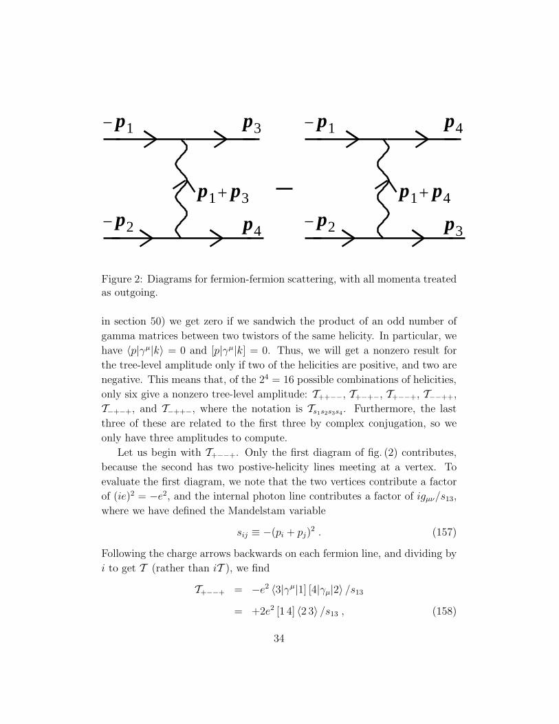


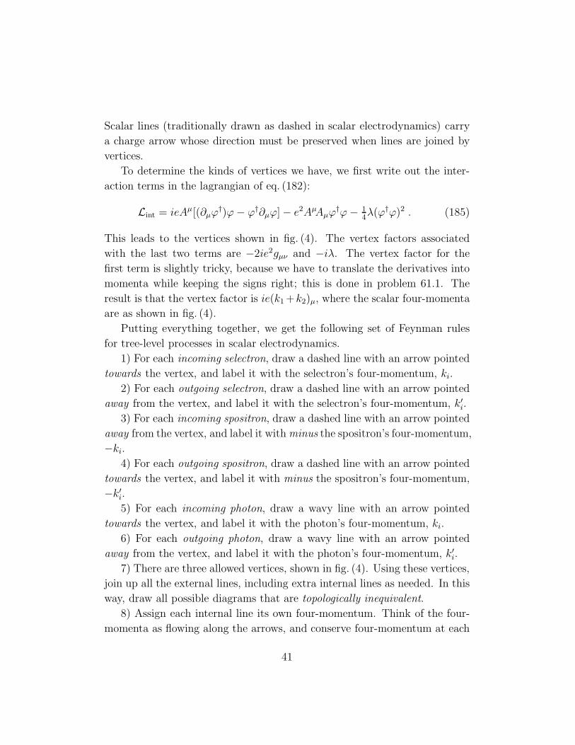
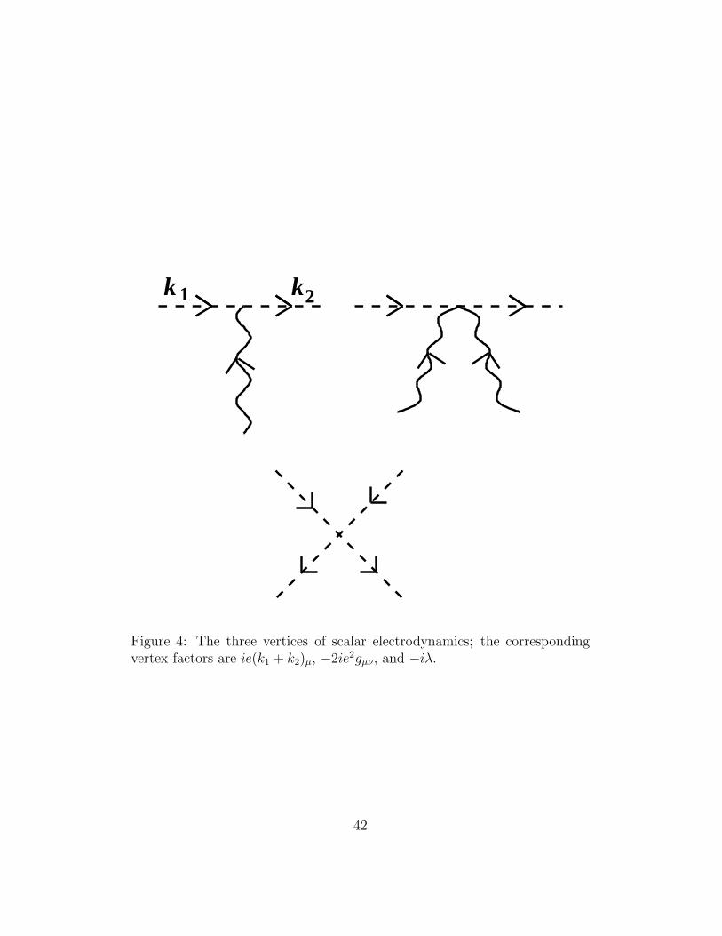

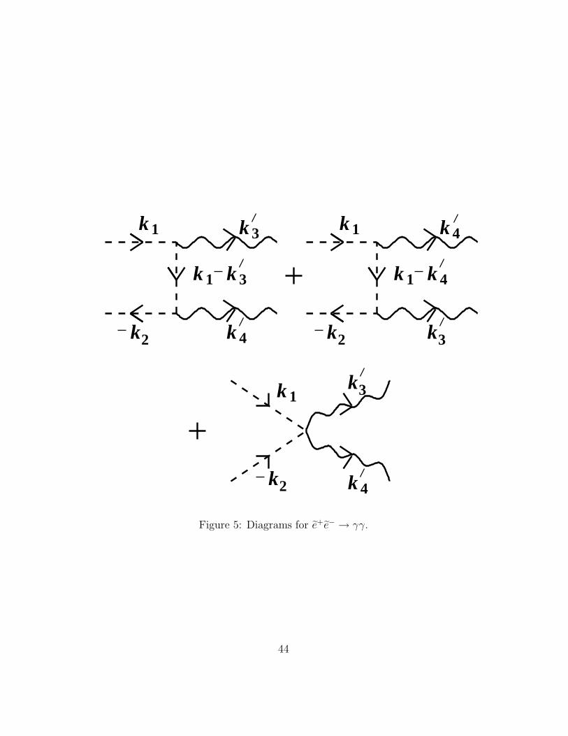


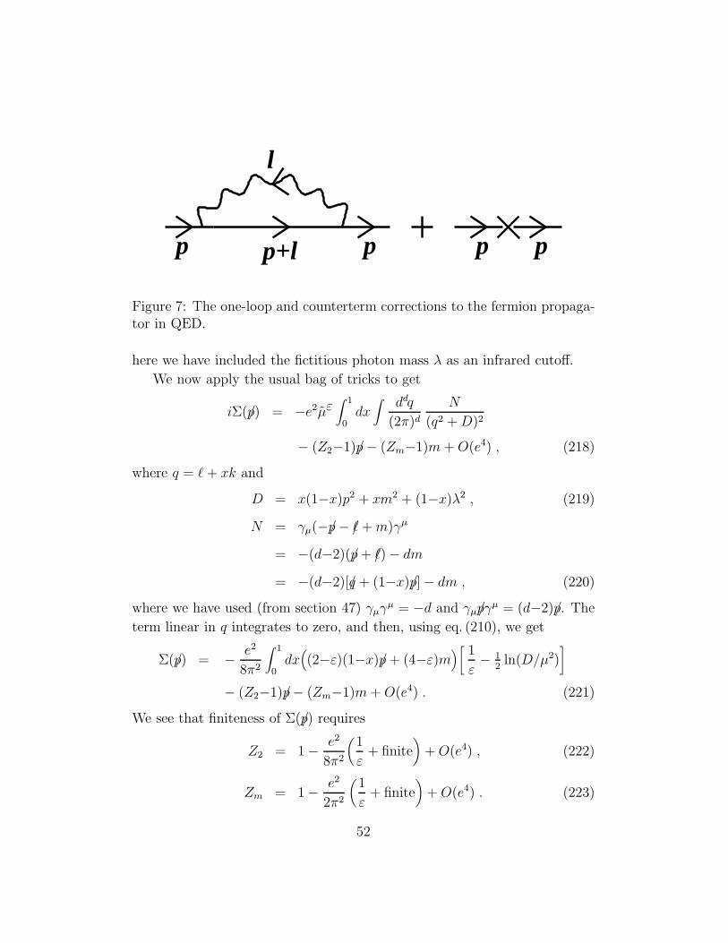


![OBLIQUE CORRECTIONS IN THE DINE-FISCHLER ...diposit.ub.edu/dspace/bitstream/2445/96759/1/TFM_Ast...Dine, Fischler and Srednicki [5] and Zhitnitsky [6] independently proposed a generalization](https://static.documents.pub/doc/80x56/604d2ad984275c165a10e513/oblique-corrections-in-the-dine-fischler-dine-fischler-and-srednicki-5.jpg)


