Notes on Reduced Factorizations of the Symmetric Group

Notes on Reduced Factorizations of the Symmetric Group

David P. Little

February 20, 2004

Abstract

The primary goal of these notes is to provide an introduction to Schubert polynomials

via the theory of reduced factorizations of the symmetric group. To this end, we will

make use of two graphical representations of these reduced factorizations: line and labeled

circle diagrams. To gain an intuitive understanding of the fundamental properties these

factorizations, it is necessary to consider many examples. For this reason, we have developed

the Java application Diagram Viewer. These notes are to also serve as a manual for this

software.

Contents

1 Reduced Words of the Symmetric Group 21.1 Simple Transpositions . . . . . . . . . . . . . . . . . . . . . . . . . . . . . . . . . 21.2 Line Diagrams . . . . . . . . . . . . . . . . . . . . . . . . . . . . . . . . . . . . . 31.3 Labeled Circle Diagrams . . . . . . . . . . . . . . . . . . . . . . . . . . . . . . . . 61.4 The Shape of a Permutation . . . . . . . . . . . . . . . . . . . . . . . . . . . . . . 8

2 Schubert Polynomials 122.1 Difference Operator . . . . . . . . . . . . . . . . . . . . . . . . . . . . . . . . . . 122.2 Weak Bruhat Order and Schubert Polynomials . . . . . . . . . . . . . . . . . . . 152.3 Combinatorial Constructions of Schubert Polynomials . . . . . . . . . . . . . . . 21

3 On the Number of Reduced Factorizations 233.1 Stanley Symmetric Functions . . . . . . . . . . . . . . . . . . . . . . . . . . . . . 233.2 Kadell’s Zig-Zag Rule . . . . . . . . . . . . . . . . . . . . . . . . . . . . . . . . . 243.3 Combinatorial Definition of the Schur Functions . . . . . . . . . . . . . . . . . . 26

4 Multiplication of Schubert Polynomials 294.1 Monk’s Formula . . . . . . . . . . . . . . . . . . . . . . . . . . . . . . . . . . . . 294.2 Multiplication by an elementary symmetric function . . . . . . . . . . . . . . . . 294.3 Conjectured Formulas . . . . . . . . . . . . . . . . . . . . . . . . . . . . . . . . . 29

5 Other Properties of Schubert Polynomials 29

6 Open Problems 29

A Using the Diagram Viewer 30A.1 Introduction . . . . . . . . . . . . . . . . . . . . . . . . . . . . . . . . . . . . . . . 30A.2 Target Mode . . . . . . . . . . . . . . . . . . . . . . . . . . . . . . . . . . . . . . 32A.3 Coxeter Mode . . . . . . . . . . . . . . . . . . . . . . . . . . . . . . . . . . . . . . 32A.4 LS Tree Mode . . . . . . . . . . . . . . . . . . . . . . . . . . . . . . . . . . . . . . 32A.5 General Modes . . . . . . . . . . . . . . . . . . . . . . . . . . . . . . . . . . . . . 32

1

February 20, 2004 Reduced Words and Schubert Polynomials 2

1 Reduced Words of the Symmetric Group

1.1 Simple Transpositions

Our main goal for this section is to understand how a given permutation1 σ = (σ1, σ2, . . . , σn) ∈Sn, can be written as the product of simple transpositions si = (i, i + 1) for 1 ≤ i ≤ n − 1. Forexample, the permutation σ = (3, 5, 1, 4, 2) can be factored as

σ = (4, 5)(2, 3)(3, 4)(1, 2)(4, 5)(2, 3) = s4s2s3s1s4s2.

It will be convenient to think of these factorizations as being built up from left to right,meaning that we are always multiplying by a simple transposition on the right. Notice thatthe action of multiplying σ on the right by si is to simply switch the numbers σi and σi+1, orsymbolically

σsi = (σ1, . . . , σi−1, σi+1, σi, σi+2, . . . , σn).

Multiplying on the left by si has the effect of switching the numbers i and i + 1, which may ormay not be next to each other in σ.

To simplify notation, we will only refer to the indices of the simple transpositions. In otherwords, the above factorization will be indicated by the sequence of numbers 423142.

Definition 1.1 A word w = w1w2 · · ·wk in the alphabet {1, 2, . . . , n − 1} corresponds to σ if

σ = sw1sw2

· · · swk

where k is the length of w.

It is clear that any permutation can be written as the product of simple transpositions byconsidering the product sβ−1sβ−2 · · · sα for α < β. Notice that multiplying σ on the right bythis product yields

σsβ−1sβ−2 · · · sα = (σ1, σ2, . . . , σα−1, σβ , σα, σα+1, . . . , σβ−1, σβ+1, . . . , σn).

In other words, the number σβ has been removed from the permutation and reinserted intoposition α, shifting by one position all numbers to its right. With this in mind, we can constructa factorization of σ by first inserting σ1 into position 1, then inserting σ2 into position 2 and soon. The resulting product will be of the form

σ =

n−1∏

i=1

saisai−1 · · · si+1si (1.1)

where i − 1 ≤ ai ≤ n − 1. If ai = i − 1 then the product sai· · · si is assumed to be empty.

Definition 1.2 The product given in (1.1) is called the canonical factorization of σ.

The canonical factorization of (3, 5, 1, 4, 2) is the word 214324.Since it is now clear that the set {si}

n−1i=1 generates Sn, we shift our focus back to the problem

of finding all factorizations of a permutation into simple transpositions. To this end, we point

1Unless otherwise stated, all permutations (except transpositions) will be written using one-line notation.Transpositions will be written using cycle notation.


out that the simple transpositions satisfy the Coxeter relations

a) s2i = id for 1 ≤ i ≤ n − 1

b) sisj = sjsi for |i − j| ≥ 2

c) sisi+1si = si+1sisi+1 for 1 ≤ i ≤ n − 2.

(1.2)

1.2 Line Diagrams

It will be convenient to think of each factorization in a graphical sense. We will consider twosuch methods, the first being the line diagram.

Definition 1.3 The line diagram of w, denoted LD(w), is the graph of the trajectories of thenumbers 1 through n as they are rearranged into the target permutation σ by the simple transpo-sitions given by w.

Example 1.1 σ = (5, 3, 6, 4, 2, 1), w = 432132543545.

1

1

2

2

3

3

4 4

5

5

6

6

Example 1.2 σ = (5, 3, 6, 4, 2, 1), w = 234312543145.

1

1

2

2

3

3

4 4

5

5

6

6

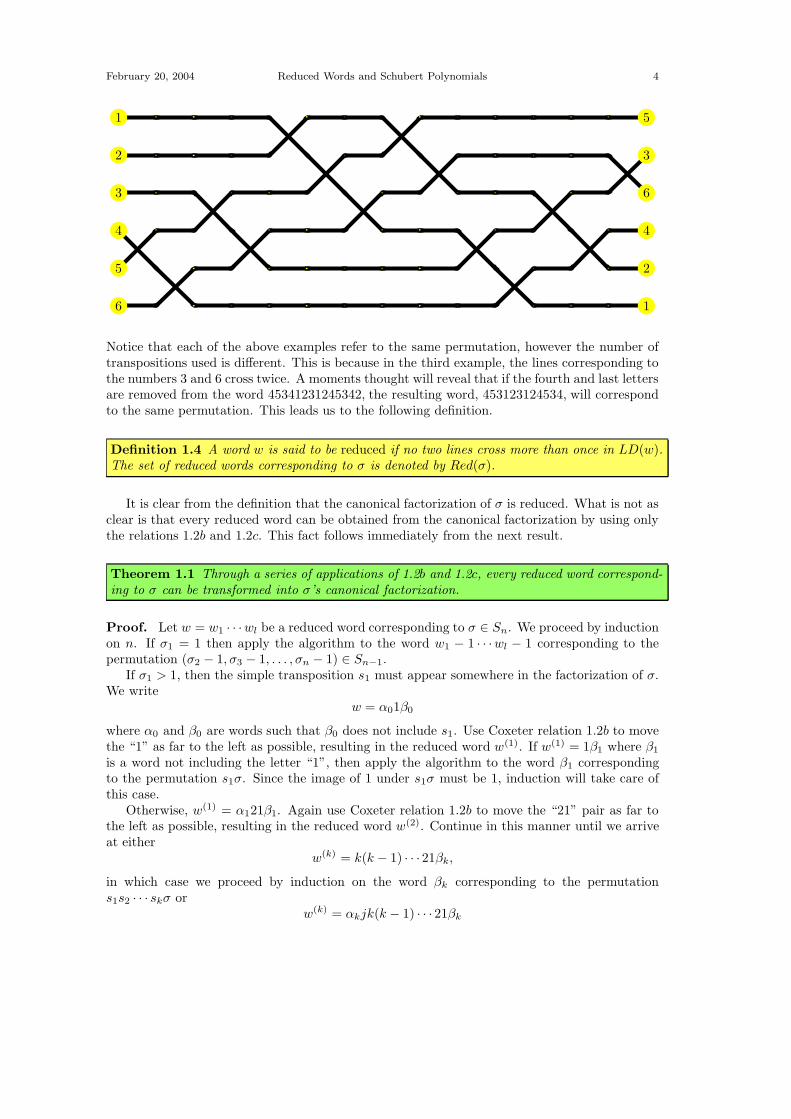
Example 1.3 σ = (5, 3, 6, 4, 2, 1), w = 45341231245342.


1

1

2

2

3

3

4 4

5

5

6

6

Notice that each of the above examples refer to the same permutation, however the number oftranspositions used is different. This is because in the third example, the lines corresponding tothe numbers 3 and 6 cross twice. A moments thought will reveal that if the fourth and last lettersare removed from the word 45341231245342, the resulting word, 453123124534, will correspondto the same permutation. This leads us to the following definition.

Definition 1.4 A word w is said to be reduced if no two lines cross more than once in LD(w).The set of reduced words corresponding to σ is denoted by Red(σ).

It is clear from the definition that the canonical factorization of σ is reduced. What is not asclear is that every reduced word can be obtained from the canonical factorization by using onlythe relations 1.2b and 1.2c. This fact follows immediately from the next result.

Theorem 1.1 Through a series of applications of 1.2b and 1.2c, every reduced word correspond-ing to σ can be transformed into σ’s canonical factorization.

Proof. Let w = w1 · · ·wl be a reduced word corresponding to σ ∈ Sn. We proceed by inductionon n. If σ1 = 1 then apply the algorithm to the word w1 − 1 · · ·wl − 1 corresponding to thepermutation (σ2 − 1, σ3 − 1, . . . , σn − 1) ∈ Sn−1.

If σ1 > 1, then the simple transposition s1 must appear somewhere in the factorization of σ.We write

w = α01β0

where α0 and β0 are words such that β0 does not include s1. Use Coxeter relation 1.2b to movethe “1” as far to the left as possible, resulting in the reduced word w(1). If w(1) = 1β1 where β1

is a word not including the letter “1”, then apply the algorithm to the word β1 correspondingto the permutation s1σ. Since the image of 1 under s1σ must be 1, induction will take care ofthis case.

Otherwise, w(1) = α121β1. Again use Coxeter relation 1.2b to move the “21” pair as far tothe left as possible, resulting in the reduced word w(2). Continue in this manner until we arriveat either

w(k) = k(k − 1) · · · 21βk,

in which case we proceed by induction on the word βk corresponding to the permutations1s2 · · · skσ or

w(k) = αkjk(k − 1) · · · 21βk


with j < k. In this case, use Coxeter relation 1.2b to arrive at

αkk(k − 1) · · · (j + 2)j(j + 1)j(j − 1) · · · 21βk

at which point we now use Coxeter relation 1.2c

αkk(k − 1) · · · (j + 2)(j + 1)j(j + 1)(j − 1) · · · 21βk

followed by a series of applications of Coxeter relation 1.2b

w(k′) = αkk(k − 1) · · · 21(j + 1)βk.

Notice that the letters k(k − 1) · · · 21 have all been shifted one place to the left. It should beclear that we can continue this process until we arrive at the word

w(l) = l(l − 1) · · · 21βl

for some l ≥ k, at which point we can apply the algorithm to the word βl and the proof iscomplete by induction. 2

Remark 1.1 Coxeter relation 1.2a is used only in the transition from a non-reduced word to areduced word. If w is non-reduced, then by definition there are two lines, call them x and y, inLD(w) that cross at least twice. Assume that w is of the form

w = w1 · · ·wi−1αwi+1 · · ·wj−1βwj+1 · · ·wk

where α is the first letter to interchange x and y and β is the second. Without loss of generality,we may also assume that the word w′ = wi+1 · · ·wj−1 is reduced. Notice that lines α and α + 1are adjacent at the beginning and end of LD(w′). This implies that αw′ and w′β are reducedwords corresponding to the same permutation. Using Theorem 1.1, we see that w′β can betransformed into αw′ using only 1.2b and 1.2c. Having done so, the pair αα would appear in ourword and thus we could apply relation 1.2a to decrease the length of the word by two.

Since relations 1.2b and 1.2c do not change the length of a word, all elements of Red(σ) musthave the same length. This allows us to define the length of a permutation.

Definition 1.5 The length of σ, denoted l(σ), is the length of any reduced word correspondingto σ.

Note that it is unnecessary to construct a reduced word in order to determine the length ofa permutation.

Theorem 1.2 The length of σ is given by the number of inversions of σ. Symbolically,

l(σ) =∣

∣{(σi, σj) | i < j and σi > σj}∣

∣.

Proof. It is easy to see from the construction of the canonical factorization that each simpletransposition introduces exactly one new inversion while at the same time preserving the existinginversions. Since the number of inversions of the identity permutation is 0, which is also thelength of the identity, our proof is complete. 2


It will be of later interest to understand the effect on the length function of right multiplicationby the transposition tij = (i, j) where i < j. Certainly if σi < σj , then we have introduced anew inversion, but we could have conceivably introduced or destroyed other inversions as well.Similarly if σi > σj .

Lemma 1.3 Let σ ∈ Sn and 1 ≤ i < j ≤ n. Then

l(σtij) =

{

l(σ) + 1 + 2 |{i < k < j | σi < σk < σj}| if σi < σj

l(σ) − 1 − 2 |{i < k < j | σi > σk > σj}| if σi > σj

1.3 Labeled Circle Diagrams

Our second graphical representation of a word is the labeled circle diagram. We begin byconstructing the circle diagram, a square matrix used to record both the permutation and thecorresponding set of inversions. For a given permutation σ ∈ Sn, construct the circle diagram ofσ, denoted CD(σ), in the following steps

1. Label the rows of an n × n matrix with the numbers 1 through n from top to bottom.

2. Label the columns with the numbers σ1, σ2, . . . , σn from left to right.

3. For each 1 ≤ i ≤ n, place an “×” in the cell in row i and column labelled i.

4. Place a “•” in each cell which is either due east or due south of an “×”.

5. Place a “©” in each cell that is not labeled by an “×” or a “•”.

Example 1.4 σ = (5, 3, 6, 4, 2, 1).

1

2

3

4

5

6

5

× • • • • •

•

3

× • • • •

•

•

•

6

× • • •

4

× • •

•

•

2

× •

•

•

•

•

1

×•

•

•

•

•

mmmmmmmmmmm m

It is not a coincidence that there are exactly 12 “©”s in the circle diagram of a permutationof length 12 as in Example 1.4. This is because each “©” corresponds to a specific inversion,and vice versa. Consider a “©” in row i and column labeled j in a given circle diagram. Thecolumn label j must be bigger than i since the “×” in that column is below the “©”. Likewise,i must appear to the right of j in the permutation because the “×” in row i is to the right ofthe “ ©”. This means that the pair (j, i) is an inversion.

To construct the labeled circle diagram corresponding to w ∈ Red(σ), denoted LCD(w),proceed with the following additional step.

6. For 1 ≤ i ≤ l(σ), if the ith letter of w crosses lines r and s > r in LD(w), label the “©”in row r and the column labeled s with an i.

Example 1.5 σ = (5, 3, 6, 4, 2, 1), w = 432132543545.


1

2

3

4

5

6

5

× • • • • •

•

3

× • • • •

•

•

•

6

× • • •

4

× • •

•

•

2

× •

•

•

•

•

1

×•

•

•

•

•

m4 m6 m9 m11 m12m3 m5 m8 m10m2m1 m7

Example 1.6 σ = (5, 3, 6, 4, 2, 1), w = 234312543145.

1

2

3

4

5

6

5

× • • • • •

•

3

× • • • •

•

•

•

6

× • • •

4

× • •

•

•

2

× •

•

•

•

•

1

×•

•

•

•

•

m6 m5 m9 m11 m12m3 m1 m7 m2m10m4 m8

Note that we have only defined the labeled circle diagram for a reduced word. While thedefinition can be easily extended for any word, the diagram itself can get unnecessarily (for thetime being) complicated.

Remark 1.2 To construct the labeled circle diagram for the canonical factorization, the la-bels 1, 2, . . . , n are placed successively up the columns starting with the left most column andproceeding to the right. This observation leads us to the following definitions.

Definition 1.6 If the cell in row i and column j contains a “©”, then let Hi,j refer to the setof “©”s that are either due east or due south of cell (i, j)2, including cell (i, j). The set Hi,j isreferred to as a hook.

Let w represent the canonical factoization of σ. In light of Remark 1.2, all of the labels inany hook, Hi,j , of LCD(w) must increase as we read up column j and to the right in row i. Ifw does not represent the canonical factorization, then this is certainly not the case, but noticewhat does happen. Consider the hook H2,1 in Example 1.6. The labels appear in the order(4, 10, 3, 1, 7, 2). If these numbers are rearranged into increasing order, the “3” remains in thesame position. This leads us to the following definition.

Definition 1.7 The hook Hi,j is said to be balanced if the number of cells to the right of cell(i, j) that are labeled with a smaller number than cell (i, j) is equal to the number of cells belowcell (i, j) that are labeled with a larger number than cell (i, j).

In other words, upon rearranging the labels of Hi,j into increasing order (bottom to top, leftto right), the label in cell (i, j) remains in the same position. It is not a coincidence that all ofthe hooks in Example 1.6 are balanced.


Theorem 1.4 A labeling of the “©”s in CD(σ) with the numbers 1 through l(σ) correspondsto a reduced word if and only if each hook of CD(σ) is balanced.

Proof. To show that every LCD(w) of a reduced word is balanced, it is enough to show thatCoxeter relations 1.2b and 1.2c preserve this property. To show that every balanced labelingcorresponds to a reduced word, show that there exists an algorithm using Coxeter-like relationsthat converts any balanced labeling to that of the balanced labeling of the canonical factorization.This is left as an exercise to the reader. 2

1.4 The Shape of a Permutation

We now have a completely combinatorial description of a reduced word that should allow us toenumerate such words. In fact, as we will later show for certain permutations, these balancedlabelings are in one-to-one correspondence with another classical combinatorial structure, thestandard Young tableau. To this end, we conclude this section by categorizing certain types ofpermutations.

Definition 1.8 The code of σ, denoted c(σ) is the vector (c1(σ), c2(σ), . . . , cn(σ)) where

ci(σ) = {j > i | σj < σi}

The shape of σ, denoted λ(σ), is the partition corresponding to the decreasing rearrangement ofc(σ).

Remark 1.3 A permutation is uniquely identified by its code. Additionally, a vector(c1, c2, . . . , cn) is the code of a permutation if and only if 0 ≤ ci ≤ n − i for each 1 ≤ i ≤ n.

Another way to think of the code of σ is that it is the vector whose ith component is thenumber of “©”s in the ith column of CD(σ). With this in mind, consider the following defini-tions. We start with the case where there is no difference between the code of σ and the shapeof σ.

Definition 1.9 A permutation is said to be dominant if c(σ) is in decreasing order.

Example 1.7 σ = (7, 8, 5, 6, 4, 3, 1, 2), c(σ) = (6, 6, 4, 4, 3, 2, 0, 0)

1

2

3

4

5

6

7

8

7

× • • • • • • •

•

8

× • • • • • •

5

× • • • • •

•

•

•

6

× • • • •

•

•

4

× • • •

•

•

•

•

3

× • •

•

•

•

•

•

1

× •

•

•

•

•

•

•

•

2

×•

•

•

•

•

•

mmmmmmmmmmmmmmmmmmmmmmmmm


If c(σ) is in decreasing order, then the circles in each row of CD(σ) must be left justifiedand the number of circles in each row must be weakly decreasing. That is to say the circles ofCD(σ) form a Ferrers diagram drawn in English notation. To see this, an example should dothe trick. Let’s asumme that we are constructing a dominant permutation σ and so far we haveσ = (7, 4, 5, σ4, . . . , σ8). The partially constructed circle diagram for σ is shown in Figure 1.1.

1

2

3

4

5

6

7

8

7

× • • • • • • •

•

4

× • • • • • •

•

•

•

•

5

× • • • • •

•

•

•

mmmmmmmmmmmm

Figure 1.1:

What are the possible values for σ4 so that c4(σ) ≤ c3(σ)? If σ4 ∈ {1, 2, 3} then c4(σ) < c3(σ).If σ4 = 6 then c4(σ) = c3(σ). Otherwise, c4(σ) > c3(σ). In general, if we have selected σ1 throughσi such that c1(σ) ≥ · · · ≥ ci(σ) then the “×” in the (i + 1)st column must be placed in oneof the first ci(σ) + 1 available rows to insure that ci(σ) ≥ ci+1(σ). If so, then the circles in the(i + 1)st would appear precisely in rows 1 through ci(σ).

Remark 1.4 The circle diagram of a dominant permutation can be broken up into two regionsdepending on whether or not a cell contains a “©”. The boundary between these two regionscan be thought of as a lattice path from the lower left hand corner to the upper right cornerof CD(σ). In light of Remark 1.3 (i.e. ci(σ) ≤ n − i), this path must stay weakly above thediagonal from the lower left to the upper right. Conversely, any such path must give rise toa dominant permutation. This says that the number of dominant permutations of Sn is thenumber of lattice paths from (0, 0) to (n, n) that stay weakly above the line y = x, which is thenth Catalan number,

(

2nn

)

/(n + 1).

Another defining property of a Ferrers diagram is that if cell (i, j) is in the diagram, thenthe set of cells {(a, b) | a ≤ i & b ≤ j} must also be in the diagram. In other words, all cellsto the northwest of cell (i, j) must be in the diagram if cell (i, j) is in the diagram. What doesthis say about σ if the circles of CD(σ) form a Ferrers diagram? Assume that there is a “©”in cell (σk , j). Then the “×” in the jth column must appear below row σk and the “×” in rowσk must appear to the right of the jth column, as illustrated in Figure 3.8.


σk

σj

σj σk

m

×

×

Figure 1.2:

If there was an “×” northwest of cell (σk, j), say in cell (σi, i), then there exists three indicesi < j < k such that σi < σk < σj . We say that the numbers (σi, σj , σk) form a “132” pattern.But since this can not happen when σ is dominant, we say that σ avoids the pattern 132, or is132-avoiding. In other words, σ is dominant if and only if it is 132-avoiding.

This notion of a “pattern” can be extended to any permutation α = (α1, . . . , αk) ∈ Sk. Fora given permutation σ ∈ Sn and indices 1 ≤ i1 < i2 < · · · < ik ≤ n, (σi1 , σi2 , . . . , σik

) is an αpattern if for each j, σij

is the αthj smallest number. If σ contains no such pattern, then we say

that σ avoids α or is α-avoiding.

Definition 1.10 A permutation is said to be 321-avoiding if there does not exist indices i < j <k such that σk < σj < σi

Example 1.8 σ = (3, 1, 7, 2, 8, 4, 5, 6) is 321-avoiding.

1

2

3

4

5

6

7

8

3

× • • • • • • •

•

•

•

•

•

1

× • • • • • •

•

•

•

•

•

•

•

7

× • • • • •

•

2

× • • • •

•

•

•

•

•

•

8

× • • •

4

× • •

•

•

•

•

5

× •

•

•

•

6

×•

•

mm m

m mm mm m

In terms of the circle diagram, a 321-avoiding permutation can be indentified in the followingmanner. First remove all rows and columns that do not contain any circles. If in what remainsthe circles form a Ferrers diagram of French skew shape, then the permutation is 321-avoiding.We leave this as an exercise to the reader.

Another interesting fact is that every word w ∈ Red(σ) contains the same multiset of lettersif σ is 321-avoiding. In other words, each reduced word corresponding to σ can be transformedinto the canonical factorization of σ using only Coxeter relation 1.2b. The basic reason for thisis that 121 and 212 are the only reduced words for the permutation 321, which are of courserelated by Coxeter relation 1.2c.

Definition 1.11 A permutation is said to be vexillary if it is 2143-avoiding.


Example 1.9 σ = (4, 8, 7, 2, 5, 3, 6, 1) is vexillary.

1

2

3

4

5

6

7

8

4

× • • • • • • •

•

•

•

•

8

× • • • • • •

7

× • • • • •

•

2

× • • • •

•

•

•

•

•

•

5

× • • •

•

•

•

3

× • •

•

•

•

•

•

6

× •

•

•

1

×•

•

•

•

•

•

•

mmmmmmmmmmmmm m

mmmmm

Notice that in the above example, the columns of circles can be totally ordered by set inclu-sion. In other words, if we define Cj(σ) = {i | cell (i,j) of CD(σ) is a ©}, then the Cj ’s can beordered by set inclusion. The same thing can be said about the rows. It turns out that theseproperties of CD(σ) hold if and only if σ is vexillary.

Another equivalent definition of vexillary is that λ(σ)′ = λ(σ−1), where λ(σ)′ denotes theconjugate shape of λ(σ) (i.e. λ(σ)′ is the vector whose ith component is the number of compo-nents of λ(σ) whose value is at least i) Again, we leave the proof of this fact as an exercise.

Remark 1.5 Dominant permutations are necessarily vexillary.

Definition 1.12 A permutation is said to be Grassmanian if it has only one descent.

Example 1.10 σ = (2, 4, 7, 8, 1, 3, 5, 6) is Grassmanian.

1

2

3

4

5

6

7

8

2

× • • • • • • •

•

•

•

•

•

•

4

× • • • • • •

•

•

•

•

7

× • • • • •

•

8

× • • • •

1

× • • •

•

•

•

•

•

•

•

3

× • •

•

•

•

•

•

5

× •

•

•

•

6

×•

•

mmmm

mmm

mmmm

In the case of Grassmanian permutations, it’s clear that once the rows and columns whichare void of circles are removed from CD(σ), the remaining cells which contain circles form aFerrers diagram where the rows are right justified.

Remark 1.6 Grassmanian permutations are both 321-avoiding and vexillary.


2 Schubert Polynomials

2.1 Difference Operator

Let f be a polynomial in n variables. Define the difference operator ∂i by

∂if(x1, . . . , xn) =f(. . . , xi, xi+1, . . .) − f(. . . , xi+1, xi, . . .)

xi − xi+1.

It will be convenient to use the shorthand notation given by

∂i =1

xi − xi+1(1 − si)

where si acts on polynomials by switching variables xi and xi+1.

Remark 2.1 It follows directly from the definition that for any polynomial f , ∂if is symmetricin the variables xi and xi+1. Additionally, if f is symmetric in xi and xi+1 then ∂if = 0.

Lemma 2.1 For all polynomials f and g, ∂i(fg) = (∂if)g + (sif)∂ig

Proof.

∂i(fg) =fg − si(fg)

xi − xi+1

=fg − (sif)g + (sif)g − si(f)si(g)

xi − xi+1

=f − sif

xi − xi+1g + (sif)

g − sig

xi − xi+1= (∂if)g + (sif)∂ig

2

Corollary 2.2 If f is symmetric in xi and xi+1 then for any polynomial g, ∂i(fg) = f∂ig

Proof. This is an immediate consequence of Remark 2.1 and Lemma 2.1. 2

Theorem 2.3 The operator ∂i satisfies the following properties

a) ∂2i = 0 for 1 ≤ i ≤ n − 1

b) ∂i∂j = ∂j∂i for |i − j| ≥ 2

c) ∂i∂i+1∂i = ∂i+1∂i∂i+1 for 1 ≤ i ≤ n − 2

(2.1)

Proof. Equation 2.1a is an immediate consequence of Remark 2.1. Equation 2.1b follows fromthe fact that ∂i and ∂j act on a completely different set of variables. Equation 2.1c is somewhatmore cumbersome to prove. We first calculate ∂i+1∂i by applying Lemma 2.1.


∂i+1∂i = ∂i+11

xi − xi+1(1 − si)

= ∂i+1

(

1

xi − xi+1

)

(1 − si) + si+11

xi − xi+1∂i+1(1 − si)

=1

xi+1 − xi+2

(

1

xi − xi+1−

1

xi − xi+2

)

(1 − si) +1

xi − xi+2∂i+1(1 − si)

=1

(xi − xi+1)(xi − xi+2)(1 − si) +

1

(xi − xi+2)(xi+1 − xi+2)(1 − si+1)(1 − si)

= A + B

Since ∂i is a linear operator, we can compute ∂i∂i+1∂i as ∂iA + ∂iB.

∂iA = ∂i

(

1

(xi − xi+1)(xi − xi+2)

)

(1 − si) + si1

(xi − xi+2)(xi − xi+1)∂i(1 − si)

=1

xi − xi+1

(

1

(xi − xi+2)(xi − xi+1)−

1

(xi+1 − xi+2)(xi+1 − xi)

)

(1 − si)

+1

(xi+1 − xi+2)(xi+1 − xi)

1

xi − xi+1(1 − si)

2

=1

(xi − xi+1)2

(

1

xi − xi+2+

1

xi+1 − xi+2

)

(1 − si) −2

(xi+1 − xi+2)(xi − xi+1)2(1 − si)

=1

(xi − xi+1)2

(

1

xi − xi+2−

1

xi+1 − xi+2

)

(1 − si)

= −1

(xi − xi+1)(xi − xi+2)(xi+1 − xi+2)(1 − si)

Calculating ∂iB is much easier due to the fact that Corollary 2.2 applies.

∂iB =1

(xi − xi+2)(xi+1 − xi+2)∂i(1 − si+1)(1 − si)

=1

(xi − xi+2)(xi+1 − xi+2)(xi − xi+1)(1 − si)(1 − si+1)(1 − si)

Combining the two previous calculations yields

∂i∂i+1∂i =1

(xi − xi+1)(xi − xi+2)(xi+1 − xi+2)(−1 + (1 − si)(1 − si+1)) (1 − si)

=1

(xi − xi+1)(xi − xi+2)(xi+1 − xi+2)(1 − si − si+1 + sisi+1 + si+1si − sisi+1si)

=1

(xi − xi+1)(xi − xi+2)(xi+1 − xi+2)

∑

σ∈S{i,i+1,i+2}

sign(σ)σ.

Calculating ∂i+1∂i∂i+1 in a similar manner leads to exactly the same conclusion. 2

These properties satisfied by the difference operator ∂i are referred to as the Nil Coxeterrelations due to their similarities to the Coxeter relations. In fact, the arguments used in theproof of Theorem 1.1 and in Remark 1.1 could just as well be applied to ∂i. In other words, ifwe use the convention that for any word w = w1w2 · · ·wk, ∂w is the operator defined by

∂w = ∂w1∂w2

· · · ∂wk


then 2.1a and Remark 1.1 imply that ∂w = 0 unless w ∈ Red(σ) for some σ. Furthermore,relations 2.1b and 2.1c and the technique used in the proof of Theorem 1.1 imply that ∂w = ∂v

for all w, v ∈ Red(σ). Therefore we can unambiguously define ∂σ for σ ∈ Sn as

∂σ = ∂w

for any w ∈ Red(σ).It is appropriate to point out here that for the permutation of maximal length, ω0 =

(n, n − 1, . . . , 2, 1), ∂ω0can be used to generate the Schur functions, Sλ. This can be seen

as a consequence of the following result.

Lemma 2.4

∂ω0=

1∏

1≤i<j≤n

(xi − xj)

∑

σ∈Sn

sign(σ)σ.

Proof. Using the canonical factorization of ω0, we have that

∂ω0=

n−1∏

i=1

∂n−1∂n−2 · · · ∂i

=

n−1∏

i=1

1

xn−1 − xn(1 − sn−1)

1

xn−2 − xn−1(1 − sn−2) · · ·

1

xi − xi+1(1 − si). (2.2)

Therefore we can expand ∂ω0as a sum of permutations in Sn with coefficients in Z(x1, . . . , xn),

or symbolically

∂ω0=

∑

σ∈Sn

cσ(X)σ.

Notice that for any j, the word j∏n−1

i=1 (n−1)(n−2) · · · i is not reduced since ω0 was of maximallength. Therefore ∂j∂ω0

= 0. Or equivalently, ∂ω0is symmetric in xj and xj+1, i.e.

∂ω0= sj∂ω0

.

But since this is true for any j, we must have that

∂ω0= α∂ω0

and thusαcσ(X) = cασ(X) (2.3)

for any two permutations α, σ ∈ Sn. Therefore we need only compute one value of cσ(X). Inparticular, we have

cω0(X)ω0 =

n−1∏

i=1

1

xn−1 − xn(−sn−1)

1

xn−2 − xn−1(−sn−2) · · ·

1

xi − xi+1(−si)

=n−1∏

i=1

1

xn−1 − xn

1

xn−2 − xn· · ·

1

xi − xn(−1)n−isn−1sn−2 · · · si

=∏

1≤i<j≤n

1

(xi − xj)sign(ω0)ω0

Combining this with 2.3 yields

cσ(X) = σω0cω0(X) = σω0

∏

1≤i<j≤n

1

(xi − xj)sign(ω0)

=∏

1≤i<j≤n

1

(xi − xj)sign(σ).


2

Corollary 2.5 For any partition λ = (λ1, λ2, . . . , λn) we have that

∂ω0(xλ1+n−1

1 xλ2+n−22 · · ·xλn

n ) = Sλ(x1, . . . , xn).

Proof. This is an immediate consequence of Lemma 2.4 and the determinantal definition ofthe Schur function

Sλ(x1, . . . , xn) =det |x

λj+n−ji |

det |xn−ji |

.

Notice that det |xn−ji | and

∏

i<j(xi −xj) are monic homogeneous polynomials of degree(

n2

)

,both of which are zero whenever xi = xj for i < j. Therefore they are identical. 2

Definition 2.1 The Schubert polynomial corresponding to ω ∈ Sn is given by

Sω(X) = ∂ω−1ω0(xn−1

1 xn−22 · · ·xn−n

n ) (2.4)

2.2 Weak Bruhat Order and Schubert Polynomials

The Coxeter relations induce a natural partial ordering on Sn.

Definition 2.2 For α, β ∈ Sn we say that α precedes β, denoted α ≺ β, if

i) β = αsi for some i and

ii) l(β) = l(α) + 1.

Weak Bruhat order is defined to be the transitive closure of ≺.

Example 2.1 The order diagrams for weak Bruhat order on S3 and S4 are shown in Figures2.3 and 2.4, respectively. The edge joining the permutations α and β is labeled i if β = αsi.

321

231 312

213 132

1231

2

1

2

1

2

Figure 2.3: Order diagram for weak Bruhat order on S3

In order to compute Schubert polynomials from their definition, it is helpful to think of areduced word for ω as a path from the identity to ω in the order diagram for weak Bruhat order.Similary, we can think of each path from ω to ω0 as a reduced word for ω−1ω0. In other words,


4321

431242313421

41324213

3412

24313241

3214

2341

3142 2413

1432

4123

2314 3124

2143

1342 1423

2134 1324 1243

1234

32

1

2

3

3

1

1

2

23

1

31

21 2

3

3

1

2

1

21

3

2

3

1

22 31

3

12

3

Figure 2.4: Order diagram for weak Bruhat order on S4

to compute Sω using Definition 2.1, apply the operator ∂i upon crossing an edge labeled i whentraversing a path from ω0 to ω. That is to say formally

Sα(X) = ∂iSβ(X) (2.5)

if β = αsi and α precedes β in weak Bruhat order. Repeated applications of (2.5) yields

Lemma 2.6 Let u, v ∈ Sn. Then

∂uSv =

{

Svu−1 if l(v) = l(vu−1) + l(u)

0 otherwise.

For example, using Figure 4.1 in computing S3142, we could first apply ∂1 to x31x

22x3, then


x21x2

x1x2 x21

x1 x1 + x2

1

Figure 2.5:

∂3 and finally ∂2.

S3142 = ∂2∂3∂1(x31x

22x3)

= ∂2∂31

x1 − x2(x3

1x22x3 − x3

2x21x3) = ∂2∂3(x

21x

22x3)

= ∂21

x3 − x4(x2

1x22x3 − x2

1x22x4) = ∂2(x

21x

22)

=1

x2 − x3(x2

1x22 − x2

1x23) = x2

1(x2 + x3)

The complete set of Schubert polynomials for S3 and S4 are given in Figures 2.5 and 2.6,respectively.

We conclude this section by calculating the Schubert polynomials for permutations of a giventype. To this end, we present the following characteristics of Schubert polynomials correspondingto any permutation.

Lemma 2.7 Let ω = (ω1, . . . , ωn) ∈ Sn.

1. Sid(X) = 1

2. Sω(X) is a non-zero homogeneous polynomial of degree l(ω) whose monomials are of theform xα1

1 · · ·xαnn where 0 ≤ αi ≤ n − i

3. Sω(X) is symmetric in xi and xi+1 if and only if ωi < ωi+1

4. If r is the last descent of ω, then Sω(X) ∈ Z[x1, . . . , xr] and Sω(X) 6∈ Z[x1, . . . , xr−1].

Proof.

1. Using Corollary 2.5, we have that Sid(X) = ∂ω0(xn−1

1 · · ·xn−nn ) = S∅(X) = 1.

2. Consider the result of applying ∂i to any monomial of the form xai xb

i+1 where a ≥ b.

∂ixai xb

i+1 =xa

i xbi+1 − xb

ixai+1

xi − xi+1= xb

ixbi+1

xa−bi − xa−b

i+1

xi − xi+1= xb

ixbi+1

a−b∑

j=1

xa−b−ji xj−1

i+1

which is a homogeneous polynomial in xi and xi+1 of degree a + b − 1. Furthermore, theexponent of xi is no more than a − 1 and since ∂ix

ai xb

i+1 is symmetric in xi and xi+1, theexponent of xi+1 is no more than a − 1 as well.

3. Sω(X) being symmetric in xi and xi+1 means that ∂iSω(X) = 0. Lemma 2.6 impliesthat l(ω) = l(ωsi) − 1. In other words, multiplying ω on the right by si introduces a newinversion, which happens if and only if ωi < ωi+1.


x31x

22x3

x31x

22x3

1x2x3x21x

22x3

x31(x2 + x3)x3

1x2

x21x

22

x1x2x3(x1 + x2)x21x2x3

x21x2

x1x2x3

x21(x2 + x3)

x1x2(x1 + x2)

x21x2 + x2

1x3 + x1x22 + x1x2x3 + x2

2x3

x31

x1x2 x21

x21 + x1x2 + x1x3

x1x2 + x1x3 + x2x3 x21 + x1x2 + x2

2

x1 x1 + x2 x1 + x2 + x3

1

Figure 2.6:

4. If r is the last descent of ω, then we must have

ωr > ωr+1 < ωr+2 < · · · < ωn.

Therefore Sω(X) is symmetric in xr+1 through xn, from part 3. Since Sω(X) can notcontain the variable xn, it can not involve any of the variables xr+1 through xn−1 either.However, it must contain the variable xr. If it did not, Sω(X) would be symmetric in xr

and xr+1, which would contradict the fact that ωr > ωr+1.

2

We are now in a position where we can easily calculate Schubert polynomials for certaintypes of permutations.

Lemma 2.8 Ssi(X) = x1 + · · · + xi

Proof. Part 2 of Lemma 2.7 implies that Ssi(X) is homogeneous of degree 1. Part 4 of Lemma

2.7 implies that it is a polynomial in the variables x1 through xi. Part 3 of Lemma 2.7 impliesthat it is symmetric in the variables x1 through xi. Therefore Ssi

(X) = c(x1 + · · ·+xi) for some


c. Applying ∂i to Ssi(X) yields

c = ∂iSsi(X) = Sid(X) = 1

2

Lemma 2.9 If ω is dominant of shape λ then

Sω(X) = xλ1

1 · · ·xλn

n = xλ.

Proof. We will proceed by descent induction on l(ω). It is true for the case ω = ω0, sinceλ(ω) = (n−1, . . . , 2, 1, 0) and Sω(X) = xλ(ω). Now comsider any dominant permutation ω 6= ω0

of shape λ. Find the minimum value r such that λ′r < n − r where λ′ is the conjugate shape of

λ (i.e. λ′i = |{j | λj ≥ i}|). In the case that ω is dominant, λ′

i is simply the number of “©”s inthe ith row of CD(ω).

Let a = λ′r + 1. Note that λa = λa+1 and that ωsa is dominant of length l(ω) + 1 and shape

λ + (0, . . . , 0, 1, 0, . . . , 0), where the 1 appears in the ath position. Therefore

Sω(X) = ∂aSωsa(X) = ∂a(xλ(ωsa)) = ∂a(xaxλ(ω)) = xλ(ω).

2

Lemma 2.10 If ω is Grassmanian with ωr > ωr+1 then

Sω(X) = Sλ(ω)(x1, . . . , xr).

Proof. Since ω is Grassmanian, we must have

c(ω) = (ω1 − 1, ω2 − 2, . . . , ωr − r, 0, . . . , 0)

andλ(ω) = (ωr − r, . . . , ω2 − 2, ω1 − 1).

Let u = (r, r − 1, . . . , 2, 1) ∈ Sr. Notice that ωu = (ωr, . . . , ω2, ω1, ωr+1, . . . , ωn) is dominantwith

λ(ωu) = (ωr − 1, . . . , ω2 − 1, ω1 − 1) = λ(ω) + (r − 1, r − 2, . . . , 1, 0) = λ(ω) + δr

andl(ωu) = l(ω) + l(u).

Applying Lemma 2.6 yields

Sω(X) = ∂uSωu(X) = ∂u(xλ(ωu)) = ∂u(xλ(ω)+δr ) = Sλ(ω)(x1, . . . , xr).

2

We conclude this section with

Theorem 2.11Sω(X) = Sω⊗1(X)


Remark 2.2 this implies that Sω is well-defined for any ω ∈ S∞.

Our next goal will be to construct the Schubert polynomial for any permutation.


2.3 Combinatorial Constructions of Schubert Polynomials

Billey, Jockusch and Stanley (1993) showed that

Theorem 2.12

Sω(X) =∑

a ∈ Red(w)a = a1a2 · · · al

∑

1 ≤ b1 ≤ b2 ≤ · · · ≤ bl

ai < ai+1 ⇒ bi < bi+1

bi ≤ ai

xb1xb2 · · ·xbl. (2.6)

Sequences b = (b1, . . . , bl) satisfying the conditions of the inner summation in (2.6) arereferred to as a-compatible.

Example 2.2 Red(1432) = {232, 323}. For the word a = 232, the only a-compatible sequenceis 122. For a = 323, the set of a-compatible sequences is {112, 113, 123, 223}. Therefore

S1432(X) = x1x22 + x2

1x2 + x21x3 + x1x2x3 + x2

2x3.

introduce diagram and D(w) as being the circles of a circle diagramKohnert’s Construction (1990) To construct the set of all Let D refer to any subset of [n]×[n].

We will refer to D as a diagram. Choose a point (i, j) ∈ D such that

i) (i′, j) 6∈ D for all i′ > i

ii) (i, j′) 6∈ D for some j′ < j

Let D′ denote the set obtained from D by replacing (i, j) with (i, k) where k = max{j ′ <j | (i, j′) 6∈ D}. Let K(D) denote the set of diagrams obtained from D (including D itself) by asequence of such operations. And finally, let

xD =∏

(i,j)∈D

xj .

The Schubert polynomial can be constructed as follows

Theorem 2.13Sω(X) =

∑

D∈K(D(ω))

xD

where D(ω) = {(i, j) | cell (i, j) of CD(ω) contains a ©}.

Example 2.3 σ = 1432

mmm

mmm

mmm

m mm

mmm

ThereforeS1432(X) = x2

2x3 + x1x2x3 + x1x22 + x2

1x3 + x21x2.


Kohnert’s formula was originally proved in the case when ω is vexillary. Nantel Bergeronsubsequently proved that a similar but slightly more difficult construction produced the Schubertpolynomials for any permutation. For a proof of Bergeron’s algorithm and a sketch of theequivalence between Bergeron’s and Kohnert’s see...

Fomin, Greene, Reiner and Shimozono A labeling, T , of a diagram D is simply a functionfrom D to Z

+. A labeling is said to be balanced if each of its hooks are balanced. A balancedlabeling is said to be row-strict if no row contains two equal labels. The weight of T , xT , is givenby

xT =∏

(i,j)∈D

xT (i,j).

Theorem 2.14Sω(X) =

∑

T

xT

where the sum is over balanced row-strict labelings of D(ω) such that T (i, j) ≤ j for all (i, j).

Example 2.4 σ = 1432

m1 m2m1

m1 m3m1

m2 m3m1

m2 m1m2

m2 m3m2

ThereforeS1432(X) = x2

1x2 + x21x3 + x1x2x3 + x1x

22 + x2

2x3.


3 On the Number of Reduced Factorizations

While it is evident that Schubert polynomials are not always symmetric functions, it turns outthat if one removes the condition “bi ≤ ai” in the combintorial defintion of Sω(X) given in 2.6,the result is completely symmetric. The resulting functions are known as Stanley symmetricfunctions or stable Schubert polynomials. Using these functions, we are able to give a completeanswer for the number of reduced factorizations of any permutation.

3.1 Stanley Symmetric Functions

Definition 3.1 Let w = w1 · · ·wl ∈ Red(σ). The descent set of w, denoted Des(w), is given by

Des(w) = {i | wi > wi+1}.

Fσ(X) =∑

a ∈ Red(σ)a = a1a2 · · · al

∑

b1 ≤ b2 ≤ · · · ≤ bl

ai > ai+1 ⇒ bi < bi+1

xb1xb2 · · ·xbl. (3.1)

define Φ(σ) (not necessarily the LS Tree) state theorem

Theorem 3.1Fσ(X) =

∑

σ′∈Φ(σ)

Fσ′(X) (3.2)

A similar argument can be used to prove the more general theoremFor any permutation u ∈ Sn and 1 ≤ r ≤ n, we have

∑

σ∈Ψ(u,r)

Fσ(X) =∑

σ∈Φ(u,r)

Fσ(X) (3.3)

where

Φ(u, r) =

{

{uti,r | i ∈ I(u, r)} if I(u, r) 6= ∅

Φ(1 ⊗ u, r + 1) otherwise

Ψ(u, r) =

{

{utr,s | s ∈ S(u, r)} if S(u, r) 6= ∅

Ψ(u ⊗ 1, r) otherwise

where

1 ⊗ u =

(

1 2 . . . n n + 11 u1 + 1 u2 + 1 . . . un + 1

)

and

u ⊗ 1 =

(

1 2 . . . n n + 1u1 u2 . . . un n + 1

)

.


ma

mb

mb

ma

ma

mc mb

mb

mc ma

Figure 3.7:

3.2 Kadell’s Zig-Zag Rule

For a given word w ∈ Red(σ), the line diagram, LD(w), and the labeled circle diagram, LCD(w),both encode the word in a graph. Since it is easy to detect the descents of w using LD(w), it isnatural to ask how we can identify the descents of w using LCD(w). To this end, Kevin Kadellintroduced the notion of the “Zig-Zag” order.

Definition 3.2 Given two labels, a < b, where label a appears in cell (i, j) and label b appearsin cell (i′, j′) with i 6= i′ and j 6= j′. The Zig-Zag order of the following four cells is given by

(i, j′) < (i, j) < (i′, j′) < (i′, j).

The four cells listed above will be referred to as the corner cells.

The four distinct scenarios of the Zig-Zag order are depicted in Figure 3.7. Empty cells couldcontain an “×”, a “•”, or a labeled “©”. In the last two examples, the upper left cell mustcontain a label.

Theorem 3.2 (Kadell) Let w ∈ Red(σ). Then k is in Des(w) if and only if

1. k and k + 1 are in the same column of LCD(w), or

2. k and k + 1 are not in the same row or column of LCD(w) and

(a) no labels appear in the first and last cells of the Zig-Zag and k is in a row lower thanthat of k + 1, or

(b) the first or last cell of the Zig-Zag contains a label, all of which are in increasing orderas they are encountered in Zig-Zag order.

Proof. Consider the case when k and k + 1 are in the same column of LCD(w). Assume thatk is in cell (i, j) and k + 1 is in cell (i′, j). Then the corresponding section of LD(w) would looklike

σj

σj

i

i

i′

i′

In other words, wk+1 = wk − 1, and thus k would be a descent. What happens if k and k +1are in the same row of LCD(w)? Assume that k is in cell (i, j) and k + 1 is in cell (i, j ′). Thenthe corresponding section of LD(w) would look like


σj′

σj′σj

σji

i

In other words, wk+1 = wk + 1, and thus k would not be a descent of w.Now consider the situation where k and k + 1 are not in the same row or column. Assume

that k appears in cell (i, j) and k + 1 appears in cell (i′, j′).If k is a descent of w, then the corresponding section of LD(w) looks like

σj

σji

i

...

σj′

σj′i′

i′

If i < σj′ then cell (i, j′) of LCD(w) must contain a label less than k since these lines wouldhave to cross prior to the kth letter of w. If i > σj′ then cell (i, j′) must contain a “•”. If i′ < σj

and cell (i′, j) contains a label, then that label must be greater than k+1. If i′ > σj then i < σj′

and cell (i′, j) contains a “•”.Notice that in each of the above cases, the labels appear in increasing order as the cells are

traversed in Zig-Zag order.What if k is not a descent of w? Then the corresponding section of LD(w) looks like

σj′

σj′i′

i′

...

σj

σji

i

If i < σj′ and cell (i, j′) contains a label, then that label must be greater than k + 1. Ifi > σj′ then cell (i, j′) must contain a label less than k. If i′ < σj then cell (i′, j) must containa label less than k. If i′ > σj then i < σj′ and cell (i′, j) contains a “•”.

Notice that in each of the above cases except one, the labels do not appear in increasingorder as the cells are traversed in Zig-Zag order. This one case is when i < σj′ and cell (i, j′)doesn’t contain a label and i′ > σj . The corresponding circle diagram would look like


i

i′

σj σj′

mk

mk + 1

×

.5.5.5

•

•

•

×

.5.5

••

.5.5

•

•

•

•

•

Figure 3.8:

2

Corollary 3.3 If w ∈ Red(σ) and σ is 321-avoiding, then k is a descent of w if and only ifk + 1 appears strictly north and weakly west of k in LCD(w).

Proof. Recall that the circles in the circle diagram for a 321-avoiding permutation form aFrench skew shape λ/µ.

λ/µ

µ

The very nature of this shape and the balanced condition on every labeled circle diagramimplies that the labels must be strictly increasing up each column and left to right along eachrow. Therefore, if k and k + 1 are in the same column, k + 1 must be north of k. If k are k + 1are not in the same row or column and the the first or last cell of the zig-zag contains a label,then k is a descent if and only if k + 1 is strictly northwest of k. 2

3.3 Combinatorial Definition of the Schur Functions

Definition 3.3 A column strict tableau of shape λ, is a filling of the cells of the Ferrers diagramof λ with numbers that weakly increase along the row and strictly increase down each column.The set of all such tableaux is denoted CST (λ). The weight of a tableau T , denoted xT , is givenby

xT =∏

(i,j)∈λ

xT (i,j)

where T (i, j) denotes the entry in cell (i, j) of T .


Theorem 3.4Sλ(x1, . . . , xN ) =

∑

T∈CST (λ)

xT

where T (i, j) ≤ N

The proof of the above theorem goes beyond the scope of the these notes, but assuming thisto be the case, we can easily prove the following fact. The previous definitions can easily beextended to the case of a French skew tableau of shape λ/µ.

Theorem 3.5 If σ is 321-avoiding of French skew shape λ/µ then

Fσ(X) = Sλ/µ(X) (3.4)

Proof. We will demonstrate a bijection between column strict tableaux of shape λ/µ and pairs(w, b) where w = w1 · · ·wl is a reduced word corresponding to a 321-avoiding permutation ofFrench skew shape λ/µ and b is a weakly increasing sequence b1 ≤ · · · ≤ bl such that bi < bi+1

if wi > wi+1.Given T ∈ CST (λ/µ), we will construct LCD(w) and b in the following manner. Assume that

T contains αi i’s. First replace the α1 ones in T with the numbers 1 through α1 as they appearfrom left to right and set b1 = · · · = bα1

= 1. Next replace the α2 twos in T with the numbersα1 + 1 through α1 + α2 as they appear from left to right and set bα1+1 = · · · = bα1+α2

= 2.Given LCD(w) and b, construct T by making the replacement i → bi in LCD(w). The

column strictness of T is guaranteed by Kadell’s Zig-Zag rule. 2

Example 3.1 λ = (5, 5, 3, 1) and µ = (3, 1).

4

2 2 3

1 1 4 5

1 2

8

4 5 7

1 2 9 10

3 6

1,1,1,2,2,2,3,4,4,5

Corollary 3.6 If σ is vexillary of shape λ then

Fσ(X) = Sλ′(X) (3.5)

Remark 3.1 Recall that dominant and Grassmanian permutations are both vexillary.


Remark 3.2 A standard Young tableau of shape λ is a column strict tableau of shape λ whoseentries are the numbers 1 through |λ| = λ1 + · · ·λk. The set of all such tableau is denotedSY T (λ). Therefore the coefficient of x1 · · ·xl in Fσ(X) when σ is dominant is the number ofstandard Young tableau. In other wards,

|SY T (λ(σ))| = |Red(σ)| = |BT (λ)|

where BT (λ) is the set of balanced tableaux of shape λ.Therefore, there ought to be a correspondence between balanced tableaux and standard Youngtableaux. The bijection described in Section 4.1 gives such a correspondence. In 1985, Edel-man and Greene described another bijection using Schutzenberger’s promotion operator and avariation on Robinson-Schensted. It is conjectured that these bijections are identical.

Remark 3.3 We can now give an explicit formula for the number of reduced words for anypermutation σ. The last ingredient is the hook formula

|SY T (λ)| =n!

∏

(i,j)∈λ hi,j

where λ ` n and hi,j(λ) denotes the number of cells in the hook Hi,j .


4 Multiplication of Schubert Polynomials

4.1 Monk’s Formula

For a given permutation u ∈ Sn and 1 ≤ r ≤ n, define the following

I(u, r) = {i < r | l(uti,r) = l(u) + 1}

S(u, r) = {s > r | l(utr,s) = l(u) + 1}

Then we havexrSw =

∑

s∈S(w,r)

Swtrs−

∑

i∈I(w,r)

Swtir(4.1)

andSsr

Sw =∑

i ≤ r < jl(wtij) = l(w) + 1

Swtij. (4.2)

where tij = (i, j).

Example 4.1 ω = 1342 and r = 2. I(ω, r) = {1} and S(ω, r) = {3}.

xrSω(X) = x2(x1x2 + x1x3 + x2x3)

= (x21x2 + x2

1x3 + x1x22 + x1x2x3 + x2

2x3) − (x21x2 + x2

1x3)

= S1432 − S3142

Both equations 4.1 and 4.2 (Monk’s Formula) are consequences of the following

Theorem 4.1 Let f =∑

aixi and ω ∈ S∞. Then

fSω(X) =∑

i < jl(ωtij) = l(ω) + 1

(ai − aj)Sωtij(X).

4.2 Multiplication by an elementary symmetric function

See Symmetric functions, schubert polynomials and degeneracy loci

4.3 Conjectured Formulas

5 Other Properties of Schubert Polynomials

Let Hn be the subgroup of Z[x1, . . . , xn] spanned by {xα1

1 xα2

2 · · ·xαnn | αi ≤ n−i}. The collection

of polynomials {Sw}w∈Snis a Z-basis for Hn.

For all w ∈ Sn, Sw is a polynomial with positive integer coefficients.

6 Open Problems

Find a combinatorial proof of the fact that the coefficients cwuv in the expansion

SuSv =∑

cwuvSw

are positive integers.


A Using the Diagram Viewer

A.1 Introduction

The application Diagram Viewer, available for download at

http://www.math.dartmouth.edu/˜dlittle

can be used to “play” with the machinery we have built up thus far. We invite the reader toexperiment with the diagram viewer to gain an intuitive understanding of the material in thissection. A description of its relevant features follows.

Figure A.9:

File Menu: Under the File menu, you can find the usual commands “New”, “Close” and“Quit”. “New” will open up a new window which is identical to the current active window. Itwill automatically contain the same permutation, same reduced word, same mode, etc. “Close”will close the current active window. If there is only one active window, then the program willshut down. “Quit” will close all active windows and shut down the program.

Edit Menu: The Edit menu offers several commands for altering the current reduced word.The “Undo” and “Repeat” commands go backwards and forwards through the sequence ofreduced words that have brought you to the current word. The “Bump” command applies thebumping algorithm to the current word, assuming that a starting position and direction havebeen specified. The “Change Direction” command toggles between bumping up and bumpingdown. The current direction is indicated by a triangle between the circle and line diagrams. A“N” indicates that the current direction is up while “H” indicates the current direction is down.A “�” indicates that no direction has been specified. Note that you must be in either “LS Tree”


mode or one of the “General Tree” modes for the “Bump” and “Change Direction” commandsto be effective.

The “Invert Word” command replaces the current word by it’s inverse, that is the wordformed by reading the current word from right to left. The “Flip Word” command replaces thecurrent word with it’s complement, that is the word formed by replacing each letter i by n − i.

View Menu: Under the View Menu, you will find three commands which can be used to quicklychange the emphasis of the Diagram Viewer. The “Circle Diagram” command expands the sizeof the circle diagram to it’s maximum size. The “Line Diagram” command expands the size ofthe line diagram to it’s maximum size. “Split Screen” divides the screen into two equal parts,half is used for the circle diagram and the other half for the line diagram. The vertical barbetween the two diagrams can be dragged manually, adjusting the size of the two diagrams asdesired.

The “Show All” command toggles the drawing of all numbers in the line diagram. The “ShowBoundary” command toggles the drawing of the boundary in the line diagram.

Mode Menu: You may select from five different Viewer modes using the ”Mode” menu at thetop of the screen. The current available modes include “Target”, “Coxeter”, “LS Tree”, “GeneralTree (1)” and “General Tree (2)”. The significance of these modes is described in the followingsections.

Choice Bars: There are two choice bars located in the lower left corner of the window. The firstmenu allows one to select the value of n anywhere from 3 to 20. If this is not enought, the usermay input permutations of any size manually (see Text Fields below). The second bar allowsthe user to select the type of permutation. The current choices are “Any”, “321-Avoiding”, “Al-ternating”, “Dominant”, “Grassmanian”, “Staircase”, “Reverse”, and “Vexillary”. The “alter-nating” permutation of size 2n is the permutation (2, 1, 4, 3, 6, 5, . . . , 2n, 2n−1). The ”staircase”permutation of size 2n is (n + 1, 1, n + 2, 2, . . . , 2n, n). The “reverse” permutation of size n is(n, n − 1, n − 2, . . . , 2, 1). All other types of permutations refer to a collection of permutations.Changing the value of n or the type of the permutation will produce a randomly selected reducedword corresponding to a permutation in Sn of the specified type.

Buttons: The two buttons, “Random Permutation” and “Random Reduced Word” are virtuallyself-explanatory. The “Random Permutation” button produces a random permutation of n ofthe specified type as well as a random reduced word corresponding to the permutation. The“Random Reduced Word” button produces a random reduced word corresponding to the currentpermutation. The current permutation and reduced word are displayed in the text fields to theright of each button. The only piece of information regarding these buttons that is not obvious,is the fact that holding down the “Shift” key on the keyboard while at the same time pressingeither button will result in the canonical factorization.

The two buttons, “Undo” and “Apply”, in the lower right corner of the window will beexplained in a later section.

Text Fields: The text fields immediately to the right of the buttons display the current per-mutation and word. Note that the word does not need to be reduced. To manually enter apermutation or word, simply type the permutation or word into the appropriate text field andpress “Return”. Make sure that each pair of numbers is separated by a comma. If the usermanually enters a permutation, pressing “Return” will produce a random reduced word corre-sponding to the new permutation. If the user manually enters a word, pressing “Return” willdetermine the permutation automatically.

Permutation Bar: Towards the bottom of the window, above the buttons and text fields,you should see the permutation written out horizontally in black lettering in yellow circles. In


”Coxeter” and ”LS Tree” mode, these don’t do anything. Their functionality in modes ”GeneralTree (1)” and ”General Tree (2)” will be described in a later section.

You should also see two “+” signs to the left and right of the permutation described above.The left ”+” adds one to each number in the permutation and inserts a “1” in front. The right“+” inserts “n+1” at the end of the permutation.

Permutation Type: The type of the current permutation is highlighted at the top of eachwindow. For example, if a permutation is vexillary, then the word “Vexillary” will be highlightedin red. Additionally, if the current word is reduced, then the word “Reduced” will be highlightedin red.

A.2 Target Mode

The purpose of the Target Mode is to see how a reduced word for a given permutation can beconstructed. While in Target Mode, the user can construct a reduced

A.3 Coxeter Mode

When the Diagram Viewer is in Coxeter Mode, the user may adjust the current word using theline diagram itself. The value of any letter can be changed by simply dragging the corresponding“×” up or down. Additionally, each “×” can be dragged left or right according to the Coxeterrelations. Letters can be easily inserted and/or removed from the current word using the linediagram. To insert a letter, simply double click on any number that you wish to switch withthe number immediately below it. If the corresponding letter of the word already switches thenumber on which you have clicked, then that letter will be removed. For example, double clickingon the “1” in the first column in the line diagram in Figure A.9 will produce the word 1423142.On the other hand, double clicking on the “4” in the first column will produce the word 23142.

A.4 LS Tree Mode

A.5 General Modes

Date post:	16-Mar-2022
Category:	Documents
Upload:	others
View:	5 times
Download:	0 times

Notes on Reduced Factorizations of the Symmetric Group

Documents